An Adaptive, Disentangled Representation for Multidimensional MRI Reconstruction

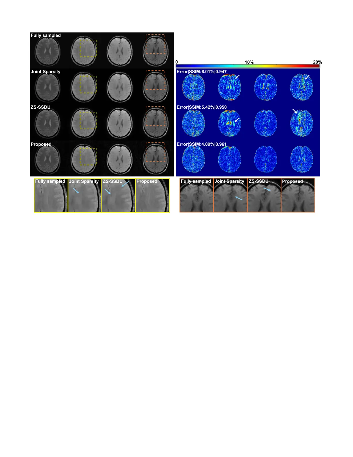
1 An Adaptiv e , Disentangled Representation f or Multidimensional MRI Reconstr uction Ruiyang Zhao and F an Lam Abstract — W e present a new appr oach f or representing and reconstructing multidimensional magnetic resonance imaging (MRI) data. Our method b uilds on a novel, learned feature-based image representation that disentangles dif- ferent types of features, such as g eometry and contrast, into distinct low-dimensional latent spaces, enabling bet- ter exploitation of feature correlations in multidimensional images and incorporation of pre-learned priors specific to different feature types for reconstruction. More specif- ically , the disentanglement was achieved via an encoder- decoder network and image transfer training using large public data, enhanced by a style-based decoder design. A latent diffusion model was introduced to impose str onger constraints on distinct feature spaces. New reconstruc- tion formulations and algorithms were developed to in- tegrate the learned representation with a zer o-shot self- supervised learning adaptation and subspace modeling. The proposed method has been evaluated on accelerated T 1 and T 2 parameter mapping, achieving improved perfor- mance over state-of-the-ar t reconstruction methods, with- out task-specific supervised training or fine-tuning. This work offers a new strategy for learning-based multidimen- sional image reconstruction where only limited data are av ailable f or problem-specific or task-specific training. Index T erms — Disentangled image representation, La- tent diffusion model, Multidimensional MR imaging, Self- supervised MRI reconstruction, Quantitative MRI. I . I N T R O D U C T I O N The success of deep learning has facilitated the paradigm shift in image reconstruction from generic “hand-crafted” reg- ularization/priors to learning and incorporating domain/task- specific priors via data-driven methods. In the realm of MRI, one mainstream approach is unrolling iterati ve optimization al- gorithms into cascaded deep neural networks that map directly from an initial reconstruction (or k -space measurements) to the reconstructed image. These networks are trained end-to-end in a supervised fashion when high-quality , fully-sampled images are av ailable [1]–[4], or in a self-supervised manner lev eraging only noisy or incomplete measurements [5]–[7]. While both training strategies ha ve demonstrated impressi ve performance, they typically require large quantities of training data to achiev e reliable results. Furthermore, the task-specific nature This work was suppor ted in par t by the f ollowing grants: NSF-CBET 1944249, NIH/NIGMS 5R35GM14296. R. Zhao is with the Depar tment of Electrical and Computer Engi- neering and Beckman Institute for Adv anced Science and T echnology , University of Illinois Urbana-Champaign. F . Lam is with the Depar tment of Bioengineering and Beckman Institute for Advanced Science and T echnology , University of Illinois Urbana-Champaign, IL 61801 USA (e-mail: fanlam1@illinois .edu). of these approaches renders the learned models vulnerable to variations in acquisition protocols, data quality , and domain shifts [8], [9]. An alternativ e learning-based image reconstruction ap- proach is to pre-learn a “prior” that can be flexibly incor- porated (or “plugged in”) into iterativ e algorithms considering task-specific forward models, rather than learning the inv erse mapping end-to-end. For example, prior learning techniques such as score-based diffusion models have been extensi vely in vestigated [10]–[12], along with various algorithms designed to integrate these learned priors [13]–[16]. These methods circumvent the need of retraining for each new reconstruction task and can be more robust to acquisition and domain v aria- tions. While promising, their application in multidimensional imaging remains largely unexplored due to the scarcity of training data and challenges in effecti vely leveraging feature correlations across multiple image dimensions. For example, in multidimensional MRI applications such as quantitative parameter mapping [17]–[19], MR spectroscopic imaging [20], [21], or dynamic imaging [22], [23], acquiring large and div erse datasets for learning the entire spatiotemporal prior is often prohibitive considering the resources needed. Even with adequate data, strategies to more effecti vely exploit multidimensional feature correlations are needed. Another approach that has attracted more attention recently is using network-based representation of unknown images for zero-shot learning-based reconstruction. In this approach, the target image is modeled as the output of a network, typically via a decoder architecture that maps a low-dimensional feature vector (latent) into images. Compared to other learning-based methods, it offers several advantages: (1) it substantially reduces the degrees of freedom by reformulating image re- construction as the recov ery of low-dimensional latents; (2) it enhances generalizability across tasks, since the netw ork learns image representations rather than direct inv erse mapping; (3) it offers flexibility in data-limited settings, as the representation can be implemented using untrained networks (e.g., deep image prior [24], [25]), pre-trained networks (e.g., generati ve adversarial networks [26] and latent diffusion models [27]), or pre-trained networks plus experiment/task-specific fine-tuning or adaptation [28], [29]; and (4) by describing images via a set of features rather than individual voxel values, it enables ne w ways to constrain multidimensional images that often exhibit correlated features. For example, in quantitative MRI (qMRI), image contrast changes with acquisition parameters while the underlying anatomy (geometry) remains unchanged. There- fore, network-based representation offers a potential solution 2 to the data scarcity and generalization challenges, particularly in multidimensional acquisition settings. In this work, we proposed a new network-based representa- tion for reconstructing multidimensional MR images. Specif- ically , we introduced a model and learning strategy that sep- arate different types of image features such as geometry and contrast into distinct low-dimensional latent spaces, reducing the degrees of freedom for multidimensional images and en- abling flexible constraints on individual features. Latent dif fu- sion models were employed to provide feature-lev el generativ e priors on the disentangled latents for constrained reconstruc- tion. T o mitigate potential mismatch between representations pre-trained using large public datasets and application-specific data, we developed a novel algorithm that combines pretrained representations with task-specific adaptation through zero-shot self-supervised learning. W e demonstrated ef fecti ve disentan- glement achieved for geometry and contrast features in multi- contrast images and ev aluated its utility in multidimensional MR applications such as accelerated T 1 and T 2 mapping. The remaining of the paper is organized as follo ws: Section II provides some background on feature-base image represen- tation and its use in image reconstruction. Section III describes the proposed problem formulation and algorithm in details. Section IV e valuates the proposed method in two application examples, accelerated T 1 and T 2 mapping. Section V and VI provide some technical discussion and conclude the paper . I I . B AC K G R O U N D A. Feature-based Representation and Reconstruction In feature-based representation, the image of interest X is described as: X = D θ ( z ) , with z denoting a set of latent variables (typically lower dimensional than X ) and D θ ( . ) a network parameterized by θ mapping the latent to image space. Compared to the earlier kernel-based representation [30], [31], these network-based models offer more flexibility and circumvent the need to choose a specific kernel. W ith this model, the reconstruction problem can be formulated as estimating z and/or the network parameters θ by solving: ˆ z , ˆ θ = arg min z , θ ∥ A ( D θ ( z )) − y ∥ 2 2 , (1) where A and y denote the forward model and measured data, respectiv ely . Since the reconstruction is constrained to lie within the range space of D θ ( · ) , this approach may introduce substantial modeling errors from several sources: mismatch between the training data for representation learning and test data, low-dimensionality of z , and limitations of optimization algorithms. This issue has been observed in methods based on pretrained GANs that update only the latent v ariables z [26]. While jointly updating both z and θ can mitigate this issue, it requires early stopping and/or other careful regularizations to prevent overfitting to noise and artifacts. T o reduce representation error while maintaining effec- tiv e constraints, we will introduce a second-stage refinement network combined with a zero-shot self-supervised learning strategy to update the network parameters and latent-diffusion- based constraints. In addition, the proposed network is adapted Fig. 1. A disentangled representation (using “geometry” and “contrast” features as examples): Once lear ned, geometry and contrast latents can be sampled from respectiv e distributions and combined to gener ate images with target geometry or contrast. from a style-based architecture [32], [33], which has demon- strated stronger image representation capability than earlier generations of GANs, particularly for high-resolution images. B. Multidimensional Image Representation A straightforward extension of feature-based image repre- sentation to multidimensional imaging is to assign separate latents and network parameters to each image, i.e., X 1 = D θ 1 ( z 1 ) , X 2 = D θ 2 ( z 2 ) , . . . , X N t = D θ N t ( z N t ) , (2) where { X 1 , X 2 , . . . , X N t } denote the images acquired at dif- ferent times or parameters. Howe ver , modeling each image in- dependently ignores their inherent correlations and introduces unnecessarily more unknowns. T o this end, a common strategy is to enforce shared network parameters across all images ( θ 1 = θ 2 = · · · = θ N t ) and explore correlations in latent space. For example, similarity constraints can be introduced on adjacent latents (e.g., z i ≈ z i +1 ) by assuming that images acquired at neighboring time points share similar features. Additionally , multi-resolution architectures like StyleGAN can be utilized to impose in variance on certain latent components across images [32]–[34]. Although helpful, these methods rely on generic similarity assumptions that do not capture the true relationships among the latents for multidimensional images. T o better model feature correlations in the latent space, we propose learning a disentangled representation that de- composes the latent space into semantically distinct com- ponents. Considering contrast and geometry variations as an example, images with dif ferent contrast weightings { X c 1 , X c 2 , . . . , X c N t } are acquired in many applications such as quantitative MRI. If contrast variations can be modeled separately from geometry in the latent space (see Fig. 1), each image can be modeled using a shared geometry latent z g and contrast-specific latents { z c 1 , z c 2 , . . . , z c N t } , which leads to: X c i = D θ ( z g , z c i ) for i = 1 , 2 , . . . , N t . This disentangled representation better e xploits feature correlations and enables explicit control over distinct image features. The ne xt section describes our detailed methodology . 3 Fig. 2. (a) The proposed representation lear ning strategy . Image transf er losses are used to train the disentangled representation. The decoder combines geometr y latents from X g i ,c i with contrast latents from X g j ,c j to generate a new image (see r ight), which can be inter- preted as contrast transf er for X g i ,c i or geometry transfer f or X g j ,c j . (b) The FiLM bloc k f or f eature combination. At resolution l , the encoder feature maps F l enc are transformed into z l c through global aver age pooling (GAP) and a fully connected (FC) la yer . The resulting z l c is then split into modulation parameters γ l c and β c l , which are applied to modulate the decoder feature maps F l dec at the same lev el. I I I . P RO P O S E D M E T H O D A. Lear ning A Disentangled Image Representation Our target is to learn a model that enables explicit control of different features in the target images. T o this end, we propose a two-step learning strategy . The first step in volv es training an autoencoder to enable feature disentanglement through image transfer and latents regularization, while the second step focuses on learning priors distributions for disentangled latents using diffusion models. In this paper , we inv estigate the disentanglement of contrast and geometry features, with a specific focus on reconstructing images with dif ferent contrast- weightings, while the approach can be generalized to other types of features. More specifically , we first represent multicontrast images using two distinct sets of latents, i.e., geometry and contrast. T wo separate image encoders, E g ( · ) and E c ( · ) , were emplo yed to extract geometry and contrast information, respectively . The resulting latents were then combined by a decoder D θ ( · ) for image synthesis (Fig. 2). The autoencoder training is based on image transfer , where the decoder combines a geometry latent from one image with a contrast latent from another to synthesize cross-composed images, minimizing an image transfer loss: L t =   X g i ,c j − D θ ( E g ( X g i ,c i ) , E c ( X g j ,c j ))   2 F , (3) where X g i ,c i and X g j ,c j denotes image pairs with geometry g i and g j and contrast c i and c j . The target X g i ,c j corresponds Fig. 3. Feature disentanglement achie ved: High-quality T 1 w (first) and T 2 w (last) images can be generated by sampling a geometr y latent z g 1 from our lear ned latent diffusion model and combining it with two different contrast latents z c T 1 and z c T 2 , using the trained decoder. Interpolation between z c T 1 and z c T 2 produced images with consistent geometry but varying contrasts (middle images). Combining a different geometry latent with z c T 1 produced the same T 1 contrast but with different anatomical f eatures (bottom). to an image sharing the same geometry as X g i ,c i and the same contrast as X g j ,c j . T o further promote disentanglement, we introduced a multi- resolution, StyleGAN-like architecture. The contrast encoder E c ( · ) produces latents at multiple resolutions, which are injected into the decoder via Feature-wise Linear Modulation (FiLM) [35]. For example, as shown in Fig. 2(b), the feature map F l enc extracted by E c ( · ) at a giv en resolution lev el l is transformed into scale and shift vectors γ l , β l ∈ R B × C l , where B denotes the batch size and C l the number of channels. The corresponding decoder features F l dec ∈ R B × C l × H l × W l are modulated as: FiLM  F l dec    γ l , β l  = γ l ⊙ F l dec + β l , (4) where ⊙ is element-wise multiplication, with γ l and β l broadcasted over the spatial dimensions ( H l , W l ) . This mech- anism encourages the model to represent contrast as global, layer-wise intensity transformations while preserving spatial structure in the decoder . By explicitly modulating feature at multiple resolutions, FiLM of fers an effecti ve way to control contrast-related variations without altering spatial content, thereby promoting geometry–contrast disentanglement. T o model the distributions of latents z g (geometry) and z c (contrast), we trained a latent diffusion model that learns “disentangled” generative priors for multicontrast images. The loss function for training the dif fusion model is defined as: L LDM g/c = E z g/c ,ϵ ∼N (0 , 1) ,t h   ϵ − ϵ θ g/c  z g /c , t    2 F i . (5) where t is the time step in dif fusion models, θ g and θ c denotes the parameters for the score functions of z g and z c , respectively . W e used a time-conditioned UNet as the backbone of ϵ θ g/c [36]. The model was trained using large- scale public datasets including HCP and Kirby21 datasets [37], [38]. 4 Algorithm 1 The Proposed Reconstruction Algorithm with the Learned Representation and Latent Diffusion Prior Require: Measurements d , Forward Operator A ( · ) , Decoder D θ ( · ) , Refinement Network N θ N ( · ) , Pretrained Noise Predictor ϵ θ g ( · ) , Diffusion Parameters ¯ α t d , η , δ , Hyperparameter γ , Data Consistency Update Steps C 1: Initialize { z g t ,T d } , { z c t } ∼ N (0 , I ) and refinement params θ N 2: for t d = T d − 1 , . . . , 0 do 3: Diffusion step : Predict noise { ˆ ϵ t,t d +1 } = ϵ θ g ( { z g t ,t d +1 } , t d + 1) 4: Estimate clean latent via T weedie’ s formula: { ¯ z g t , 0 } = 1 √ ¯ α t d +1  { z g t ,t d +1 } − √ 1 − ¯ α t d +1 { ˆ ϵ t,t d +1 }  5: Update via DDIM: { z ′ g t ,t d } = √ ¯ α t d { ¯ z g t , 0 } + p 1 − ¯ α t d − η δ 2 { ˆ ϵ t,t d +1 } + η δ { ϵ } , where ϵ ∼ N (0 , I ) 6: if t ∈ C (data consistency steps) then 7: Data consistency update: { ˆ z g t } , { ˆ z c t } , ˆ θ N = arg min { z g t } , { z c t } , θ N ∥ A Θ ( { D θ ( z g t , z c t ) } ) − d Θ ∥ 2 F | {z } measured part + ∥ A Λ ( N θ N ( { D θ ( z g t , z c t ) } , d Θ , A Θ )) − d Λ ∥ 2 F | {z } held-out part 8: Resample(blend DDIM and DC): { z g t ,t d } = StochasticResample ( { ˆ z g t } , { z ′ g t ,t d } , γ ) 9: else 10: { z g t ,t d } = { z ′ g t ,t d } 11: end if 12: end for 13: Final reconstruction : X = N ˆ θ N ( { D θ ( ˆ z g t , ˆ z c t ) } , d , A ) B. Reconstruction F or mulation and Algorithm Lev eraging the pre-trained representation D θ ( . ) , we propose the following multidimensional reconstruction formulation: { ˆ z g t } , { ˆ z c t } , ˆ θ N = arg min { z g t } , { z c t } , θ N ∥ A ( X ) − d ∥ 2 F + N t X t =1 λ g t R g ( z g t ) , s.t. X = N θ N ( { D θ ( z g t , z c t ) } ) . (6) The first term in Eq. (6) enforces data consistency . A is the encoding operator , X ∈ C N × N t is the unknown image with N vox els and N t ”time” points, and d represents the acquired data. The second term re gularizes the geometry latents z g t with R g , realized via a latent diffusion prior (see Section III.A). Although both geometry and contrast priors can be learned and applied, only the geometry latent diffusion prior was adopted, due to a distribution mismatch between the training and experimental data (see Section III-C). Finally , X is con- strained within the range space of the adapti ve representation N θ N ( { D θ ( z g t , z c t ) } ) , where a refinement network N θ N ( . ) further adapts decoder outputs { D θ ( z g t , z c t ) } (a set of images across ”time”) to the acquired data domain to reduce any representation bias. A zero-shot learning strategy is employed to estimate the parameters θ N using only the acquired data. This formulation enables effecti ve exploitation of redun- dancy in multidimensional images. F or image sequences with varying contrasts, the anatomy remains unchanged. W e can enforce shared geometry latents, e.g., z g 1 = z g 2 = · · · = z g N t , reducing the number of unknowns (see specific cases in Section IV). Moreover , the disentangled representation allows geometry priors learned from large public datasets with many subjects but limited contrasts to be transferred to specific applications which may ha ve richer contrast variations. T o solve Eq.(6), we adapted the algorithm from [27] to incorporate data consistency constraints during the rev erse latent diffusion steps that enforces pre-learned feature-lev el prior . The overall algorithm is summarized in Algorithm 1. More specifically , starting from Gaussian noise, the geometry latents { z g t ,t d +1 } (at diffusion step t d + 1 ) are progressively denoised via an unconditional re verse process of a Denoising Diffusion Implicit Model (DDIM) [39], where T weedie’ s for - mula provides an estimate of the clean latent { ¯ z g t , 0 } at each step. At selected re verse diffusion steps, a conditional update was applied to adjust { z g t } , { z c t } and θ N by minimizing the data consistency loss as follo ws: { ˆ z g t } , { ˆ z c t } , ˆ θ N = arg min { z g t } , { z c t } , θ N ∥ A ( N θ N ( { D θ ( z g t , z c t ) } )) − d ∥ 2 F , (7) which can be optimized using gradient descent. The updated geometry latents { ˆ z g t } are then stochastically resampled back to continue the reverse diffusion process. Finally , the decoder and refinement network are applied to { ˆ z g t } and { ˆ z c t } to produce the reconstructed image. Directly updating θ N may lead to overfitting due to the large number of parameters. Thus, we adopted the data partitioning strategy from the SSDU approach [5]. Data were partitioned into two disjoint subsets: d = d Θ ∪ d Λ (with matched forward operators A Θ and A Λ ), leading to the follo wing modified data consistency loss: { ˆ z g t } , { ˆ z c t } , ˆ θ N = arg min { z g t } , { z c t } , θ N ∥ A Θ ( { D θ ( z g t , z c t ) } ) − d Θ ∥ 2 F + ∥ A Λ ( N θ N ( { D θ ( z g t , z c t ) } , d Θ , A Θ )) − d Λ ∥ 2 F . (8) In this formulation, the first term enforces data consistency with respect to (w .r .t.) { z g t } and { z c t } using d Θ as the target. The second term corresponds to the SSDU reconstruction loss, where the refinement network takes both the decoder output { D θ ( z g t , z c t ) } and d Θ as input and uses the other partition d Λ as the target. The loss is minimized w .r .t. { z g t } , { z c t } , and θ N . This “joint” update of { z g t } , { z c t } , and 5 Fig. 4. Reconstructed images (top left panel) from experimental T 1 mapping data and the corresponding error maps (top right panel) at AF=6. Images acquired with diff erent flip angles are shown in diff erent columns while results from different methods in respectiv e ro ws. Zoomed-in regions from the images are shown in the bottom panel with ar tifacts that were reduced b y our method indicated by blue arrows . Mean-squared errors and SSIM values are sho wn in the the error maps. The proposed method achie ved the lowest error and highest SSIM, with most noise-lik e residuals. θ N is computationally more ef ficient than solving latent first followed by the SSDU-based adaptation. The first term can be viewed as a regularization on { z g t } and { z c t } for the SSDU loss, facilitating con ver gence with a small number of update steps. During each gradient descent step, different partitions were created as ’ data augmentation’ [40]. The refinement network N θ N ( · ) was implemented as an unrolled network adapted from [3]. Combining the proposed representation with the refinement network achieved better performance compared to SSDU-based reconstruction alone or reconstruction using only the learned representation (see Results). C . T raining and Other Implementation Details W e pre-trained our representation model using the HCP and Kirby21 datasets [37], [38]. T 1 -weighted (T 1 w) and T 2 - weighted (T 2 w) images from the HCP database, and T 1 w , FLAIR, T 1 mapping (flip angles = 15 ◦ and 60 ◦ ), and T 2 mapping (TE = 30 ms and 80 ms) data from the Kirby21 database were used. The proposed reconstruction method was ev aluated using in-house T 1 and T 2 mapping data, where data from one subject were used for hyperparameter tuning (validation) and data from two subjects were used for testing. Network training and reconstruction were performed on a Linux server with an NVIDIA A40 GPU and implemented in PyT orch 2.0.1. The Adam optimizer was used with a batch size of 64 for both the autoencoder and diffusion model training. Reconstruction methods based on joint sparsity and low-rank plus joint sparsity for comparison were implemented in MA TLAB R2020b. I V . E X P E R I M E N T S A N D R E S U L T S A. Effectiv e Feature Disentanglement W e first ev aluated the feature disentanglement of the pro- posed representation. As shown in Fig. 3, with the geometry latents of two images with the same anatomy fixed, inter- polating between their respectiv e contrast latents generated images with varying contrasts but identical anatomy , demon- strating effecti ve separation of geometric and contrast features. These results also support that images with dif ferent contrast weightings can be produced by combining a shared geometry latent with varying contrast latents, a strong constraint for multicontrast image reconstruction. This disentanglement property directly motiv ates the appli- cation of our learned representation to MR parameter mapping, where sequences of images with varying contrasts are recon- structed and quantified. In this w ork, we ev aluated the utility of the proposed representation and image reconstruction using quantitativ e T 1 and T 2 mapping tasks. 6 Fig. 5. T 1 mapping results at 6 × acceleration (AF=6; brain mask ed). The proposed method preserved spatial details better with the high- est mapping accuracy , as shown in the estimated T 1 maps (middle), zoomed-in regions (top), and the corresponding error maps (bottom). The ov erall errors and SSIM v alues for T 1 maps are shown. B. In Vivo Experiments All in vivo experiments were performed with local IRB approv al. T 1 mapping data were acquired using a v ariable flip angles (vF As) protocol with a spoiled gradient echo sequence on a 3T scanner equipped with a 20-channel head coil [41]. Acquisition parameters were: TR/TE = 40 / 12 ms , flip angles = 5 ◦ , 10 ◦ , 15 ◦ , 20 ◦ , 30 ◦ , 40 ◦ , field of view (FO V ) = 210 × 210 × 107 mm 3 , and matrix size = 192 × 192 × 32 . T 2 mapping data were acquired using a multi-slice multi- spin-echo sequence on a 3T scanner with a 20-channel head coil [42]. Parameters were: TR = 3110 ms , 15 echoes with TE 1 = 11 . 5 ms and echo spacing ∆TE = 11 . 5 ms . 8 slices were acquired, each with FO V = 220 × 200 mm 2 , matrix size = 224 × 192 , and slice thickness = 3 mm . For both types of acquisitions, fully sampled data were acquired and retrospectiv ely undersampled using a variable density random phase encoding mask (center fully sampled with Gaussian density decay tow ard the periphery) with dif- ferent acceleration factors (AFs). Coil sensitivity maps were estimated via ESPIRiT [43], using 18 central k -space lines from the first flip angle/TE. In the T 2 mapping experiment, 6 central k -space lines at all TEs were additionally acquired for subspace estimation [44]. For accelerated T 1 mapping, 6 central k -space lines were acquired at remaining flip angles, but no subspace estimation was performed because only six flip angles were a v ailable. C . T 1 mapping Results For T 1 mapping, we compared the proposed method with a joint sparsity constrained reconstruction [45] and a state-of- the-art zero-shot self-supervised reconstruction method (ZS- SSDU) [40]. W e selected ZS-SSDU as a primary base- line because our method also follows a zero-shot learning paradigm, requiring no supervised re-training or fine-tuning on domain-specific datasets. Representativ e reconstructed im- ages at AF=6 are shown in Fig. 4. The proposed method consistently produced reconstructions with improved quality Fig. 6. T 2 mapping results (first ro w) and error maps (second row) from diff erent methods at AF=8; The ov erall errors and SSIM for T 2 maps were also shown in the error maps (top left corners). As can be seen, lower reconstruction error and better preservation of details were observed f or the proposed method (last column). Zoomed-in regions fur ther illustrate the reduced errors achie ved. and reduced errors across different contrasts (F As) compared to other methods. The corresponding T 1 maps are shown in Fig. 5. The proposed method achie ved the most accurate T 1 estimates w .r .t. the fully sampled reference as shown by the lowest relati ve ℓ 2 errors and highest SSIM values, ef- fectiv ely suppressing artifacts. The zoomed-in re gions further demonstrate a better preservation of structural details by the proposed method. The ZS-SSDU method, although produced lower errors than the joint sparsity method, seemed to result in strong bias in certain localized areas (Fig. 5, last row). These results demonstrated that the proposed representation can work synergistically with zero-shot self-supervised learning, leading to improved reconstruction and quantification performance. More quantitativ e comparisons under dif ferent AFs are shown in Fig. 7. D . T 2 mapping Results For T 2 mapping, the proposed method was further combined with low-rank/subspace modeling [46]. Specifically , the under- lying image X ∈ C N × N t can be modeled as: X = U ˆ V , where U ∈ C N × r represents the spatial coefficients, ˆ V ∈ C r × N t a set of temporal basis, and r the subspace order/rank. ˆ V can be pre-determined from central k -space data. This introduced a complementary constraint to the learned representation. As a result, the loss function in Eq. (8) is changed into: { ˆ z g t } , { ˆ z c t } , ˆ θ N = arg min { z g t } , { z c t } , θ N ∥ A Θ ( { D θ ( z g t , z c t ) } ˆ V H ˆ V ) − d Θ ∥ 2 F + ∥ A Λ ( N θ N ( { D θ ( z g t , z c t ) } ˆ V H , d Θ , A Θ , ˆ V ) ˆ V ) − d Λ ∥ 2 F . (9) In the first term, the representation is projected onto the sub- space (assuming orthonormal temporal basis). In the second term, instead of adapting all images directly , we perform refinement only on the spatial coefficients, which reduces the 7 Fig. 7. P arameter mapping errors at diff erent AFs f or the T 1 (left) and T 2 (right) mapping data. The proposed method consistently achieved the lowest errors across all AFs, with more pronounced improvements at higher AFs. Error bars denote standard deviation of errors across all subjects and slices. number of trainable parameters in the refinement network and improv es the efficienc y of zero-shot learning [47]. The refinement network takes both the spatial coef ficients estimate { D θ ( z g t , z c t ) } ˆ V H and the temporal basis ˆ V as input (for the data consistency block during unrolling). The output are refined spatial coefficients, which are then recombined with ˆ V as: N θ N ( { D θ ( z g t , z c t ) } ˆ V H , d Θ , A Θ , ˆ V ) ˆ V to generate the full set of reconstructed images. Fig. 6 compares T 2 mapping results estimated from recon- structions produced by different methods at AF = 8. The over - all estimation errors and SSIM v alues w .r .t. the fully sampled data were computed within the brain regions with T 2 values lower than 500 ms. The proposed method integrating our disentangled representation and subspace modeling yielded superior performance over a subspace reconstruction method with joint sparsity regularization [44] and the ZS-SSDU method. These results also demonstrated the flexibility of the proposed representation to be combined with complementary constraints. Fig. 7 further demonstrates lower reconstruction errors consistently achiev ed by the proposed method across different AFs. V . D I S C U S S I O N W e presented an adaptiv e, feature-disentangled represen- tation for multidimensional MRI reconstruction. A unique feature of our approach is its ability to more explicitly exploit feature correlations through disentanglement, where geometry and contrast variations are captured by distinct latent spaces. This design substantially reduces the degrees of freedom while enabling flexible and semantically meaningful constraints. An- other key component is the second-stage refinement network, which adapts the pretrained representation to application- specific domains. By employing a zero-shot self-supervised learning strategy , the proposed refinement effecti vely circum- vents the overfitting issue often observed in methods that jointly update both latent variables and network parameters. One important design choice is whether geometry latents should be shared across all images with different contrasts. T o ev aluate this, we conducted abalation studies using T 1 mapping data, first comparing reconstructions using a single shared geometry latent across all F As versus F A-dependent ge- ometry latents. Fig. 8 sho ws that enforcing a shared geometry latent across all F As produced better reconstruction in terms Fig. 8. An ablation study using the T 1 mapping data (AF = 8 ); Map- ping errors (mean ± standard deviation) summarized across different subjects and slices are shown in the reconstructed T 1 maps. Recon- structions without the refinement network exhibit substantially higher errors. Compared to using independent latents, the proposed method with shared geometry latents yielded slightly lo wer reconstruction errors and variability . Error maps fur ther highlight stronger ar tifacts when the shared latent constraint is not enf orced. of quantitativ e T 1 maps, indicating the benefit of degrees- of-freedom reduction leveraging shared geometry features. Another ablation study shows that removing the refinement network deteriorated the results substantially (Without refine- ment network case in Fig. 8), supporting its role in reducing representation errors and domain shifts. These results demon- strate the importance of adapting pretrained representations to application-specific domains, particularly when only limited or mismatched training data are a vailable. An important question that may be raised is whether ge- ometry and contrast can be fundamentally disentangled. In practice, the definition of these two, especially for “contrast”, is not absolute. In our formulation, the “geometry” latent essentially captures structural features shared across multiple MR contrasts, while the “contrast” latent represents image- specific v ariations driv en by acquisition parameters or relax- ation effects. While the proposed disentanglement is learned in a data-driven manner within the MRI domain, it may be extended to more general multimodal settings (e.g., MRI and CT). Howe ver , this would require rethinking how geometry and contrast are defined, as the underlying imaging physics and signal characteristics differ substantially . Achieving modality in variant geometry representations may require training on co-registered multimodal data and the design of specialized training strategies. Sev eral recent studies have explored the disentanglement concepts for multimodal tasks such as joint MRI-CT image analysis and segmentation [48], [49]. These methods typically aim to separate modality in variant fea- tures from modality specific appearance to facilitate down stream tasks. Extending such approaches to image recon- struction, howe ver , would require more effecti ve utilization of multimodal feature correlations and careful consideration of representation accuracy . Multimodal reconstruction using disentangled representations remains an open and promising direction for future research. W e adopted the StochasticResample strategy proposed in 8 [27] in our algorithm (Algorithm 1), to map the data consis- tency update output ˆ z g t back to the diffusion sampling trajec- tory z g t ,t d . Compared to directly adding noise to the latents (e.g., applying the forward diffusion process), this strategy can reduce variance and lead to less noisy reconstruction [27]. Mathematically , the StochasticResample can be expressed as sampling from the follo wing distribution: p ( z g t ,t d | ˆ z g t , z ′ g t ,t d ) = N σ 2 t √ ¯ α t ˆ z g t + (1 − ¯ α t ) z ′ g t ,t d σ 2 t + (1 − ¯ α t ) , σ 2 t (1 − ¯ α t ) σ 2 t + (1 − ¯ α t ) I ! , (10) where the mean can be viewed as the a weighted combina- tion of data consistency update output ˆ z g t and the uncon- ditional DDIM latent sample z ′ g t ,t d . σ 2 t is defined as σ 2 t = γ  1 − ¯ α t − 1 ¯ α t   1 − ¯ α t ¯ α t − 1  . In this framew ork, γ controls the tradeoff between prior consistency and data consistency . For example, if γ → 0 , z g t ,t d will reduce to z ′ g t ,t d , which result in unconditional DDIM sampling and poor data consistency . In practice, we found a relatively lar ge range of γ can result in similar reconstruction results. W e set γ = 35 , which worked robustly across dif ferent cases in vestigated here. Another issue is reconstruction time. For the reverse pro- cess of diffusion model, we employed 500 DDIM steps and performed data consistency update ev ery 20 steps. Each data consistency update in volves 30 iterations of gradient descent to optimize { z g t } , { z c t } , θ N . Under these settings, the reconstruction requires approximately 15 minutes for T 1 mapping and 25 minutes for T 2 mapping. While the proposed representation provides a strong initialization that reduces the number of steps needed for self-supervised training, and the integration with subspace modeling further decreases the number of trainable parameters, updating the parameters for N θ N ( · ) remains computationally expensi ve. Future work may address this issue by pre-training the refinement network on a small quantity of in-domain data, thereby reducing the number of online adaptation steps required. In this work, disentanglement was enforced through an im- age transfer strategy . Future research may explore approaches that enforce disentanglement more explicitly in the latent space. For example, contrastiv e learning techniques could be employed to promote latent similarity across shared features and improve separation between geometry and contrast fea- tures [50], [51]. Alternativ e generativ e priors can be explored. For instance, models based on flow matching may accel- erate the sampling process, thus accelerating reconstruction [52]. Beyond MR parameter mapping, our method could be extended to other multidimensional MRI applications. In quantitativ e cardiov ascular imaging, for example, modeling motion and contrast variation is essential [53] and may require specialized network architectures with tailored feature disen- tanglement strategies. For applications inv olving inherently noisy data, such as low-field MRI or spectroscopic imaging, self-supervised denoising strategies could be integrated with autoencoder training and refinement network updates to en- hance SNR. V I . C O N C L U S I O N This work presented a nov el approach for multidimen- sional MRI reconstruction that lev erages adaptiv e, feature- based disentangled representations. The learned disentangled representation effecti vely exploits shared and distinct image features in multidimensional data, where the associated feature priors can be pre-trained on large public data and adapted to specific applications. Our reconstruction method uses a zero-shot, self-supervised fine-tuning strate gy , eliminating the need for extensi ve task-specific training data while maintaining strong generalization across acquisition settings. Experimental results from accelerated T 1 and T 2 mapping demonstrated the effecti veness of our proposed method. Our approach offers a promising direction for learning-based multidimensional image reconstruction with limited data for task/application- specific supervised training. R E F E R E N C E S [1] K. Hammernik et al. , “Learning a variational network for reconstruction of accelerated mri data, ” Magn. Reson. Med. , vol. 79, pp. 3055–3071, 2018. [2] J. Sun et al. , “Deep ADMM-Net for compressive sensing MRI, ” Proc. NeurIPS , vol. 29, 2016. [3] H. K. Aggarw al et al. , “MoDL: Model-based deep learning architecture for inv erse problems, ” IEEE Tr ans. Med. Imag. , vol. 38, pp. 394–405, 2019. [4] V . Monga et al. , “ Algorithm unrolling: Interpretable, efficient deep learning for signal and image processing, ” IEEE Signa. Pr oc. Mag. , vol. 38, pp. 18–44, 2021. [5] B. Y aman et al. , “Self-supervised learning of physics-guided recon- struction neural networks without fully sampled reference data, ” Magn. Reson. Med. , vol. 84, pp. 3172–3191, 2020. [6] M. Akcakaya et al. , “Unsupervised deep learning methods for biological image reconstruction and enhancement: An overvie w from a signal processing perspective, ” IEEE Signa. Pr oc. Mag . , vol. 39, pp. 28–44, 2022. [7] C. Millard and M. Chiew , “ A theoretical framework for self-supervised MR image reconstruction using sub-sampling via variable density Nois- ier2Noise, ” IEEE T rans. Comput. Imag. , vol. 9, pp. 707–720, 2023. [8] M. Z. Darestani et al. , “Measuring robustness in deep learning based compressiv e sensing, ” in Proc. ICML , 2021, pp. 2433–2444. [9] R. Heckel et al. , “Deep learning for accelerated and robust MRI reconstruction, ” Magn. Reson. Mater . Phys. Biol. Med. , vol. 37, pp. 335– 368, 2024. [10] P . V incent, “ A connection between score matching and denoising au- toencoders, ” Neural Comput. , vol. 23, pp. 1661–1674, 2011. [11] J. Ho et al. , “Denoising diffusion probabilistic models, ” in Proc. NeurIPS , vol. 33, 2020, pp. 6840–6851. [12] Y . Song and S. Ermon, “Generative modeling by estimating gradients of the data distribution, ” in Pr oc. NeurIPS , vol. 32, 2019, p. 6392. [13] A. G ¨ ung ¨ or et al. , “ Adaptive diffusion priors for accelerated MRI reconstruction, ” Med. Imag. Anal. , vol. 88, p. 102872, 2023. [14] U. S. Kamilov et al. , “Plug-and-play methods for integrating physical and learned models in computational imaging: Theory , algorithms, and applications, ” IEEE Signal Proc. Mag . , vol. 40, pp. 85–97, 2023. [15] H. Chung et al. , “Diffusion posterior sampling for general noisy in verse problems, ” in Pr oc. ICLR , 2023. [16] G. W ebber and A. J. Reader , “Diffusion models for medical image reconstruction, ” BJR— Artificial Intelligence , vol. 1, p. ubae013, 2024. [17] D. Ma et al. , “Magnetic resonance fingerprinting, ” Natur e , vol. 495, pp. 187–192, 2013. [18] S. Ma et al. , “Three-dimensional simultaneous brain T 1 , T 2 , and ADC mapping with MR multitasking, ” Magn. Reson. Med. , vol. 84, pp. 72–88, 2020. [19] Z. Meng et al. , “ Accelerating T 2 mapping of the brain by integrating deep learning priors with lo w-rank and sparse modeling, ” Magn. Reson. Med. , vol. 85, pp. 1455–1467, 2021. [20] S. Posse et al. , “MR spectroscopic imaging: principles and recent advances, ” J. Magn. Reson. Imag. , vol. 37, pp. 1301–1325, 2013. 9 [21] F . Lam et al. , “High-Dimensional MR spatiospectral imaging by in- tegrating physics-based modeling and data-driven machine learning: current progress and future directions, ” IEEE Signal Proc. Mag . , vol. 40, pp. 101–115, 2023. [22] J. A. Oscanoa et al. , “Deep learning-based reconstruction for cardiac MRI: a revie w , ” Bioengineering , vol. 10, p. 334, 2023. [23] A. G. Christodoulou and S. G. Lingala, “ Accelerated dynamic magnetic resonance imaging using learned representations: A new frontier in biomedical imaging, ” IEEE Signal Proc. Mag . , vol. 37, pp. 83–93, 2020. [24] D. Ulyanov et al. , “Deep image prior , ” in Pr oc. IEEE CVPR , 2018, pp. 9446–9454. [25] J. Y oo et al. , “Time-dependent deep image prior for dynamic MRI, ” IEEE T rans. Med. Imag. , vol. 40, pp. 3337–3348, 2021. [26] A. Bora et al. , “Compressed sensing using generative models, ” in Pr oc. ICML , 2017, pp. 537–546. [27] B. Song et al. , “Solving inv erse problems with latent diffusion models via hard data consistency , ” in Proc. ICLR , 2024. [28] S. A. Hussein et al. , “Image-adaptive GAN based reconstruction, ” in Pr oc. AAAI Conf. Artif. Intell. , vol. 34, no. 04, 2020, pp. 3121–3129. [29] D. Narnhofer et al. , “In verse GANs for accelerated MRI reconstruction, ” in W avelets and Sparsity XVIII , vol. 11138, 2019, pp. 381–392. [30] G. W ang and J. Qi, “PET image reconstruction using kernel method, ” IEEE T rans. Med. Imag. , vol. 34, pp. 61–71, 2014. [31] Y . Li et al. , “Constrained MRSI reconstruction using water side infor- mation with a kernel-based method, ” in Pr oc. Int. Soc. Magn. Reson. Med. , 2018, p. 0166. [32] T . Karras et al. , “ A style-based generator architecture for generativ e adversarial networks, ” in Proc. IEEE CVPR , 2019, pp. 4401–4410. [33] T . Karras et al. , “ Analyzing and improving the image quality of stylegan, ” in Proc. IEEE CVPR , 2020, pp. 8110–8119. [34] V . A. K elkar and M. Anastasio, “Prior image-constrained reconstruction using style-based generativ e models, ” in Proc. ICML , 2021, pp. 5367– 5377. [35] E. Perez et al. , “Film: V isual reasoning with a general conditioning layer , ” in Pr oc. AAAI Conf. Artif. Intell. , vol. 32, no. 1, 2018. [36] R. Rombach et al. , “High-resolution image synthesis with latent diffu- sion models, ” in Proc. CVPR , 2022, pp. 10 684–10 695. [37] D. C. V an Essen et al. , “The WU-Minn human connectome project: an overvie w , ” Neuroima ge , vol. 80, pp. 62–79, 2013. [38] B. A. Landman et al. , “Multi-parametric neuroimaging reproducibility: a 3-T resource study , ” Neur oimage , vol. 54, pp. 2854–2866, 2011. [39] J. Song et al. , “Denoising dif fusion implicit models, ” in Pr oc. ICLR , 2021. [40] B. Y aman et al. , “Zero-shot self-supervised learning for MRI reconstruc- tion, ” in Pr oc. ICLR , 2022. [41] W . Bian et al. , “Improving quantitative MRI using self-supervised deep learning with model reinforcement: demonstration for rapid T 1 mapping, ” Magn. Reson. Med. , vol. 92, pp. 98–111, 2024. [42] X. Peng et al. , “ Accelerated exponential parameterization of T 2 re- laxation with model-driven low rank and sparsity priors (MORASA), ” Magn. Reson. Med. , vol. 76, pp. 1865–1878, 2016. [43] M. Uecker et al. , “ESPIRiT—an eigenv alue approach to autocalibrating parallel MRI: where SENSE meets GRAPP A, ” Magn. Reson. Med. , vol. 71, pp. 990–1001, 2014. [44] B. Zhao et al. , “ Accelerated MR parameter mapping with low-rank and sparsity constraints, ” Magn. Reson. Med. , vol. 74, pp. 489–498, 2015. [45] A. Majumdar and R. K. W ard, “ Accelerating multi-echo T 2 weighted MR imaging: analysis prior group-sparse optimization, ” J. Magn. Reson , vol. 210, pp. 90–97, 2011. [46] Z.-P . Liang, “Spatiotemporal imaging with partially separable functions, ” in Proc. IEEE Int. Symp. Biomed. Imag. , 2007, pp. 988–991. [47] M. Zhang et al. , “Zero-shot self-supervised joint temporal image and sensitivity map reconstruction via linear latent space, ” in Proc. MIDL , 2024, pp. 1713–1725. [48] A. Chartsias et al. , “Disentangled representation learning in cardiac image analysis, ” Med. Imag. Anal. , vol. 58, p. 101535, 2019. [49] J. Jiang and H. V eeraraghavan, “Unified cross-modality feature disentan- gler for unsupervised multi-domain MRI abdomen organs se gmentation, ” in Proc. MICCAI , 2020, pp. 347–358. [50] A. Radford et al. , “Learning transferable visual models from natural language supervision, ” in Proc. ICML , 2021, pp. 8748–8763. [51] J. Ouyang et al. , “Representation disentanglement for multi-modal brain MRI analysis, ” in Proc. IPMI , 2021, pp. 321–333. [52] Y . Lipman et al. , “Flo w matching for generative modeling, ” in Proc. ICLR , 2023. [53] A. G. Christodoulou et al. , “Magnetic resonance multitasking for motion-resolved quantitative cardiovascular imaging, ” Natur e Biomed. Eng. , vol. 2, pp. 215–226, 2018.