A multimodal Transformer for InSAR-based ground deformation forecasting with cross-site generalization across Europe

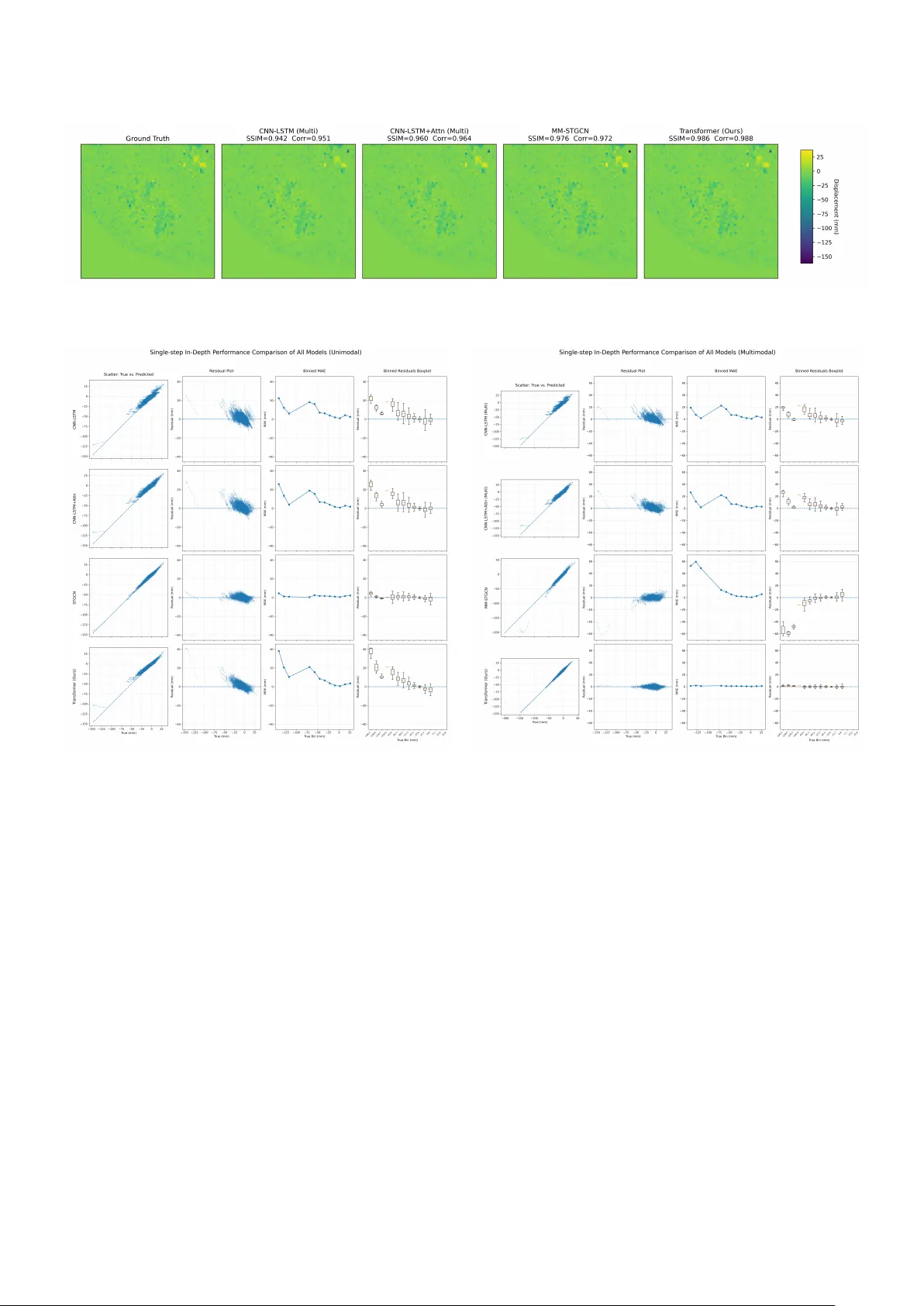
A multimodal T ransformer for InSAR-based ground deformation forecasting with cross-site generalization across Europe W endong Y ao a,b , Binhua Huang a,b , Soumyabrata Dev a,b, ∗ a The AD APT SFI Research Centr e, Dublin, Ir eland b School of Computer Science, Univer sity College Dublin, Belﬁeld, Dublin, Ir eland Abstract Near-real-time regional-scale monitoring of ground deformation is increasingly required to support urban planning, critical infras- tructure management, and natural hazard mitigation. While Interferometric Synthetic Aperture Radar (InSAR) and continental-scale services such as the European Ground Motion Service (EGMS) provide dense observ ations of past motion, predicting the next ob- servation remains challenging due to the superposition of long-term trends, seasonal cycles, and occasional abrupt discontinuities (e.g., co-seismic steps), together with strong spatial heterogeneity . In this study we propose a multimodal patch-based T ransformer for single-step, ﬁxed-interv al next-epoch no wcasting of dis- placement maps from EGMS time series (resampled to a 64 × 64 grid over 100 km × 100 km tiles). The model ingests recent displacement snapshots together with (i) static kinematic indicators (mean velocity , acceleration, seasonal amplitude) computed in a leakage-safe manner from the training windo w only , and (ii) harmonic day-of-year encodings. On the eastern Ireland tile (E32N34), the STGCN is strongest in the displacement-only setting, whereas the multimodal Transformer clearly outperforms CNN–LSTM, CNN–LSTM + Attn, and multimodal STGCN when all models recei ve the same multimodal inputs, achieving RMSE = 0.90 mm and R² = 0.97 on the test set with the best threshold accuracies. W e further assess transferability by training a single model on E32N34 and applying it, without ﬁne-tuning, to ﬁ ve unseen Euro- pean tiles spanning continuous subsidence, periodic motion, and co-seismic deformation. Across all six tiles the model maintains R 2 ≥ 0.93, with RMSE ranging from 0.7 to 3.2 mm and 71–87% of pixels within 1 mm. For co-seismic tiles, the high ov erall accuracy reﬂects robustness to strong time-series discontinuities and rapid post-event re-alignment once the step is present in the input history , rather than anticipation of earthquake occurrence. These results indicate that multimodal T ransformers can serve as accurate local nowcasters and transferable priors for EGMS-based deformation monitoring with limited local training data. K eywor ds: Interferometric Synthetic Aperture Radar (InSAR), Land subsidence Prediction, Multimodal deep learning, Cross-site generalisation 1. Introduction Ground deformation driv en by groundwater extraction, un- derground construction, hydrocarbon production and tectonic processes poses a persistent threat to buildings, transportation networks and critical infrastructure worldwide [1, 2, 3, 4]. In- terferometric Synthetic Aperture Radar (InSAR) has become a key technology for mapping such deformation with millimetre accuracy over large areas [5, 6, 7], and continental-scale ser- vices such as the European Ground Motion Service (EGMS) now deli ver harmonised ground-motion products across Europe [8, 9]. Ho wever , these products are intrinsically retrospecti ve: they describe ho w the ground has moved so far , but not how it is likely to mov e at the next acquisitions. In many opera- tional settings, ev en short-term information at the cadence of new satellite passes (on the order of a few days for Sentinel- ∗ Corresponding author . T el.: + 353 1896 1797. Email addr esses: wendong.yao@ucdconnect.ie (W endong Y ao), binhua.huang@ucdconnect.ie (Binhua Huang), soumyabrata.dev@ucd.ie (Soumyabrata Dev) 1 ov er Europe) can help operators track the ev olution of de- formation signals and prioritise sites for further inv estigation, complementing more traditional geodetic and engineering as- sessments rather than replacing them. W ithin Europe, these capabilities hav e recently been consoli- dated in the European Ground Motion Service (EGMS), an op- erational Copernicus Land Monitoring Service product based on Sentinel-1 SAR data [8, 9]. EGMS deli vers homogenised, quality-controlled ground motion information over the Euro- pean continent, including line-of-sight displacement time series and summary statistics such as mean velocity , linear accelera- tion and seasonal-motion parameters on a regular grid. This open and systematic service removes the need for bespoke In- SAR processing for many applications and o ﬀ ers, for the ﬁrst time, continental-scale time series of ground motion suitable for statistical analysis and machine-learning modelling [10]. Most current uses of EGMS and other InSAR products re- main retrospectiv e: they focus on mapping and attribution of observed deformation, for example by identifying subsiding ur- ban districts, unstable slopes or regions of aquifer compaction [11, 12]. Only a limited number of studies have attempted to for ecast future ground motion using data-driv en models, de- spite the potential value of short-term predictive capability for monitoring and maintenance workﬂo ws [13]. Recent work has begun to explore deep learning approaches for InSAR time se- ries, for instance using con volutional and recurrent neural net- works to detect deformation patterns or to model local displace- ment histories at speciﬁc sites [13]. Howe ver , these applications are typically restricted to one or a few locations, treat each pixel independently , or rely on relativ ely simple network architec- tures. Spatio-temporal deep learning models designed for struc- tured data provide a natural way to e xploit both the temporal dy- namics and spatial correlation of InSAR ground-motion ﬁelds. Spatio-temporal graph con volutional netw orks (STGCNs) [14], originally developed for tra ﬃ c forecasting, combine temporal con volutions with graph conv olutions deﬁned on a ﬁxed adja- cency structure and have pro ven e ﬀ ective for learning complex propagation patterns in networked systems. Self-attention and T ransformer architectures, ﬁrst proposed for natural language processing, have subsequently been adapted for time-series forecasting and for modelling spatial–temporal processes, al- lowing models to learn long-range and non-local dependencies without an explicit graph. At the same time, most existing forecasting studies in ground deformation still adopt a uni-modal perspecti ve, using only the displacement time series as input [13]. In contrast, operational products such as EGMS expose a richer set of information [9]: in addition to per-epoch displacement, each grid cell is associated with static motion descriptors (e.g. mean velocity , linear acceleration, seasonal amplitude) summarising its long- term behaviour , and the acquisition dates themselves encode clear seasonal cycles. Incorporating this multi-modal informa- tion into spatio-temporal deep learning models has the poten- tial to improv e forecasting skill, but this opportunity has not yet been systematically explored. In our previous work we proposed a con volutional neu- ral network–long short-term memory (CNN–LSTM) architec- ture for short-term InSAR ground deformation forecasting over eastern Ireland, using only sequences of displacement maps as input [15]. While this uni-modal approach achieved promis- ing skill, particularly when combined with an STGCN baseline on the same grid, its accuracy remained limited in regions with strong seasonal variability or low signal-to-noise ratio, and it did not explicitly exploit the static descriptors already a vailable from the EGMS processing chain. Also, this manuscript is related to our earlier study on EGMS / InSAR deformation forecasting [16], which inv esti- gated window-based forecasting models that are primarily trained and ev aluated in a site-speciﬁc manner . In contrast, the focus here is on transfer able single-step forecasting: we intro- duce a multimodal formulation that lev erages EGMS-deriv ed static deformation indicators and harmonic time encodings, and we de velop a patch-based Transformer that is e valuated under cross-site regimes, including zero-shot transfer across multiple European tiles. Accordingly , the model design choices, experi- mental protocols (cross-site and leakage-safe feature construc- tion), and conclusions di ﬀ er from [16]. The present study addresses these gaps by moving from a uni-modal to a multi-modal representation of EGMS ground motion and by systematically e valuating both graph-based and attention-based spatio-temporal deep learning architectures. W e construct a uniﬁed grid-based data set for a 100 km × 100 km EGMS tile covering eastern Ireland, in which each sample con- sists of: (i) a sequence of displacement maps; (ii) three static ground-motion indicator maps deri ved from the EGMS Le vel 3 product (mean velocity , acceleration and seasonal amplitude); and (iii) sinusoidal encodings of the acquisition day-of-year . On this multi-modal input we train and compare four archi- tectures: a con volutional–recurrent CNN–LSTM, its attention- augmented variant, a multi-modal STGCN and a newly de- signed spatio-temporal Transformer that operates on multi- channel image patches with global self-attention and residual next-step prediction. In this work we focus on single-step , ﬁxed-interval forecast- ing at the nativ e EGMS / Sentinel-1 cadence, i.e. predicting the displacement map at the next av ailable acquisition gi ven a his- tory of past observations and auxiliary variables. Such next- epoch forecasts are best viewed as a form of deformation now- casting and short-term trend projection, intended to support routine monitoring, screening and infrastructure management rather than stand-alone, long-horizon early-warning systems. Our main contributions are threefold: • W e construct a multimodal learning framew ork that com- bines recent displacement maps with static auxiliary lay- ers and temporal encodings, enabling the model to jointly exploit spatial susceptibility , seasonal forcing and local deformation history . W e show that this multimodal de- sign substantially improves single-step prediction accu- racy o ver using displacement maps alone. • W e design a dedicated Transformer architecture tailored to InSAR-based deformation forecasting and benchmark it against con volutional sequence models (CNN–LSTM, CNN–LSTM with attention) and a state-of-the-art spatio- temporal graph conv olutional netw ork (STGCN). On a tile in eastern Ireland, the proposed multimodal T ransformer achiev es the best overall single-step performance across RMSE, MAE, R 2 and multiple error-threshold accuracies. • Beyond local experiments, we systematically e valuate the spatial transferability of the multimodal Transformer . A model trained only on a single EGMS tile (E32N34) gen- eralises well to ﬁve additional tiles representing continu- ous subsidence, periodic motion, co-seismic displacement and quasi-stable conditions, maintaining R 2 ≥ 0 . 93 and high sub-millimetre accuracy . This demonstrates the po- tential of Transformer -based models as transferable priors for large-scale, EGMS-driv en deformation nowcasting in regions with limited local training data. 2 2. Data and study areas 2.1. Eur opean Gr ound Motion Service data Our analysis is based on the Level 3 (L3) products of the Eu- ropean Ground Motion Service (EGMS), part of the Copernicus Land Monitoring Service. EGMS provides harmonized ground- motion information ov er the European continent deri ved from multi-temporal interferometric processing of Sentinel-1 SAR images [8, 9]. The L3 product is a regularly gridded data set in which each grid cell aggregates one or more persistent or dis- tributed scatterers and stores a displacement time series along with sev eral summary statistics and quality indicators. For each grid cell, the L3 Up component used in this study contains: • the time series of vertical displacement with respect to a reference epoch; • the mean velocity estimated from a linear trend ﬁt to the time series; • a linear acceleration term capturing long-term curvature; • parameters describing the amplitude and phase of annual seasonal motion, deriv ed from harmonic regression; and • various uncertainty and quality metrics, including the stan- dard deviation of residuals. The underlying Sentinel-1 constellation provides a revisit time of 6 days over Europe in the ascending and descending orbits, enabling dense temporal sampling of ground motion at a nominal spatial resolution of approximately 20–30 m. The EGMS processing chain applies consistent orbit corrections, atmospheric delay mitigation, geocoding and rigorous quality control, producing a homogeneous long-term record of surface deformation suitable for regional and continental-scale appli- cations. In this work we exploit this consistency to study both local forecasting skill and cross-site generalization of our multi- modal T ransformer across di ﬀ erent deformation regimes in Eu- rope. For each 100 km × 100 km tile, the L3 Up prod- uct is deliv ered as a comma-separated values (CSV) ﬁle named EGMS_L3_EXXNYY_100km_U_2018_2022_1.csv , where EXXNYY encodes the tile identiﬁer in the EGMS tiling grid. The ﬁle contains all grid cells in the tile, with columns storing the geographic coordinates, ground-motion summary statistics and a series of displacement v alues for each Sentinel- 1 acquisition between 2018 and 2022. W e focus on this recent 5-year period to align with the operational EGMS version and to a void potential artefacts associated with the transition from the Sentinel-1A-only to the Sentinel-1A / B constellation. 2.2. Study ar eas and deformation re gimes T o ev aluate both local performance and cross-site generaliza- tion, we select six EGMS tiles distributed across Europe, cho- sen to represent a broad spectrum of ground-motion behaviours. T iles are identiﬁed using the standard EGMS naming con ven- tion, EXXNYY , where: • XX denotes the easting coordinate (in 100 km units, EPSG:3035) of the south-west corner of the tile’ s lower - left pixel; and • YY denotes the corresponding northing coordinate. The six tiles are grouped into three categories according to their dominant deformation regime: • Continuous and periodic def ormation: T iles E32N34 and E32N35 are located on the east coast of Ireland and encompass the greater Dublin region and surrounding low- lying coastal plain. Pre vious work has sho wn that these tiles exhibit a rich mixture of slow subsidence bowls, lo- calized uplift and pronounced seasonal signals related to hydrogeological forcing and anthropogenic loading. T ile E32N34 serves as our primary sour ce tile for training the multimodal Transformer , while both E32N34 and E32N35 are used to assess forecasting skill in regions dominated by gradual, often quasi-periodic deformation. • Long-term subsidence: T iles E39N30 and E44N23 pro- vide examples of more monotonic, long-term subsidence. These tiles cover urban and industrial areas underlain by compressible sediments and engineering structures where subsidence is driven by natural consolidation, groundwa- ter extraction and surface loading. The y are used to test whether a model trained on mixed-periodic beha viour can extrapolate persistent downw ard trends in previously un- seen settings. • Abrupt co-seismic displacement: T iles E48N24 and E58N17 encompass regions that experienced strong co-seismic deformation during recent moderate-to-lar ge earthquakes. These data are characterized by sharp spa- tial gradients and step-like temporal o ﬀ sets superimposed on otherwise relativ ely stable background motion. They constitute the most challenging scenario for cross-site gen- eralization, probing the ability of the model to reproduce sudden structural breaks in the time series. Across all tiles, the EGMS L3 product provides a dense sam- pling of ground motion over b uilt-up areas, transport corridors, exposed rock and other coherent scatterers. As is typical for C-band SAR, coverage is sparser in ve getated and agricultural zones, but the gridded product retains su ﬃ cient density to en- able interpolation to a regular raster representation suitable for con volutional and T ransformer-based neural networks. 2.3. Pr e-pr ocessing and feature construction T o build a common input representation for all models and tiles, we con vert the irregular grid of EGMS L3 points into a stack of raster maps at a spatial resolution of 64 × 64 pixels co v- ering the full 100 km × 100 km extent of each tile. For ev ery acquisition epoch, the vertical displacement values are interpo- lated onto this grid using linear scattered-data interpolation in the projected (easting, northing) coordinate system, yielding a displacement cube of size T × H × W per tile. 3 W e then deﬁne a chronological training windo w co vering the ﬁrst 80 % of av ailable epochs ( t = 1 , . . . , T train ) and a test win- dow comprising the remaining 20 % ( t = T train + 1 , . . . , T ). All static deformation indicators used in this work are r ecomputed from the training window only , in order to av oid leakage of in- formation from future epochs. Concretely , for each grid cell we ﬁt a simple polynomial-plus-harmonic model to the train- ing portion of the time series and deriv e (i) a mean velocity , (ii) a quadratic acceleration term and (iii) the amplitude of the dominant annual component. These three statistics are then in- terpolated onto the same 64 × 64 grid to form time-in variant “static” maps per tile. W e do not use the EGMS L3 summary parameters that are ﬁtted ov er the full 2018–2022 time series. For a giv en tile, the resulting data cube has dimensions T × C × H × W , where T is the number of acquisition epochs (about 300 in our case), H = W = 64, and C denotes the number of input channels. For the uni-modal setting we use only the displacement channel ( C = 1). For the multimodal setting we construct a six-channel representation ( C = 6) consisting of: 1. the displacement map at each epoch; 2. three static maps encoding mean v elocity , acceleration and seasonal amplitude, all estimated from the training win- dow only; 3. two temporal encoding channels gi ven by the sine and co- sine of the normalised day-of-year of the acquisition date, which capture the annual c ycle in a smooth, periodic form. Before model training, all channels are standardised. Static channels are normalised per-channel using their spatial mean and standard de viation. Displacement time series are standard- ised on a per-pixel basis using statistics computed from the training portion of the corresponding tile, and the same a ﬃ ne transformation is then applied to all time steps of that tile. This pre vents information leakage from the test window into the training process while preserving the relative amplitudes of seasonal and long-term motions. Finally , we construct supervised learning samples by sliding a temporal window of length T in ov er the normalised displace- ment cube. For each window , the input consists of T in con- secutiv e multi-channel maps, and the tar get is the displacement map at the next time step. In this paper we focus on single-step forecasting with T in = 16 for the Transformer and a compa- rable historical context for the other models. Sequence pairs are split in chronological order into a training set (ﬁrst 80% of samples) and a validation / test set (remaining 20%), ensuring that all models are ev aluated on strictly unseen future data. For the cross-site generalisation experiments, the netw ork is trained only on tile E32N34 using its training windo w , and then ap- plied, without ﬁne-tuning, to the test windows of the remain- ing tiles using the same input representation and normalisation strategy . 2.3.1. Resolution sensitivity analysis In this work we deliberately operate at a regional grid reso- lution of 64 × 64 pixels over each 100 km × 100 km tile, cor- responding to a pixel spacing of approximately 1 . 56 km. This T able 1: Resolution sensitivity for a CNN–LSTM baseline on tile E32N34 (displacement-only , SmoothL1 loss). Metrics are computed on the last 20 % of epochs. Resolution RMSE [mm] MAE [mm] R 2 Acc@1mm [%] 64 × 64 1.96 1.16 0.87 60.02 128 × 128 1.79 1.11 0.88 60.78 choice reﬂects a trade–o ﬀ between spatial detail and the mem- ory requirements of training multimodal 3D spatio–temporal networks on se veral hundred Sentinel–1 epochs. Increasing the grid to 128 × 128 or 256 × 256 would lead to a 4 × or 16 × increase in the number of spatial degrees of freedom per time step, which is prohibitive for the multimodal T ransformer under our GPU budget. Rather than tar geting infrastructure–scale motion at the le vel of individual buildings, we focus here on regional–scale fore- casting of ground deformation on a ∼ 1 . 5 km grid, which is di- rectly compatible with tile–wise EGMS products and suitable for city– and basin–scale risk screening. T o address the potential inﬂuence of spatial do wnsampling on forecast skill, we conducted a small-scale sensiti vity experi- ment on tile E32N34. In the main experiments, all models op- erate on rasterised EGMS L3 inputs resampled to a 64 × 64 grid (Section 2), corresponding to a pixel spacing of approximately 1.5 km. Here we retrain a lighter CNN–LSTM baseline, using the same displacement-only conﬁguration and training protocol as in Section 4, but at two di ﬀ erent spatial resolutions: 64 × 64 and 128 × 128. T able 1 summarises the results on the last 20 % of the time series for both settings. Increasing the resolution from 64 × 64 to 128 × 128 yields a modest reduction in RMSE from 1.96 mm to 1.79 mm and a slight increase in R 2 from 0.87 to 0.88. Thresh- old accuracies are essentially unchanged: Acc@1mm improv es only from 60.0 % to 60.8 %, and the tighter thresholds (0.5, 0.2 and 0.1 mm) di ﬀ er by less than 0.5 percentage points. These ﬁndings indicate that, for the EGMS L3 products and deformation patterns considered in this study , doubling the grid resolution does not lead to substantial gains in single-step fore- cast performance. The 64 × 64 representation therefore appears su ﬃ cient to capture the dominant spatial structure of the dis- placement ﬁeld, while providing a f avourable trade-o ﬀ between ﬁdelity and computational e ﬃ ciency for training the more de- manding multimodal T ransformer and STGCN models. 3. Methodology 3.1. Pr oblem formulation Let Ω ⊂ R 2 denote the spatial domain of an EGMS tile, discretised on a regular H × W grid, and let t ∈ { 1 , . . . , T } index the Sentinel–1 acquisition epochs. For each grid cell ( i , j ) ∈ { 1 , . . . , H } × { 1 , . . . , W } and time t , the EGMS L3 Up product provides a vertical displacement d t ( i , j ) in millimetres with respect to a reference epoch (Section 2). W e cast short-term ground deformation forecasting as a su- pervised spatio-temporal learning task. Giv en a sequence of L 4 historical displacement maps D t − L + 1: t = { d τ ( i , j ) | τ = t − L + 1 , . . . , t ; ( i , j ) ∈ Ω } , (1) together with time-in variant descriptors S ( i , j ) of the local de- formation regime and explicit temporal encodings h τ of acqui- sition date, the goal is to predict the displacement ﬁeld at the next epoch, ˆ d t + 1 ( i , j ) = f θ ( D t − L + 1: t , S , h t − L + 1: t + 1 ) , (2) where f θ is a deep neural network with learnable parameters θ . Throughout this work we focus on single-step forecasting ( t + 1), but the formulation naturally e xtends to multi-step horizons. As detailed in Section 2, we construct supervised samples by sliding a ﬁxed-length temporal window of size L = T in along each EGMS time series. Each window yields an input tensor X n ∈ R L × C × H × W and a corresponding target Y n ∈ R 1 × 1 × H × W , where C is the number of input channels after fusing all modal- ities. W e adopt a chronological 80 / 20 split in the temporal di- mension: the ﬁrst 80% of epochs are used for training and the remaining 20% for validation and testing, thereby avoiding in- formation leakage from future acquisitions. Figure 1 shows ov erall workﬂow of our proposed EGMS- based multimodal deformation nowcasting frame work. 3.2. Multimodal input r epresentation 3.2.1. Displacement-only r epresentation In our previous work [15] we modelled EGMS ground mo- tion using displacement maps only . Each input sample con- sisted of a sequence of L vertical displacement ﬁelds, X disp n ∈ R L × 1 × H × W , (3) and the network was tasked with predicting the next displace- ment map. This single-modality setting provides a strong base- line and demonstrates that deep spatio-temporal models can al- ready capture long-term subsidence trends and seasonal defor- mation patterns in EGMS data. 3.2.2. Multimodal spatio-temporal r epr esentation T o more explicitly expose physically meaningful factors that inﬂuence ground deformation, we extend the input represen- tation to three complementary modalities, consistent with the feature construction described in Section 2: 1. Dynamic displacement history . The ﬁrst modality is the normalised sequence of EGMS displacement maps D t − L + 1: t , identical to the uni-modal setting. 2. Static deformation indicators. From the training por- tion of the EGMS time series at each grid cell we derive three summary statistics that characterise its long-term be- haviour: (i) mean velocity , (ii) linear acceleration, and (iii) the amplitude of the dominant seasonal component. These indicators form a static feature tensor S ∈ R 3 × H × W , (4) which is broadcast along the temporal dimension so that each time step receives the same spatially varying static context. Importantly , we recompute these indicators using only the training windo w for each tile, rather than using the EGMS L3 parameters ﬁtted ov er the full 2018–2022 se- ries, to av oid any leakage of information from test epochs into the predictors. 3. T emporal encodings. T o inject information about acqui- sition date and seasonality directly into the model, we en- code the day-of-year of each epoch τ using a harmonic representation, h τ =  sin(2 πτ/ T year ) , cos(2 πτ/ T year )  , (5) where T year ≈ 365 . 25. The resulting two time features are tiled across the spatial grid, yielding a tensor of shape 2 × H × W per time step. This encoding allo ws the networks to learn seasonally dependent dynamics in a translation- in variant manner , as is common in time-series transform- ers and temporal con volutional models. Stacking all three modalities along the channel dimension leads to a uniﬁed multimodal input of shape X n ∈ R L × C × H × W , C = 1 (displacement) + 3 (static) + 2 (time) = 6 . (6) 3.2.3. Normalisation T o stabilise optimisation and ensure comparability across space and time, we apply modality-speciﬁc normalisation. Displacement.. F or experiments where a model is trained and ev aluated on a single tile, we compute a per-pixel mean and standard deviation using only the training portion of the time series, µ d ( i , j ) = 1 T train T train X t = 1 d t ( i , j ) , σ d ( i , j ) = v u t 1 T train T train X t = 1  d t ( i , j ) − µ d ( i , j )  2 + ε. (7) and normalise as d norm t ( i , j ) =  d t ( i , j ) − µ d ( i , j )  /σ d ( i , j ), with ε prev enting division by zero. For cross-site experiments, the statistics µ d ( i , j ) and σ d ( i , j ) are estimated on the source tile (E32N34) and applied unchanged to the input displacement maps of the tar get tiles, so that the model sees test-time input distributions scaled in the same w ay as during training. Static indicators.. For the static features we use channel-wise normalisation, subtracting the spatial mean and dividing by the spatial standard deviation over all pixels of each indicator . In all cases, these statistics are computed from the static maps derived on the training window , and the resulting a ﬃ ne transform is then applied to the static channels for the full time series. 5 Dat a Ac q u is it i o n & S e le c t io n E GM S L 3 P r o d u ct s ( 2 0 1 8 - 2 0 2 2 ) T i le s : E 3 2 N34 Ir ela n d , + E u r o p e a n t il e s ( S e a s o n a l, S u b s id e n c e , Co - se is m t ic) P r e - p r o c e s s in g & F e a t u r e Co n s t r u c t io n S p a t ia l Res a m p l in g ( 6 4 × 6 4 r e g io n a l g r id ) T i m e S e r ie s E xt r ac t i o n Dis p la c e m e n t His t o r y S t a t ic In d ic a t o r s Har m o n ic E n c o d in g S a m p le Co n s t r u c t io n S li d in g Win d o w ( 16) in T = T a r g et : Nex t - e p o c h M a p T r a in /V a li d a t io n S p li t Un im o d a l In p u t (1 - ch an n el) M u lt im o d a l In p u t (6 - ch an n el) CNN - L ST M CNN - L ST M + A ttn ST G C N M u l ti m o d a l p a t c h - b a s e d T r a n s fo r m e r (o u r s ) M o d e l Ar c h it e c t u r e s & T r a in in g E va lu at io n & An a ly s is Si n g l e - ti l e (E3 2 N 3 4 ): Me tr i c s (R MS E, R 2 , A c c @X m m , SSI M)+ D e e p - a n a l y s i s Pa n e l s C r o s s - s i te E x p e r i m e n ts : Si te - s p e c i f i c T r a i n i n g Z e r o - s h o t T r a n s fe r R e g i m e A n a l y s i s Figure 1: Overall workﬂow of the proposed EGMS-based multimodal deformation no wcasting framework, from EGMS L3 data acquisition through pre-processing and sample construction to model training and single-tile / cross-site e valuation. T empor al encodings.. The sinusoidal encodings are naturally bounded in [ − 1 , 1] and are used without additional scaling. At inference time, model predictions in normalised units are transformed back to millimetres using the in verse of the per- pixel displacement normalisation, enabling direct comparison with EGMS products and geophysical thresholds. 3.3. Model ar chitectur es W e benchmark four families of spatio-temporal neural net- works that are representative of the main design paradigms used in geoscientiﬁc forecasting: a conv olutional recurrent base- line (CNN–LSTM), an attention-augmented variant, a spatio- temporal graph con volutional network (STGCN), and the pro- posed multimodal transformer . 3.3.1. CNN–LSTM baseline The ﬁrst baseline is a con volutional neural network follo wed by a long short-term memory (CNN–LSTM) network, a widely used architecture for modelling spatio-temporal sequences such as precipitation nowcasting and tra ﬃ c ﬂow [e.g. 17]. F or each time step, a stack of 2-D con volutions with ReLU activ ations and spatial pooling encodes the C -channel input map into a compact latent representation: z τ = g ϕ ( X n [ τ ] ) ∈ R F , τ = t − L + 1 , . . . , t , (8) where g ϕ denotes the conv olutional encoder and F is the ﬂat- tened feature dimension. The resulting sequence ( z t − L + 1 , . . . , z t ) is passed to a bidirectional LSTM, which captures temporal de- pendencies and outputs a sequence of hidden states h τ ∈ R H LSTM . W e aggregate temporal information by summing the hidden states and feed the resulting context vector into a deconv o- lutional decoder composed of fully connected and transposed con volution layers. This decoder upsamples the latent repre- sentation back to the original spatial resolution, producing the predicted map ˆ d t + 1 ( i , j ). 3.3.2. Attention-augmented CNN–LSTM T o explicitly model the varying importance of di ﬀ erent past epochs, we construct an attention-augmented v ariant of the CNN–LSTM. After obtaining the sequence of LSTM hidden states h τ , we compute a scalar attention score e τ for each time step via a shallow multilayer perceptron: e τ = w ⊤ tanh ( W a h τ + b a ) , (9) normalise the scores with a softmax over time to obtain weights α τ , and form a context v ector as the weighted sum c = t X τ = t − L + 1 α τ h τ . (10) This conte xt vector is then decoded to the output map using the same decon volutional decoder as in the baseline. The attention mechanism allo ws the network to focus on epochs that are most informativ e for the impending deformation, for instance strong seasonal peaks or recent transients, which is particularly rele- vant for ground-motion analysis. 3.3.3. Multimodal STGCN Graph-based methods o ﬀ er an alternativ e vie w on spatio- temporal dynamics by representing the study area as a graph and learning on its nodes. W e adopt a multimodal v ariant of the spatio-temporal graph con volutional network (STGCN) origi- nally proposed for tra ﬃ c forecasting [14]. Each grid cell ( i , j ) is treated as a node, and we construct an undirected graph by connecting each node to its eight spatial neighbours (queen adjacency), plus a self-loop. From this adja- cency matrix A we compute the symmetric normalised matrix ˜ A = D − 1 / 2 ( A + I ) D − 1 / 2 , where D is the degree matrix. The input tensor is rearranged to shape [ B , C , N , L ], where N = H × W is the number of nodes and B is the batch size. An STGCN block consists of a temporal gated con volution, a graph con volution, and a second temporal con volution. The temporal unit applies 1-D conv olutions along the time dimen- sion with a gated linear unit (GLU) non-linearity: X ′ = σ ( W in ∗ X ) ⊙ ( W out ∗ X ) , (11) where ∗ denotes con volution over time, σ is the sigmoid func- tion, and ⊙ is the element-wise product. Graph con volution is then performed as X ′′ = W g X ′ ˜ A , (12) where W g is a learnable weight matrix. A residual connection and layer normalisation stabilise training. Stacking two such 6 blocks yields a tensor of shape [ B , C ′ , N , L ], which is reshaped to [ B , N , C ′ L ] and passed through a fully connected layer to pre- dict the displacement at t + 1 for each node. The node-wise predictions are ﬁnally reshaped back to the image grid. All modalities (displacement history , static indicators, tem- poral encodings) are concatenated along the channel axis at the network input. This enables the STGCN to exploit both local graph structure and cross-modal interactions when propagating information over time. W e refer to this conﬁguration as MM– STGCN in the experiments. 3.3.4. Multimodal spatio-temporal tr ansformer (ours) Our main contrib ution is a multimodal spatio-temporal trans- former tailored to dense ground-deformation forecasting. The design is inspired by the success of transformer architectures in sequence modelling and vision tasks [18], b ut adapted to handle EGMS displacement cubes in an e ﬃ cient, patch-based manner . Figure 2 shows the architecture of the Conceptual model. P atch embedding and tokenisation.. Each input tensor X n ∈ R L × C × H × W is partitioned into non-overlapping spatial patches of size P × P . For each time step and patch we ﬂatten the C × P × P values into a vector and map it to a D -dimensional embedding using a linear projection (with layer normalisation). This yields a sequence of L × N p tokens z 1:( L N p ) ∈ R D , where N p = ( H / P ) × ( W / P ) is the number of patches. T empor al query tokens.. Instead of autoregressi vely unrolling the transformer over time, we append a set of learnable query tokens that correspond to the future time steps we wish to pre- dict (here t + 1). The ﬁnal input sequence to the transformer encoder is Z 0 =  z 1:( L N p ) , q 1:( L out N p )  + P , (13) where q denotes the query embeddings, L out = 1 for single- step prediction, and P is a learnable positional encoding that encodes both temporal index and patch location. Masked self-attention.. W e employ a standard multi-head self- attention encoder with K layers. In each layer , tokens are ﬁrst normalised and then projected to queries, keys and values, fol- lowed by scaled dot-product attention and a feed-forward net- work: Attn( Q , K , V ) = softmax QK ⊤ √ d k + M ! V , (14) Z ℓ + 1 = Z ℓ + Attn ℓ ( Z ℓ ) + FFN ℓ ( Z ℓ ) , (15) where M is an additiv e attention mask. T o preserve causality , we mask attention from historical tokens to query tokens, while allowing the queries to attend to all tokens in the sequence. This design lets the future representations integrate information from all past patches and modalities, while prev enting leakage of pre- dicted information back into the encoder . P atch decoding and r esidual pr ediction.. After the ﬁnal layer we extract the subset of tokens corresponding to the future query positions and project each D -dimensional embedding back to C out P 2 pixels via a linear decoder and layer normali- sation. The resulting patch-wise predictions are rearranged to form a displacement increment map ˜ d t + 1 ( i , j ). W e adopt a resid- ual formulation in which the model predicts a correction to the last observed displacement, ˆ d t + 1 ( i , j ) = d t ( i , j ) + ˜ d t + 1 ( i , j ) , (16) which empirically stabilises training and focuses the network on modelling short-term increments rather than absolute dis- placements. 3.4. T raining objectives and optimisation All models are trained to minimise a combination of pixel- wise reconstruction losses and structural regularisers that en- courage physically plausible deformation patterns. Let ˆ Y n be the predicted normalised displacement map and Y n the corre- sponding ground truth for sample n . Reconstruction losses.. Our primary objective is the mean ab- solute error (MAE) computed in normalised units, L MAE = 1 B B X n = 1    ˆ Y n − Y n    1 , (17) where B is the mini-batch size. T o better reﬂect relati ve dis- crepancies in millimetres, we also consider a relati ve error term computed after de-normalisation: L rel = 1 B B X n = 1    ˆ Y mm n − Y mm n    1    Y mm n    1 + ε , (18) where Y mm n denotes the de-normalised map in physical units. Corr elation and gradient r egularisation.. T o promote coher- ence between predicted and observed spatial patterns, we add two re gularisers for the transformer model. First, we penalise 1 minus the Pearson correlation coe ﬃ cient between the ﬂattened prediction and ground truth for each sample. Second, we in- troduce a gradient loss that measures the MAE between Sobel- ﬁltered horizontal and v ertical gradients of ˆ Y mm n and Y mm n . This term encourages sharper subsidence bowls and preserves local discontinuities, which are important for interpreting deforma- tion signals near infrastructure and faults. Overall objective and optimisation.. The ov erall loss is given by L = L MAE + λ rel L rel + λ corr L corr + λ grad L grad , (19) where the weighting factors λ · are tuned on the validation set. For the CNN–LSTM baselines and the STGCN we primarily use L MAE (i.e. λ rel = λ corr = λ grad = 0), matching conv entional practice in related work, while for the transformer we exploit the full composite objectiv e to maximise structural ﬁdelity . 7 Dis p la c e m e n t 15 : tt D − S t at ic In d ic a t o r s S Har m o n ic E n c o d in g s h  M ult imoda l Inpu t S t a c k C o mm o n Gr id, C o n c a t e n a t e d P xP P at ch e s P atch E mb edd ing & To ke n iz a t ion L i n e a r P r o je c t io n + P o s it io n E n c o d in g T e m p o r a l Qu e r y T o k e n s In p u t S e q u e n c e 1 t q + 0 Z M u lt i - h e a d S e lf - At t e n t io n + M L P ( x L L a y e r s ) Tra nsfo r mer E ncoder & Out pu t P a t c h Dec o d in g ( L in e a r ) & Res h a p in g P r e d ic t e d Res id u a l 1 t d + L a s t O b s e r v a t io n t d 1 ˆ t d + F i n al F o r ec as t ( Def o r m a t io n ) D isp lac em en t S t a t ic Har m o n ic Qu e r y T o k e n Figure 2: Conceptual architecture of the multimodal patch-based T ransformer for EGMS ground-motion forecasting. For each tile and acquisition epoch, the vertical displacement history , static deformation indicators, and harmonic day-of-year encodings are stacked into a multi-channel grid. The grid is partitioned into ﬁxed-size patches and linearly projected into patch embeddings, which are combined with spatial positional encodings. T ogether with temporal query tokens representing the forecast horizon ( t + 1), these embeddings are processed by a Transformer encoder with multi-head self-attention. The output query tokens are mapped back to patch-level residuals, assembled into a grid-based displacement map, and added to the last observed displacement. After de-normalisation, this yields the ﬁnal single-step forecast in millimetres. All networks are trained with the AdamW optimiser, using a linearly increasing learning-rate warm-up follo wed by cosine decay , gradient clipping, and automatic mixed precision. W e also maintain an exponential moving av erage (EMA) of the model weights and use the EMA parameters for v alidation and testing, which reduces the variance of the estimates and leads to more stable con vergence in practice. Early stopping based on validation loss is employed to prev ent o verﬁtting, and model selection for all architectures is carried out under the uniﬁed ev aluation protocol described in Section 4. 3.5. T raining r egimes and cr oss-site setup The proposed preprocessing pipeline and multimodal repre- sentation (Sections 2–3) are applied consistently to all EGMS tiles considered in this study . W e distinguish three training regimes, which correspond to the main groups of experiments reported in Section 4. In-tile training on eastern Ir eland.. For the core model com- parison and ablation studies we train all architectures (CNN– LSTM, CNN–LSTM + Attn, MM–STGCN and the proposed multimodal transformer) on tile E32N34 covering eastern Ire- land. The data cube is split chronologically into 80% train- ing and 20% validation / test samples as described in Sections 2 and 3. All models are trained from scratch on this tile only , and hyperparameters are selected on its validation set under the uniﬁed optimisation strategy of Section 3.4. W e further perform an ablation in which all multimodal mod- els are trained under a simple SmoothL1 objecti ve; see Sec- tion 5.3.1. Cr oss-site generalisation acr oss Eur ope.. T o assess whether the learned multimodal representation and transformer archi- tecture transfer across distinct deformation regimes, we per- form cross-site generalisation experiments. A single multi- modal transformer is trained on tile E32N34 (source tile) only , with early stopping based on its validation loss. The resulting model is then applied without any ﬁne-tuning to a set of target tiles (E39N30, E44N23, E32N35, E48N24, E58N17), which cov er continuous subsidence, periodic deformation and abrupt co-seismic displacement. For these experiments the normalisa- tion parameters for both displacement and static indicators are estimated on the source tile and reused unchanged for all tar get tiles (Section 3.2), so that the network sees input statistics that are consistent with those encountered during training. Site-speciﬁc training on repr esentative deformation r e gimes.. In addition to zero-shot cross-site transfer, we also in vestigate how well the proposed transformer can be specialised to indi- vidual regions when local training data are av ailable. For each of the above tiles we construct a local dataset using the same preprocessing, multimodal feature construction and 80 / 20 tem- poral split as for E32N34. A separate transformer is then trained from scratch on each tile and ev aluated on its held-out test por - tion. Comparing these site-speciﬁc models with the cross-site generalisation results provides insight into (i) how much perfor- mance is gained by local retraining, and (ii) which deformation regimes are intrinsically more challenging to predict giv en the EGMS time series. 4. Experiments 4.1. Experimental setup 4.1.1. Pr ediction task and data split All experiments address single–step prediction of ground de- formation using the EGMS Lev el 3 Upward component (Sec- tion 2). Giv en a sequence of T in past observ ations and auxiliary variables, the models are trained to predict the displacement map at the next epoch, ˆ D t + 1 = f θ  X t − T in + 1: t  , (20) where X t − T in + 1: t denotes either the displacement–only or the multimodal input described in Section 3, and θ are learnable parameters. T raining samples are constructed by sliding a ﬁxed–length window along each EGMS time series and discarding incom- plete windo ws at the beginning and end of the acquisition pe- riod. For ev ery tile, the time series are split chronologically: the ﬁrst 80 % of epochs are used for training and the remaining 8 20 % for validation and testing. All reported numbers are com- puted on this held–out temporal segment, so that models are always ev aluated on future epochs that were ne ver seen during training. For the core model comparison we consider tile E32N34 (eastern Ireland). Cross–site experiments follow the regimes deﬁned in Section 3.5, cov ering additional EGMS tiles across Europe that represent distinct deformation types (continuous subsidence, seasonal motion and abrupt co–seismic o ﬀ sets). 4.1.2. Input conﬁgurations W e ev aluate two input conﬁgurations: 1. Displacement–only (unimodal). The input at each time step consists solely of the EGMS displacement map, nor- malised per–pixel as described in Section 3.2. This set- ting mirrors the conﬁguration inv estigated in our previous work [15] and serves as a reference for pure time–series deformation forecasting. 2. Multimodal (proposed). In addition to the displacement map, the input stack contains three static ﬁelds (mean velocity , linear acceleration and seasonal amplitude) and a two–dimensional temporal encoding (sin ϕ t , cos ϕ t ) of the day–of–year . All channels are jointly interpolated to a common 64 × 64 grid and normalised. The resulting six–channel tensor allows the models to e xploit long–term kinematics and seasonal c ycles ev en though the prediction horizon is one step. Unless otherwise stated, all architectures use the same pre- processing pipeline and the same temporal train / validation split in both conﬁgurations. The only di ﬀ erence between the two settings is the number of channels provided to the networks. 4.1.3. T raining and evaluation pr otocol All models are implemented in PyT orch. For the CNN– LSTM and CNN–LSTM + Attention baselines we follo w com- mon settings for spatio–temporal sequence modelling [17]. The MM–STGCN uses two spatio–temporal blocks with an 8–neighbour regular grid graph over the 64 × 64 pixels, as detailed in Section 3. The proposed multimodal transformer is trained with the composite loss of Section 3.4, combining per–pixel ℓ 1 loss, relativ e error in millimetres, correlation and gradient regularisation in a residual–prediction setting. All networks are optimised with Adam or AdamW , using learning–rate warm–up followed by cosine decay , gradient clip- ping and automatic mixed precision. W e maintain an exponen- tial moving av erage (EMA) of the model parameters and use the EMA weights for validation and testing. Early stopping on the validation loss is emplo yed in all cases. W e report root–mean–square error (RMSE), mean absolute error (MAE) and coe ﬃ cient of determination ( R 2 ) computed ov er all pixels and time steps in the test set. In addition, we use threshold–based accuracies: • relativ e thresholds Acc@10% , 20% , 50%, deﬁned as the fraction of pix els whose absolute error is below 10 % , 20 % , 50 % of the true displacement magnitude; T able 2: Single–step prediction performance on tile E32N34 with displacement–only inputs. Best values are highlighted in bold. Model RMSE [mm] MAE [mm] R 2 Linear trend 2.1041 1.1933 0.8428 Linear + seasonal harmonic 2.0168 1.1451 0.8555 CNN–LSTM 2.0239 1.3442 0.8621 CNN–LSTM + Attn 1.8230 1.1268 0.8881 STGCN 1.0410 0.6957 0.9635 T ransformer (ours) 1.5873 0.9389 0.9152 • absolute thresholds in millimetres, Acc@1mm , 0 . 5mm , 0 . 2mm , 0 . 1mm, deﬁned as the fraction of pixels whose absolute error is below the corresponding lev el. For qualitati ve assessment we also compute the structural simi- larity index (SSIM) and Pearson correlation between predicted and reference maps, and visualise scatter plots and residual di- agnostics. 4.2. Model comparison on eastern Ir eland (E32N34) 4.2.1. Displacement–only baseline W e ﬁrst compare two simple geodetic baselines with the four deep architectures when only displacement maps are used as input. The classical baselines operate independently on each pixel time series: (i) a linear trend model ﬁtted over the training period and extrapolated one step ahead, and (ii) a linear trend plus seasonal harmonic model using a single annual sinusoid. T able 2 summarises the single–step prediction performance on tile E32N34 in this unimodal setting. The two classical baselines provide a useful lower bound on performance: the linear trend and linear–plus–seasonal models reach RMSE ≈ 2 . 1 mm and RMSE ≈ 2 . 0 mm, respectiv ely , with R 2 between 0 . 84 and 0 . 86. All deep models improve upon these geodetic baselines in terms of global error and explained variance. Among the neural architectures, STGCN clearly pro- vides the strongest performance when only displacement his- tory is av ailable, achie ving an RMSE of 1 . 04 mm and an R 2 of 0 . 96. The proposed transformer attains an RMSE of 1 . 59 mm and R 2 = 0 . 92, outperforming both CNN–LSTM variants but remaining behind STGCN in this conﬁguration. Threshold accuracies in T able 3 provide additional insight. The classical baselines already achie ve reasonable fractions of pixels within 1 mm absolute error (around 60–61%), but still lag behind STGCN and the transformer at the strictest thresholds. STGCN attains the highest fraction of pixels within 1 mm and 0 . 5 mm, while the transformer yields the best performance in the most demanding Acc@0 . 1mm bin. Figure 3 sho ws a representati ve example of predicted dis- placement maps for all models. All architectures reproduce the broad coastal subsidence bowl, but STGCN and the trans- former exhibit higher structural ﬁdelity than the CNN–LSTM baselines, with SSIM and map–wise correlation close to 0 . 98 on this epoch and clearly sharper structures than those implied by the pixel–wise classical re gressions. 9 T able 3: Threshold accuracies on tile E32N34 for displacement–only inputs. V alues are giv en in percent. Model Acc@10% Acc@20% Acc@50% Acc@1mm Acc@0.5mm Acc@0.2mm Acc@0.1mm Linear trend 33.77 46.29 69.38 59.99 41.65 28.43 23.75 Linear + seasonal harmonic 34.72 47.65 70.26 61.48 42.81 28.89 24.01 CNN–LSTM 11.94 23.37 48.74 54.37 32.24 13.76 6.90 CNN–LSTM + Attn 14.19 27.50 53.57 61.26 42.70 26.45 15.69 STGCN 24.66 40.83 61.52 76.15 54.51 34.32 10.78 T ransformer (ours) 16.16 31.92 59.24 67.58 46.76 27.97 16.87 T able 4: Single–step prediction performance on tile E32N34 with multimodal inputs (displacement + static kinematics + temporal encoding). Model RMSE [mm] MAE [mm] R 2 CNN–LSTM (Multi) 1.9704 1.1721 0.8693 CNN–LSTM + Attn (Multi) 1.9112 1.1579 0.8770 MM–STGCN 1.4465 0.7299 0.9295 T ransformer (ours, Multi) 0.9007 0.5738 0.9727 4.2.2. Multimodal conditioning on static and temporal covari- ates W e next enable the full multimodal input (displacement + static kinematics + temporal encoding) for all models. The cor- responding quantitati ve results on E32N34 are reported in T a- ble 4. Augmenting the input with static and temporal cov ariates substantially changes the relative ranking. The multimodal transformer no w achie ves the best performance, with an RMSE of 0 . 90 mm and R 2 = 0 . 97, outperforming the multimodal STGCN (RMSE 1 . 45 mm, R 2 = 0 . 93) and both CNN–LSTM variants. Compared with its displacement–only counterpart, the transformer’ s RMSE decreases by roughly 40 % and the ex- plained variance increases from 0 . 92 to 0 . 97. T able 5 reports the threshold accuracies for the multimodal setting. All architectures beneﬁt from the enriched inputs, but the gains are most pronounced for the transformer: Acc@10 % almost triples (from 16 . 2 % to 47 . 2 %), and the proportion of predictions within 1 mm increases from 67 . 6 % to 81 . 0 %. Qualitativ e maps in Figure 4 illustrate the impact of multi- modal conditioning. The transformer predictions are visually almost indistinguishable from the EGMS reference, with SSIM and map–wise correlation close to 0 . 99 and the smallest resid- uals in both the coastal subsidence bowl and the more stable inland areas. The multimodal STGCN also yields sharper struc- tures than its unimodal version, b ut exhibits a slight amplitude bias in the highest–subsidence zones. Residual diagnostics and binned error statistics (see Figure 5(b)) sho w that the multi- modal transformer maintains stable accuracy across the full de- formation range, with narrow residual distributions ev en in the largest–magnitude bins. 4.3. Cr oss–site experiments acr oss Europe W e now turn to the six EGMS tiles introduced in Section 2, which were selected to span three deformation regimes: con- tinuous subsidence (E39N30, E44N23), seasonal deformation (E32N34, E32N35) and abrupt co–seismic o ﬀ sets (E48N24, E58N17). All experiments in this subsection use the multi- modal input conﬁguration and the transformer architecture. 4.3.1. Site–speciﬁc multimodal training In the ﬁrst set of experiments, we train a separate multi- modal transformer from scratch on each tile, following the site–speciﬁc regime in Section 3.5. T able 6 summarises the sin- gle–step performance on the held–out test portion of each time series. Across all tiles and deformation regimes, the site–speciﬁc multimodal transformer attains high coe ﬃ cients of determina- tion ( R 2 ≥ 0 . 93 for all seasonal and continuous–subsidence sites, R 2 ≈ 0 . 99 for the co–seismic case E58N17), with between 70 % and 80 % of pixels within 1 mm error for the seasonal and continuous sites. In co–seismic areas, absolute errors in mil- limetres are higher due to the larger signal amplitudes, but the relativ e errors remain small and R 2 values v ery close to 1, indi- cating that the transformer can reproduce both the location and the shape of abrupt displacement ﬁelds. 4.3.2. Cr oss–site generalisation fr om eastern Ireland T o quantify cross–site generalisation, we next train a single multimodal transformer only on tile E32N34 (eastern Ireland) and ev aluate it without any ﬁne–tuning on the remaining ﬁve tiles, as described in Section 3.5. For these experiments, the normalisation parameters (per–pix el displacement statistics and per–channel static descriptors) are estimated on E32N34 and reused for all other tiles, so that the model sees input statistics consistent with its training en vironment. T able 7 reports the zero–shot performance of this E32N34–trained transformer across all six tiles. Sev eral observ ations emerge. First, the cross–site trans- former achie ves R 2 ≥ 0 . 93 on all target tiles, despite nev er seeing their data during training and using normalisation statis- tics from a di ﬀ erent region. For the seasonal and continu- ous–subsidence sites, RMSE values remain close to or below 1 mm and Acc@1mm ranges between 74 % and 81 %, only moderately lo wer than the site–speciﬁc models in T able 6. Sec- ond, the transformer also attains high overall R 2 and competi- tiv e threshold accuracies on the two co–seismic tiles (E48N24 and E58N17). Ho wev er , these aggreg ate scores must be inter- preted with care. Our task is one-step-ahead nowcasting: for each prediction ˆ d t + 1 | 1: t the input history window contains ob- servations only up to epoch t . Therefore, the abrupt co–seismic 10 T able 5: Threshold accuracies on tile E32N34 for multimodal inputs. V alues are giv en in percent. Model Acc@10% Acc@20% Acc@50% Acc@1mm Acc@0.5mm Acc@0.2mm Acc@0.1mm CNN–LSTM (Multi) 25.74 43.51 71.44 59.98 41.83 28.50 23.84 CNN–LSTM + Attn (Multi) 29.96 44.43 72.03 59.84 41.59 28.35 23.67 MM–STGCN 28.89 58.21 80.70 75.05 53.29 33.78 26.46 T ransformer (ours, Multi) 47.22 63.69 82.37 81.01 59.31 37.19 28.39 T able 6: Site–speciﬁc multimodal transformer performance for representative EGMS tiles. Each model is trained and evaluated on a single tile using the 80 / 20 temporal split. T ile ID Deformation type RMSE [mm] MAE [mm] R 2 Acc@1mm [%] E32N34 Seasonal / mix ed 0.9007 0.5738 0.9727 81.01 E32N35 Seasonal 1.0352 0.6290 0.9251 79.22 E39N30 Continuous subsidence 1.1199 0.7580 0.9516 75.56 E44N23 Continuous subsidence 1.4100 0.9089 0.9508 69.78 E58N17 Co–seismic (Croatia) 4.0497 2.5462 0.9882 48.92 o ﬀ set at the e vent epoch cannot be anticipated unless it has al- ready been observed in the input sequence. In practice, the ev ent enters the input window only after the ﬁrst post-event acquisition, and the model performance over the long post- seismic period largely reﬂects its ability to remain numerically stable and to update its forecasts once the discontinuity has oc- curred. T o make this explicit, Figure 7 reports representativ e pixel- wise time series for both co–seismic tiles, together with their one-step predictions and the ev ent-centred error curves. The plots show an unavoidable error peak around the estimated ev ent epoch, followed by stable beha viour afterwards once the post-seismic lev el becomes part of the conditioning history . Hence, the transfer results on co–seismic tiles should be un- derstood as r obustness to str ong discontinuities and rapid post- event updating , rather than the prediction of earthquake occur- rence. Figure 6 illustrates qualitativ e examples of zero-shot cr oss- tile transfer for single-step ( t + 1) forecasting. A multimodal T ransformer trained only on tile E32N34 is applied to the other tiles without any ﬁne-tuning or r etraining , so the ﬁgure visu- alises transferability rather than site-speciﬁc accuracy . T o verify that the strong cross–site performance is not a generic property of the data or of any reasonably regularised model, we also e valuate a multimodal STGCN trained only on tile E32N34 and applied zero–shot to the same set of tar- get tiles (T able 7). In this setting the STGCN exhibits notice- ably weaker generalisation: for the continuous–subsidence tiles E39N30 and E44N23, RMSE increases to 1.8 to 2.2 mm and Acc@1mm drops to 41–49%, while for the co–seismic tiles the errors become substantially larger (RMSE > 6 mm on E48N24 and > 8 mm on E58N17) and fewer than one third of pixels f all within 1 mm of the reference displacement. Compared to the transformer in T able 7, which maintains RMSE close to or below 1 mm and Acc@1mm between 71% and 81% on most tiles, these results indicate that cross–site generalisation is not trivial and strongly depends on the model architecture. The multimodal transformer retains much of its site–speciﬁc skill when transferred to unseen regions, whereas the STGCN, despite being competiti ve in the single–site e xper- iments, degrades more se verely when exposed to distribution shifts in deformation regime and noise characteristics. 4.4. Summary of experimental ﬁndings Overall, the e xperiments can be summarised as follows: • On a single tile (E32N34), STGCN is the strongest archi- tecture when only displacement maps are av ailable, while the proposed multimodal transformer becomes the top per- former once static and temporal cov ariates are included, reducing RMSE by about 40 % relati ve to its unimodal counterpart and surpassing STGCN in both global metrics and threshold accuracies. • Across six EGMS tiles spanning continuous, seasonal and co–seismic deformation, site–speciﬁc multimodal transformers systematically achie ve high R 2 and robust Acc@1mm, conﬁrming that the architecture can adapt to very di ﬀ erent deformation re gimes. • A single multimodal transformer trained on eastern Ire- land generalises surprisingly well to all other tiles without ﬁne–tuning, maintaining R 2 ≥ 0 . 93 and Acc@1mm in the 70–80 % range. Performance for co–seismic tiles is par- ticularly strong in relativ e terms. These empirical results form the basis for the broader inter- pretation and implications discussed in Section 5. 5. Discussion 5.1. Impact of multimodal conditioning on single–tile forecast- ing The experiments on the eastern Ireland tile (E32N34) demon- strate that augmenting EGMS displacement time series with 11 T able 7: Cross–site generalisation of a multimodal T ransformer and a multimodal STGCN trained only on tile E32N34 and ev aluated without ﬁne–tuning on the other ﬁv e tiles. All inputs are normalised using statistics from E32N34. T ile ID Deformation type Model RMSE [mm] MAE [mm] R 2 Acc@1mm [%] E32N34 (source) Seasonal / mix ed T ransformer (ours) 0.7353 0.4092 0.9811 87.37 MM–STGCN 1.0178 0.6684 0.9651 76.77 E32N35 Seasonal T ransformer (ours) 0.9996 0.5743 0.9301 80.40 MM–STGCN 1.5341 1.0772 0.8404 58.82 E39N30 Continuous subside nce T ransformer (ours) 0.9699 0.5799 0.9637 81.20 MM–STGCN 1.8133 1.3437 0.8778 48.54 E44N23 Continuous subsidence T ransformer (ours) 1.2670 0.7826 0.9603 74.93 MM–STGCN 2.1748 1.6278 0.8872 40.73 E48N24 Co–seismic (Samos) T ransformer (ours) 3.1777 1.0219 0.9729 73.19 MM–STGCN 6.6834 2.9453 0.8807 32.23 E58N17 Co–seismic (Croatia) T ransformer (ours) 1.5520 0.8047 0.9983 71.40 MM–STGCN 8.3652 6.3216 0.9513 15.08 Figure 3: Single–step predicted displacement map comparison for the displacement–only setting on tile E32N34. static kinematic descriptors and harmonic time encodings sub- stantially improves the accuracy and robustness of single–step ground–motion forecasting. When only displacement maps are used as input (Section 4), the STGCN baseline achieves the best performance among the four architectures with an RMSE = 1 . 04 mm and R 2 = 0 . 96, while the proposed T ransformer ob- tains RMSE = 1 . 59 mm and R 2 = 0 . 92. In other words, with purely kinematic information the graph–based model beneﬁts more from its strong spatial inducti ve bias than the more ﬂexi- ble but less constrained attention architecture. Once mean velocity , acceleration, seasonal amplitude and harmonic day–of–year encodings are included (Section 4), the ranking is rev ersed. The multimodal Transformer reaches RMSE = 0 . 90 mm, MAE = 0 . 57 mm and R 2 = 0 . 97, clearly outperforming the multimodal STGCN (RMSE = 1 . 45 mm, R 2 = 0 . 93) and both CNN–LSTM v ariants. The recurrent base- lines also beneﬁt from the additional channels, but the absolute gains are modest and do not fundamentally change their relativ e position. This shift highlights that self–attention particularly beneﬁts from rich feature spaces: with displacement–only in- put, the Transformer must infer long–term trends, seasonal cy- cles and short–term anomalies purely from local temporal con- text, whereas with multimodal conditioning these factors are at least partially disentangled and presented explicitly as separate channels. 5.2. Thr eshold accuracies and practical r elevance Threshold accuracies provide a more operational vie w of the forecasting skill, especially for applications that rely on dis- placement e xceedance criteria. In the displacement–only con- ﬁguration, the STGCN achiev es the highest Acc@1mm (about 76%), whereas the Transformer reaches roughly 68%, with both models outperforming the CNN–based baselines across most thresholds. After multimodal conditioning, the T ransformer ex- hibits the largest relativ e improv ement: Acc@1mm increases to 81%, and the proportion of pix els within 10% relativ e er- ror nearly triples compared with the unimodal case (Section 4). The multimodal STGCN also improv es, but remains behind the T ransformer at the tightest thresholds (0.5 mm and below). These gains are particularly relev ant for asset-management and near-real-time monitoring scenarios, where the key ques- tion is not only ho w small the global RMSE is, but how reliably a model remains within narrow bands around physically mean- ingful limits from one acquisition to the next. In this sense, the proposed single-step predictor is best vie wed as providing short-range updates between consecutiv e EGMS epochs, which can complement dedicated early-warning systems that operate on di ﬀ erent time scales and with additional information (e.g. hydrological or engineering data). 12 Figure 4: Single–step predicted displacement map comparison for the multimodal setting on tile E32N34. (a) In–depth performance analysis for all models in the displacement–only set- ting. (b) In–depth performance analysis for all models in the multimodal setting. Figure 5: Comparison between unimodal and multimodal performance analyses on tile E32N34. 5.3. Err or structur e and deformation re gimes The map–based comparisons in Figures 3 and 4 sho w that all four architectures reproduce the broad deformation pattern ov er eastern Ireland, but di ﬀ er in structural detail. In the dis- placement–only case, STGCN and the T ransformer achiev e the highest SSIM and pixel–wise correlation with the reference EGMS map, indicating that both capture the morphology of subsidence bowls and stable areas reasonably well. Howe ver , the deep–analysis panel for the unimodal setting (Figure 5(a)) rev eals clear magnitude–dependent biases: CNN–based models tend to under–estimate large subsidence, while the T ransformer exhibits more dispersed residuals at intermediate magnitudes. In the multimodal conﬁguration, the T ransformer delivers the most faithful reconstruction of ﬁne–scale deformation struc- tures. Its predicted maps are visually closest to the ground truth, and the associated SSIM and correlation scores are high- est across the four architectures. The residual analysis in Fig- ure 5(b) shows that T ransformer errors are tightly concentrated around zero with a nearly ﬂat binned–MAE curve, suggesting stable accuracy across the full displacement range. The mul- timodal STGCN remains competitiv e, particularly in smoothly varying regions, but exhibits slightly broader residual distribu- tions and more ske wness in the largest–subsidence bins. These patterns support the hypothesis that global self–attention is es- pecially e ﬀ ective at reconciling signals from static and dynamic modalities and at propagating information across the entire spa- tial domain. 5.3.1. Ablation on loss functions A potential concern is that the proposed T ransformer is trained with a richer composite loss (Section 3.4) than the base- lines, which might fav our it on structural metrics and threshold- based accuracies. T o assess whether our conclusions depend on this choice, we conduct an ablation in which both the multi- 13 (a) E32N34 (seasonal / mixed), trained on E32N34 (b) E32N35 (seasonal), zero-shot from E32N34 (c) E39N30 (continuous subsidence), zero-shot from E32N34 (d) E44N23 (continuous subsidence), zero-shot from E32N34 (e) E48N24 (co-seismic, Samos), zero-shot from E32N34 (f) E58N17 (co-seismic, Croatia), zero-shot from E32N34 Figure 6: Qualitative e xamples of zero-shot cross-tile single-step ( t + 1) forecasts. The multimodal Transformer is trained only on tile E32N34 (eastern Ireland) and applied to the other tiles without ﬁne-tuning . Each panel shows the ground truth at t + 1 (left) and the prediction (right), covering seasonal deformation (E32N35), continuous subsidence (E39N30, E44N23) and co-seismic o ﬀ sets (E48N24, E58N17). T able 8: Ablation on loss functions for multimodal single-step forecasting on tile E32N34. All models use identical inputs, training splits and optimisation settings; only the loss deﬁnition di ﬀ ers. Model & loss RMSE [mm] MAE [mm] R 2 Acc@1mm [%] MM–STGCN (SmoothL1 only) 1.0178 0.6684 0.9651 76.77 Transformer (SmoothL1 only) 0.8701 0.5514 0.9737 82.12 Transformer (composite loss) 0.7353 0.4092 0.9811 87.37 modal Transformer and the multimodal STGCN are retrained on tile E32N34 using a simple SmoothL1 loss only , i.e. without the relativ e-error , correlation or gradient terms. T able 8 summarises the single-step performance under this setting. Even when trained solely with SmoothL1 loss, the T ransformer clearly outperforms MM–STGCN: RMSE is re- duced from 1 . 02 mm to 0 . 87 mm, MAE from 0 . 67 mm to 0 . 55 mm, and R 2 improv es from 0 . 97 to 0 . 97 (from 0 . 965 to 0 . 974 in absolute terms). The proportion of predictions within 1 mm also increases from 76 . 8% to 82 . 1%. For reference, we also include the T ransformer trained with the full composite loss. As e xpected, the additional terms further decrease the error (RMSE 0 . 74 mm, MAE 0 . 41 mm, R 2 = 0 . 98) and increase Acc@1mm to 87 . 4%, but they are not required for the T ransformer to surpass MM–STGCN. This ab- lation conﬁrms that the superior multimodal performance of the proposed architecture is not an artefact of using a more complex loss function. 5.4. Cr oss–site behaviour and generalisation acr oss Eur ope The additional experiments on six EGMS tiles representing contrasting deformation regimes (continuous subsidence, sea- sonal motion and co–seismic o ﬀ sets; Section 4.3 and Figure 6) provide a ﬁrst assessment of how the multimodal T ransformer behav es beyond the original training tile. W e note that the set of representativ e EGMS tiles overlaps with our related study [16], but the experimental regime di ﬀ ers fundamentally: there models are trained in a site-speciﬁc man- ner , whereas here we e valuate zer o-shot transfer from a single source tile (E32N34) without retraining. When the model is re–trained separately on each tile using the same architecture and preprocessing, it achieves consis- tently high single–step skill across all sites, with R 2 values typi- cally between 0 . 93 and 0 . 99 and Acc@1mm commonly exceed- ing 70% in both continuous and seasonal settings. Even in the challenging co–seismic tiles a ﬀ ected by the Samos and Croatia earthquakes, the Transformer maintains high R 2 and very high Acc@50%, indicating that it can capture both the amplitude and spatial footprint of abrupt o ﬀ sets once site–speciﬁc statistics are provided. More importantly for the broader theme of this work, the zero–shot e xperiments—where a single multimodal T rans- former trained only on E32N34 is applied without ﬁne–tuning to the other ﬁv e tiles—show that much of this skill carries ov er across Europe. Across all six sites (including E32N34 it- self), the zero–shot model attains R 2 ≥ 0 . 93, with Acc@1mm typically in the range of 70–80% for continuous and seasonal regimes and slightly lower but still competitiv e values for the co–seismic cases. Tiles dominated by seasonal or trend–like behaviour (e.g. E32N35, E39N30, E44N23) show particularly strong transfer , whereas large, step–like co–seismic o ﬀ sets ex- pose the natural limitations of training on a single, compar- ativ ely smooth reference tile. For the co–seismic tiles, it is important to distinguish between forecasting an ev ent and be- ing robust to its consequences. Because our model performs one-step-ahead nowcasting, it does not hav e access to physical precursors of an earthquake and cannot predict the co–seismic jump befor e it occurs. Instead, its apparent strong performance ov er co–seismic records is mainly driven by the post-event pe- riod, during which the input windo w already includes the ne w displacement level. Figure 7 visualises this behaviour: errors peak at the ev ent epoch and then remain bounded afterwards, illustrating robustness to sharp discontinuities rather than earth- 14 (a) (b) Figure 7: Event-centred interpretation of co–seismic “forecasting” in the zero-shot setting. For each co–seismic tile (E48N24: Samos; E58N17: Croatia), we show three representative pixels (largest step, step-edge, and a stable / background pixel). Black markers denote EGMS displacement time series, and the orange curve is the multimodal Transformer one-step-ahead no wcast ˆ d t + 1 | 1: t produced by sliding the input history window through time. The red dashed line indicates the estimated co–seismic epoch (largest absolute one-step change), and the inset in each panel plots the prediction error (prediction minus truth) in a ± 10 epoch window around the ev ent. As expected for a single-step forecaster trained on smooth deformation histories, the model does not anticipate the abrupt jump and e xhibits a sharp error peak at the co–seismic epoch; after the discontinuity is observed and enters the conditioning history , the predictions remain stable and track the post-event state. quake prediction. The additional cross–site experiments with a multimodal STGCN trained on E32N34 further support this interpretation: although STGCN performs very well in the site–speciﬁc set- ting, its zero–shot transfer to other tiles leads to markedly larger errors and much lower threshold accuracies than those of the transformer . This suggests that the global self–attention and query–token design of the multimodal transformer provides a more robust inductiv e bias for handling regional shifts in de- formation regime and noise characteristics than purely local spatio–temporal graph con volutions. T aken together , these results suggest that the proposed mul- timodal design does not merely ov erﬁt to one speciﬁc region, but learns deformation patterns and modality interactions that are reusable across sites with di ﬀ erent kinematic regimes. At the same time, the gap between per–tile and zero–shot perfor- mance, especially in co–seismic settings, highlights the value of lightweight ﬁne–tuning or domain–adaptation strategies when moving to strongly out–of–distrib ution areas. 5.5. Role of ar chitectural c hoices The comparison between CNN–LSTM, CNN–LSTM + Attn, STGCN and the Transformer clariﬁes the respectiv e strengths of recurrent, graph and attention–based designs for In- SAR–driv en deformation forecasting. The consistent but mod- erate improvement of CNN–LSTM + Attn ov er the plain CNN– LSTM in all conﬁgurations indicates that simple additi ve tem- poral attention helps recurrent networks to focus on informati ve historical states, but does not fundamentally change their capac- ity to model complex spatio–temporal dependencies. STGCN excels in the displacement–only setting because it hard–codes the regular grid topology and performs local mes- sage passing over neighbouring pixels. This inductiv e bias aligns well with the spatial continuity of displacement ﬁelds and acts as an e ﬀ ectiv e regulariser when auxiliary inputs are absent. The T ransformer, in contrast, treats each patch as a to- ken and relies on learned positional encodings; its ﬂexibility is most advantageous when multiple modalities and longer tem- poral contexts must be inte grated, but can be less data–e ﬃ cient in the purely unimodal regime. The multimodal T ransformer conﬁguration adopted here— patch–wise encoding, temporal query tokens, residual predic- tion in normalised space, and a composite loss balancing ab- solute, relativ e, structural and incremental errors—appears to strike a f avourable balance between e xpressivity and stabil- ity . Query tokens decouple the representation of future states from the input sequence, residual learning focuses the net- work on short–term increments rather than absolute lev els, and pixel–wise normalisation ensures that subsidence bowls, sea- sonal cycles and co–seismic steps are treated on comparable scales. The strong multimodal and cross–site performance sug- gests that these architectural choices are well suited to dense EGMS–like data. 5.6. Implications for operational gr ound–motion monitoring From an application perspective, the results indicate that multimodal learning has practical value for operational defor- mation monitoring workﬂo ws based on EGMS or similar In- SAR products. W ithin the constraints of single-step prediction at the Sentinel-1 repeat interval, the multimodal Transformer can provide map-wide forecasts of likely displacement at the 15 next acquisition, which is useful for tracking whether ongoing trends are accelerating, stabilising or remaining within expected bounds. Static descriptors of historical displacement (mean v e- locity , acceleration, seasonal amplitude) can be computed once from archiv ed time series and re-used as lo w-cost cov ariates, while harmonic time encodings inject seasonal phase informa- tion without requiring external forcing data. The fact that a single multimodal T ransformer trained on one tile generalises reasonably well across other European sites suggests that a continental–scale forecasting system could be built around a small number of pre–trained models, option- ally ﬁne–tuned on regions of special interest. High accura- cies at tight thresholds further indicate that such models could support prioritisation of areas for more frequent acquisitions, detailed geotechnical inspection or targeted modelling, par- ticularly where small deviations from background subsidence trends are operationally signiﬁcant. 5.7. Limitations and futur e work Despite these promising results, several limitations remain. First, the training and primary comparison are still centred on a single EGMS tile in eastern Ireland, and the cross–site exper - iments, although covering di ﬀ erent deformation regimes, are restricted to a small set of European examples. A broader e val- uation over a more di verse collection of tiles, including rapidly subsiding megacities, volcanic regions and landslide–prone slopes, would provide a more comprehensiv e picture of the model’ s strengths and failure modes. In this context, system- atic studies of zero–shot transfer , ﬁne–tuning and domain adap- tation will be an important next step. Second, the present framework focuses on single–step fore- casting at a ﬁxed temporal resolution. Extending the approach to multi–step horizons and irregular sampling, and integrat- ing it into real–time updating pipelines, would increase its utility for early–warning and decision–support systems. A more explicit treatment of predictiv e uncertainty—for exam- ple via quantile regression, ensembles or Bayesian v ariants of the Transformer —would further enhance its suitability for risk–informed applications. Finally , the multimodal inputs considered here represent only a subset of potentially informativ e cov ariates. Incorporating additional data layers such as digital elev ation models, land cov er, groundwater le vels or anthropogenic loading indicators could both improve forecast skill and help disentangle di ﬀ er- ent physical drivers of deformation. Combining the proposed T ransformer with interpretability tools (e.g. SHAP values, at- tention visualisation or gradient–based saliency) will be essen- tial to understand which modalities, spatial regions and time periods dominate its predictions, and to bridge the g ap between purely data–dri ven learning and process–based geophysical un- derstanding. Overall, the discussion above highlights that multimodal at- tention–based models o ﬀ er a promising and ﬂexible frame work for high–precision land–deformation forecasting from satel- lite–deriv ed ground–motion products, while also pointing to clear a venues for further validation and methodological reﬁne- ment. 6. Conclusions and outlook This study presented a multimodal deep learning frame- work for single–step ground–deformation forecasting from Eu- ropean Ground Motion Service (EGMS) Lev el 3 products. Building on a displacement–only benchmark dev eloped in our previous work, we constructed a uniﬁed six–channel in- put representation that combines dynamic displacement his- tory , static descriptors of long–term kinematics and harmonic time–of–year encodings, and e valuated four representati ve spa- tio–temporal architectures—CNN–LSTM, CNN–LSTM with temporal attention, a spatio–temporal graph con volutional net- work (STGCN), and a patch–based multimodal T ransformer— on an EGMS tile covering eastern Ireland. W e then extended the analysis to a set of additional tiles across Europe repre- senting continuous subsidence, seasonal motion and co–seismic displacement. Our main ﬁndings can be summarised as follows: 1. Multimodal conditioning substantially improv es pre- dictive skill. Across all architectures, enriching the dis- placement time series with static deformation statistics and harmonic day–of–year information yields more accu- rate and more reliable forecasts than using displacement maps alone. The e ﬀ ect is particularly pronounced for the T ransformer: when moving from the displacement–only to the multimodal setting on the eastern Ireland tile, its RMSE decreases from about 1 . 6 mm to 0 . 9 mm and R 2 increases from roughly 0 . 92 to 0 . 97, with threshold accu- racies improving systematically from Acc@10% down to Acc@0 . 1mm. 2. A tailored multimodal T ransformer outperforms spe- cialised spatio–temporal baselines. In the displace- ment–only experiments, the STGCN baseline achiev es the best overall accuracy , reﬂecting the advantage of ex- ploiting explicit grid topology and local message pass- ing when only kinematic information is av ailable. In the multimodal conﬁguration, ho wever , the proposed T ransformer—combining patch–wise embeddings, tem- poral query tokens and residual prediction in normalised space—consistently outperforms the multimodal STGCN and both CNN–LSTM variants in terms of RMSE, R 2 and threshold–based accuracy . Qualitativ e comparisons and structural similarity metrics conﬁrm that the multimodal T ransformer pro vides the most faithful reconstructions of ﬁne–scale deformation patterns. 3. Attention mechanisms are particularly e ﬀ ective in rich feature spaces. The moderate but consistent gain of CNN–LSTM + Attn over the plain CNN–LSTM indicates that ev en simple temporal attention helps recurrent mod- els focus on informati ve historical states. The much lar ger gains achiev ed by the multimodal T ransformer suggest that global self–attention is especially powerful when the model must fuse heterogeneous spatially distributed in- puts (dynamic displacement, static summary statistics and temporal encodings) and propagate information across the 16 full spatial domain. In this regime, attention–based archi- tectures are not only competitiv e with, but can surpass, state–of–the–art spatio–temporal graph models. 4. The multimodal T ransformer generalises across Euro- pean def ormation regimes. Additional experiments on six EGMS tiles representing continuous subsidence, sea- sonal ground motion and co–seismic o ﬀ sets sho w that the proposed architecture maintains high single–step skill well beyond the original training tile. When re–trained per site, the multimodal T ransformer attains R 2 values typically be- tween 0 . 93 and 0 . 99 with Acc@1mm often above 70% across all regimes. In a stricter zero–shot setting, a single model trained only on the eastern Ireland tile still achiev es R 2 ≥ 0 . 93 and competitive threshold accuracies on the re- maining tiles, indicating that it learns deformation patterns and modality interactions that transfer across diverse Eu- ropean settings. From an operational perspectiv e, these results indicate that multimodal attention–based models constitute a promising tool for EGMS–based deformation monitoring. The additional in- puts required in this work (long–term velocity , acceleration, seasonal amplitude and sinusoidal time features) can be de- riv ed directly from existing InSAR stacks without external data, making the proposed approach straightforward to inte- grate into current processing pipelines. The high accuracies achiev ed at strict absolute and relative error thresholds, together with the encouraging cross–site beha viour, suggest that multi- modal T ransformers could support early detection of anoma- lous ground motion and prioritisation of areas for further in- spection or higher–frequency acquisitions. Sev eral a venues remain for future research. First, the present analysis focuses on single–step forecasting at a ﬁxed tempo- ral resolution; e xtending the frame work to multi–step horizons, irregular acquisition intervals and real–time updating will be important to assess robustness under more realistic conditions. Second, incorporating additional cov ariates such as topography , land cover , groundw ater le vels or anthropogenic loading indica- tors could further enhance predictiv e skill and help disentangle di ﬀ erent physical dri vers of deformation. Third, combining the proposed multimodal Transformer with uncertainty quantiﬁ- cation and interpretability techniques (e.g. ensemble methods, quantile regression, SHAP analysis or attention visualisation) may help bridge the gap between purely data–driv en forecasts and process–based understanding of land deformation, thereby increasing the trustworthiness and uptake of deep learning mod- els in geohazard assessment and infrastructure management. Declaration of generative AI and AI-assisted technologies in the manuscript preparation process During the preparation of this work the author(s) used Chat- GPT (OpenAI) and other large language model-based assistants in order to improve the clarity and readability of the text, to re- ﬁne ﬁgure captions and schematic descriptions, and to obtain suggestions for code structuring and response wording. After using these tools, the author(s) revie wed and edited all gener- ated content as needed and take full responsibility for the con- tent of the published article. Acknowledgment This research was conducted with the ﬁnancial support of Science Foundation Ireland under Grant Agreement No. 13 / RC / 2106_P2 at the AD APT SFI Research Centre at Uni ver- sity College Dublin. AD APT , the SFI Research Centre for AI- Driv en Digital Content T echnology is funded by Science F oun- dation Ireland through the SFI Research Centres Programme. This work is partly supported by China Scholarship Council (202306540013). References [1] T . Q. Cuong, D. H. T ong Minh, L. V an T rung, T . Le T oan, Ground subsidence monitoring in vietnam by multi- temporal insar technique, in: 2015 IEEE International Geoscience and Remote Sensing Symposium (IGARSS), 2015, pp. 3540–3543. doi:10.1109/IGARSS.2015. 7326585 . [2] D. T apete, F . Cigna, R. Lasaponara, N. Masini, P . Milillo, Deformation analysis of a metropolis from c- to x-band psi: Proof-of-concept with cosmo-skymed o ver rome, italy , in: 2015 IEEE International Geoscience and Re- mote Sensing Symposium (IGARSS), 2015, pp. 4606– 4609. doi:10.1109/IGARSS.2015.7326854 . [3] F . Zhao, J. J. Mallorqui, J. M. Lopez-Sanchez, Impact of sar image resolution on polarimetric persistent scatterer interferometry with amplitude dispersion optimization, IEEE Transactions on Geoscience and Remote Sensing 60 (2022) 1–10. doi:10.1109/TGRS.2021.3059247 . [4] S. Azadnejad, A. Hrysie wicz, A. Tra ﬀ ord, F . O’Loughlin, E. Holohan, F . Kelly , S. Donohue, Insar sup- ported by geophysical and geotechnical informa- tion constrains two-dimensional motion of a rail- way embankment constructed on peat, Engineer - ing Geology 333 (2024) 107493. doi:https: //doi.org/10.1016/j.enggeo.2024.107493 . URL https://www.sciencedirect.com/science/ article/pii/S0013795224000917 [5] B. Osmano ˘ glu, F . Sunar, S. Wdowinski, E. Cabral- Cano, Time series analysis of insar data: Methods and trends, ISPRS Journal of Photogrammetry and Remote Sensing 115 (2016) 90–102, theme issue ’State-of-the-art in photogrammetry , remote sens- ing and spatial information science’. doi:https: //doi.org/10.1016/j.isprsjprs.2015.10.003 . URL https://www.sciencedirect.com/science/ article/pii/S0924271615002269 17 [6] Y . Y an, G. Mauris, E. T rouve, V . Pinel, Fuzzy uncertainty representations of coseismic displacement measurements issued from sar imagery , IEEE T ransactions on Instru- mentation and Measurement 61 (5) (2012) 1278–1286. doi:10.1109/TIM.2011.2175825 . [7] J. S. Park, C. K. Kim, S. O. P ark, A stretched deramp- ing radar technique for high-resolution sar processing in ka-band using the extended inte gration time, IEEE Trans- actions on Instrumentation and Measurement 72 (2023) 1–11. doi:10.1109/TIM.2023.3264048 . [8] R. Palamà, M. Cuev as-González, A. Barra, Q. Gao, S. Shahbazi, J. A. Nav arro, O. Monserrat, M. Crosetto, Automatic ground deformation detection from european ground motion service products, in: IGARSS 2023 - 2023 IEEE International Geoscience and Remote Sens- ing Symposium, 2023, pp. 8190–8193. doi:10.1109/ IGARSS52108.2023.10281998 . [9] M. Costantini, F . Minati, F . T rillo, A. Ferretti, F . Novali, E. Passera, J. Dehls, Y . Larsen, P . Marinkovic, M. Eineder , R. Brcic, R. Siegmund, P . K otzerke, M. Probeck, A. Ken y- eres, S. Proietti, L. Solari, H. S. Andersen, Euro- pean ground motion service (egms), in: 2021 IEEE International Geoscience and Remote Sensing Sympo- sium IGARSS, 2021, pp. 3293–3296. doi:10.1109/ IGARSS47720.2021.9553562 . [10] M. Crosetto, B. Crippa, M. Mróz, M. Cuev as-González, S. Shahbazi, Applications based on egms products: A revie w, Remote Sensing Applications: Society and En vironment 37 (2025) 101452. doi:https: //doi.org/10.1016/j.rsase.2025.101452 . URL https://www.sciencedirect.com/science/ article/pii/S2352938525000059 [11] S. Azadnejad, Y . Maghsoudi, D. Perissin, Evaluation of polarimetric capabilities of dual polarized sentinel-1 and terrasar-x data to improv e the psinsar algorithm using amplitude dispersion index optimization, Inter- national Journal of Applied Earth Observation and Geoinformation 84 (2020) 101950. doi:https: //doi.org/10.1016/j.jag.2019.101950 . URL https://www.sciencedirect.com/science/ article/pii/S0303243419302995 [12] J. Riv era-Rivera, M. Béjar-Pizarro, H. Aguilera, C. Guardiola-Albert, C. Husillos, P . Ezquerro, A. Barra, R. M. Mateos, M. Cuev as-González, R. Sarro, O. Mon- serrat, M. Martínez-Corbella, M. Crosetto, J. López- V inielles, Automatic classiﬁcation of active deformation areas based on synthetic aperture radar data and en viron- mental cov ariates using machine learning—application in se spain, Environmental Sciences Proceedings 28 (1) (2023). doi:10.3390/environsciproc2023028015 . URL https://www.mdpi.com/2673- 4931/28/1/15 [13] R. S. Kuzu, L. Bagaglini, Y . W ang, C. O. Dumitru, N. A. A. Braham, G. Pasquali, F . Santarelli, F . Trillo, S. Saha, X. X. Zhu, Automatic detection of building displacements through unsupervised learning from insar data, IEEE Journal of Selected T opics in Applied Earth Observations and Remote Sensing 16 (2023) 6931–6947. doi:10.1109/JSTARS.2023.3297267 . [14] B. Y u, H. Y in, Z. Zhu, Spatio-temporal graph conv olu- tional networks: A deep learning frame work for tra ﬃ c forecasting, arXiv preprint arXi v:1709.04875 (2017). [15] W . Y ao, S. Azadnejad, B. Huang, S. Donohue, S. Dev , A deep learning approach for spatio-temporal forecast- ing of insar ground deformation in eastern ireland (2025). arXiv:2509.18176 . URL [16] W . Y ao, B. Huang, S. Dev , Multi-modal spatio-temporal transformer for high-resolution land subsidence predic- tion (2025). . URL [17] X. Shi, Z. Chen, H. W ang, D. Y eung, W . W ong, W . W oo, Con volutional LSTM network: A machine learning approach for precipitation nowcasting, CoRR abs / 1506.04214 (2015). . URL [18] A. V aswani, N. Shazeer, N. Parmar , J. Uszk oreit, L. Jones, A. N. Gomez, L. Kaiser , I. Polosukhin, Attention is all you need, CoRR abs / 1706.03762 (2017). arXiv:1706. 03762 . URL 18

A multimodal Transformer for InSAR-based ground deformation forecasting with cross-site generalization across Europe

Original Paper

Comments & Academic Discussion

Leave a Comment

Original Paper

Related Papers

Comments & Academic Discussion

Leave a Comment