JADAI: Jointly Amortizing Adaptive Design and Bayesian Inference

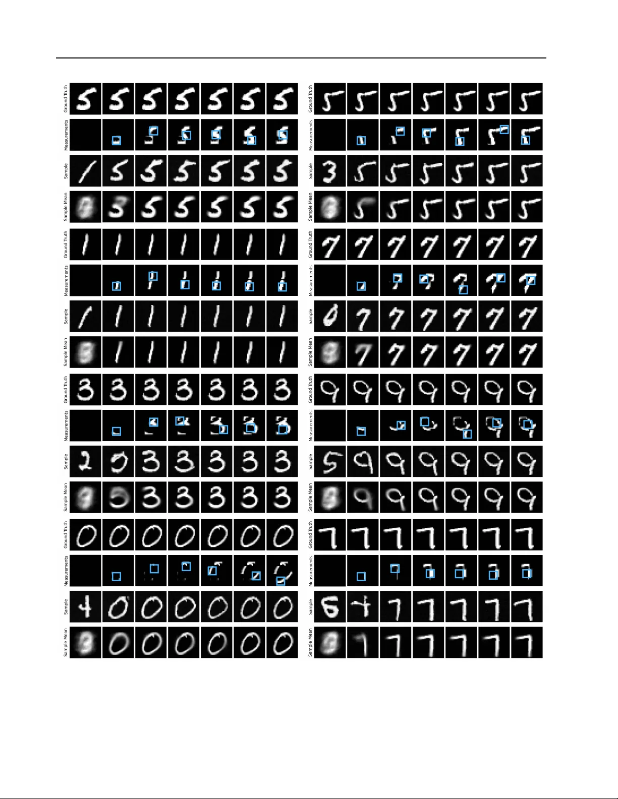
J AD AI: J ointly Amortizing Adaptive Design and Bay esian Inference Niels Bracher * 1 Lars K ¨ uhmichel * 2 Desi R. Ivanov a 3 Xavier Intes 1 Paul-Christian B ¨ urkner 2 Stefan T . Radev 1 Abstract W e consider problems of parameter estimation where design variables can be acti vely optimized to maximize information gain. T o this end, we introduce J AD AI, a frame work that jointly amor- tizes Bayesian adaptiv e design and inference by training a policy , a history network, and an in- ference network end-to-end. The networks min- imize a generic loss that aggregates incremental reductions in posterior error along e xperimental sequences. Inference networks are instantiated with diffusion-based posterior estimators that can approximate high-dimensional and multimodal posteriors at ev ery experimental step. Across standard adaptiv e design benchmarks, J AD AI achiev es superior or competitiv e performance. 1. Introduction Many scientiﬁc and engineering questions concern unob- served properties of real-world systems: cosmological parameters go verning lar ge-scale structure ( Hahn et al. , 2024 ), biophysical parameters in mechanistic neural mod- els ( Gon c ¸ alves et al. , 2020 ), or epidemiological parameters drivi ng disease dynamics ( Rade v et al. , 2021 ). In man y such settings, we can design simulators that, giv en hypothesized parameters θ , can generate synthetic observ ations x . How- ev er , in verting these simulators to recover the parameters from observations is oftentimes a computational ordeal. Simulation-based inference (SBI) addresses this in verse problem by approximating the posterior ov er parameters from simulated pairs ( θ , x ) , typically using a neural net- work ( Cranmer et al. , 2020 ; Zammit-Mangion et al. , 2025 ; Deistler et al. , 2025 ). Modern SBI employs generative mod- els, such as ﬂo w-matching ( W ildberger et al. , 2023 ), dif fu- sion ( Sharrock et al. , 2022 ), or consistency models ( Schmitt et al. , 2024 ) to represent complex, multimodal posteriors * Equal contribution 1 Rensselaer Polytechnic Institute, NY , USA 2 TU Dortmund Univ ersity , Germany 3 Univ ersity of Oxford, UK. Correspondence to: Niels Bracher < brachn@rpi.edu > , Lars K ¨ uhmichel < lars.kuehmichel@tu-dortmund.de > . Pr eprint. December 30, 2025. in high-dimensional parameter spaces ( Arruda et al. , 2025 ). Once trained, these amortized models can be applied to real observations to estimate the unobserv ed parameters. In many of these applications, howe ver , we are not only handed data, but can also actively contr ol how data is col- lected or ho w the system is perturbed. Experimental pro- tocols, stimulus sequences, or public health interventions are often parameterized by design variables ξ that strongly inﬂuence ho w informative the resulting observations x are about θ . This experimental adaptability turns the inference problem into a two-fold question: (i) ho w to infer θ from a giv en dataset, and (ii) how to choose designs ξ that make inferences as informativ e as possible. Bayesian experimental design (BED) formalizes an answer to the second question by selecting designs that maximize an expected utility , most commonly the expected information gain (EIG) about θ ( Lindley , 1956 ). In Bayesian adaptiv e design (B AD), this becomes a sequential problem in which a designer (e.g., a neural network) proposes designs based on previous decisions and data acquisitions. This idea underlies recent works on deep Bayesian adapti ve design, which learn global history-dependent policies directly from simulations ( Foster et al. , 2021 ; Iv anova et al. , 2021 ; Blau et al. , 2022 ; Huang et al. , 2025 ), rather than solving a ne w optimization problem from scratch for ev ery experiment. Despite this progress, B AD and SBI hav e largely ev olved in parallel. Policy-based B AD approaches typically focus on proposing good designs, dele gating posterior inference to slow (non-amortized) methods or restricting it to rela- tiv ely simple parametric families in low-dimensional set- tings. Con versely , SBI methods usually work with ﬁxed designs and do not directly optimize ho w observations are acquired. As a result, design and inference are typically treated as separate tasks (see Section 4 for related work). In this paper , we introduce J AD AI, a framew ork for J ointly A daptiv e D esign and A mortized Bayesian I nference. Our framew ork makes the follo wing contributions: • It jointly amortizes adapti ve e xperimental design and posterior inference via a general utility that aggreg ates incremental improv ements end-to-end. • It incorporates modern dif fusion-based generati ve mod- 1 J ADAI: J oint Adaptive Design and Amortized Inference AAAC0nicjVE7TwJBEB7OF+ALtbS5SEysCFCgJYmP2Jhg5GWQmL1jwQ33yt4eCRALY2tnqz9Mf4uF362HiQXBvezN7DfffDszawWOCFWx+JEylpZXVtfSmez6xubWdm5ntxn6kbR5w/YdX7YtFnJHeLyhhHJ4O5CcuZbDW9bwNI63RlyGwvfqahzwrssGnugLmylAtzfCjRymfHmfy5cKRb3M+U6eklXzc590Rz3yyaaIXOLkkYLvEKMQX4dKVKQAWJemwCQ8oeOcHimL3AgsDgYDOsR/gFMnQT2cY81QZ9u4xcGWyDTpEPtCK1pgx7dy+CHsF/ZEY4O5N0y1clzhGNaCYkYrXgFX9ADGokw3Yc5qWZwZd6WoTye6G4H6Ao3Efdq/OmeISGBDHTHpXDMH0LD0eYQJeLANVBBPeaZg6o57sExbrlW8RJFBT8LG00c9/3vmZrlQqhQq1+V8tZw8eJr26YCO8KrHVKVLqqEOG5W80hu9G3VjYjwZzz9UI5Xk7NGfZbx8Ay5Hkp0= Simulator AAACz3ichVFNS8NAEH3Gr9bPqkcvxSJ4KkmR6lHwAy9CC7YKbSlJ3Ma1aRKTVKlF8erNq/4z/S0efFmjoEW6YTOzb968ndmxAldGsa6/TWiTU9Mzs5ns3PzC4tJybmW1Hvn90BY123f98NwyI+FKT9RiGbviPAiF2bNccWZ195P42Y0II+l7p/EgEK2e6XiyI20zJlS/bjeDSLZzBb2oq5UfdYzUKSBdFT/3jiYu4MNGHz0IeIjpuzAR8WvAgI6AWAtDYiE9qeIC95hjbp8sQYZJtMu/w1MjRT2eE81IZdu8xeUOmZnHJveRUrTITm4V9CPaD+47hTn/3jBUykmFA1qLilmleEI8xiUZ4zJ7KfO7lvGZSVcxOthV3UjWFygk6dP+0TlgJCTWVZE8DhXToYalzjd8AY+2xgqSV/5WyKuOL2hNZYVS8VJFk3ohbfL6rIdjNv4OddSpl4pGuViubhf2SunAM1jHBrY41R3s4RgV1mHjCs94watW1W61B+3xi6pNpDlr+LW0p0+bGpE2 q ω AAAC13ichVFLS8NAEJ7GV1tfVY9egkWoICUpUj0WfOBFqGAf0lZJ0jUuzYskLdQi3sSrN6/6r/S3ePDbNRW0SDdsZvabb76d2TEDh0expr2nlJnZufmFdCa7uLS8sppbW69Hfj+0WM3yHT9smkbEHO6xWsxjhzWDkBmu6bCG2TsU8caAhRH3vYt4GLCOa9gev+GWEQO6akfcVYNCe1d8O9e5vFbU5FInHT1x8pSsqp/7oDZ1ySeL+uQSI49i+A4ZFOFrkU4aBcA6NAIWwuMyzuiessjtg8XAMID28LdxaiWoh7PQjGS2hVsc7BCZKm1jn0hFE2xxK4MfwX5i30nM/veGkVQWFQ5hTShmpOIZ8JhuwZiW6SbMcS3TM0VXMd3QgeyGo75AIqJP60fnCJEQWE9GVDqWTBsapjwP8AIebA0ViFceK6iy4y6sIS2TKl6iaEAvhBWvj3owZv3vUCedeqmol4vl8718pZQMPE2btEUFTHWfKnRKVdRhQfmFXulNuVQelEfl6ZuqpJKcDfq1lOcv1pKTLA== → p () AAAC3nichVE7SwNBEJ6c7/iKWtocBsEqbIJG0wV8YCMomEQwQfcuazxyL/Y2gRjS2omtna3+JP0tFn67XgSL4B57M/PNzLfzcGLfSxRjHxlranpmdm5+Ibu4tLyymltbrydRT7qi5kZ+JK8cngjfC0VNecoXV7EUPHB80XC6h9rf6AuZeFF4qQaxaAW8E3p3nssVoJvcRtOJ/HYyCCCGTXUvFB/d5PKsUCnt7VaYzQrMHCjaLjG7mCJ5Ss95lPukJrUpIpd6FJCgkBR0nzgl+K6pSIxiYC0aApPQPOMXNKIscnuIEojgQLv4d2Bdp2gIW3MmJtvFKz6uRKZN27gnhtFBtH5VQE8gv3AfDNaZ+MLQMOsKB5AOGBcM4xlwRfeI+C8zSCPHtfyfqbtSdEcHphsP9cUG0X26vzxH8EhgXeOx6dhEdsDhGLuPCYSQNVSgpzxmsE3HbUhupDAsYcrIwSch9fRRD9Y83qU9WamXCsVyoXyxm6+W0oXP0yZt0Q62uk9VOqVz1OFihq/0Ru/WrfVoPVnPP6FWJs3ZoD/HevkGDDyXnw== ω AAAC3nichVE7SwNBEJ6c7/iKWtocBsEqbIJG0wV8YCMomEQwQfcuazxyL/Y2gRjS2omtna3+JP0tFn67XgSL4B57M/PNzLfzcGLfSxRjHxlranpmdm5+Ibu4tLyymltbrydRT7qi5kZ+JK8cngjfC0VNecoXV7EUPHB80XC6h9rf6AuZeFF4qQaxaAW8E3p3nssVoJvcRtOJ/HYyCCCGTXUvFB/d5PKsUCnt7VaYzQrMHCjaLjG7mCJ5Ss95lPukJrUpIpd6FJCgkBR0nzgl+K6pSIxiYC0aApPQPOMXNKIscnuIEojgQLv4d2Bdp2gIW3MmJtvFKz6uRKZN27gnhtFBtH5VQE8gv3AfDNaZ+MLQMOsKB5AOGBcM4xlwRfeI+C8zSCPHtfyfqbtSdEcHphsP9cUG0X26vzxH8EhgXeOx6dhEdsDhGLuPCYSQNVSgpzxmsE3HbUhupDAsYcrIwSch9fRRD9Y83qU9WamXCsVyoXyxm6+W0oXP0yZt0Q62uk9VOqVz1OFihq/0Ru/WrfVoPVnPP6FWJs3ZoD/HevkGDDyXnw== ω AAAC03ichVFLS8NAEB7jq62vqkcvwSJ4Cmmrid4KPvAiKNgHapFN3LaheZFsizX0Il69edX/pb/Fg1/WVPBQ3LCZ2W9mvnlZoevEQtc/ZpTZufmFxVy+sLS8srpWXN9oxMEgsnndDtwgalks5q7j87pwhMtbYcSZZ7m8afWPUntzyKPYCfwrMQp522Nd3+k4NhOArm89JnpWJ3kY3xVLumbo1cNKRdW16r5xYFShmKaxZ5bVsqbLU6LsXATFT7qlewrIpgF5xMknAd0lRjG+GyqTTiGwNiXAImiOtHMaUwGxA3hxeDCgffy7eN1kqI93yhnLaBtZXNwIkSrt4J5KRgveaVYOPYb8wn2UWHdqhkQypxWOIC0w5iXjOXBBPXj8F+llnpNa/o9MuxLUoQPZjYP6Qomkfdq/PMewRMD60qLSifTsgsOS7yEm4EPWUUE65QmDKju+h2RScsniZ4wMfBFkOn3UgzVPdqlOVxoVrWxoxuVeqVbJFp6jLdqmXWzVpBqd0QXqsJHlld7oXakrifKkPP+4KjNZzCb9OcrLN0WFk3k= x fix AAAC23ichVFLT8JAEB7qC/BV9eilkZh4agoSwBuJj3gxwUQeCRDSlgU39JW2EJFw8ma8evOq/0l/iwe/roXEEMM222/2m5lvZ3YMz+JBqGmfCWlldW19I5lKb25t7+zKe/u1wB36JquaruX6DUMPmMUdVg15aLGG5zPdNixWNwbnkb8+Yn7AXecuHHusbet9h/e4qYegOrLcMlyrG4xtwKT1wKcdOaOpuWIpf5pVNLWonZW0vJJVNbHmRobiVXHlL2pRl1wyaUg2MXIohG2RTgG+JmVJIw9cmybgfFhc+BlNKY3cIaIYInSwA/z7ODVj1sE50gxEtolbLGwfmQodY18JRQPR0a0MdgD8xn4UXP/fGyZCOapwDDSgmBKKN+BDukfEskw7jpzVsjwz6iqkHpVENxz1eYKJ+jTnOhfw+OAGwqPQpYjsQ8MQ5xFewAFWUUH0yjMFRXTcBeoCmVBxYkUdej4wen3UgzEvDHXRqOXUbEEt3OYz5Vw88CQd0hGdYKpFKtM1VVCHiZre6J0+pLb0JD1LL7+hUiLOOaA/S3r9Aau2llE= ω AAAC83ichVHJSgNBEH2O+x716GUwCBEkTETUo+CCF0HBqOBImJm0sclsTk+EGPwFf8CbePXmVf9Dv8WDb9qJoiJ2011Vr6peV3W5sS9ValkvPUZvX//A4NDwyOjY+MRkYWr6UEWtxBNVL/Kj5Nh1lPBlKKqpTH1xHCfCCVxfHLnNjcx/dCkSJaPwIG3H4jRwGqE8k56TEqoVSraSgXlRs2MlzZK92N2mHci6+WUv1ApFq2zpZf5WKrlSRL72osIrbNQRwUMLAQRCpNR9OFDcJ6jAQkzsFB1iCTWp/QLXGGFui1GCEQ7RJu8GrZMcDWlnnEpne3zF50mYaWKeZ1szuozOXhXUFeUbz5XGGn++0NHMWYVtSpeMw5pxl3iKc0b8lxnkkd1a/s/MukpxhjXdjWR9sUayPr1Pnk16EmJN7TGxpSMb5HC1fckfCCmrrCD75S6DqTuuUzpaCs0S5owO+RLK7PdZD8dc+TnU38rhUrmyUl7ZXy6uL+UDH8Is5lDiVFexjh3ssQ4PN3jEE56NlnFr3Bn3H6FGT54zg2/LeHgHoj+cFw== → q ω ( | ) AAAC03ichVFLS8NAEB7jq62vqkcvwSJ4Cmmrid4KPvAiKNgHapFN3LaheZFsizX0Il69edX/pb/Fg1/WVPBQ3LCZ2W9mvnlZoevEQtc/ZpTZufmFxVy+sLS8srpWXN9oxMEgsnndDtwgalks5q7j87pwhMtbYcSZZ7m8afWPUntzyKPYCfwrMQp522Nd3+k4NhOArm89JnpWJ3kY3xVLumbo1cNKRdW16r5xYFShmKaxZ5bVsqbLU6LsXATFT7qlewrIpgF5xMknAd0lRjG+GyqTTiGwNiXAImiOtHMaUwGxA3hxeDCgffy7eN1kqI93yhnLaBtZXNwIkSrt4J5KRgveaVYOPYb8wn2UWHdqhkQypxWOIC0w5iXjOXBBPXj8F+llnpNa/o9MuxLUoQPZjYP6Qomkfdq/PMewRMD60qLSifTsgsOS7yEm4EPWUUE65QmDKju+h2RScsniZ4wMfBFkOn3UgzVPdqlOVxoVrWxoxuVeqVbJFp6jLdqmXWzVpBqd0QXqsJHlld7oXakrifKkPP+4KjNZzCb9OcrLN0WFk3k= x AAAC3nichVE7SwNBEJ6c7/iKWtocBsEqbIJG0wV8YCMomEQwQfcuazxyL/Y2gRjS2omtna3+JP0tFn67XgSL4B57M/PNzLfzcGLfSxRjHxlranpmdm5+Ibu4tLyymltbrydRT7qi5kZ+JK8cngjfC0VNecoXV7EUPHB80XC6h9rf6AuZeFF4qQaxaAW8E3p3nssVoJvcRtOJ/HYyCCCGTXUvFB/d5PKsUCnt7VaYzQrMHCjaLjG7mCJ5Ss95lPukJrUpIpd6FJCgkBR0nzgl+K6pSIxiYC0aApPQPOMXNKIscnuIEojgQLv4d2Bdp2gIW3MmJtvFKz6uRKZN27gnhtFBtH5VQE8gv3AfDNaZ+MLQMOsKB5AOGBcM4xlwRfeI+C8zSCPHtfyfqbtSdEcHphsP9cUG0X26vzxH8EhgXeOx6dhEdsDhGLuPCYSQNVSgpzxmsE3HbUhupDAsYcrIwSch9fRRD9Y83qU9WamXCsVyoXyxm6+W0oXP0yZt0Q62uk9VOqVz1OFihq/0Ru/WrfVoPVnPP6FWJs3ZoD/HevkGDDyXnw== ω AAAC3nichVE7SwNBEJ6c7/iKWtocBsEqbIJG0wV8YCMomEQwQfcuazxyL/Y2gRjS2omtna3+JP0tFn67XgSL4B57M/PNzLfzcGLfSxRjHxlranpmdm5+Ibu4tLyymltbrydRT7qi5kZ+JK8cngjfC0VNecoXV7EUPHB80XC6h9rf6AuZeFF4qQaxaAW8E3p3nssVoJvcRtOJ/HYyCCCGTXUvFB/d5PKsUCnt7VaYzQrMHCjaLjG7mCJ5Ss95lPukJrUpIpd6FJCgkBR0nzgl+K6pSIxiYC0aApPQPOMXNKIscnuIEojgQLv4d2Bdp2gIW3MmJtvFKz6uRKZN27gnhtFBtH5VQE8gv3AfDNaZ+MLQMOsKB5AOGBcM4xlwRfeI+C8zSCPHtfyfqbtSdEcHphsP9cUG0X26vzxH8EhgXeOx6dhEdsDhGLuPCYSQNVSgpzxmsE3HbUhupDAsYcrIwSch9fRRD9Y83qU9WamXCsVyoXyxm6+W0oXP0yZt0Q62uk9VOqVz1OFihq/0Ru/WrfVoPVnPP6FWJs3ZoD/HevkGDDyXnw== ω AAACz3ichVFNS8NAEH3Gr9bPqkcvxSJ4KkmR6lHwAy9CC7YKbSlJ3Ma1aRKTVKlF8erNq/4z/S0efFmjoEW6YTOzb968ndmxAldGsa6/TWiTU9Mzs5ns3PzC4tJybmW1Hvn90BY123f98NwyI+FKT9RiGbviPAiF2bNccWZ195P42Y0II+l7p/EgEK2e6XiyI20zJlS/bjeDSLZzBb2oq5UfdYzUKSBdFT/3jiYu4MNGHz0IeIjpuzAR8WvAgI6AWAtDYiE9qeIC95hjbp8sQYZJtMu/w1MjRT2eE81IZdu8xeUOmZnHJveRUrTITm4V9CPaD+47hTn/3jBUykmFA1qLilmleEI8xiUZ4zJ7KfO7lvGZSVcxOthV3UjWFygk6dP+0TlgJCTWVZE8DhXToYalzjd8AY+2xgqSV/5WyKuOL2hNZYVS8VJFk3ohbfL6rIdjNv4OddSpl4pGuViubhf2SunAM1jHBrY41R3s4RgV1mHjCs94watW1W61B+3xi6pNpDlr+LW0p0+bGpE2 q ω AAAC0XichVFNT8JAEB3qF+AX6tFLIzHxRAoH9EgiGi8mGEVIkJhtWeqGfmVbSJCYGK/evOof09/iwbdrMVFi2GY7s2/evJ3ZsSNPxIllvWeMhcWl5ZVsLr+6tr6xWdjavo7DoXR40wm9ULZtFnNPBLyZiMTj7Uhy5tseb9mDYxVvjbiMRRhcJeOId33mBqIvHJYAatd5LNyAy9tC0SpZepmzTjl1ipSuRlj4oBvqUUgODcknTgEl8D1iFOPrUJksioB1aQJMwhM6zumB8sgdgsXBYEAH+Ls4dVI0wFlpxjrbwS0etkSmSfvYp1rRBlvdyuHHsJ/Y9xpz/71hopVVhWNYG4o5rXgOPKE7MOZl+ilzWsv8TNVVQn060t0I1BdpRPXp/OjUEZHABjpi0olmutCw9XmEFwhgm6hAvfJUwdQd92CZtlyrBKkig56EVa+PejDm8t+hzjrXlVK5WqpeVIq1SjrwLO3SHh1gqodUozNqoA41zRd6pTfj0hgbj8bTN9XIpDk79GsZz1+ma5IB Designer AAAC13ichVFLS8NAEJ7GV1tfVY9egkWoICUpUj0WfOBFqGAf0lZJ0jUuzYskLdQi3sSrN6/6r/S3ePDbNRW0SDdsZvabb76d2TEDh0expr2nlJnZufmFdCa7uLS8sppbW69Hfj+0WM3yHT9smkbEHO6xWsxjhzWDkBmu6bCG2TsU8caAhRH3vYt4GLCOa9gev+GWEQO6akfcVYNCe1d8O9e5vFbU5FInHT1x8pSsqp/7oDZ1ySeL+uQSI49i+A4ZFOFrkU4aBcA6NAIWwuMyzuiessjtg8XAMID28LdxaiWoh7PQjGS2hVsc7BCZKm1jn0hFE2xxK4MfwX5i30nM/veGkVQWFQ5hTShmpOIZ8JhuwZiW6SbMcS3TM0VXMd3QgeyGo75AIqJP60fnCJEQWE9GVDqWTBsapjwP8AIebA0ViFceK6iy4y6sIS2TKl6iaEAvhBWvj3owZv3vUCedeqmol4vl8718pZQMPE2btEUFTHWfKnRKVdRhQfmFXulNuVQelEfl6ZuqpJKcDfq1lOcv1pKTLA== → p () AAAC3nichVE7SwNBEJ6c7/iKWtocBsEqbIJG0wV8YCMomEQwQfcuazxyL/Y2gRjS2omtna3+JP0tFn67XgSL4B57M/PNzLfzcGLfSxRjHxlranpmdm5+Ibu4tLyymltbrydRT7qi5kZ+JK8cngjfC0VNecoXV7EUPHB80XC6h9rf6AuZeFF4qQaxaAW8E3p3nssVoJvcRtOJ/HYyCCCGTXUvFB/d5PKsUCnt7VaYzQrMHCjaLjG7mCJ5Ss95lPukJrUpIpd6FJCgkBR0nzgl+K6pSIxiYC0aApPQPOMXNKIscnuIEojgQLv4d2Bdp2gIW3MmJtvFKz6uRKZN27gnhtFBtH5VQE8gv3AfDNaZ+MLQMOsKB5AOGBcM4xlwRfeI+C8zSCPHtfyfqbtSdEcHphsP9cUG0X26vzxH8EhgXeOx6dhEdsDhGLuPCYSQNVSgpzxmsE3HbUhupDAsYcrIwSch9fRRD9Y83qU9WamXCsVyoXyxm6+W0oXP0yZt0Q62uk9VOqVz1OFihq/0Ru/WrfVoPVnPP6FWJs3ZoD/HevkGDDyXnw== ω AAAC3nichVE7SwNBEJ6c7/iKWtocBsEqbIJG0wV8YCMomEQwQfcuazxyL/Y2gRjS2omtna3+JP0tFn67XgSL4B57M/PNzLfzcGLfSxRjHxlranpmdm5+Ibu4tLyymltbrydRT7qi5kZ+JK8cngjfC0VNecoXV7EUPHB80XC6h9rf6AuZeFF4qQaxaAW8E3p3nssVoJvcRtOJ/HYyCCCGTXUvFB/d5PKsUCnt7VaYzQrMHCjaLjG7mCJ5Ss95lPukJrUpIpd6FJCgkBR0nzgl+K6pSIxiYC0aApPQPOMXNKIscnuIEojgQLv4d2Bdp2gIW3MmJtvFKz6uRKZN27gnhtFBtH5VQE8gv3AfDNaZ+MLQMOsKB5AOGBcM4xlwRfeI+C8zSCPHtfyfqbtSdEcHphsP9cUG0X26vzxH8EhgXeOx6dhEdsDhGLuPCYSQNVSgpzxmsE3HbUhupDAsYcrIwSch9fRRD9Y83qU9WamXCsVyoXyxm6+W0oXP0yZt0Q62uk9VOqVz1OFihq/0Ru/WrfVoPVnPP6FWJs3ZoD/HevkGDDyXnw== ω AAAC1XichVFLT8JAEB7qC/CFevTSSEw8kRYF9UbiI15MMOGVACHbskBDX2kXEiTcjFdvXvVv6W/x4Ne1mBhD2GY7s9988+3MjuHbVig07SOhrKyurW8kU+nNre2d3czefi30RoHJq6Zne0HDYCG3LZdXhSVs3vADzhzD5nVjeBXF62MehJbnVsTE522H9V2rZ5lMAGq1HCYGRm86mHUqnUxWyxUK2qV+qv539JwmV5biVfYyn9SiLnlk0ogc4uSSgG8ToxBfk3TSyAfWpimwAJ4l45xmlEbuCCwOBgM6xL+PUzNGXZwjzVBmm7jFxg6QqdIx9q1UNMCObuXwQ9gv7EeJ9RfeMJXKUYUTWAOKKal4D1zQAIxlmU7MnNeyPDPqSlCPLmQ3FurzJRL1af7qXCMSABvKiEo3ktmHhiHPY7yAC1tFBdErzxVU2XEXlknLpYobKzLoBbDR66MejHk+S3WxU8vn9GKu+HCWLeXjgSfpkI7oBFM9pxLdURl1mOjjld7oXakrM+VJef6hKok454D+LOXlG/v3lCA= h T AAAC+3ichVHJSgNBEH2O+x716GUwCAoSJkHUY8AFL4KCUcGRMDNpY5PZnJ4IUfwNf8CbePXmVf9Bv8WDb9qJoiJ2011Vr6peV3W5sS9ValkvPUZvX//A4NDwyOjY+MRkYWr6QEXtxBM1L/Kj5Mh1lPBlKGqpTH1xFCfCCVxfHLqt9cx/eCESJaNwP+3E4iRwmqE8lZ6TEqoXLNNWMjDP63as5IK91N2mHciG+WV392K9ULRKll7mb6WcK0XkazcqvMJGAxE8tBFAIERK3YcDxX2MMizExE5wRSyhJrVf4BojzG0zSjDCIdri3aR1nKMh7YxT6WyPr/g8CTNNzPNsaUaX0dmrgrqifOO51FjzzxeuNHNWYYfSJeOwZtwhnuKMEf9lBnlkt5b/M7OuUpxiTXcjWV+skaxP75Nng56EWEt7TGzqyCY5XG1f8AdCyhoryH65y2DqjhuUjpZCs4Q5o0O+hDL7fdbDMZd/DvW3clAplVdKK3vLxWolH/gQZjGHBU51FVVsY5d1eLjBI57wbFwbt8adcf8RavTkOTP4toyHd1Gjnoc= → q ω ( | ) AAAC3nichVE7SwNBEJ6c7/iKWtocBsEqbIJG0wV8YCMomEQwQfcuazxyL/Y2gRjS2omtna3+JP0tFn67XgSL4B57M/PNzLfzcGLfSxRjHxlranpmdm5+Ibu4tLyymltbrydRT7qi5kZ+JK8cngjfC0VNecoXV7EUPHB80XC6h9rf6AuZeFF4qQaxaAW8E3p3nssVoJvcRtOJ/HYyCCCGTXUvFB/d5PKsUCnt7VaYzQrMHCjaLjG7mCJ5Ss95lPukJrUpIpd6FJCgkBR0nzgl+K6pSIxiYC0aApPQPOMXNKIscnuIEojgQLv4d2Bdp2gIW3MmJtvFKz6uRKZN27gnhtFBtH5VQE8gv3AfDNaZ+MLQMOsKB5AOGBcM4xlwRfeI+C8zSCPHtfyfqbtSdEcHphsP9cUG0X26vzxH8EhgXeOx6dhEdsDhGLuPCYSQNVSgpzxmsE3HbUhupDAsYcrIwSch9fRRD9Y83qU9WamXCsVyoXyxm6+W0oXP0yZt0Q62uk9VOqVz1OFihq/0Ru/WrfVoPVnPP6FWJs3ZoD/HevkGDDyXnw== ω AAAC3nichVE7SwNBEJ6c7/iKWtocBsEqbIJG0wV8YCMomEQwQfcuazxyL/Y2gRjS2omtna3+JP0tFn67XgSL4B57M/PNzLfzcGLfSxRjHxlranpmdm5+Ibu4tLyymltbrydRT7qi5kZ+JK8cngjfC0VNecoXV7EUPHB80XC6h9rf6AuZeFF4qQaxaAW8E3p3nssVoJvcRtOJ/HYyCCCGTXUvFB/d5PKsUCnt7VaYzQrMHCjaLjG7mCJ5Ss95lPukJrUpIpd6FJCgkBR0nzgl+K6pSIxiYC0aApPQPOMXNKIscnuIEojgQLv4d2Bdp2gIW3MmJtvFKz6uRKZN27gnhtFBtH5VQE8gv3AfDNaZ+MLQMOsKB5AOGBcM4xlwRfeI+C8zSCPHtfyfqbtSdEcHphsP9cUG0X26vzxH8EhgXeOx6dhEdsDhGLuPCYSQNVSgpzxmsE3HbUhupDAsYcrIwSch9fRRD9Y83qU9WamXCsVyoXyxm6+W0oXP0yZt0Q62uk9VOqVz1OFihq/0Ru/WrfVoPVnPP6FWJs3ZoD/HevkGDDyXnw== ω AAAC1XichVFLT8JAEB7qC/CFevTSSEw8kRYF9UbiI15MMOGVACHbskBDX2kXEiTcjFdvXvVv6W/x4Ne1mBhD2GY7s9988+3MjuHbVig07SOhrKyurW8kU+nNre2d3czefi30RoHJq6Zne0HDYCG3LZdXhSVs3vADzhzD5nVjeBXF62MehJbnVsTE522H9V2rZ5lMAGq1HCYGRm86mHUqnUxWyxUK2qV+qv539JwmV5biVfYyn9SiLnlk0ogc4uSSgG8ToxBfk3TSyAfWpimwAJ4l45xmlEbuCCwOBgM6xL+PUzNGXZwjzVBmm7jFxg6QqdIx9q1UNMCObuXwQ9gv7EeJ9RfeMJXKUYUTWAOKKal4D1zQAIxlmU7MnNeyPDPqSlCPLmQ3FurzJRL1af7qXCMSABvKiEo3ktmHhiHPY7yAC1tFBdErzxVU2XEXlknLpYobKzLoBbDR66MejHk+S3WxU8vn9GKu+HCWLeXjgSfpkI7oBFM9pxLdURl1mOjjld7oXakrM+VJef6hKok454D+LOXlG/v3lCA= h T AAAC0nicjVE7TwJBEB7OF+ALtbS5SEysCFCgJYmP2Jhg5GWQmL1jwQ33yt4eCRALY2tnqz9Mf4uF362HiQXBvezN7DfffDszawWOCFWx+JEylpZXVtfSmez6xubWdm5ntxn6kbR5w/YdX7YtFnJHeLyhhHJ4O5CcuZbDW9bwNI63RlyGwvfqahzwrssGnugLmylAtzfCjRymfHmfy5cKRb3M+U6eklXzc590Rz3yyaaIXOLkkYLvEKMQX4dKVKQAWJemwCQ8oeOcHimL3AgsDgYDOsR/gFMnQT2cY81QZ9u4xcGWyDTpEPtCK1pgx7dy+CHsF/ZEY4O5N0y1clzhGNaCYkYrXgFX9ADGokw3Yc5qWZwZd6WoTye6G4H6Ao3Efdq/OmeISGBDHTHpXDMH0LD0eYQJeLANVBBPeaZg6o57sExbrlW8RJFBT8LG00c9/3vmZrlQqhQq1+V8tZw8eJr26YCO8KrHVKVLqqEOG5W80hu9G3VjYjwZzz9UI5Xk7NGfZbx8Ay5Hkp0= Simulator AAAC1HichVFLS8NAEJ7GV+uz6tFLsAieSlKkeiz4wItQwT6gLWWTbmNoXiTbQq2exKs3r/q79Ld48Ns1FbRIN2xm9ptvvp3ZsSLPTYRhvGe0hcWl5ZVsbnVtfWNzK7+9U0/CYWzzmh16Ydy0WMI9N+A14QqPN6OYM9/yeMManMp4Y8TjxA2DGzGOeMdnTuD2XZsJQK02F6zbDn3usG6+YBQNtfRZx0ydAqWrGuY/qE09CsmmIfnEKSAB3yNGCb4WmWRQBKxDE2AxPFfFOT3QKnKHYHEwGNAB/g5OrRQNcJaaicq2cYuHHSNTpwPsC6VogS1v5fAT2E/sO4U5/94wUcqywjGsBcWcUrwCLugWjHmZfsqc1jI/U3YlqE8nqhsX9UUKkX3aPzpniMTABiqi07liOtCw1HmEFwhga6hAvvJUQVcd92CZslypBKkig14MK18f9WDM5t+hzjr1UtEsF8vXR4VKKR14lvZonw4x1WOq0CVVUYecywu90ptW1+61R+3pm6pl0pxd+rW05y/sI5NK ω ω AAAC0XichVFLS8NAEJ7GV1tfVY9egkXwVJIi1WPBB16EivYBbSlJum2X5kWyLdQiiFdvXvWP6W/x4LdrKmiRbtjM7DfffDuzY4cuj4VhvKe0peWV1bV0Jru+sbm1ndvZrcXBKHJY1QncIGrYVsxc7rOq4MJljTBilme7rG4Pz2S8PmZRzAP/TkxC1vasvs973LEEoEYr5J1WOOCdXN4oGGrp846ZOHlKViXIfVCLuhSQQyPyiJFPAr5LFsX4mmSSQSGwNk2BRfC4ijN6oCxyR2AxMCygQ/z7ODUT1MdZasYq28EtLnaETJ0OsS+Vog22vJXBj2E/se8V1v/3hqlSlhVOYG0oZpTiNXBBAzAWZXoJc1bL4kzZlaAenapuOOoLFSL7dH50zhGJgA1VRKcLxexDw1bnMV7Ah62iAvnKMwVdddyFtZRlSsVPFC3oRbDy9VEPxmz+Heq8UysWzFKhdHOcLxeTgadpnw7oCFM9oTJdUQV1yGm+0Cu9abfaRHvUnr6pWirJ2aNfS3v+AqeBkgM= ω ω AAAC0HichVFLSwMxEJ6u7/qqevSyWARPS1pLW2+CD7wIVVortEV211hD98UmFR+IePXmVX+Z/hYPfolbQUTMkp3JN998mcl4SSCkYuwtZ42NT0xOTc/kZ+fmFxYLS8snMh6mPm/5cRCnp54reSAi3lJCBfw0SbkbegFve4MdHW9f8VSKOGqqm4T3QrcfiQvhuwpQu9lVIuTyrFBkTrlWr2yWbObU2FadVeySw8z6doqUrUZceKcunVNMPg0pJE4RKfgBuSTxdahEjBJgPboDlsITJs7pnvLIHYLFwXCBDvDv49TJ0AhnrSlNto9bAuwUmTatY+8bRQ9sfSuHL2E/sG8N1v/zhjujrCu8gfWgOGMUD4ErugTjv8wwY45q+T9Td6XoguqmG4H6EoPoPv1vnV1EUmADE7FpzzD70PDM+QovEMG2UIF+5ZGCbTo+h3WN5UYlyhRd6KWw+vVRD8b8a6i/nZOyU6o61aNKcbucDXyaVmmNNjDVGm3TATVQh+7wmV7o1Tq2rq0H6/GLauWynBX6saynTxmckdA= T → AAAC1XichVFLS8NAEJ7Gd31VPXoJFsFTSB+m9Sb4wItQwT6gLWWTbtvQvEi2RS29iVdvXvVv6W/x4Jc1FTyUbtjM7DfffDuzYwaOHQld/0wpS8srq2vrG+nNre2d3czefi3yR6HFq5bv+GHDZBF3bI9XhS0c3ghCzlzT4XVzeBHH62MeRrbv3YvHgLdd1vfsnm0xAajVcpkYmL3Jw7QjOpmsrhl64SyfV3WtcGqUjQKcUskolnJqTtPlylKyKn7mi1rUJZ8sGpFLnDwS8B1iFOFrUo50CoC1aQIshGfLOKcppZE7AouDwYAO8e/j1ExQD+dYM5LZFm5xsENkqnSMfS0VTbDjWzn8CPYb+0li/bk3TKRyXOEjrAnFDal4C1zQAIxFmW7CnNWyODPuSlCPyrIbG/UFEon7tP50LhEJgQ1lRKUryexDw5TnMV7Ag62igviVZwqq7LgLy6TlUsVLFBn0Qtj49VEPxjybpTrfqeW1nKEZd8XseT4Z+Dod0hGdYKolOqcbqqAOC3280Tt9KHVlqjwrL79UJZXkHNC/pbz+AJRClGA= x t AAAC3XichVFNS8NAEH3G7++qRy/BIngKaS1tvQl+4EVQsCpYKUm61qX5ItmKtXj0Jl69edW/pL/Fgy9rFETEDZuZffPm7cyOG/syVbb9OmQMj4yOjU9MTk3PzM7NFxYWj9Ool3ii4UV+lJy6Tip8GYqGksoXp3EinMD1xYnb3criJ1ciSWUUHql+LM4DpxPKC+k5ilCrsNh0I7+d9gOaQfNa3rZUq1C0rXKtXlkvmbZVszfqdsUsWbZe304R+TqICm9ooo0IHnoIIBBC0ffhIOV3hhJsxMTOMSCW0JM6LnCLKeb2yBJkOES7/Hd4OsvRkOdMM9XZHm/xuRNmmljl3tWKLtnZrYJ+SvvOfaOxzp83DLRyVmGf1qXipFbcJ65wScZ/mUHO/Krl/8ysK4UL1HU3kvXFGsn69L51thlJiHV1xMSOZnao4erzFV8gpG2wguyVvxRM3XGb1tFWaJUwV3Sol9Bmr896OOZfQ/3tHJetUtWqHlaKm+V84BNYxgrWONUaNrGHA9bh4RpPeMaL0TLujHvj4ZNqDOU5S/ixjMcP/92XOA== ω t fix AAAC1nichVHLSsNAFD3GV+uz6tJNsAiuSqrWx67gg24EBasFLTKJYw3Ny2Qq1FJ34tadW/0s/RYXnoypICJOmNw755575t65duS5ibKstyFjeGR0bDyXn5icmp6ZLczNnyRhJ3Zk3Qm9MG7YIpGeG8i6cpUnG1EshW978tRu76Tx01sZJ24YHKtuJJu+aAXulesIRah57gt17QivV+tfHF8UilapUrG2y2vmb6dcsvQqIluHYeEd57hECAcd+JAIoOh7EEj4naEMCxGxJnrEYnqujkv0McHcDlmSDEG0zX+Lp7MMDXhONROd7fAWjztmpoll7n2taJOd3irpJ7Qf3Hcaa/15Q08rpxV2aW0q5rXiAXGFazL+y/Qz5qCW/zPTrhSusKW7cVlfpJG0T+dbZ5eRmFhbR0zsaWaLGrY+3/IFAto6K0hfeaBg6o4vaYW2UqsEmaKgXkybvj7r4ZgHszT/dk5WS+WN0sbRerG6mg08h0UsYYVT3UQVNRyyDgc3eMYLXo2GcW88GI9fVGMoy1nAj2U8fQLTBZRy H T AAAC3nichVE7SwNBEJ6c7/iKWtocBsEqbIJG0wV8YCMomEQwQfcuazxyL/Y2gRjS2omtna3+JP0tFn67XgSL4B57M/PNzLfzcGLfSxRjHxlranpmdm5+Ibu4tLyymltbrydRT7qi5kZ+JK8cngjfC0VNecoXV7EUPHB80XC6h9rf6AuZeFF4qQaxaAW8E3p3nssVoJvcRtOJ/HYyCCCGTXUvFB/d5PKsUCnt7VaYzQrMHCjaLjG7mCJ5Ss95lPukJrUpIpd6FJCgkBR0nzgl+K6pSIxiYC0aApPQPOMXNKIscnuIEojgQLv4d2Bdp2gIW3MmJtvFKz6uRKZN27gnhtFBtH5VQE8gv3AfDNaZ+MLQMOsKB5AOGBcM4xlwRfeI+C8zSCPHtfyfqbtSdEcHphsP9cUG0X26vzxH8EhgXeOx6dhEdsDhGLuPCYSQNVSgpzxmsE3HbUhupDAsYcrIwSch9fRRD9Y83qU9WamXCsVyoXyxm6+W0oXP0yZt0Q62uk9VOqVz1OFihq/0Ru/WrfVoPVnPP6FWJs3ZoD/HevkGDDyXnw== ω AAAC23ichVFLS8NAEB7j+x316CVYBC+WpNqqN8EHXgQFq4KWsptu09C82GwFDT15E6/evOp/0t/iwS9rKoiIGzYz+803387s8CTwU2Xbb0PG8Mjo2PjE5NT0zOzcvLmweJ7GPemKuhsHsbzkLBWBH4m68lUgLhMpWMgDccG7e3n84kbI1I+jM3WbiEbIvMhv+y5TgJqmeR0y1eHtrNNvZmrd6TfNkl2uVu0dZ8P67ThlW68SFeskNt/pmloUk0s9CklQRAp+QIxSfFfkkE0JsAZlwCQ8X8cF9WkKuT2wBBgMaBd/D6erAo1wzjVTne3ilgBbItOiVexDrcjBzm8V8FPYD+w7jXl/3pBp5bzCW1gOxUmteAxcUQeM/zLDgjmo5f/MvCtFbdrW3fioL9FI3qf7rbOPiATW1RGLDjTTgwbX5xu8QARbRwX5Kw8ULN1xC5ZpK7RKVCgy6EnY/PVRD8Y8mKX1t3NeKTu1cu10s7RbKQY+Qcu0QmuY6hbt0hGdoA4XNT3TC70aDePeeDAev6jGUJGzRD+W8fQJvfuV7w== h t → 1 Amortized Inference Adaptive Desig n J AD AI Observat ion Experimental Design Prior Poster ior Hist ory F igur e 1. Ov erview of amortized SBI, B AD, and our proposed J AD AI frame work. Left: Amortized SBI, where a neural posterior estimator q ψ ( θ | x ) is trained on simulator pairs ( x , θ ) under a ﬁx ed design ξ . Middle: Amortized B AD, where a designer runs a full T -step rollout for a ﬁxed parameter θ : a policy π ϕ maps the history state h t − 1 = η ω ( { ( ξ k , x k ) } t − 1 k =1 ) to a new design ξ t , and the simulator returns x t , iterativ ely forming the history H T = { ( ξ t , x t ) } T t =1 . Right: J AD AI embeds this designer (middle block) into the amortized SBI loop and jointly trains π ϕ , η ω , and q ψ end-to-end, amortizing both experimental design and posterior inference across rollouts and e xperiments. els, providing amortized high-dimensional and multi- modal posteriors at ev ery experimental step. • It achiev es superior or competitive performance across a range of adaptiv e design benchmarks. 2. Background 2.1. Simulators as statistical models For the purpose of our discussion, a simulator generates observables x ∈ X as a function of unknown parameters θ ∈ Θ , design v ariables ξ ∈ Ξ and random program states z ∈ Z : x = Sim( θ , z ; ξ ) with θ ∼ p ( θ ) , z ∼ RNG( · ) (1) The forward pr oblem in ( 1 ) is typically well-understood through a mathematical model. The in verse pr oblem , ho w- ev er , is typically much harder , and forms the crux of Bayesian inference: for a given design ξ , estimate the un- knowns θ from observables x via the posterior distribution : p ( θ | x ; ξ ) ∝ p ( θ ) p ( x | θ ; ξ ) . (2) Howe ver , when w orking with complex simulators, the like- lihood p ( x | θ , ξ ) needed for proper statistical inference cannot be directly ev aluated. In these cases, a posterior esti- mator q ( θ | x ; ξ ) needs to be constructed from simulations of ( 1 ) alone. This is the gist of simulation-based inference (SBI; Cranmer et al. , 2020 ; Diggle & Gratton , 1984 ). 2.2. Neural simulation-based inference In neural SBI, synthetic pairs ( θ n , x n ) obtained via ( 1 ) are used to train a (generative) neural network. The network can approximate either the intractable posterior , likelihood, or both. The network is then applied to unlabeled real observations x o , essentially solving a sim2real problem. Neural SBI is compatible with any of f-the-shelf generativ e model, such as normalizing ﬂows ( Rezende & Mohamed , 2015 ), ﬂow matching ( Lipman et al. , 2023 ), or diffusion models ( Song & Ermon , 2019 ). In this work, we focus speciﬁcally on amortized methods , which train a single (global) posterior estimator q ( θ | x ; ξ ) that remains valid for any x o ∼ p ∗ ( x o ) (see Figure 1 , left ). 2.3. Bayesian experimental design SBI methods are typically de veloped and applied for a ﬁxed design ξ . Ideally , we want to choose the design that maxi- mizes the amount of information we expect to gain from our subsequent observ ations. This is the goal of Bayesian e xper- imental design (BED; Lindley , 1956 ; Chaloner & V erdinelli , 1995 ; Rainforth et al. , 2024 ). Realized information gain. Suppose we run an experi- ment with design ξ and obtain an actual observation x o . The r ealized information gain (IG) is deﬁned as the reduction in entropy from the prior p ( θ ) to the posterior p ( θ | x o ; ξ ) : IG( x o , ξ ) := H [ p ( θ )] − H [ p ( θ | x o ; ξ )] , (3) where H [ p ] denotes the Shannon entropy of p . Crucially , the IG can be ev aluated only after observing the outcome x o and ﬁtting a posterior p ( θ | x o ; ξ ) . Expected information gain. Before running the exper - iment, ho wever , the outcome x is unknown. Thus, the realized IG ( 3 ) cannot be used to select a design ξ . Instead, BED aims to select the design that maximizes the expected information gain (EIG), where the expectation is taken with respect to the prior predictive distrib ution of the outcome, p ( x | ξ ) = R p ( x | θ , ξ ) p ( θ ) d θ : EIG( ξ ) : = E p ( x | ξ ) [IG( x , ξ )] (4) = E p ( θ ) p ( x | θ , ξ ) [log p ( θ | x ; ξ ) − log p ( θ )] (5) The second expression shows that EIG( ξ ) is the mutual information between θ and x under design ξ . Maximizing 2 J ADAI: J oint Adaptive Design and Amortized Inference the EIG, therefore, selects designs that, on averag e , are expected to yield the most informati ve observ ations about θ . 2.4. Bayesian adaptiv e design BED is particularly attractiv e when experiments entail a sequence of design decisions ξ 1 , . . . , ξ T , where each deci- sion can mak e use of pre vious observ ations ( Rainforth et al. , 2024 ). Let H t − 1 = { ( ξ k , x k ) } t − 1 k =1 denote the raw experi- mental history up to step t . At each such step, we can update our beliefs p ( θ | H t − 1 ) based on all information gathered so far , and then choose the next design ξ t by maximizing the incr emental expected information gain: EIG( ξ t | H t − 1 ) := E p ( θ |H t − 1 ) p ( x t | θ , ξ t )  log p ( θ | H t − 1 , x t ; ξ t ) p ( θ | H t − 1 )  . (6) This expression is simply the standard EIG ( 5 ) , but ev aluated using the current posterior as the prior for the next step. Thus, B AD selects designs by maximizing ( 6 ) at each step t , with H 0 = ∅ (see Figure 1 , middle ). Foster et al. ( 2021 ) introduced a policy network π ϕ that predicts the next design from history , π ϕ ( H t − 1 ) = ξ t , and showed that the decision process can be amortized ov er all T steps by maximizing the total EIG (TEIG): TEIG( π ϕ ) := E " T X t =1 EIG  π ϕ ( H t − 1 ) | H t − 1  # (7) = E [log p ( H T | θ , π ϕ ) − log p ( H T | π ϕ )] (8) = E [log p ( θ | H T , π ϕ ) − log p ( θ )] , (9) where all expectations are under p ( θ ) p ( H T | θ , π ϕ ) . In the next section, we extend this framew ork to the typical SBI setting, and jointly amortize both the design policy and posterior inference across experimental time. 3. Method 3.1. Setup Our framework builds on the SBI and BAD setting from Sec- tion 2 (see also Figure 1 , right ). T o represent the history in a ﬁxed-dimensional form, we introduce a summary network η ω that maps the history sequence H t = { ( ξ k , x k ) } t k =1 to a summary statistic h t = η ω  H t  , t = 0 , . . . , T , (10) with h 0 = 0 corresponding to the empty history state. As in amortized policy-based B AD ( F oster et al. , 2021 ; Ivano va et al. , 2021 ), a deterministic polic y network π ϕ selects the next design based on the current summary , ξ t = π ϕ ( h t − 1 ) at each step t ≥ 1 . Inference is performed by a neural posterior estimator q ψ ( θ | h t ) , which takes the summary h t as input and approximates the intractable posterior p ( θ | h t ) . For a simulated pair ( θ , h t ) we deﬁne the per -step training loss ℓ t ( θ , h t ; ϕ, ω , ψ ) := L post ( θ , h t ; ϕ, ω , ψ ) , (11) where L post is the posterior loss induced by the posterior estimator (e.g., score matching or ﬂo w matching; see Sec- tion A.1 and Section A.2 for details). Although q ψ is the only density estimator , ℓ t depends on all parameters ( ϕ, ω , ψ ) through the summary h t = η ω ( { ( ξ k , x k ) } t k =1 ) and the designs ξ k = π ϕ ( h k − 1 ) . W e treat ℓ t as a shared training signal to update the policy π ϕ , the summary net- work η ω , and the posterior estimator q ψ . For notational con venience, we will usually suppress the explicit depen- dence on ( ϕ, ω , ψ ) and write ℓ t instead of ℓ t ( θ , h t ; ϕ, ω , ψ ) . 3.2. Optimization objective T o obtain a tractable training objecti ve, we use the Barber - Agako v variational lo wer bound ( Barber & Agako v , 2003 ; Foster et al. , 2019 ; Blau et al. , 2023 ) and replace the true posterior p ( θ | h T ) by a neural estimator q ψ ( θ | h T ) in ( 9 ) : TEIG( π ϕ ) ≥ E p ( θ , h T | π ϕ ,η ω )  log q ψ ( θ | h T ) p ( θ )  , (12) with equality if and only if q ψ ( θ | h T ) = p ( θ | h T ) almost ev erywhere. For intuition, we ﬁrst consider the case when q ψ is a normalized density model, i.e., a normalizing ﬂow with ℓ ﬂow t ( θ , h t ) := − log q ψ ( θ | h t ) as in Blau et al. ( 2023 ). Then the logarithm in ( 12 ) admits the decomposition log q ψ ( θ | h T ) p ( θ ) = T X t =1 log q ψ ( θ | h t ) q ψ ( θ | h t − 1 ) (13) = T X t =1 ℓ ﬂow t − 1 − ℓ ﬂow t . (14) Hence, for a normalized density model, the variational TEIG bound can be written as a telescoping sum of per-step dif fer- ences in information content. Howe ver , the use of normaliz- ing ﬂows can be restricti ve in practice ( Chen et al. , 2025 ), and we want our framew ork to generalize beyond inference models with exact log-density computation. Thus, we suggest using the generic quantity ℓ t − 1 − ℓ t as a proxy for the incremental information gained from step t − 1 to t , ev en when q ψ is approximated with an implicit model for which the normalized log-posterior is not directly av ailable. For example, a diffusion model formulation of ( 14 ) entails the difference in posterior scores as a summand: ∇ θ τ log p ( θ τ | h t − 1 ) − ∇ θ τ log p ( θ τ | h t ) , (15) 3 J ADAI: J oint Adaptive Design and Amortized Inference where τ denotes diffusion time (see Section A.1 ). In that case, the Barber–Agak ov interpretation ( Barber & Agako v , 2003 ) is no longer the same, b ut the resulting objective still encourages trajectories along which the posterior loss decreases, as demonstrated by our experiments in Section 5 . This motiv ates the deﬁnition of the general scalar utility u T ( θ , h 0: T ) := T X t =0  ℓ ∗ t − 1 − ℓ t  , ℓ − 1 := 0 , (16) where ℓ ∗ t = detach ( ℓ t ) denotes the same loss v alue with gradients stopped. Our ﬁnal training objectiv e minimizes the negati ve e xpected utility L ( ϕ, ψ , ω ) := E p ( θ ) p ( h 0: T | θ ,π ϕ ,η ω )  − u T ( θ , h 0: T )  , (17) using mini-batch gradient descent on L . Since the sum in ( 16 ) reduces to u T ( θ , h 0: T ) = − ℓ T ( θ , h T ) , maximiz- ing u T is equi valent to minimizing the ﬁnal posterior loss. Howe ver , because the baseline terms ℓ ∗ t − 1 are treated as con- stants during backpropagation, telescoping does not apply to gradients . For an y parameter block, say ϕ , we obtain ∂ L ∂ ϕ ≈ − ∂ u T ∂ ϕ = T X t =0 ∂ ℓ t ∂ ϕ . (18) Thus, the gradient direction aggre gates contributions from all intermediate losses ℓ t ( θ , h t ) and pushes the networks ( π ϕ , η ω , q ψ ) to wards improving the posterior approximation at every step along the experimental history sequence for t ≥ 1 and an initial approximation to the prior at t = 0 . In practice, the expectation in ( 17 ) is approximated via Monte Carlo. For each training instance in the mini-batch, we sample a parameter θ ∼ p ( θ ) , initialize the empty his- tory state h 0 , and e valuate the initial loss ℓ 0 ( θ , h 0 ) so that q ψ learns to approximate the prior at t = 0 . W e then it- erativ ely generate the history r ollout to eventually obtain − u T ( θ ) and update ( ϕ, ω , ψ ) using its av eraged gradient. The full training procedure is outlined in Algorithm 1 . 3.3. Amortized design and inference At test time, we freeze ( ϕ, ω , ψ ) and use the learned triple ( π ϕ , η ω , q ψ ) by mirroring the rollout described above, but without loss ev aluation or gradient updates. W e initialize the empty history sequence and summary state h 0 = 0 and, for t = 1 , . . . , T , repeatedly predict the next design ξ t = π ϕ  h t − 1 = η ω ( { ( x o k , ξ k ) } t − 1 k =1 )  and make a ne w ob- servation x o t ∼ Experiment( ξ t ) by running the experi- ment. At any step, we could query the approximate poste- rior q ψ ( θ | h t ) ; in the diffusion case, this corresponds to conditional sampling described in Section A.1 with h t as conditioning input. After the ﬁnal step T , we obtain our best posterior approximation q ψ ( θ | h T ) gi ven all measurements collected under the learned design policy . Algorithm 1 Joint amortization of policy and posterior net- works Input: prior p ( θ ) ; simulator Sim( θ , ξ ) ; networks: summary η ω , policy π ϕ , posterior q ψ ; max horizon T ; schedules R ( n ; T ) , ρ ( n ) ; window W Output: trained parameters ( ϕ, ω , ψ ) 1 for training iteration n = 1 , 2 , . . . do 2 θ ∼ p ( θ ) ; r ∼ U { 1 , . . . , R ( n ; T ) } ; H 0 ← ∅ ; h 0 ← 0 (initialize r ollout) 3 ℓ ← L post ( θ , h 0 ) ; u 0 ← − ℓ ; ℓ ∗ ← detach ( ℓ ) (prior loss) 4 for t = 1 to r do (r ollout & loss aggr e gation) 5 W ith prob . ρ n set ξ t ∼ p ( ξ ) , otherwise ξ t ← π ϕ ( detach ( h t − 1 )) (prior mix-in or policy) 6 x t ∼ Sim( θ , ξ t ) ; H t ← H t − 1 ∪ ( ξ t , x t ) h t ← η ω ( H t ) (simulate & summarize) 7 ℓ ← L post ( θ , h t ) ; u t ← u t − 1 + ( ℓ ∗ − ℓ ) ; ℓ ∗ ← detach ( ℓ ) (posterior loss, utility & detach) 8 if t > W then (optional: truncated BPTT) 9 detach { ( ξ k , x k ) } t − W k =1 ∈ H t 10 L ← − u r ; update ( ϕ, ω , ψ ) using ∇L (gradient step) 3.4. T raining in practice A voiding nested backpropagation through time. In the naiv e implementation of ( 17 ) , each design is generated from the pre vious summary , ξ t = π ϕ ( h t − 1 ) , and each summary is computed from all past tokens, h t = η ω ( { ( ξ k , x k ) } t k =1 ) . As a result, the forw ard graph for ξ t contains an increasingly long chain over time: ξ 1 depends only on h 0 , ξ 2 depends on ( h 0 , ξ 1 , x 1 , h 1 ) , ξ 3 depends on ( h 0 , ξ 1 , x 1 , h 1 , ξ 2 , x 2 , h 2 ) , and so on. When backpropagating from a ﬁnal loss ℓ T ( θ , h T ) , gradients therefore hav e to traverse both the rollout ov er time and, for each token ( ξ t , x t ) , an internally time-unrolled subgraph through earlier summaries and pol- icy e valuations. In effect, this yields a nested form of back- propagation through time (BPTT) whose depth grows on the order of 1 + 2 + · · · + T , and tightly couples the his- tory representation to the policy via a cyclic gradient path (history state → polic y → history state). T o av oid this feedback loop, we generate designs from a detached history state, ξ t = π ϕ ( h ∗ t − 1 ) . Forward passes are unchanged, but gradients from the posterior losses can no longer ﬂo w back into the history through the policy inputs. In other words, the summary network η ω is trained only via its inﬂuence on the posterior losses ℓ t ( θ , h t ) , while the policy π ϕ is trained via the effect of its designs on future losses, through the tokens ( ξ t , x t ) that enter the summaries. Conceptually , this enforces the role of h t as a learned sum- mary statistic that is optimized to be maximally informativ e about the design-aware posterior p ( θ | h t ) ( Radev et al. , 2020 ; Chen et al. , 2023 ). The policy processes these approx- imately sufﬁcient summaries to propose useful designs. This remov es the nested BPTT structure and leaves a single, simpler gradient path through the history , similar to standard BPTT in recurrent models. On top of this, we can optionally 4 J ADAI: J oint Adaptive Design and Amortized Inference limit gradient propagation through time by detaching tokens older than a ﬁxed window size W , so that losses at step t only backpropagate through the most recent W ( ξ , x ) - pairs. This is analogous to truncated BPTT in RNNs and provides a simple mechanism to k eep memory and compute manageable for longer rollouts or lar ger architectures (see Section 5.1 and Appendix B ). Scheduling and sampling the rollout length. Because the policy , summary , and posterior networks are mutually dependent, very long rollouts early in training can hinder learning: ev en the t = 0 posterior q ψ ( θ | h 0 ) must ﬁrst learn to match the prior p ( θ ) before later decisions become meaningful. W e therefore use a curriculum on the rollout length via a monotone schedule on the current maximum rollout length R ( n ) ≤ T at training iteration n that gradu- ally increases tow ards T , and then sample the actual rollout length as r ∼ U  1 , R ( n )  . For that iteration, the corre- sponding utility u r ( 16 ) gets truncated at t = r . Sampling r rather than always using R ( n ) ensures that, at any point in training, the networks see a mixture of short and long decision sequences. Exploration via design prior mix-in. Complementary to the rollout-length curriculum, we also use a curriculum on how designs are chosen during training. Early in training, the policy network tends to propose designs in a narro w re- gion of the design space, so relying on ξ t = π ϕ ( h t − 1 ) alone would yield little diversity in the observations. T o expose the posterior and summary networks to more v aried data initially , we treat the design prior p ( ξ ) as a generic source of exploratory designs and combine it with the learned policy at ev ery rollout step according to ξ t = ( π ϕ ( h t − 1 ) with probability 1 − ρ n , ξ t ∼ p ( ξ ) with probability ρ n , (19) where ρ n ∈ [0 , 1] is a scheduled exploration probability that is typically decreased ov er the course of training. This frame work cov ers se veral useful re gimes: an initial phase of pure prior sampling ( ρ n = 1 ), a fully policy-dri ven re gime ( ρ n = 0 ), and annealed schedules that gradually shift from prior-dri ven exploration to purely policy-based design as ρ n decreases from 1 to 0 . Concrete choices of ρ n for each experiment are described in Section 5 . 4. Related W ork Amortized simulation-based inference. Amortized SBI methods typically train a global posterior functional, x 7→ q ψ ( θ | x ) for a ﬁxed design ξ . The functional can be real- ized by any generativ e model, such as normalizing ﬂows ( Ardizzone et al. , 2018 ), ﬂo w matching ( W ildber ger et al. , 2023 ), dif fusion ( Sharrock et al. , 2022 ), or consistency mod- els ( Schmitt et al. , 2024 ). A common architectural choice is to separate the model into a summary netw ork η ω ( x ) , which embeds observation sequences into a ﬁxed-dimensional rep- resentation, and an inference network (i.e., a generati ve backbone) which can sample from q ψ ( θ | η ω ( x )) ( Radev et al. , 2020 ; Chen et al. , 2021 ; 2023 ). Our method uses design-aware summary networks combined with ﬂexible diffusion-based inference backbones ( Arruda et al. , 2025 ). V ariational Bayesian experimental design. Neural- based variational formulations replace unknown densities (posterior , marginal, and/or likelihood) with ﬂexible para- metric approximations ( Foster et al. , 2019 ). When the pos- terior p ( θ | x , ξ ) is replaced by a variational approximation q ϕ ( θ | x , ξ ) in ( 5 ) , this yields the Barber-Agak ov lower bound on the EIG ( Barber & Agakov , 2003 ). More re- cent work has employed ﬂexible neural models, such as conditional normalizing ﬂo ws, to parameterize the pos- terior ( Orozco et al. , 2024 ; Dong et al. , 2025 ) or likeli- hood ( Zaballa & Hui , 2025 ). In all these approaches, ho w- ev er , these variational approximations are used primarily as a surrogate for ef ﬁcient, differentiable EIG estimation in static (i.e. non-adaptive) design problems, rather than as ﬁnal amortized inferential objects. Bayesian adaptiv e design. Traditionally , BAD has been formulated as a greedy two-step sequential procedure. At each experiment iteration t , one ﬁrst optimizes the incre- mental, one-step ahead EIG ( 6 ) using gradient-free ( von K ¨ ugelgen et al. , 2019 ; Hamada et al. , 2001 ; Price et al. , 2018 ) or , more recently , gradient-based surrogates ( F oster et al. , 2020 ; Kleinegesse & Gutmann , 2020 ). Most recently , Iollo et al. ( 2025 ) extended this gradient-based strategy to high-dimensional tasks using diffusion models, lever - aging a pooled posterior proxy to estimate the gradients of the EIG. After observing the experimental outcome, a separate Bayesian inference step is performed, typically using (asymptotically) exact methods such as MCMC or SMC ( Drov andi et al. , 2014 ; Kuck et al. , 2006 ; V incent & Rainforth , 2017 ), and resorting to simulation-based methods only when the likelihood is intractable ( Huan & Marzouk , 2013 ; Lintusaari et al. , 2017 ; Sisson et al. , 2018 ). This pipeline blueprint separates design optimization from poste- rior inference, but has to solve the inference problem from scratch at each decision step. Amortized Bayesian adaptiv e design. The idea of fully amortizing the adapti ve design process is to a void interme- diate posterior calculations by directly mapping past experi- mental data to future design decisions. Foster et al. ( 2021 ) were the ﬁrst to deri ve the TEIG objective and, using a lo wer bound on its likelihood-based form ( 8 ) , train an amortized Deep Adapti ve Design (DAD) policy network. The idea has subsequently been extended to differentiable implicit models ( Ivanov a et al. , 2021 ), to objectiv es that directly 5 J ADAI: J oint Adaptive Design and Amortized Inference AAAC73ichVFNSyNBEH3Oun6uGtejl8GsoJcwEVGPwq7iRVAwKjgSeiZt0mS+nO4IMfgH9g/sTbx686r/ZPe3ePBNOwoqiz30VPWrV6+ruoIsUtp43t8h58vw15HRsfGJyW9T0zOV2e+HOu3loWyEaZTmx4HQMlKJbBhlInmc5VLEQSSPgu7PIn50IXOt0uTA9DN5Got2os5UKAyhZuXHedPPtFrygzRq6X5MM/BNRxpx5fqxarmdplluVqpezbPL/ejUS6eKcu2llX/w0UKKED3EkEhg6EcQ0PxOUIeHjNgpBsRyesrGJa4wwdweWZIMQbTLf5unkxJNeC40tc0OeUvEnTPTxSL3tlUMyC5ulfQ17SP3pcXa/71hYJWLCvu0ARXHreIucYMOGZ9lxiXzpZbPM4uuDM6wYbtRrC+zSNFn+Krzi5GcWNdGXGxZZpsagT1f8AUS2gYrKF75RcG1HbdohbXSqiSloqBeTlu8PuvhmOvvh/rROVyp1ddqa/ur1c2VcuBjmMcCljjVdWxiB3usI8Rv3OEeD86588e5dm6eqc5QmTOHN8u5fQLd9J3y q ω ( ω | h t ) AAAC0nichVFLS8NAEJ7GV1tfVY9egkXwVJIeqseCD7wIFfqSWiRJt3FpXmy2hbZ4EK/evOoP09/iwS9rKmiRbtjM7DfffDuzY0cej6VhvGe0peWV1bVsLr++sbm1XdjZbcbhUDis4YReKNq2FTOPB6whufRYOxLM8m2PtezBaRJvjZiIeRjU5ThiXd9yA97njiUB3dTCWDLBQ3FXKBolQy193jFTp0jpqoWFD7qlHoXk0JB8YhSQhO+RRTG+DplkUASsS1NgAh5XcUYPlEfuECwGhgV0gL+LUydFA5wTzVhlO7jFwxbI1OkQ+0Ip2mAntzL4Mewn9kRh7r83TJVyUuEY1oZiTileAZd0D8aiTD9lzmpZnJl0JalPJ6objvoihSR9Oj86Z4gIYAMV0elcMV1o2Oo8wgsEsA1UkLzyTEFXHfdgLWWZUglSRQt6AjZ5fdSDMZt/hzrvNMsls1KqXJeL1XI68Czt0wEdYarHVKVLqqEOB5W80Cu9aXVtoj1qT99ULZPm7NGvpT1/ATg4kqE= Posterior AAAC3XichVFNS8NAEH3Gr/pd9eilWARPJRVRj4IfeBEUrBashCRd49J8kWxLa+nRm3j15lX/kv4WD76sqaAibtjM7Js3b2d2nNiXqTLN1xFjdGx8YrIwNT0zOze/UFxcOk+jduKKmhv5UVJ37FT4MhQ1JZUv6nEi7MDxxYXT2sviFx2RpDIKz1QvFleB7YXyWrq2ImQVlxpO5DfTXkDTb3TlwFJWsWxWTL1Kv51q7pSRr5Oo+IYGmojgoo0AAiEUfR82Un6XqMJETOwKfWIJPanjAgNMM7dNliDDJtri3+PpMkdDnjPNVGe7vMXnTphZwhr3oVZ0yM5uFfRT2nfuW415f97Q18pZhT1ah4pTWvGYuMINGf9lBjlzWMv/mVlXCtfY0d1I1hdrJOvT/dLZZyQh1tKREg4006OGo88dvkBIW2MF2SsPFUq64yatra3QKmGuaFMvoc1en/VwzNWfQ/3tnG9UqluVrdPN8u5GPvACVrCKdU51G7s4wgnrcNHFE57xYljGnXFvPHxSjZE8ZxnflvH4AYEblwI= ω t AAAC0HichVFLS8NAEJ7GV1tfVY9egkXwVJIeqseCVbwIVewDapEk3caleZFNi7WIePXmVX+Z/hYPfrumghbphs3MfvPNtzM7duRxkRjGe0ZbWFxaXsnm8qtr6xubha3tpgiHscMaTuiFcdu2BPN4wBoJTzzWjmJm+bbHWvbgWMZbIxYLHgZXyThiXd9yA97njpUAatWY4G4gbgpFo2Sopc86ZuoUKV31sPBB19SjkBwakk+MAkrge2SRwNchkwyKgHVpAiyGx1Wc0QPlkTsEi4FhAR3g7+LUSdEAZ6kpVLaDWzzsGJk67WOfKkUbbHkrgy9gP7HvFeb+e8NEKcsKx7A2FHNK8Rx4QrdgzMv0U+a0lvmZsquE+nSkuuGoL1KI7NP50akhEgMbqIhOJ4rpQsNW5xFeIIBtoAL5ylMFXXXcg7WUZUolSBUt6MWw8vVRD8Zs/h3qrNMsl8xKqXJRLlbL6cCztEt7dICpHlKVzqiOOmSHL/RKb9qldqc9ak/fVC2T5uzQr6U9fwGN85GT Designs AAAC1XichVFLS8NAEJ7GV1tfVY9egkXwVJIeqseCz4tQoS9oiyTpNg3Ni82mUEtv4tWbV/1b+ls8+GVNBS3SDZuZ/eabb2d2zNB1IqFp7xllZXVtfSOby29ube/sFvb2m1EQc4s1rMANeNs0IuY6PmsIR7isHXJmeKbLWuboPIm3xoxHTuDXxSRkPc+wfWfgWIYA1L3mQez31TqPxfC+UNRKmlzqoqOnTpHSVQsKH9SlPgVkUUweMfJJwHfJoAhfh3TSKATWoykwDs+RcUYzyiM3BouBYQAd4W/j1ElRH+dEM5LZFm5xsTkyVTrGvpKKJtjJrQx+BPuJ/SAx+98bplI5qXACa0IxJxVvgQsagrEs00uZ81qWZyZdCRrQmezGQX2hRJI+rR+dC0Q4sJGMqHQpmTY0THke4wV82AYqSF55rqDKjvuwhrRMqvipogE9Dpu8PurBmPW/Q110muWSXilV7srFajkdeJYO6YhOMNVTqtIN1VCHhT5e6JXelJYyUx6Vp2+qkklzDujXUp6/AMsck54= Ground T ruth AAAC3nichVFLT8JAEB7qC/BV5eilkZh4Iq0x6JHER7yYYCKPBAhuywINfaVdSJBw9Wa8evOqP0l/iwe/rsVEiWGa7cx+M/PtPMzAsSOh6+8pZWl5ZXUtncmub2xubas7u9XIH4YWr1i+44d1k0XcsT1eEbZweD0IOXNNh9fMwVnsr414GNm+dyvGAW+5rOfZXdtiAlBbzTVN3+lEYxdq0hR9Lti0reb1gi5FmzeMxMhTImVf/aAmdcgni4bkEiePBGyHGEX4GmSQTgGwFk2AhbBs6ec0pSxyh4jiiGBAB/j3cGskqId7zBnJbAuvODghMjU6wLmUjCai41c57Aj6E+deYr1/X5hI5rjCMbQJxoxkvAYuqI+IRZluEjmrZXFm3JWgLp3KbmzUF0gk7tP64TmHJwQ2kB6NLmRkDxymvI8wAQ+6ggriKc8YNNlxB5pJzSWLlzAy8IXQ8fRRD9Zs/F3qvFE9KhjFQvHmOF86Shaepj3ap0Ns9YRKdEVl1GFhhi/0Sm/KnfKgPCpP36FKKsnJ0S9Rnr8AmY+Xbg== ω AAAC1HichVFLS8NAEJ7GV1tfVY9egkXoqSQi1WPBB16ECvYBbSmbdFtD8yLZFmrtSbx686q/S3+LB79dU0GLdMNmZr/55tuZHSt0nVgYxntKW1peWV1LZ7LrG5tb27md3VocDCObV+3ADaKGxWLuOj6vCke4vBFGnHmWy+vW4EzG6yMexU7g34pxyNse6/tOz7GZANRsiTsuWGdimtNOLm8UDbX0ecdMnDwlqxLkPqhFXQrIpiF5xMknAd8lRjG+JplkUAisTRNgETxHxTlNKYvcIVgcDAZ0gH8fp2aC+jhLzVhl27jFxY6QqdMh9qVStMCWt3L4Mewn9r3C+v/eMFHKssIxrAXFjFK8Bi7oDoxFmV7CnNWyOFN2JahHp6obB/WFCpF92j8654hEwAYqotOFYvahYanzCC/gw1ZRgXzlmYKuOu7CMmW5UvETRQa9CFa+PurBmM2/Q513akdFs1Qs3Rzny4Vk4GnapwMqYKonVKYrqqAOOZcXeqU3raY9aI/a0zdVSyU5e/Rrac9feI2TEQ== ω 11 AAAC1HichVFLT8JAEB7qC/CFevRCJCacSEsMeiTxES8mmMgjAUK2ZYGGvtIuJIicjFdvXvV36W/x4LdrMVFi2GY7s9988+3Mjhk4diR0/T2hrayurW8kU+nNre2d3czefi3yR6HFq5bv+GHDZBF3bI9XhS0c3ghCzlzT4XVzeC7j9TEPI9v37sQk4G2X9T27Z1tMAGq2xIAL1pkaxVknk9MLulrZRceInRzFq+JnPqhFXfLJohG5xMkjAd8hRhG+JhmkUwCsTVNgITxbxTnNKI3cEVgcDAZ0iH8fp2aMejhLzUhlW7jFwQ6RmaVj7CulaIItb+XwI9hP7HuF9f+9YaqUZYUTWBOKKaV4A1zQAIxlmW7MnNeyPFN2JahHZ6obG/UFCpF9Wj86F4iEwIYqkqVLxexDw1TnMV7Ag62iAvnKc4Ws6rgLy5TlSsWLFRn0Qlj5+qgHYzb+DnXRqRULRqlQuj3JlfPxwJN0SEeUx1RPqUzXVEEdci4v9EpvWk170B61p2+qlohzDujX0p6/AHr0kxI= ω 12 AAAC1HichVFLT8JAEB7qC/CFevRCJCacSEsMeiTxES8mmMgjAUK2ZYGGvtIuJIicjFdvXvV36W/x4LdrMVFi2GY7s9988+3Mjhk4diR0/T2hrayurW8kU+nNre2d3czefi3yR6HFq5bv+GHDZBF3bI9XhS0c3ghCzlzT4XVzeC7j9TEPI9v37sQk4G2X9T27Z1tMAGq2xIAL1pkWjVknk9MLulrZRceInRzFq+JnPqhFXfLJohG5xMkjAd8hRhG+JhmkUwCsTVNgITxbxTnNKI3cEVgcDAZ0iH8fp2aMejhLzUhlW7jFwQ6RmaVj7CulaIItb+XwI9hP7HuF9f+9YaqUZYUTWBOKKaV4A1zQAIxlmW7MnNeyPFN2JahHZ6obG/UFCpF9Wj86F4iEwIYqkqVLxexDw1TnMV7Ag62iAvnKc4Ws6rgLy5TlSsWLFRn0Qlj5+qgHYzb+DnXRqRULRqlQuj3JlfPxwJN0SEeUx1RPqUzXVEEdci4v9EpvWk170B61p2+qlohzDujX0p6/AHr1kxI= ω 21 AAAC1HichVFLT8JAEB7qC/CFevTSSEw4kUIMeiTxES8mmMgjAUK2ZSkNpW3ahQSRk/Hqzav+Lv0tHvx2LSZKDNtsZ/abb76d2TED14mEYbwntJXVtfWNZCq9ubW9s5vZ269F/ii0eNXyXT9smCziruPxqnCEyxtByNnQdHndHJzLeH3Mw8jxvTsxCXh7yGzP6TkWE4CaLdHngnWmxeKsk8kaeUMtfdEpxE6W4lXxMx/Uoi75ZNGIhsTJIwHfJUYRviYVyKAAWJumwEJ4jopzmlEauSOwOBgM6AB/G6dmjHo4S81IZVu4xcUOkanTMfaVUjTBlrdy+BHsJ/a9wux/b5gqZVnhBNaEYkop3gAX1AdjWeYwZs5rWZ4puxLUozPVjYP6AoXIPq0fnQtEQmADFdHpUjFtaJjqPMYLeLBVVCBfea6gq467sExZrlS8WJFBL4SVr496MObC36EuOrVivlDKl25PsuVcPPAkHdIR5TDVUyrTNVVQh5zLC73Sm1bTHrRH7embqiXinAP6tbTnL31ckxM= ω 22 AAAC1HichVFLT8JAEB7qC/CFevRCJCacSEsMeiTxES8mmMgjAUK2ZYGGvtIuJIicjFdvXvV36W/x4LdrMVFi2GY7s9988+3Mjhk4diR0/T2hrayurW8kU+nNre2d3czefi3yR6HFq5bv+GHDZBF3bI9XhS0c3ghCzlzT4XVzeC7j9TEPI9v37sQk4G2X9T27Z1tMAGq2xIAL1pkaxVknk9MLulrZRceInRzFq+JnPqhFXfLJohG5xMkjAd8hRhG+JhmkUwCsTVNgITxbxTnNKI3cEVgcDAZ0iH8fp2aMejhLzUhlW7jFwQ6RmaVj7CulaIItb+XwI9hP7HuF9f+9YaqUZYUTWBOKKaV4A1zQAIxlmW7MnNeyPFN2JahHZ6obG/UFCpF9Wj86F4iEwIYqkqVLxexDw1TnMV7Ag62iAvnKc4Ws6rgLy5TlSsWLFRn0Qlj5+qgHYzb+DnXRqRULRqlQuj3JlfPxwJN0SEeUx1RPqUzXVEEdci4v9EpvWk170B61p2+qlohzDujX0p6/AHr0kxI= ω 12 AAAC1HichVFLT8JAEB7qC/CFevRCJCacSEsMeiTxES8mmMgjAUK2ZYGGvtIuJIicjFdvXvV36W/x4LdrMVFi2GY7s9988+3Mjhk4diR0/T2hrayurW8kU+nNre2d3czefi3yR6HFq5bv+GHDZBF3bI9XhS0c3ghCzlzT4XVzeC7j9TEPI9v37sQk4G2X9T27Z1tMAGq2xIAL1pkWjVknk9MLulrZRceInRzFq+JnPqhFXfLJohG5xMkjAd8hRhG+JhmkUwCsTVNgITxbxTnNKI3cEVgcDAZ0iH8fp2aMejhLzUhlW7jFwQ6RmaVj7CulaIItb+XwI9hP7HuF9f+9YaqUZYUTWBOKKaV4A1zQAIxlmW7MnNeyPFN2JahHZ6obG/UFCpF9Wj86F4iEwIYqkqVLxexDw1TnMV7Ag62iAvnKc4Ws6rgLy5TlSsWLFRn0Qlj5+qgHYzb+DnXRqRULRqlQuj3JlfPxwJN0SEeUx1RPqUzXVEEdci4v9EpvWk170B61p2+qlohzDujX0p6/AHr1kxI= ω 21 AAAC1HichVFLT8JAEB7qC/CFevTSSEw4kUIMeiTxES8mmMgjAUK2ZSkNpW3ahQSRk/Hqzav+Lv0tHvx2LSZKDNtsZ/abb76d2TED14mEYbwntJXVtfWNZCq9ubW9s5vZ269F/ii0eNXyXT9smCziruPxqnCEyxtByNnQdHndHJzLeH3Mw8jxvTsxCXh7yGzP6TkWE4CaLdHngnWmxeKsk8kaeUMtfdEpxE6W4lXxMx/Uoi75ZNGIhsTJIwHfJUYRviYVyKAAWJumwEJ4jopzmlEauSOwOBgM6AB/G6dmjHo4S81IZVu4xcUOkanTMfaVUjTBlrdy+BHsJ/a9wux/b5gqZVnhBNaEYkop3gAX1AdjWeYwZs5rWZ4puxLUozPVjYP6AoXIPq0fnQtEQmADFdHpUjFtaJjqPMYLeLBVVCBfea6gq467sExZrlS8WJFBL4SVr496MObC36EuOrVivlDKl25PsuVcPPAkHdIR5TDVUyrTNVVQh5zLC73Sm1bTHrRH7embqiXinAP6tbTnL31ckxM= ω 22 F igur e 2. Rollout process for Location Finding. P anels: posterior samples and chosen designs ov er time t , with crosses marking the true source locations. The second posterior mode is typically uncov ered around t = 10 measurements. Bottom right: corner plot of the learned posterior over the two sources at t = 10 shows nearly identical densities at ( θ 11 , θ 12 ) and ( θ 21 , θ 22 ) , indicating that the model correctly captures exchangeability of the two modes, that is, p ([ θ 11 , θ 12 ] , [ θ 21 , θ 22 ] | h 10 ) = p ([ θ 21 , θ 22 ] , [ θ 11 , θ 12 ] | h 10 ) . target do wnstream decision-making utilities ( Huang et al. , 2024 ), to semi-amortized settings that introduce local policy updates ( Hedman et al. , 2025 ), and to reinforcement learn- ing (RL) based approaches suitable for non-differentiable simulators ( Blau et al. , 2022 ; Lim et al. , 2022 ). All of these approaches optimize the design policy in isolation, often leaving accurate posterior estimation as a post-hoc task. Uniﬁed amortized design and inference. A recent wav e of methods aims to jointly amortize adaptive design and Bayesian inference. Three closely related approaches: RL- sCEE ( Blau et al. , 2023 ), vsOED ( Shen et al. , 2025 ), and ALINE ( Huang et al. , 2025 ) optimize a B A-style v ariational lower bounds on the TEIG ( 12 ) by explicitly casting the design pr oblem within an RL framework . All three methods consequently rely on high-variance REINFORCE estima- tors (in the case of ALINE), or actor-critic algorithms that require training of additional value netw orks (in the case of RL-sCEE and vsOED). Furthermore, their dependence on explicit density estima- tors of the posterior q ϕ necessitates estimators with tractable likelihoods, restricting them to architectures such as normal- izing ﬂows or the much less e xpressive GMMs. In contrast, J AD AI frames the problem as optimization over sampled rollouts, demonstrating that the heavy RL machinery is not strictly necessary for ef fectiv e amortized design and infer - ence. Finally , unlike prior methods, J AD AI incorporates implicit generati ve models (e.g., dif fusion models) that af- ford scalable and ﬂexible inference. 5. Experiments W e ev aluate our method on three benchmarks that illus- trate a progression in both posterior and policy comple xity . The ﬁrst two, Location Finding (LF) and Constant Elas- ticity of Substitution (CES), are standard benchmarks: LF requires only a simple policy but yields a multimodal poste- rior , whereas CES typically leads to a simple, approximately unimodal posterior but requires a more complex polic y . Re- cently , Iollo et al. ( 2025 ) proposed the MNIST Image Dis- cov ery (ID) task, which combines both challenges in a high- dimensional observation space and requires a sophisticated policy together with a ﬂe xible multimodal posterior . For LF and CES, we assess policy quality using the se- quential prior contrastive estimation (sPCE) ( Foster et al. , 2021 ) lo wer bound on the total expected information g ain, while for ID we report the Structural Similarity Index Mea- sure (SSIM) ( W ang et al. , 2004 ) and the normalized root- mean-square error (NRMSE) (see Appendix C for details on experiments and metrics). 5.1. Location ﬁnding W e ﬁrst consider the Location Finding benchmark of Foster et al. ( 2021 ), where the goal is to infer the locations θ of K = 1 or K = 2 signal-emitting sources (depending on the experimental setting) from noisy measurements of their summed intensity x at adapti vely chosen measurement positions ξ (experimental details in Section C.2 ). Because the optimal policy is relativ ely simple, we pre-train the summary and posterior networks under a random design policy before joint training, as discussed in Section 3.4 . Qualitativ ely , the learned policy balances exploration and exploitation: during the initial rollout steps, when posterior uncertainty is high, it explores the design space broadly; as uncertainty decreases, it concentrates measurements in regions of high posterior density , placing most posterior mass close to the true source locations while continuing to explore until both sources (i.e., K = 2 ) ha ve been identiﬁed (see Figure 2 for a typical rollout). Since the policy only ob- serves the current summary state h t , this behavior indicates that h t encodes which regions have already been probed and where posterior mass is concentrated. Furthermore, the corner plot in Figure 2 sho ws nearly identical densities at ( θ 11 , θ 12 ) and ( θ 21 , θ 22 ) , conﬁrming that q ψ ( θ | h t ) learns the full joint posterior and respects exchangeability of the two sources. Quantitativ ely , we e valuate the polic y using the sPCE lower bound on the total EIG. Our policies are competitiv e across all settings and outperform prior approaches for both K = 1 and K = 2 sources whenev er T > 10 ( T able 1 ). Moreov er , training with a longer terminal horizon further improv es performance at shorter ev aluation horizons: policies trained 6 J ADAI: J oint Adaptive Design and Amortized Inference T able 1. sPCE lower bound on total EIG ( ↑ ) for Location Finding (LF) and constant elasticity of substitution (CES) benchmarks. For LF , our posterior-based policies ( u 10 , u 20 , u 30 ) exceed prior baselines for all cases where T > 10 . For CES, our method outperforms all existing baselines at the standard ev aluation horizon T = 10 . Policies trained with the longest terminal horizon perform best, also at intermediate rollout lengths, e.g., u 30 vs. u 20 ev aluated at T = 20 . L is the number of contrastive samples. Method Location Finding CES 10 T 2 K 5 · 10 5 L 20 T 2 K 5 · 10 5 L 30 T 2 K 10 6 L 30 T 1 K 10 6 L 10 T 3 K 10 7 L Random 4 . 79 ± 0 . 04 7 . 00 ± 0 . 03 8 . 30 ± 0 . 04 5 . 17 ± 0 . 05 9 . 05 ± 0 . 26 SG-BOED ( Foster et al. , 2020 ) 5 . 55 ± 0 . 03 7 . 70 ± 0 . 03 8 . 84 ± 0 . 04 5 . 25 ± 0 . 22 9 . 40 ± 0 . 27 iD AD ( Ivano va et al. , 2021 ) 7 . 75 ± 0 . 04 10 . 08 ± 0 . 03 − − − D AD ( Foster et al. , 2021 ) 7 . 97 ± 0 . 03 10 . 42 ± 0 . 03 10 . 97 ± 0 . 04 7 . 33 ± 0 . 06 10 . 77 ± 0 . 15 RL-BOED ( Blau et al. , 2022 ) − − 11 . 73 ± 0 . 04 7 . 70 ± 0 . 06 14 . 60 ± 0 . 10 RL-sCEE ( Blau et al. , 2023 ) − − 12 . 31 ± 0 . 06 − − ALINE ( Huang et al. , 2025 ) − − − 8 . 91 ± 0 . 04 14 . 37 ± 0 . 08 Ours u 10 6 . 47 ± 0 . 04 − − − 14 . 76 ± 0 . 05 Ours u 20 6 . 71 ± 0 . 04 10 . 48 ± 0 . 04 − − − Ours u 30 6 . 74 ± 0 . 04 10 . 90 ± 0 . 03 12 . 82 ± 0 . 03 9 . 62 ± 0 . 02 14 . 85 ± 0 . 05 with T = 30 achiev e higher sPCE than those trained with T = 20 when both are e valuated at T = 20 . Since the same summary and policy networks are applied at ev ery time step, optimizing per-step posterior losses up to T = 30 includes all losses for t ≤ 20 and additionally trains the networks on later , typically more concentrated posteriors. This extra training signal can reﬁne ho w the summary network and the policy respond to simil ar conﬁgurations that already occur earlier in the rollout, leading to summary representations that generalize better across rollout lengths. Additional ablation results ( Appendix B ) and examples for a longer terminal horizon ( T = 30 , Figure 5 ) are presented in the appendix. 5.2. Constant elasticity of substitutions As a more challenging design problem, we consider the Con- stant Elasticity of Substitution (CES) ( Arrow et al. , 1961 ; Foster et al. , 2019 ) benchmark next, where an agent rates the dif ference in subjectiv e utility x between a pair of tw o baskets ξ each with K = 3 goods, and the goal is to in- fer a ﬁ ve-dimensional preference parameter θ . Informative designs lie in a narro w “sweet spot” between nearly identi- cal baskets (indif ference) and very dif ferent baskets, where noise and sigmoid saturation dominate ( Foster et al. , 2019 ). In practice, this makes random designs largely uninforma- tiv e: random-policy pretraining led to unstable training or collapsed weights, so for CES we train summary , policy , and posterior jointly from the beginning (see Section C.3 ). Our method outperforms all state-of-the-art approaches at the commonly used e v aluation horizon T = 10 (see T able 1 ). As in Location Finding, training with a longer terminal horizon yields additional gains: policies trained with T = 30 achiev e slightly higher sPCE when ev aluated at T = 10 than policies trained directly with T = 10 . 5.3. Image Discovery Finally , we ev aluate our method on the high-dimensional MNIST Image Discovery task introduced by “CoDiff ” ( Iollo et al. , 2025 ). At each step, the policy selects a spatial loca- tion ξ , and the simulator rev eals a local measurement patch x . The do wnstream task is to reconstruct the full digit image θ from a sequence of such measurements. W e follow CoD- iff ’ s simulator implementation but also consider variants with additi ve measurement noise ( σ > 0 ) that remov e use- ful signal outside the measurement mask (see Section C.4 ). During training, we follo w the mixed-polic y scheme from Section 3.4 , starting with mostly random designs and gradu- ally annealing the probability ρ n of random actions to zero so that, over time, rollouts are generated entirely by the learned policy . Alongside the diffusion-based posterior esti- mator , we also train a ﬂo w matching variant with the same architecture (see Section A.2 for details), demonstrating that our framework can incorporate score- and ﬂo w matching- based objectiv es equally well. Intuitiv ely , an ef fective policy should ﬁrst gather infor- mation that disambiguates the digit class and then reﬁne the digit’ s shape. Qualitatively , our learned policies ex- hibit this behavior: early measurements are placed on non- ov erlapping, class-discriminativ e regions, while later mea- surements reﬁne local details (see Figure 3 , and Figure 7 for additional examples). The posterior typically con ver ges to the correct digit shape in fewer than T = 6 measurements. Quantitativ ely , we a verage SSIM and NRMSE results o ver 30 posterior samples for the whole validation split at each rollout step ( Figure 4 ), achie ving the best results across all noise lev els ( T able 2 ). Both metrics improve rapidly during the ﬁrst few measurements, indicating that most information is gained early , with later steps primarily reﬁning the recon- struction. Notably , under a random polic y , CoDif f and our posterior network achie ve similar SSIM v alues, indicating 7 J ADAI: J oint Adaptive Design and Amortized Inference Gr ound T ruth Measur ements Sample Sample Mean F igur e 3. Image discovery rollout. Each column is one measure- ment step. From top to bottom : ground-truth digit, cumulati ve measurements with the ne wly chosen design highlighted in blue, one posterior sample, and the posterior mean over 100 samples. The correct digit class is typically identiﬁed after 1–2 measure- ments, after which the policy mainly reﬁnes local structure in uncertain regions. T able 2. SSIM ( ↑ ) and Posterior NRMSE ( ↓ , unav ailable for CoDiff) at the terminal horizon ( T = 6 ) on the MNIST validation set. Our methods outperform CoDiff, with Flo w Matching (FM) and Dif fusion Models (DM) achieving similar performance, and little degradation from additi ve measurement noise ( σ ). σ Method SSIM ↑ NRMSE ↓ 0 CoDiff (random) 0 . 463 N/A Ours (random, DM) 0 . 478 ± 0 . 002 2 . 056 ± 0 . 007 Ours (random, FM) 0 . 451 ± 0 . 001 2 . 168 ± 0 . 007 CoDiff 0 . 826 N/A Ours (DM) 0 . 968 ± 0 . 001 0 . 177 ± 0 . 001 Ours (FM) 0 . 988 ± 0 . 001 0 . 185 ± 0 . 002 0 . 001 Ours (DM) 0 . 966 ± 0 . 001 0 . 208 ± 0 . 002 Ours (FM) 0 . 985 ± 0 . 001 0 . 218 ± 0 . 002 0 . 01 Ours (DM) 0 . 960 ± 0 . 001 0 . 246 ± 0 . 002 Ours (FM) 0 . 981 ± 0 . 001 0 . 249 ± 0 . 002 that the performance gap is primarily due to the policy rather than differences in sampling or netw ork architectures. 6. Conclusion W e introduce J AD AI, a ne w framework for jointly amortiz- ing adaptive experimental design and posterior inference via an incremental posterior loss as a proxy for the classical TEIG. Our method enables posterior estimation at any step of the sequential design process, rather than only after a ﬁxed horizon, and thus connects naturally to acti ve data- acquisition use cases. At test time, experts may ov erride or modify the designs proposed by the learned policy while being informed by intermediate approximate posteriors. In the default setting (without user intervention), full rollouts run in milliseconds, which is comparable to recent methods ( Huang et al. , 2025 ) on low-dimensional tasks and roughly 0 1 2 3 4 5 6 Number of Measur ements 0.0 0.2 0.4 0.6 0.8 1.0 SSIM 0 1 2 3 4 5 6 Number of Measur ements 0.0 0.5 1.0 1.5 2.0 2.5 3.0 3.5 NRMSE C o D i f f ( = 0 ) O u r s ( = 0 ) O u r s ( = 0 . 0 0 1 ) O u r s ( = 0 . 0 1 ) R andom P olicy L ear ned P olicy F igur e 4. V alidation SSIM ( ↑ ) and NRMSE ( ↓ ) as a function of the number of measurements for CoDif f and our methods (using diffusion models). Shaded bands indicate the interquartile range ov er the validation set. Our learned methods achiev e better SSIM and NRMSE than CoDif f and the random baselines at all steps and remain robust to additi ve measurement noise. an order of magnitude faster on our high-dimensional bench- mark. Posterior sampling, howe ver , remains a bottleneck: generating 10 , 000 samples takes a fe w seconds in the high- dimensional case, making sub-second deployment challeng- ing. A promising direction is to distill the posterior estimator post hoc into a faster surrogate. Both qualitati vely and quantitativ ely , J ADAI typically matches or improv es upon prior work, particularly on high- dimensional inference problems, while approximating mul- timodal posteriors and maintaining effecti ve policies for more complex design choices such as CES. A natural di- rection for future work is to in vestigate the limits of this approach as the design space becomes increasingly comple x, for instance, by considering higher-dimensional designs like spatial patterns or time-series stimuli. Although J AD AI is applicable when the likelihood is not av ailable in closed form, our experiments rely on dif ferenti- ating through the simulator . As differentiable simulators in autodiff framew orks become more common, this setting is increasingly relev ant; ho wev er, e xtending J AD AI to purely black-box simulators remains an important direction and will likely require gradient-free design optimization. In this work, we used separate networks for the policy , sum- mary , and posterior . By contrast, the success of ALINE ( Huang et al. , 2025 ) and related work ( Huang et al. , 2024 ; Zhang et al. , 2025 ; Chang et al. , 2024 ) stems in part from a well-chosen transformer backbone with multiple task- speciﬁc heads. Thus, a natural extension of J ADAI w ould be to keep the posterior netw ork separate but let the polic y and summary networks share a transformer encoder . 8 J ADAI: J oint Adaptive Design and Amortized Inference Acknowledgements This work is partially funded by the Deutsche Forschungs- gemeinschaft (DFG, German Research Foundation) Project 528702768 and Collaborativ e Research Center 391 (Spatio- T emporal Statistics for the Transition of Ener gy and T rans- port) – 520388526. STR and NB are supported by the National Science Foundation under Grant No. 2448380. W e thank Jerry Huang for his support in creating Figure 1. References Ardizzone, L., Kruse, J., W irkert, S., Rahner , D., Pellegrini, E. W ., Klessen, R. S., Maier-Hein, L., Rother, C., and K ¨ othe, U. Analyzing in verse problems with inv ertible neural networks. arXiv pr eprint arXiv:1808.04730 , 2018. 5 Arrow , K. J., Chenery , H. B., Minhas, B. S., and Solow , R. M. Capital-labor substitution and economic efﬁcienc y . The Revie w of Economics and Statistics , 43(3):225, Au- gust 1961. ISSN 0034-6535,1530-9142. doi: 10.2307/19 27286. URL http://dx.doi.org/10.2307/1927286 . 7 , 17 Arruda, J., Bracher , N., K ¨ othe, U., Hasenauer , J., and Rade v , S. T . Diffusion models in simulation-based inference: A tutorial re view , 2025. URL https://arxiv .org/abs/2512.2 0685 . 1 , 5 , 13 , 14 Barber , D. and Agako v , F . The IM algorithm: a variational approach to Information Maximization. Neural Informa- tion Pr ocessing Systems , pp. 201–208, December 2003. URL https ://pape rs.nips .cc/pap er files/ paper/2 003/ﬁle / a6ea8471c120fe8cc35a2954c9b9c595- Paper.pdf . 3 , 4 , 5 Blau, T ., Bonilla, E. V ., Chades, I., and Dezfouli, A. Op- timizing sequential experimental design with deep re- inforcement learning. In International conference on machine learning , pp. 2107–2128. PMLR, 2022. 1 , 6 , 7 , 17 Blau, T ., Chades, I., Dezfouli, A., Steinberg, D., and Bonilla, E. V . Statistically efﬁcient bayesian sequential experiment design via reinforcement learning with cross-entropy es- timators. arXiv preprint , 2023. 3 , 6 , 7 Chaloner , K. and V erdinelli, I. Bayesian experimental de- sign: A revie w . Statistical science , pp. 273–304, 1995. 2 Chang, P . E., Loka, N., Huang, D., Remes, U., Kaski, S., and Acerbi, L. Amortized probabilistic conditioning for optimization, simulation and inference. arXiv [stat.ML] , October 2024. URL http://arxiv .org/abs/2410.15320 . 8 Chen, T ., Bansal, V ., and Scott, J. G. Conditional diffu- sions for amortized neural posterior estimation. In Li, Y ., Mandt, S., Agrawal, S., and Khan, E. (eds.), Pr oceedings of The 28th International Confer ence on Artiﬁcial Intelli- gence and Statistics , v olume 258 of Pr oceedings of Ma- chine Learning Resear c h , pp. 2377–2385. PMLR, 2025. URL https://proceedings.mlr .press/v258/chen25d.html . 3 Chen, Y ., Zhang, D., Gutmann, M. U., Courville, A., and Zhu, Z. Neural approximate sufﬁcient statistics for im- plicit models. In Ninth International Confer ence on Learning Repr esentations 2021 , 2021. 5 Chen, Y ., Gutmann, M. U., and W eller, A. Is learning sum- mary statistics necessary for likelihood-free inference? In International Confer ence on Machine Learning , pp. 4529–4544. PMLR, 2023. 4 , 5 Cranmer , K., Brehmer , J., and Louppe, G. The frontier of simulation-based inference. Pr oceedings of the National Academy of Sciences , 117(48):30055–30062, 2020. doi: 10.1073/pnas.1912789117. URL https://www .pnas.org/d oi/abs/10.1073/pnas.1912789117 . 1 , 2 Deistler , M., Boelts, J., Steinbach, P ., Moss, G., Moreau, T ., Gloeckler, M., Rodrigues, P . L. C., Linhart, J., Lap- palainen, J. K., Miller, B. K., Gon c ¸ alves, P . J., Lueck- mann, J.-M., Schr ¨ oder , C., and Macke, J. H. Simulation- based inference: A practical guide. arXiv [stat.ML] , August 2025. URL http://arxiv .org/abs/2508.12939 . 1 Diggle, P . J. and Gratton, R. J. Monte carlo methods of infer- ence for implicit statistical models. Journal of the Royal Statistical Society Series B: Statistical Methodology , 46 (2):193–212, 1984. 2 Dong, J., Jacobsen, C., Khallouﬁ, M., Akram, M., Liu, W ., Duraisamy , K., and Huan, X. V ariational Bayesian opti- mal experimental design with normalizing ﬂows. Com- puter methods in applied mechanics and engineering , 433 (117457):117457, January 2025. ISSN 0045-7825,1879- 2138. doi: 1 0 . 1 0 1 6 / j . c m a . 2 0 2 4 . 1 1 7 4 5 7. URL http://dx.doi.org/10.1016/j.cma.2024.117457 . 5 Drov andi, C. C., McGree, J. M., and Pettitt, A. N. A se- quential monte carlo algorithm to incorporate model un- certainty in bayesian sequential design. J ournal of Com- putational and Graphical Statistics , 23(1):3–24, 2014. 5 Falcon, W . and The PyT orch Lightning team. PyT orch Lightning, March 2019. URL https://github.com/Lightni ng- AI/lightning . 21 Foster , A., Jankowiak, M., Bingham, E., Horsfall, P ., T eh, Y . W ., Rainforth, T ., and Goodman, N. V ariational Bayesian Optimal Experimental Design. arXiv [stat.ML] , March 2019. URL http://arxiv .org/abs/1903.05480 . 3 , 5 , 7 , 17 9 J ADAI: J oint Adaptive Design and Amortized Inference Foster , A., Jankowiak, M., O’Meara, M., T eh, Y . W ., and Rainforth, T . A uniﬁed stochastic gradient approach to designing bayesian-optimal experiments. In Chiappa, S. and Calandra, R. (eds.), Pr oceedings of the T wenty Thir d International Confer ence on Artiﬁcial Intelligence and Statistics , volume 108 of Pr oceedings of Machine Learning Researc h , pp. 2959–2969. PMLR, Aug 2020. URL https://proceedings.mlr .press/v108/foster20a.html . 5 , 7 Foster , A., Iv anov a, D. R., Malik, I., and Rainforth, T . Deep Adaptiv e Design: Amortizing sequential Bayesian ex- perimental design. arXiv [stat.ML] , March 2021. URL http://arxiv .org/abs/2103.02438 . 1 , 3 , 5 , 6 , 7 , 15 , 16 , 17 Gon c ¸ alves, P . J., Lueckmann, J.-M., Deistler , M., Non- nenmacher , M., ¨ Ocal, K., Bassetto, G., Chintaluri, C., Podlaski, W . F ., Haddad, S. A., V ogels, T . P ., Green- berg, D. S., and Macke, J. H. Training deep neural density estimators to identify mechanistic models of neural dynamics. eLife , 9:e56261, sep 2020. ISSN 2050-084X. doi: 10 . 75 5 4 / e Li f e . 56 2 6 1. URL h t t p s : //doi.org/10.7554/eLife.56261 . 1 Gore, A. and Gupta, S. Full reference image quality metrics for jpeg compressed images. AEU - International Jour - nal of Electr onics and Communications , 69(2):604–608, 2015. ISSN 1434-8411. doi: https://doi.org/10.1016/j.ae ue.2014.09.002. URL https://www .sciencedirect.com/sc ience/article/pii/S1434841114002519 . 16 Hahn, C., Lemos, P ., Parker , L., R ´ egaldo-Saint Blancard, B., Eickenberg, M., Ho, S., Hou, J., Massara, E., Modi, C., Moradinezhad Dizgah, A., and Spergel, D. Cos- mological constraints from non-gaussian and nonlin- ear galaxy clustering using the simbig inference frame- work. Nature Astr onomy , 8(11):1457–1467, 2024. doi: 10.1038/s41550- 024- 02344- 2. URL https://doi.org/10.1 038/s41550- 024- 02344- 2 . 1 Hamada, M., Martz, H., Reese, C., and W ilson, A. Finding near-optimal bayesian experimental designs via genetic algorithms. The American Statistician , 55(3):175–181, 2001. 5 He, K., Zhang, X., Ren, S., and Sun, J. Deep residual learn- ing for image recognition. In Pr oceedings of the IEEE Confer ence on Computer V ision and P attern Recognition (CVPR) , June 2016. 22 Hedman, M., Iv anova, D. R., Guan, C., and Rainforth, T . Step-dad: Semi-amortized policy-based bayesian exper - imental design. International confer ence on machine learning , 2025. 6 Ho, J., Jain, A., and Abbeel, P . Denoising Diffusion Probabilistic Models. arXiv [cs.LG] , June 2020. URL http://arxiv .org/abs/2006.11239 . 13 Hoogeboom, E., Heek, J., and Salimans, T . Simple diffusion: End-to-end diffusion for high resolution images. arXiv [cs.CV] , January 2023. URL http://arxiv .org/abs/2301.1 1093 . 22 Huan, X. and Marzouk, Y . M. Simulation-based optimal bayesian experimental design for nonlinear systems. Jour - nal of Computational Physics , 232(1):288–317, 2013. 5 Huang, D., Guo, Y ., Acerbi, L., and Kaski, S. Amortized bayesian experimental design for decision-making. Ad- vances in Neural Information Pr ocessing Systems , 37: 109460–109486, 2024. 6 , 8 Huang, D., W en, X., Bharti, A., Kaski, S., and Acerbi, L. ALINE: Joint amortization for Bayesian inference and acti ve data acquisition. arXiv [stat.ML] , June 2025. URL http://arxiv .org/abs/2506.07259 . 1 , 6 , 7 , 8 , 15 , 16 , 17 Iollo, J., Heinkel ´ e, C., Alliez, P ., and Forbes, F . Bayesian Experimental Design V ia Contrasti ve Dif fusions. In The Thirteenth International Confer ence on Learning Repr e- sentations , October 2025. URL https://openreview.net/f orum?id=h8yg0hT96f . 5 , 6 , 7 , 19 , 21 Ivano va, D. R., F oster , A., Kleinegesse, S., Gutmann, M. U., and Rainforth, T . Implicit Deep Adaptiv e Design: Policy- based experimental design without likelihoods. arXiv [stat.ML] , Nov ember 2021. URL http://arxiv .org/abs/21 11.02329 . 1 , 3 , 5 , 7 , 15 , 16 , 17 Karras, T ., Aittala, M., Aila, T ., and Laine, S. Elucidating the Design Space of Diffusion-Based Generati ve Models. arXiv [cs.CV] , June 2022. URL http://arxiv .org/abs/2206 .00364 . 13 Kingma, D. P . and Ba, J. Adam: A method for stochastic optimization. arXiv [cs.LG] , December 2014. URL http://arxiv .org/abs/1412.6980 . 17 Kingma, D. P . and Gao, R. Understanding dif fusion objec- tiv es as the ELBO with simple data augmentation. arXiv [cs.LG] , March 2023. URL http://arxiv .org/abs/2303.008 48 . 13 Kleinegesse, S. and Gutmann, M. U. Bayesian e xperimental design for implicit models by mutual information neural estimation. arXiv [stat.ML] , February 2020. URL http: //arxiv .org/abs/2002.08129 . 5 Kuck, H., de Freitas, N., and Doucet, A. Smc samplers for bayesian optimal nonlinear design. In 2006 IEEE Nonlinear Statistical Signal Pr ocessing W orkshop , pp. 99–102. IEEE, 2006. 5 Lim, V ., Nov oseller , E., Ichnowski, J., Huang, H., and Goldberg, K. Policy-based bayesian e xperimental design for non-differentiable implicit models. arXiv pr eprint arXiv:2203.04272 , 2022. 6 10 J ADAI: J oint Adaptive Design and Amortized Inference Lindley , D. V . On a measure of the information provided by an experiment. The Annals of Mathematical Statistics , 27 (4):986–1005, 1956. 1 , 2 Lintusaari, J., Gutmann, M. U., Dutta, R., Kaski, S., and Corander , J. Fundamentals and recent developments in approximate bayesian computation. Systematic biology , 66(1):e66–e82, 2017. 5 Lipman, Y ., Chen, R. T . Q., Ben-Hamu, H., Nickel, M., and Le, M. Flo w matching for generativ e modeling. In The Eleventh International Conference on Learning Repre- sentations , 2023. URL https://openreview.net/forum?id= PqvMRDCJT9t . 2 , 14 Liu, X., Gong, C., and Liu, Q. Flow straight and fast: Learning to generate and transfer data with rectiﬁed ﬂow . In The Eleventh International Conference on Learning Repr esentations , September 2022. URL https://openrevi ew.net/forum?id=XVjTT1nw5z . 14 Loshchilov , I. and Hutter, F . Decoupled weight decay regu- larization, 2019. URL https://arxiv .org/abs/1711.05101 . 21 Orozco, R., Herrmann, F . J., and Chen, P . Probabilistic Bayesian optimal experimental design using conditional normalizing ﬂo ws. arXiv [cs.LG] , February 2024. URL http://arxiv .org/abs/2402.18337 . 5 Perez, E., Strub, F ., de Vries, H., Dumoulin, V ., and Courville, A. FiLM: V isual reasoning with a general conditioning layer. arXiv [cs.CV] , September 2017. doi: 10.48550/arXiv.1709.07871. URL http://arxiv .org/abs/17 09.07871 . 22 Price, D. J., Bean, N. G., Ross, J. V ., and T uke, J. An induced natural selection heuristic for ﬁnding optimal bayesian experimental designs. Computational Statistics & Data Analysis , 126:112–124, 2018. 5 Radev , S. T ., Mertens, U. K., V oss, A., Ardizzone, L., and K othe, U. BayesFlo w: Learning Complex Stochastic Models W ith Inv ertible Neural Networks. IEEE trans- actions on neural networks and learning systems , 33 (4):1452–1466, December 2020. ISSN 2162-2388,2162- 237X. doi: 1 0 . 1 1 0 9 / T N N L S . 2 0 2 0 .3 0 4 2 3 95. URL http://arxiv .org/abs/2003.06281v4 . 4 , 5 Radev , S. T ., Graw , F ., Chen, S., Mutters, N. T ., Eichel, V . M., B ¨ arnighausen, T ., and K ¨ othe, U. OutbreakFlow: Model-based Bayesian inference of disease outbreak dy- namics with in v ertible neural networks and its application to the CO VID-19 pandemics in German y . PLoS compu- tational biology , 17(10):e1009472, October 2021. ISSN 1553-7358,1553-734X. doi: 10.1371/journal.pcbi.10094 72. URL http://dx.doi.org/10.1371/journal.pcbi.1009472 . 1 Rainforth, T ., Foster , A., Ivano va, D. R., and Bickford Smith, F . Modern bayesian experimental design. Statistical Science , 39(1):100–114, 2024. 2 , 3 Rezende, D. and Mohamed, S. V ariational inference with normalizing ﬂows. In International confer ence on ma- chine learning , pp. 1530–1538. PMLR, 2015. 2 Schmitt, M., Pratz, V ., K oethe, U., B ¨ urkner , P .-C., and Radev , S. T . Consistenc y models for scalable and fast simulation-based inference. In The Thirty-eighth Annual Confer ence on Neural Information Pr ocessing Systems , 2024. URL https://openrevie w.net/forum?id=IHjKpKlj yH . 1 , 5 Sharrock, L., Simons, J., Liu, S., and Beaumont, M. Sequen- tial neural score estimation: Likelihood-free inference with conditional score based diffusion models. arXiv [stat.ML] , October 2022. URL http://arxiv .org/abs/2210 .04872 . 1 , 5 Shen, W ., Dong, J., and Huan, X. V ariational sequential optimal experimental design using reinforcement learn- ing. Computer methods in applied mec hanics and engi- neering , 444(118068):118068, September 2025. ISSN 0045-7825,1879-2138. doi: 10.1016/j.cma.2025.118068. URL http://dx.doi.org/10.1016/j.cma.2025.118068 . 6 Sheng, X. and Hu, Y .-H. Maximum likelihood multiple- source localization using acoustic energy measurements with wireless sensor networks. IEEE T ransactions on Signal Processing , 53(1):44–53, January 2005. ISSN 1053-587X,1941-0476. doi: 10.1109/TSP .2004.838930. URL http://dx.doi.org/10.1109/TSP.2004.838930 . 16 Sisson, S. A., Fan, Y ., and Beaumont, M. Handbook of appr oximate Bayesian computation . CRC press, 2018. 5 Smith, L. N. and T opin, N. Super -conv ergence: V ery fast training of neural networks using large learning rates, 2018. URL https://arxiv .org/abs/1708.07120 . 21 Song, Y . and Ermon, S. Generati ve Modeling by Estimating Gradients of the Data Distribution. arXiv [cs.LG] , July 2019. URL http://arxiv .org/abs/1907.05600 . 2 , 13 Søgaard, J., Krasula, L., Shahid, M., T emel, D., Brunnstr ¨ om, K., and Razaak, M. Applicability of existing objective metrics of perceptual quality for adaptiv e video streaming. volume 2016, 02 2016. doi: 10.235 2/ISSN .2470- 1173. 2016.13.IQSP- 206. 16 V arga, D. A comprehensive e valuation of full-reference image quality assessment algorithms on kadid-10k, 2019. URL https://arxiv .org/abs/1907.02096 . 16 V aswani, A., Shazeer , N., P armar , N., Uszkoreit, J., Jones, L., Gomez, A. N., Kaiser , L., and Polosukhin, I. Attention 11 J ADAI: J oint Adaptive Design and Amortized Inference Is All Y ou Need. arXiv [cs.CL] , June 2017. URL ht tp: //arxiv .org/abs/1706.03762 . 22 V incent, B. T . and Rainforth, T . The darc toolbox: auto- mated, ﬂexible, and efﬁcient delayed and risky choice experiments using bayesian adaptive design. PsyArXiv . October , 20, 2017. 5 von K ¨ ugelgen, J., Rubenstein, P . K., Sch ¨ olkopf, B., and W eller , A. Optimal experimental design via bayesian optimization: acti ve causal structure learning for gaus- sian process networks. arXiv pr eprint arXiv:1910.03962 , 2019. 5 W ang, Z. and Li, Q. Information content weighting for perceptual image quality assessment. IEEE T ransactions on Image Pr ocessing , 20(5):1185–1198, 2011. doi: 10.1 109/TIP .2010.2092435. 16 W ang, Z., Bovik, A., Sheikh, H., and Simoncelli, E. Image quality assessment: from error visibility to structural similarity . IEEE T ransactions on Image Pr ocessing , 13 (4):600–612, 2004. doi: 10.1109/TIP .2003.819861. 6 W ildberger , J., Dax, M., Buchholz, S., Green, S., Macke, J. H., and Sch ¨ olkopf, B. Flow matching for scalable simulation-based inference. In Oh, A., Naumann, T ., Globerson, A., Saenko, K., Hardt, M., and Le vine, S. (eds.), Advances in Neural Information Pr ocessing Sys- tems , volume 36, pp. 16837–16864. Curran Associates, Inc., 2023. URL https://proceedings.neurips.cc/paper fil es/paper/2023/ﬁle/3663ae53ec078860bb0b9c6606e092 a0- Paper- Conference.pdf . 1 , 5 , 14 Zaballa, V . D. and Hui, E. E. Optimizing likelihoods via mutual information: Bridging simulation-based infer- ence and Bayesian Optimal Experimental Design. arXiv [stat.ML] , February 2025. URL http://arxiv .org/abs/2502 .08004 . 5 Zammit-Mangion, A., Sainsb ury-Dale, M., and Huser , R. Neural methods for amortized inference. Annual re view of statistics and its application , 12(1):311–335, March 2025. ISSN 2326-8298,2326-831X. doi: 1 0.1146/annure v- statistics- 112723- 034123. URL http://dx.doi.org/10.11 46/annurev-statistics- 112723- 034123 . 1 Zhang, X., Huang, D., Kaski, S., and Martinelli, J. P ABBO: Preferential amortized black-box optimization. arXiv [stat.ML] , March 2025. URL http://arxiv .org/abs/2503.0 0924 . 8 12 J ADAI: J oint Adaptive Design and Amortized Inference A. Method Details A.1. Diffusion model background In the following, we pro vide a brief ov erview of our dif fusion model ( Ho et al. , 2020 ; Song & Ermon , 2019 ; Kingma & Gao , 2023 ) used to approximate the posterior p ( θ | · ) ≈ q ψ ( θ | · ) . More details on diffusion models in a general setting can be found in ( Karras et al. , 2022 ) and, for simulation-based inference, in ( Arruda et al. , 2025 ). A diffusion model learns how to gradually denoise a sample from a base distribution z 1 ∼ p ( z 1 ) = N ( 0 , I ) , typically a standard Gaussian, to wards the tar get data distrib ution θ ≡ z 0 ∼ p ( z 0 | · ) . At the core of this learning process is the forward corruption process d z τ = f ( τ ) z τ d τ + g ( τ ) dW τ , (20) where f ( τ ) and g ( τ ) are drift and diffusion coef ﬁcients respecti vely and dW deﬁnes a W iener process. Starting from τ = 0 , this forward process gradually adds Gaussian noise to a sample from the tar get distribution until it approximately follows the base distribution at τ = 1 . This construction allows computing the mar ginal densities p ( z τ | z 0 ) analytically for e very 0 < τ < 1 : p ( z τ | z 0 ) = N ( z τ | α τ z 0 , σ 2 τ ) ⇐ ⇒ z τ = α τ z 0 + σ τ ϵ with ϵ ∼ N ( 0 , I ) . (21) The rev erse SDE has the form d z τ = ˜ f ( τ , z τ ) d ˜ τ + g ( τ ) dW τ with ˜ f ( τ , z τ ) = f ( τ ) z τ − g ( τ ) 2 ∇ z τ log p ( z τ | z 0 ) , (22) where ˜ f is a new drift term depending on the score ∇ z τ log p ( z τ | z 0 ) of the conditional distribution from the forward process ( 21 ). A neural network is trained to approximate that score via a weighted score-matching objectiv e: s ψ = argmin ψ E z 0 , x ∼ p ( z 0 , x ) , τ ∼U (0 , 1) , ϵ ∼N ( 0 , I )  w τ ∥ s ψ ( z τ , x , τ ) − ∇ z τ log p ( z τ | z 0 ) ∥ 2 2  , (23) where x denotes an optional condition variable, w τ a diffusion time-dependent weighting and z τ computed as in ( 21 ) with coefﬁcients deﬁned in the follo wing. The coefﬁcients in the marginal density ( 21 ) deﬁne a noise schedule. They control how much noise is added at each step τ ∈ [0 , 1] and are related to the SDE coefﬁcients in ( 20 ) via f ( τ ) = α ′ τ /α τ and g ( τ ) 2 = 2 σ τ ( σ ′ τ − α ′ τ /α τ σ τ ) . In our experiments, we chose a variance-preserving schedule such that the relation between these two is giv en by 1 = α 2 τ + σ 2 τ . Although diffusion time τ is sampled uniformly in ( 23 ) and controls both coefﬁcients, the noise schedule is often parameterized in terms of the log signal-to-noise ratio λ ( τ ) = log( α 2 τ /σ 2 τ ) , which allows shifting emphasis tow ards speciﬁc regions of the noise spectrum. For all experiments, we used a cosine schedule λ ( τ ) = − 2 log  tan π τ 2  that places more probability mass near intermediate SNR lev els ( λ τ ≈ 0 ) than the original linear schedule. Instead of directly predicting the conditional score, one can predict the noise ϵ or an interpolation between data and noise v at each time step τ and replace the score s in ( 23 ) accordingly . The relation between noise and the score is: s = ∇ z τ log p ( z τ | z 0 ) = − ϵ σ τ , (24) so predicting ϵ is equiv alent to predicting the score up to a kno wn scaling factor . The noise target is simply ϵ ∼ N ( 0 , I ) while the tar get for v -pr ediction is deﬁned as the interpolation between data and noise, which in the v ariance-preserving case is: v τ = α τ ϵ − σ τ z 0 ⇐ ⇒ ϵ = σ τ z τ + α τ v τ (25) In our case, the network is parameterized for v -prediction, and its outputs are conv erted to the noise domain via ( 25 ) so that the chosen noise and weighting schedules remain unchanged by the parameterization. After training, we dra w approximate posterior samples θ ∼ q ψ ( θ | h t ) by starting from a base sample z 1 ∼ N ( 0 , I ) and solving the probability-ﬂow ODE associated with the re verse SDE in Eq. ( 20 ). Concretely , we use the deterministic ODE d z τ d τ = f ( τ ) z τ − 1 2 g ( τ ) 2 s ψ ( z τ , h t , τ ) , (26) where s ψ ( z τ , h t , τ ) denotes the learned conditional score. In practice, the network predicts the velocity v τ , which is con verted to a score estimate by using the relations between velocity , noise, and score from ( 25 ) and ( 24 ) . W e inte grate this ODE numerically from τ = 1 to τ = 0 using an e xplicit Euler solver with N = 1000 equidistant steps. 13 J ADAI: J oint Adaptive Design and Amortized Inference Posterior diffusion loss in our setting. In our SBI setting, we use a diffusion model to approximate the conditional distribution p ( θ | h t ) at each step t , with θ ≡ z 0 and the summary h t ≡ x playing the role of the conditioning variable. For each training iteration, we sample τ ∼ U (0 , 1) and ϵ ∼ N ( 0 , I ) once, construct z τ from ( 21 ) and reuse the same ( τ , ϵ ) at all rollout steps along the trajectory . The network takes ( z τ , h t , τ ) as input and predicts v τ , which we con vert to the noise domain to obtain ϵ ψ using ( 25 ). For a ﬁxed sampled pair ( τ , ϵ ) , the resulting per-step dif fusion posterior loss is L diff post ( θ , h t ; ϕ, ω , ψ , τ , ϵ ) := w τ   ϵ ψ ( z τ , h t , τ ; π ϕ , η ω ) − ϵ   2 2 , (27) where h t depends on ( ϕ, ω ) implicitly through the policy and summary networks, h t = η ω ( { ( ξ k , x k ) } t k =1 ) and ξ k = π ϕ ( h k − 1 ) . In the notation of the main text, where the generic per-step posterior loss is ℓ t ( θ , h t ) := L post ( θ , h t ; ϕ, ω , ψ ) , we simply set ℓ t ( θ , h t ) = L diff post ( θ , h t ; ϕ, ω , ψ , τ , ϵ ) (28) for the diffusion-based posterior estimator . Plugging this choice of ℓ t into the utility u T in Eq. ( 16 ) and the global objectiv e L in Eq. ( 17 ) yields the dif fusion-speciﬁc training objectiv e used in our experiments: L diff ( ϕ, ψ , ω ) = E θ ∼ p ( θ ) , h 0: T ∼ p ( h 0: T | θ ,π ϕ ,η ω ) , τ ∼U (0 , 1) , ϵ ∼N ( 0 , I )  − u diff T ( θ , h 0: T , τ , ϵ )  . (29) In practice, the joint expectation in L diff is approximated via Monte Carlo over quadruples ( θ , h 0: T , τ , ϵ ) . Each training iteration draws a minibatch of parameters θ ∼ p ( θ ) , simulates the corresponding rollout summary states h 0: T ∼ p ( h 0: T | θ , π ϕ , η ω ) , and, for each rollout in the minibatch, samples a single pair ( τ , ϵ ) with τ ∼ U (0 , 1) and ϵ ∼ N ( 0 , I ) . The same ( τ , ϵ ) is reused across all steps t of that trajectory when ev aluating L diff post ( θ , h t ; ϕ, ω , ψ , τ , ϵ ) and aggregating the utility u diff T in Eq. ( 16 ). A.2. Flow matching backgr ound Flow matching provides an alternati ve to score-based dif fusion models by instead of simulating a stochastic forward process, one speciﬁes interpolation paths { z τ } τ ∈ [0 , 1] and learns the associated v elocity ﬁeld of the probability-ﬂo w ODE directly ( Liu et al. , 2022 ; Lipman et al. , 2023 ). Conditional applications in the SBI setting are discussed in W ildberger et al. ( 2023 ) and in ( Arruda et al. , 2025 ). As in the dif fusion setup abov e, let θ ≡ z 0 ∼ p ( θ ) denote a sample from the tar get distribution and let z 1 ≡ ϵ ∼ N ( 0 , I ) denote Gaussian noise. A simple linear interpolation is z τ = α τ z 0 + σ τ ϵ , τ ∈ [0 , 1] , (30) with the ﬂow-matching schedule α τ = 1 − τ and σ τ = τ . The associated probability-ﬂow ODE has the velocity ﬁeld v ( z τ , h t , τ ) := d z τ d τ = d α τ d τ z 0 + d σ τ d τ ϵ = − z 0 + ϵ = ϵ − θ , (31) which is parameterized by a neural network v ψ ( z τ , h t , τ ) ≈ v ( z τ , h t , τ ) and is constant along the path and does not depend on τ explicitly . Sampling from the approximate posterior θ ∼ q ψ ( θ | h t ) can be done by solving the probability-ﬂo w ODE d z τ d τ = v ψ ( z τ , h t , τ ) , (32) starting from a base sample z 1 = ϵ ∼ N ( 0 , I ) at τ = 1 and integrating backw ards to τ = 0 with an explicit Euler solver and N = 1000 steps: z τ k − 1 = z τ k − 1 N v ψ ( z τ k , h t , τ k ) , τ k = k N , k = 1 , . . . , N . (33) Posterior ﬂow-matching loss in our setting. As in the diffusion case (see Section A.1 ), we use the ﬂow-matching objectiv e as the per-step posterior loss for the generic training objectiv e in Section 3 . For a simulated pair ( θ , h t ) at design step t , and a ﬁxed sampled pair ( τ , ϵ ) , we deﬁne L ﬂow post ( θ , h t ; ϕ, ω , ψ , τ , ϵ ) := w τ   v ψ ( z τ , h t , τ ; π ϕ , η ω ) − ( ϵ − θ )   2 2 , (34) 14 J ADAI: J oint Adaptive Design and Amortized Inference where z τ = (1 − τ ) θ + τ ϵ (35) is the interpolated state along the ﬂow-matching path ( 30 ) , and h t depends on ( ϕ, ω ) implicitly through the policy and summary networks, h t = η ω ( { ( ξ k , x k ) } t k =1 ) and ξ k = π ϕ ( h k − 1 ) . Comparing with the generic per-step posterior loss ℓ t ( θ , h t ) := L post ( θ , h t ; ϕ, ω , ψ ) from Section 3 , the ﬂo w-matching instance is ℓ t ( θ , h t ) ≡ ℓ fm t ( θ , h t ; ϕ, ω , ψ , τ , ϵ ) := L fm post ( θ , h t ; ϕ, ω , ψ , τ , ϵ ) . (36) Substituting ℓ fm t for ℓ t in the utility u T ( 16 ) and the population objectiv e ( 17 ) yields the ﬂow-matching v ersion of our joint design-and-inference objecti ve, fully analogous to the diffusion-based objecti ve in ( 29 ) . In practice, we approximate the expectation o ver ( θ , h 0: T , τ , ϵ ) in the same way as for dif fusion models (see Section A.1 and Section 3 ), using minibatches of rollout trajectories and keeping ( τ , ϵ ) ﬁx ed along each trajectory . B. Ablation Results Here, we present additional ablation results for the location-ﬁnding experiment (D AD setting; see T able 4 ) that in vestigate sev eral implementation choices introduced in Section 3.4 and summarized in T able 3 . W ithout detaching the summary state before the policy , i.e., when allowing nested backpropagation through time (BPTT), training becomes unstable. Using a ﬁx ed rollout length r = 30 ≡ T equal to the maximum horizon instead of sampling r ∼ U { 1 , . . . , R ( n, T ) } at each training iteration leads to better sPCE at the terminal horizon (Q30), but worse performance at intermediate horizons (Q10). Thus, if the maximum number of experiments is kno wn before the study is executed, it is advisable to train the frame work with a ﬁxed maximum rollout length. When this maximum is unknown or when acti ve data acquisition is considered, the resulting model from sampling r produces more informative intermediate results during inference. Even though all e xperiments considered here are relati vely undemanding in terms of memory , also because of the simple architectures we use, we also study truncated BPTT by cutting the gradient computation graph for all observ ation-design pairs that are not the most recent “ W ” ones (see Algorithm 1 ). This results in noticeably worse performance than our v anilla conﬁguration, but the model still outperforms the closest competitor at long rollout lengths (see T able 1 ). T able 3. Ablations: sPCE Mean ± SE over 5 seeds. sPCE Ablation Q30 Q10 Nested BPTT 7.935 ± 0.434 5.223 ± 0.248 ﬁx r = 30 13.186 ± 0.049 6.433 ± 0.127 W = 5 12.536 ± 0.060 6.533 ± 0.032 vanilla 12.708 ± 0.081 6.783 ± 0.019 C. Experimental Details C.1. Metrics C . 1 . 1 . S E Q U E N T I A L P R I O R C O N T R A S T I V E E S T I M A T I O N For e valuating the performance of the policy networks e xclusiv ely (i.e., without considering downstream posterior inference results), we use sequential prior contrasti ve estimation ( Foster et al. , 2021 ), which is a lower bound on the sequential expected information gain and can be computed as: sPCE( π ϕ , L ) = E p ( θ 0 ) p ( h T | θ ,π ϕ ) p ( θ 1: L ) " log p ( h T | θ 0 , π ϕ ) 1 L +1 P L l =0 p ( h T | θ l , π ϕ ) # . (37) Because the upper bound of sPCE is giv en as log(1 + L ) and thus depends on the number of contrastive samples, we adapt the ev aluation settings according to the experiment, follo wing the practices from the literature ( Ivano va et al. , 2021 ; F oster et al. , 2021 ; Huang et al. , 2025 ). 15 J ADAI: J oint Adaptive Design and Amortized Inference C . 1 . 2 . P O S T E R I O R Q U A L I T Y F O R I M AG E D I S C OV E RY W e use the structural similarity index measure (SSIM) as a sample-based quality metric for the high-dimensional posterior used in MNIST image discov ery (see Section 5.3 ). For tw o images θ and θ 0 , the SSIM ∈ [0 , 1] is gi ven by SSIM( i, j ) = ( l ( i, j )) α ( c ( i, j )) β ( s ( i, j )) γ , (38) with i, j for pixel-indices, and l the luminance, c the contrast, and s the structure of the images: l ( i, j ) = 2 µ θ µ θ 0 + C 1 µ 2 θ + µ 2 θ 0 + C 1 (39) c ( i, j ) = 2 σ θ σ θ 0 + C 2 σ 2 θ + σ 2 θ 0 + C 2 (40) s ( i, j ) = σ θθ 0 + C 3 σ θ σ θ 0 + C 3 (41) where the constants C 1 , C 2 , C 3 are computed from the images’ pixel dynamic range. W e use the torchmetrics module to compute the SSIM and leav e all hyperparameters at default. The SSIM serves as a measure of the sample reconstruction quality , which has been shown to perform better than MSE in terms of percei ved accuracy ( Søgaard et al. , 2016 ; V arga , 2019 ; W ang & Li , 2011 ; Gore & Gupta , 2015 ). For our experiments, we compute the SSIM between posterior samples θ ∼ p ( θ | h t ) and the ground-truth MNIST images θ 0 , av eraging both over man y samples θ for each θ 0 , as well as ov er all θ 0 in the validation set. In a similar fashion, we also use torchmetrics to compute the normalized root mean squared error (NRMSE) with mean-normalization: NRMSE( θ , θ 0 ) = RMSE( θ , θ 0 ) mean( θ 0 ) (42) where the mean is drawn ov er the batch dimension (size 1 in our case) and the di vision is elementwise. Note that this v ersion of NRMSE has no upper bound. For the image discovery e xperiment, we compute the NRMSE between posterior samples θ ∼ p ( θ | h t ) and the ground-truth MNIST images θ 0 , av eraging over multiple samples and all samples in the validation set. This giv es a simpler , more intuitiv e metric for image similarity than the SSIM. C.2. Location Finding A standard benchmark problem is location ﬁnding, initially proposed as an acoustic energy attenuation model ( Sheng & Hu , 2005 ), and later adapted to the experimental design regime by Foster et al. ( 2021 ). Here we use common settings described in D AD ( Foster et al. , 2021 ), iD AD ( Iv anov a et al. , 2021 ), and ALINE ( Huang et al. , 2025 ) to mak e fair comparisons. For self-consistency , we now describe the data generation process. The goal of the location ﬁnding experiment is to detect K hidden sources θ = { θ k } K k =1 from T independent sensor measurements. At each measurement step t , a location ξ for the sensor placement has to be chosen. The total noise-free signal is the superposition of all K signals at that location: µ ( θ , ξ ) = b + K X k =1 α k m + ∥ θ k − ξ ∥ 2 , (43) which is used with additiv e Gaussian noise ϵ ∼ N (0 , 1) to produce the observ ation: x = log µ ( θ , ξ ) + σ · ϵ. (44) The individual source strength α k = 1 , the background level b = 0 . 1 , the maximum signal intensity m = 10 − 4 , and the noise le vel σ = 0 . 5 are constant throughout all settings. Similarly , we set the dimensionality of the design and parameter 16 J ADAI: J oint Adaptive Design and Amortized Inference T able 4. Location ﬁnding experimental settings. W e e valuate our method on v arying prior p ( θ ) , number of sources K , maximum rollout length during training T , number of contrastiv e samples L , and number of different ground truth samples L 0 based on commonly chosen settings from the literature for the location ﬁnding experiment. Results are shown in T able 1 . Setting p ( θ ) K T L L 0 iD AD ( Ivano va et al. , 2021 ) N (0 , 1) 2 10 5 · 10 5 4096 N (0 , 1) 2 20 5 · 10 5 4096 D AD ( Foster et al. , 2021 ) N (0 , 1) 2 30 1 · 10 6 2000 ALINE ( Huang et al. , 2025 ) U (0 , 1) 1 30 1 · 10 6 2000 space to D = 2 resulting in four dimensional parameter θ = { [ θ 11 , θ 12 ] , [ θ 21 , θ 22 ] } in the case of tw o sources K = 2 and two dimensional designs ξ = [ ξ 1 , ξ 2 ] . Huang et al. ( 2025 ) varied from the standard benchmark setting ( F oster et al. , 2021 ; Ivano va et al. , 2021 ; Blau et al. , 2022 ) by choosing a single source K = 1 , leading to a unimodal posterior distribution which can be approximated using a marginal factorization of the posterior with Gaussians. An overvie w of the different settings is provided in T able 4 , and additional rollout samples for a terminal horizon at T = 30 are sho wn in Figure 5 . W e trained online with 200,000 simulated instances per epoch, a batch size of 256, and the Adam ( Kingma & Ba , 2014 ) optimizer with default hyperparameters. W e used 50 epochs of pretraining with a random policy ( ρ n = 1 ), followed by 400 epochs of joint training ( ρ n = 0 ). During pretraining, the learning rate was linearly ramped from 10 − 8 to 10 − 3 ov er the ﬁrst four epochs, followed by cosine annealing do wn to 5 · 10 − 4 . For joint training, we linearly ramped the learning rate from 5 · 10 − 5 to 10 − 4 ov er the ﬁrst eight epochs, then cosine annealed it to 5 · 10 − 5 for the remainder of training. All experiments were run on an NVIDIA GeForce R TX 4090, with training taking approximately 5 . 08 hours. Deployment for a full rollout with horizon T = 30 and 10 , 000 posterior samples took approximately 0 . 578 seconds. C.3. Constant Elasticity of Substitutions A more challenging experiment from an optimal design perspecti ve than location ﬁnding is the constant elasticity of substitutions (CES) ( Arrow et al. , 1961 ; F oster et al. , 2019 ). The goal is to estimate a ﬁ ve-dimensional subjectivity parameter θ = [ ρ, α, log u ] an agent has with respect to K = 3 different goods, where α = [ α k ] K k =1 depends on the number of goods. The priors on each of the parameter components are deﬁned as: ρ ∼ Beta(1 , 1) (45) α ∼ Dirichlet(1 K ) (46) log u ∼ N (1 , 3 2 ) . (47) T o estimate these values, the agent is presented with tw o baskets D = 2 ﬁlled with dif ferent numbers of each of the goods ξ = [ ξ 1 , ξ 2 ] with ξ 1 , ξ 2 ∈ [0 , 100] K . The subjective utility each bask et ξ d holds is deﬁned as U ( ξ d , ρ, α ) = K X k =1 ξ ρ d,k α k ! 1 ρ . (48) The observ ation that can be made is proportional to the dif ference in subjectiv e utilities with additiv e Gaussian noise ϵ ∼ N (0 , 1) and a noise scaling term that depends on the dif ference of the baskets: µ ( θ , ξ ) = u · ( U ( ξ 1 , ρ, α ) − U ( ξ 2 , ρ, α )) (49) σ ( θ , ξ ) = u · τ · (1 + ∥ ξ 1 − ξ 2 ∥ ) (50) η = µ + σ · ϵ (51) x = clip (sigmoid( η ) , δ, 1 − δ ) , (52) where τ = 0 . 005 and δ = 2 − 22 ( Blau et al. , 2022 ; Huang et al. , 2025 ). As pointed out by Foster et al. ( 2019 ), the challenge of this experiment lies in ﬁnding the sweet spot of informativ e designs ξ . High differences between ξ 1 and ξ 2 increase the noise le vel σ ( θ , ξ ) and observ ations potentially land on the tails of sigmoid( · ) . Minor differences between the baskets might lead to similar utilities, simulating the agent’ s notion of indif ference. Optimal designs lead to utility differences that are as far aw ay from 0 without producing observ ations that land in the tail regions of sigmoid( · ) . 17 J ADAI: J oint Adaptive Design and Amortized Inference AAAC73ichVFNSyNBEH3Oun6uGtejl8GsoJcwEVGPwq7iRVAwKjgSeiZt0mS+nO4IMfgH9g/sTbx686r/ZPe3ePBNOwoqiz30VPWrV6+ruoIsUtp43t8h58vw15HRsfGJyW9T0zOV2e+HOu3loWyEaZTmx4HQMlKJbBhlInmc5VLEQSSPgu7PIn50IXOt0uTA9DN5Got2os5UKAyhZuXHedPPtFrygzRq6X5MM/BNRxpx5fqxarmdplluVqpezbPL/ejUS6eKcu2llX/w0UKKED3EkEhg6EcQ0PxOUIeHjNgpBsRyesrGJa4wwdweWZIMQbTLf5unkxJNeC40tc0OeUvEnTPTxSL3tlUMyC5ulfQ17SP3pcXa/71hYJWLCvu0ARXHreIucYMOGZ9lxiXzpZbPM4uuDM6wYbtRrC+zSNFn+Krzi5GcWNdGXGxZZpsagT1f8AUS2gYrKF75RcG1HbdohbXSqiSloqBeTlu8PuvhmOvvh/rROVyp1ddqa/ur1c2VcuBjmMcCljjVdWxiB3usI8Rv3OEeD86588e5dm6eqc5QmTOHN8u5fQLd9J3y q ω ( ω | h t ) AAAC0nichVFLS8NAEJ7GV1tfVY9egkXwVJIeqseCD7wIFfqSWiRJt3FpXmy2hbZ4EK/evOoP09/iwS9rKmiRbtjM7DfffDuzY0cej6VhvGe0peWV1bVsLr++sbm1XdjZbcbhUDis4YReKNq2FTOPB6whufRYOxLM8m2PtezBaRJvjZiIeRjU5ThiXd9yA97njiUB3dTCWDLBQ3FXKBolQy193jFTp0jpqoWFD7qlHoXk0JB8YhSQhO+RRTG+DplkUASsS1NgAh5XcUYPlEfuECwGhgV0gL+LUydFA5wTzVhlO7jFwxbI1OkQ+0Ip2mAntzL4Mewn9kRh7r83TJVyUuEY1oZiTileAZd0D8aiTD9lzmpZnJl0JalPJ6objvoihSR9Oj86Z4gIYAMV0elcMV1o2Oo8wgsEsA1UkLzyTEFXHfdgLWWZUglSRQt6AjZ5fdSDMZt/hzrvNMsls1KqXJeL1XI68Czt0wEdYarHVKVLqqEOB5W80Cu9aXVtoj1qT99ULZPm7NGvpT1/ATg4kqE= Posterior AAAC3XichVFNS8NAEH3Gr/pd9eilWARPJRVRj4IfeBEUrBashCRd49J8kWxLa+nRm3j15lX/kv4WD76sqaAibtjM7Js3b2d2nNiXqTLN1xFjdGx8YrIwNT0zOze/UFxcOk+jduKKmhv5UVJ37FT4MhQ1JZUv6nEi7MDxxYXT2sviFx2RpDIKz1QvFleB7YXyWrq2ImQVlxpO5DfTXkDTb3TlwFJWsWxWTL1Kv51q7pSRr5Oo+IYGmojgoo0AAiEUfR82Un6XqMJETOwKfWIJPanjAgNMM7dNliDDJtri3+PpMkdDnjPNVGe7vMXnTphZwhr3oVZ0yM5uFfRT2nfuW415f97Q18pZhT1ah4pTWvGYuMINGf9lBjlzWMv/mVlXCtfY0d1I1hdrJOvT/dLZZyQh1tKREg4006OGo88dvkBIW2MF2SsPFUq64yatra3QKmGuaFMvoc1en/VwzNWfQ/3tnG9UqluVrdPN8u5GPvACVrCKdU51G7s4wgnrcNHFE57xYljGnXFvPHxSjZE8ZxnflvH4AYEblwI= ω t AAAC0HichVFLS8NAEJ7GV1tfVY9egkXwVJIeqseCVbwIVewDapEk3caleZFNi7WIePXmVX+Z/hYPfrumghbphs3MfvPNtzM7duRxkRjGe0ZbWFxaXsnm8qtr6xubha3tpgiHscMaTuiFcdu2BPN4wBoJTzzWjmJm+bbHWvbgWMZbIxYLHgZXyThiXd9yA97njpUAatWY4G4gbgpFo2Sopc86ZuoUKV31sPBB19SjkBwakk+MAkrge2SRwNchkwyKgHVpAiyGx1Wc0QPlkTsEi4FhAR3g7+LUSdEAZ6kpVLaDWzzsGJk67WOfKkUbbHkrgy9gP7HvFeb+e8NEKcsKx7A2FHNK8Rx4QrdgzMv0U+a0lvmZsquE+nSkuuGoL1KI7NP50akhEgMbqIhOJ4rpQsNW5xFeIIBtoAL5ylMFXXXcg7WUZUolSBUt6MWw8vVRD8Zs/h3qrNMsl8xKqXJRLlbL6cCztEt7dICpHlKVzqiOOmSHL/RKb9qldqc9ak/fVC2T5uzQr6U9fwGN85GT Designs AAAC1XichVFLS8NAEJ7GV1tfVY9egkXwVJIeqseCz4tQoS9oiyTpNg3Ni82mUEtv4tWbV/1b+ls8+GVNBS3SDZuZ/eabb2d2zNB1IqFp7xllZXVtfSOby29ube/sFvb2m1EQc4s1rMANeNs0IuY6PmsIR7isHXJmeKbLWuboPIm3xoxHTuDXxSRkPc+wfWfgWIYA1L3mQez31TqPxfC+UNRKmlzqoqOnTpHSVQsKH9SlPgVkUUweMfJJwHfJoAhfh3TSKATWoykwDs+RcUYzyiM3BouBYQAd4W/j1ElRH+dEM5LZFm5xsTkyVTrGvpKKJtjJrQx+BPuJ/SAx+98bplI5qXACa0IxJxVvgQsagrEs00uZ81qWZyZdCRrQmezGQX2hRJI+rR+dC0Q4sJGMqHQpmTY0THke4wV82AYqSF55rqDKjvuwhrRMqvipogE9Dpu8PurBmPW/Q110muWSXilV7srFajkdeJYO6YhOMNVTqtIN1VCHhT5e6JXelJYyUx6Vp2+qkklzDujXUp6/AMsck54= Ground T ruth AAAC3nichVFLT8JAEB7qC/BV5eilkZh4Iq0x6JHER7yYYCKPBAhuywINfaVdSJBw9Wa8evOqP0l/iwe/rsVEiWGa7cx+M/PtPMzAsSOh6+8pZWl5ZXUtncmub2xubas7u9XIH4YWr1i+44d1k0XcsT1eEbZweD0IOXNNh9fMwVnsr414GNm+dyvGAW+5rOfZXdtiAlBbzTVN3+lEYxdq0hR9Lti0reb1gi5FmzeMxMhTImVf/aAmdcgni4bkEiePBGyHGEX4GmSQTgGwFk2AhbBs6ec0pSxyh4jiiGBAB/j3cGskqId7zBnJbAuvODghMjU6wLmUjCai41c57Aj6E+deYr1/X5hI5rjCMbQJxoxkvAYuqI+IRZluEjmrZXFm3JWgLp3KbmzUF0gk7tP64TmHJwQ2kB6NLmRkDxymvI8wAQ+6ggriKc8YNNlxB5pJzSWLlzAy8IXQ8fRRD9Zs/F3qvFE9KhjFQvHmOF86Shaepj3ap0Ns9YRKdEVl1GFhhi/0Sm/KnfKgPCpP36FKKsnJ0S9Rnr8AmY+Xbg== ω AAACzHichVFLS8NAEJ7GV1tfVY9egkXwVBKR6kUo+MCLUtE+oBbZpGsNzYvNtlBLr9686m/T3+LBb9dU0CLdsJnZb775dmbHiX0vkZb1njHm5hcWl7K5/PLK6tp6YWOznkR94fKaG/mRaDos4b4X8pr0pM+bseAscHzecHonKt4YcJF4UXgrhzFvB6wbeg+eyySgG3ls3xeKVsnSy5x27NQpUrqqUeGD7qhDEbnUp4A4hSTh+8QowdcimyyKgbVpBEzA83Sc05jyyO2DxcFgQHv4d3FqpWiIs9JMdLaLW3xsgUyTdrHPtaIDtrqVw09gP7GfNNb994aRVlYVDmEdKOa04iVwSY9gzMoMUuakltmZqitJD3Sku/FQX6wR1af7o3OKiADW0xGTzjSzCw1Hnwd4gRC2hgrUK08UTN1xB5Zpy7VKmCoy6AlY9fqoB2O2/w512qnvl+xyqXx9UKxY6cCztE07tIepHlKFLqiKOlxU90Kv9GZcGdIYGeNvqpFJc7bo1zKevwBWKY+A t =1 AAACzHichVFLS8NAEJ7GV1tfVY9egkXwVBKV6kUo+MCLUtE+oBbZpNu4NC+SbaGWXr151d+mv8WDX9ZU0CLdsJnZb775dmbHCl0RS8N4z2hz8wuLS9lcfnlldW29sLFZj4N+ZPOaHbhB1LRYzF3h85oU0uXNMOLMs1zesHqnSbwx4FEsAv9ODkPe9pjji66wmQR0K08OHgpFo2SopU87ZuoUKV3VoPBB99ShgGzqk0ecfJLwXWIU42uRSQaFwNo0AhbBEyrOaUx55PbB4mAwoD38HZxaKerjnGjGKtvGLS52hEyddrEvlKIFdnIrhx/DfmI/Kcz594aRUk4qHMJaUMwpxSvgkh7BmJXppcxJLbMzk64kdelYdSNQX6iQpE/7R+cMkQhYT0V0OldMBxqWOg/wAj5sDRUkrzxR0FXHHVimLFcqfqrIoBfBJq+PejBm8+9Qp536fsksl8o3h8WKkQ48S9u0Q3uY6hFV6JKqqMNGdS/0Sm/atSa1kTb+pmqZNGeLfi3t+Qta9Y+C t =3 AAACzHichVFLS8NAEJ7GV1tfVY9egkXwVBLR6kUo+MCLUtE+oBbZpNu4NC+SbaGWXr151d+mv8WDX9ZU0CLdsJnZb775dmbHCl0RS8N4z2hz8wuLS9lcfnlldW29sLFZj4N+ZPOaHbhB1LRYzF3h85oU0uXNMOLMs1zesHqnSbwx4FEsAv9ODkPe9pjji66wmQR0K08OHwpFo2SopU87ZuoUKV3VoPBB99ShgGzqk0ecfJLwXWIU42uRSQaFwNo0AhbBEyrOaUx55PbB4mAwoD38HZxaKerjnGjGKtvGLS52hEyddrEvlKIFdnIrhx/DfmI/Kcz594aRUk4qHMJaUMwpxSvgkh7BmJXppcxJLbMzk64kdelYdSNQX6iQpE/7R+cMkQhYT0V0OldMBxqWOg/wAj5sDRUkrzxR0FXHHVimLFcqfqrIoBfBJq+PejBm8+9Qp536fsksl8o3B8WKkQ48S9u0Q3uY6hFV6JKqqMNGdS/0Sm/atSa1kTb+pmqZNGeLfi3t+QtfwY+E t =5 AAACzHichVFLS8NAEJ7GV1tfVY9egkXwVBKR1otQ8IEXpaJ9QC2SpNu4NC8220ItvXrzqr9Nf4sHv6ypoEW6YTOz33zz7cyOHXk8lobxntEWFpeWV7K5/Ora+sZmYWu7EYcD4bC6E3qhaNlWzDwesLrk0mOtSDDLtz3WtPunSbw5ZCLmYXAnRxHr+JYb8B53LAnoVp5UHgpFo2Sopc86ZuoUKV21sPBB99SlkBwakE+MApLwPbIoxtcmkwyKgHVoDEzA4yrOaEJ55A7AYmBYQPv4uzi1UzTAOdGMVbaDWzxsgUyd9rEvlKINdnIrgx/DfmI/Kcz994axUk4qHMHaUMwpxSvgkh7BmJfpp8xpLfMzk64k9ehYdcNRX6SQpE/nR+cMEQGsryI6nSumCw1bnYd4gQC2jgqSV54q6KrjLqylLFMqQapoQU/AJq+PejBm8+9QZ53GYcksl8o3R8WqkQ48S7u0RweYaoWqdEk11OGguhd6pTftWpPaWJt8U7VMmrNDv5b2/AVkjY+G t =7 AAACzXichVFLS8NAEJ7GV1tfVY9egkXwVBKR6kUo+MCLWME+oBZJ0m1cmhebpFCrXr151b+mv8WD366poEXcsJnZb775dmbHjjweJ4bxltNmZufmF/KF4uLS8spqaW29GYepcFjDCb1QtG0rZh4PWCPhicfakWCWb3usZQ+OZLw1ZCLmYXCVjCLW9S034H3uWImCDk3jplQ2KoZa+rRjZk6ZslUPS+90TT0KyaGUfGIUUALfI4tifB0yyaAIWJfGwAQ8ruKMHqiI3BQsBoYFdIC/i1MnQwOcpWassh3c4mELZOq0jX2qFG2w5a0Mfgz7gX2nMPfPG8ZKWVY4grWhWFCK58ATugXjv0w/Y05q+T9TdpVQnw5UNxz1RQqRfTrfOseICGADFdHpRDFdaNjqPMQLBLANVCBfeaKgq457sJayTKkEmaIFPQErXx/1YMzm76FOO83dilmtVC/3yjUjG3ieNmmLdjDVfarRGdVRh4Oun+mFXrULLdXutccvqpbLcjbox9KePgHv9Y+6 t = 10 AAACzXichVFLS8NAEJ7GV1tfVY9egkXwVBLR6kUo+MCLWME+oBZJ0m0NzYvNplCrXr151b+mv8WD366poEW6YTOz33zz7cyOHXluLAzjPaPNzM7NL2Rz+cWl5ZXVwtp6PQ4T7rCaE3ohb9pWzDw3YDXhCo81I84s3/ZYw+4fy3hjwHjshsG1GEas7Vu9wO26jiUUdGTu3xaKRslQS590zNQpUrqqYeGDbqhDITmUkE+MAhLwPbIoxtcikwyKgLVpBIzDc1Wc0SPlkZuAxcCwgPbx7+HUStEAZ6kZq2wHt3jYHJk6bWOfKUUbbHkrgx/DfmLfK6z37w0jpSwrHMLaUMwpxQvggu7AmJbpp8xxLdMzZVeCunSounFRX6QQ2afzo3OCCAfWVxGdThWzBw1bnQd4gQC2hgrkK48VdNVxB9ZSlimVIFW0oMdh5eujHozZ/DvUSae+WzLLpfLVXrFipAPP0iZt0Q6mekAVOqcq6nDQ9Qu90pt2qSXag/b0TdUyac4G/Vra8xf784+/ t = 15 AAACzXichVFLS8NAEJ7GV1tfVY9egkXwVJIi1YtQ8IEXsYJ9QC2ySbc1NC82SaFWvXrzqn9Nf4sHv11TQYt0w2Zmv/nm25kdK3SdKDaM94w2N7+wuJTN5ZdXVtfWCxubjShIhM3rduAGomWxiLuOz+uxE7u8FQrOPMvlTWtwLOPNIReRE/jX8SjkHY/1fafn2CxW0FHZuC0UjZKhlj7tmKlTpHTVgsIH3VCXArIpIY84+RTDd4lRhK9NJhkUAuvQGJiA56g4p0fKIzcBi4PBgA7w7+PUTlEfZ6kZqWwbt7jYApk67WKfKUULbHkrhx/BfmLfK6z/7w1jpSwrHMFaUMwpxQvgMd2BMSvTS5mTWmZnyq5i6tGh6sZBfaFCZJ/2j84JIgLYQEV0OlXMPjQsdR7iBXzYOiqQrzxR0FXHXVimLFcqfqrIoCdg5eujHozZ/DvUaadRLpmVUuVqv1g10oFnaZt2aA9TPaAqnVMNddjo+oVe6U271BLtQXv6pmqZNGeLfi3t+QvyXI+7 t = 20 AAACzXichVFLS8NAEJ7GV1tfVY9egkXwVBKV6kUo+MCLWME+oBbZpNsamhfJplCrXr151b+mv8WD366poEW6YTOz33zz7cyOFbpOLAzjPaPNzM7NL2Rz+cWl5ZXVwtp6PQ6SyOY1O3CDqGmxmLuOz2vCES5vhhFnnuXyhtU/lvHGgEexE/jXYhjytsd6vtN1bCYUdLRn3BaKRslQS590zNQpUrqqQeGDbqhDAdmUkEecfBLwXWIU42uRSQaFwNo0AhbBc1Sc0yPlkZuAxcFgQPv493BqpaiPs9SMVbaNW1zsCJk6bWOfKUULbHkrhx/DfmLfK6z37w0jpSwrHMJaUMwpxQvggu7AmJbppcxxLdMzZVeCunSounFQX6gQ2af9o3OCSASsryI6nSpmDxqWOg/wAj5sDRXIVx4r6KrjDixTlisVP1Vk0Itg5eujHozZ/DvUSae+WzLLpfLVfrFipAPP0iZt0Q6mekAVOqcq6rDR9Qu90pt2qSXag/b0TdUyac4G/Vra8xf0w4+8 t = 30 F igur e 5. Additional rollout examples for location ﬁnding (D AD setting, cf. T able 4 ). Each row shows one simulated instance, and columns correspond to t ∈ { 1 , 3 , 5 , 7 , 10 , 15 , 20 , 30 } . The Gaussian prior ov er source locations biases early posteriors tow ard the domain center . By around t = 10 , posterior mass is typically concentrated near the true locations. Even when a location is identiﬁed early , the policy continues to explore rather than collapsing onto a single point; later measurements reﬁne the inferred posteriors, with designs concentrating around the two source locations instead of being scattered across the domain. 18 J ADAI: J oint Adaptive Design and Amortized Inference 0 1 2 3 4 5 6 Number of Measur ements 0.0 0.2 0.4 0.6 0.8 1.0 SSIM 0 1 2 3 4 5 6 Number of Measur ements 0.0 0.5 1.0 1.5 2.0 2.5 3.0 3.5 NRMSE C o D i f f ( = 0 ) O u r s ( = 0 ) O u r s ( = 0 . 0 0 1 ) O u r s ( = 0 . 0 1 ) F igur e 6. Random policy v alidation SSIM ( ↑ ) and NRMSE ( ↓ ) as a function of the number of measurements. Shaded bands indicate the interquartile range ov er the validation set. Using the random policy , our posterior samples do not dif fer signiﬁcantly from CoDiff’s in SSIM, indicating that the our method’ s learned-polic y performance gap ov er CoDiff is primarily due to an impro ved policy rather than differences in the sampling process or netw ork size or architectures. W e used the same training settings and hardware as in the location ﬁnding experiment (see above, Section C.2 ), but omitted pretraining and performed only joint training for 400 epochs with fully adaptive rollouts ( ρ n = 0 ). T raining took approximately 2 . 78 hours, and deployment for a full rollout with horizon T = 10 and 10 , 000 posterior samples took approximately 0 . 67 seconds. C.4. Image Discovery T o extend the previous experiments to higher dimensions, we also consider image discovery as proposed by Iollo et al. ( 2025 ). Here, the goal is to reconstruct an image from partial information, with each measurement unv eiling only part of the image. One can imagine this experiment lik e standing in a dark room and trying to observe a lar ge poster on the wall by shining light on its different parts bit by bit. More formally , consider an unknown ground-truth image θ ∈ R C × H × W with C channels, as well as height H and width W . At each experimental step, choose a location ξ ∈ [0 , H ] × [0 , W ] which represents the continuous-space center of the measurement. The noise-free signal µ is then gi ven by a smooth analog of a simple masking operation, which Iollo et al. ( 2025 ) choose as a con volution with a Gaussian k ernel G s : µ ξ ,s ( x 1 , x 2 ) = ( A ξ ( θ ) ∗ G s )( x 1 , x 2 ) (53) with A ξ ( θ ) as the masked image, smoothness parameter s and ( x 1 , x 2 ) the pixel locations. Iollo et al. ( 2025 ) further propose replacing the Gaussian kernel with a bi variate logistic distrib ution, which then simpliﬁes the signal to µ ξ ,s ( x 1 , x 2 ) = [ S ( x 1 − ξ 1 + h ; s 1 ) + S ( ξ 1 + h − x 1 ; s 1 ) − 1] [ S ( x 2 − ξ 2 + h ; s 2 ) + S ( ξ 2 + h − x 2 ; s 2 ) − 1] (54) with h the mask size and S ( x, s ) = 1 1+exp( − x/s ) the sigmoid function with scale parameter s . The full measurement x is noisy , such that the observed value at each pix el becomes x ξ ,s ( x 1 , x 2 ) = µ ξ ,s ( x 1 , x 2 ) + η ( x 1 , x 2 ) (55) where we choose a uniform noise term η ∼ U (0 , σ ) . W e further clamp x to [0 , 1] in order to preserve its range of values ev en in the presence of noise at signal values near 1 . In practice, the scale s and noise lev el σ are small, such that the signal dominates within, and the noise term dominates outside of the masking area. This means useful information can only be extracted from within the masking area. 19 J ADAI: J oint Adaptive Design and Amortized Inference F igur e 7. Additional validation samples for the MNIST image discovery experiment with policy , using a diffusion model with σ = 0 . 001 . Each block shows one rollout process, where the columns represent the measurement steps. The ﬁrst row sho ws the ground truth image. The second row sho ws the cumulative measurements so far , along with the newly chosen design for the current step in blue. The third row shows one posterior sample. The posterior mean ov er 100 samples is shown in the bottom ro w . 20 J ADAI: J oint Adaptive Design and Amortized Inference M e a s u r e m e n t w i t h = 0 M e a s u r e m e n t w i t h = 0 . 0 0 1 1 0 3 2 1 0 1 6 1 0 1 Intensity F igur e 8. Difference in log-scale signal support for noise-free and noisy measurements in image discovery . Left : The noise-free measurement clearly shows the full digit shape in just one measurement, e ven outside of the intended measurement mask. Right : Using additiv e noise prev ents useful signal outside of the mask. W e run multiple experiments with varying σ using s = 0 . 1 and a mask size of h = 7 for an image size of H = W = 28 . Just like ( Iollo et al. , 2025 ), we ﬁrst run a noise-free experiment with σ = 0 . Howe ver , gi ven that the signal has support ov er the full image, we expect the full ground truth image to be recov erable from very small signal values in a single measurement. Therefore, we run additional experiments with σ = 10 − 3 and σ = 10 − 2 which destroy signal outside of the masking area. The difference in signal support is highlighted on a log scale in Figure 8 . W e train for a total of 500 epochs, with the maximum number of measurements T , linearly scheduled from T i = 2 to T f = 6 within the ﬁrst 5% of training steps. Similarly , we schedule the probability of design exploration ρ n with a cosine decay schedule, starting at 100% and decaying to 0% in the ﬁrst 30% of training steps. W e use the AdamW optimizer ( Loshchilov & Hutter , 2019 ) without weight decay . The learning rate is scheduled according to a OneCycleLR ( Smith & T opin , 2018 ), with a maximum learning rate of 10 − 4 , an initial di vision factor of 10 , and a ﬁnal division f actor of 10 4 . The learning rate is ramped up to the maximum over the ﬁrst 5% of training steps. W e use a batch size of 48, and make use of automatic mixed precision with PyT orch Lightning’ s precision option "16-mixed" ( Falcon & The PyT orch Lightning team , 2019 ). W e further clip the gradient norm at a maximum v alue of 5 . 0 . The full model is very small at only 417K parameters. Training takes around 48 hours on an Nvidia R TX 4060-Laptop GPU, while inference for a batch of 300 posterior samples typically takes under 3 seconds. The rollout process for all 6 measurements in a batch of one requires around 22ms. JIT -compilation further improv es this to just 110µs, which is signiﬁcantly faster than comparable methods on this hardware. Using larger batches could lead to additional improv ements in the per-sample ﬁgure. Apart from the results in the main section Section 5.3 , we present results with the posterior approximator and a random policy in Figure 6 and additional rollout e xamples in Figure 7 . W e expect the method to scale well to high-dimensional problems, provided sufﬁcient hardware resources and careful handling of potentially vanishing gradients during training for v ery large polic y networks and long rollouts (e.g., by letting the network learn the design residual instead). D. Neural Ar chitectures T able 5. Overview of network architectures used for polic y , history , and approximate posterior in each experiment. Experiment Policy History Inference LF MLP T ransformer encoder MLP CES MLP T ransformer encoder MLP ID ResNet + MLP FiLM + UNet UNet 21 J ADAI: J oint Adaptive Design and Amortized Inference D.1. MLP-based policy and posterior netw orks W e use a generic multilayer perceptron (MLP) as a building block for the posterior subnetworks in the LF and CES experiments and as the policy netw orks in all three experiments. Each MLP is composed of a sequence of hidden blocks, where each block applies a linear layer follo wed by a pointwise nonlinearity; depending on the experiment, dropout and layer normalization may additionally be applied. All MLPs terminate in a linear output layer . For the CES and ID polic y networks, this output is then passed through a sigmoid to map the design components ξ t to [0 , 1] . Additionally , for the CES policy network, outputs are scaled to [0 , 100] matching the design domain. In the LF and CES experiments, the policy network is an MLP with four hidden layers of width 128 , using GELU nonlinearities and layer normalization after each hidden block. The diffusion-based posterior subnet in both experiments uses three hidden layers of width 512 with GELU acti vations. For the image discov ery (ID) experiment, the policy netw ork ﬁrst processes the history embedding with a shallow con volu- tional network with residual connections and downsampling ( He et al. , 2016 ). The history encoder produces a 16 × 28 × 28 feature map, which is passed through tw o residual blocks, each follo wed by 2 × 2 max pooling with stride 2 . Each block consists of three layers with 3 × 3 con volution k ernels and GELU activ ations. In each layer , two successi ve con v olutions with stride 1 and padding chosen to preserve spatial resolution are applied, each followed by batch normalization, and their output is added to a residual branch that projects the input to the appropriate number of channels via a 1 × 1 con volution. In the ﬁrst block, the channels progress as 16 → 16 → 16 → 8 , in the second as 8 → 8 → 8 → 4 , so that starting from 28 × 28 , the network produces a 4 × 7 × 7 feature map. This feature map is ﬂattened and fed into the MLP policy head, which maps the resulting features to the design ξ t via two hidden layers of width 128 with Mish acti vations, dropout rate 0 . 05 , and residual connections between hidden blocks, followed by the sigmoid output layer . D.2. T ransformer history encoder f or scalar observations For the LF and CES experiments, the history network is a T ransformer encoder ( V aswani et al. , 2017 ) that processes the variable length sequence of design-observation pairs with an additional normalized time inde x  [ ξ k , x k , k /T ]  t k =1 at each rollout step t . This sequence is padded with zeros to the ﬁxed maximum length T . Each per-step input is ﬁrst projected to a 64 -dimensional embedding and summed with a learned positional embedding P ∈ R T × 64 . The resulting sequence is passed through a stack of 4 T ransformer encoder layers with hidden width 64 , two attention heads, and feedforward layers of width 4 · 64 . A padding mask is used to pre vent attention to padded positions beyond the actual sequence length. A ﬁnal linear layer maps the encoder outputs to the channel dimensions of the summary states R T × 64 . The summary h t is the encoder output at the current time index t and is used as input to the posterior and policy networks. D.3. U-Net-based spatial history and infer ence networks f or image discovery In the image disco very (ID) experiment, both the history network and the inference network operate directly on 28 × 28 images and share the same Simple U-Net backbone architecture, applied to different inputs. The history path ﬁrst uses a FiLM-based encoder to b uild per–step spatial features from design–observation pairs ( ξ t , x t ) , whereas the inference path conditions the U-Net on the spatial summary state h t and an additional diffusion-time embedding. At step t , the design ξ t ∈ [0 , 1] 2 and the corresponding noisy observation x t ∈ R 1 × 28 × 28 are passed through a FiLM network ( Perez et al. , 2017 ). Rather than concatenating ξ t as additional channels, this network uses FiLM to modulate con volutional feature maps from the observ ations by the corresponding 2D design inputs. Concretely , the FiLM encoder consists of 3 con volutional FiLM blocks. In each block, the input is processed by 2 successiv e 3 × 3 con volutions with stride 1 and padding chosen to preserve spatial resolution, both using 32 intermediate channels and ReLU activ ations. The resulting features are batch-normalized and FiLM-modulated, and a 1 × 1 residual projection maps the block input to the output channels (32 in the ﬁrst two blocks and 4 in the last) before the residual is added. FiLM modulation parameters ( β , γ ) are produced from ξ t by an MLP with two hidden layers of width 128 , and applied to the feature maps as γ ⊙ z + β , follo wed by a ﬁnal ReLU and addition of the residual projection. Starting from x t ∈ R 1 × 28 × 28 , this yields a per -step feature map z t ∈ R 4 × 28 × 28 . Giv en the sequence of FiLM output features ( z 1 , . . . , z t ) , information is aggregated over time by summing the features, z 1: t = P t k =1 z k , and feeding z 1: t into a two-stage con volutional U-Net. This U-Net has 8 - and 16 -channel stages and uses 4 and 2 residual blocks per stage, respectively . Each residual block follows the Simple Diffusion U-Net design ( Hoogeboom et al. , 2023 ), applying layer normalization, a SiLU activ ation, a 3 × 3 con volution, a second layer normalization, SiLU, and 22 J ADAI: J oint Adaptive Design and Amortized Inference a ﬁnal 3 × 3 con volution, with a residual connection from the block input. W e only use self-attention in the middle block. The do wn path alternates between residual blocks and 2 × 2 spatial do wnsampling, collecting skip features, while the up path mirrors this structure with 2 × 2 upsampling and additional residual blocks that fuse the corresponding skips. A ﬁnal group normalization, SiLU acti vation, and 3 × 3 con volution map the output to 16 channels, yielding the spatial summary state h t ∈ R 16 × 28 × 28 . For posterior inference o ver the underlying digit, we reuse the same Simple U-Net architecture with three modiﬁcations compared to the history encoder . First, the stage channel widths are increased from (8 , 16) to (16 , 32) . Second, the input no w concatenates the ground truth digit θ ∈ R 1 × 28 × 28 , the current summary state h t ∈ R 16 × 28 × 28 , and a scalar dif fusion time (log-SNR) embedding. The time input is mapped through a 4 -dimensional sinusoidal embedding follo wed by a two-layer MLP , and the resulting scalar feature is broadcast to a 1 × 28 × 28 map. Concatenating θ , h t , and this time channel yields an 18 -channel input on which the U-Net operates, with the same residual blocks, skip connections, and single bottleneck self-attention as in the history network. Finally , the last projection maps back to a single channel, so that the output again lies in R 1 × 28 × 28 . In the diffusion-based ID variant, this conditional U-Net parameterizes a v -prediction model with a cosine noise schedule, whereas in the ﬂo w-matching v ariant, the same backbone is used to parameterize as a conditional vector ﬁeld v . The corresponding objectives and inte gration schemes are described in Section A.1 and Section A.2 , respectiv ely . 23

JADAI: Jointly Amortizing Adaptive Design and Bayesian Inference

Original Paper

Comments & Academic Discussion

Leave a Comment

Original Paper

Related Papers

Comments & Academic Discussion

Leave a Comment