Differentially private Bayesian tests

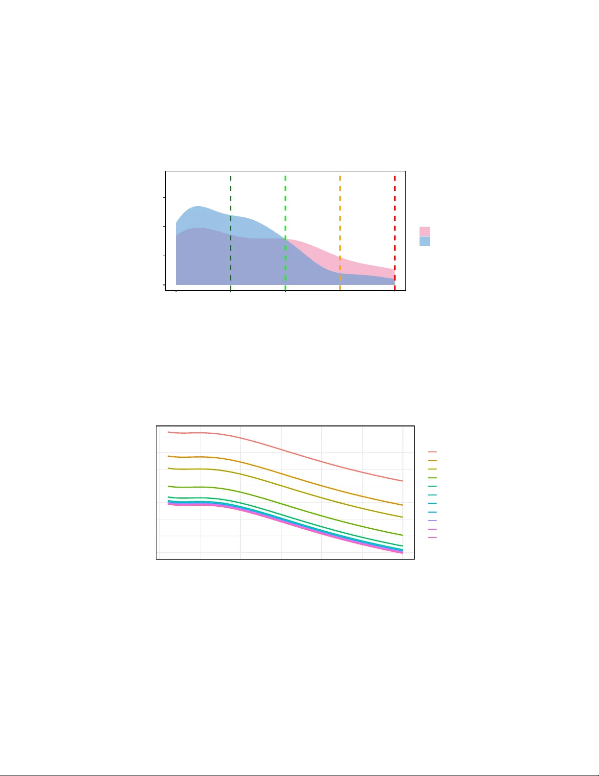
Ba y esian Analysis (TBA) TBA , Num b er TBA, pp. 1 Diﬀerentially p rivate Ba y esian tests Abhisek Chakrab ort y, Saptati Datta Abstract. Diﬀeren tial priv acy has emerged as a signiﬁcan t cornerstone in the realm of scien tiﬁc h yp othesis testing utilizing conﬁden tial data. When data are not conﬁden tial, Ba yesian tests are widely used in rep orting scien tiﬁc discov eries, as they eﬀectiv ely address the key criticisms of p-v alues, namely lack of inter- pretabilit y and inabilit y to quan tify evidence in supp ort of comp eting hypotheses. In this article, we introduce a nov el framework for diﬀeren tially priv ate Bay esian h yp othesis testing, thereby expanding the applicabilit y of Bay esian testing to con- ﬁden tial data. This framew ork naturally arises from a principled data-generativ e mec hanism, ensuring that the resulting inferences retain in terpretability while main taining priv acy . F urther, by focusing on diﬀeren tially priv ate Bay es factors based on test statistics, w e circumv ent the need to mo del the complete data gener- ativ e mechanism and ensure substantial computational beneﬁts. W e also provide a set of suﬃcien t conditions to establish Ba yes factor consistency under the pro- p osed framework. Finally , the utilit y of the prop osed metho dology is show cased via sev eral n umerical experiments. MSC2020 subject classiﬁcations : Primary 60K35, 60K35; secondary 60K35. Keyw o rds: Bay es F actors, Ba y es F actor Consistency, Diﬀeren tial Priv acy, In terpretable ML, Laplace Mec hanism. 1 Intro duction Hyp othesis testing is an indispensable to ol to answ er scientiﬁc questions in the context of clinical trials, bioinformatics, so cial sciences, etc. The data within such domains often in v olves sensitive and priv ate information p ertaining to individuals. Researc hers often b ear legal obligations to safeguard the priv acy of such data. In this context, diﬀerential priv acy ( Dw ork , 2006 ) has emerged as a p opular framework for ensuring priv acy in statistical analyses with conﬁden tial data. Consequen tly , diﬀeren tially priv ate versions of numerous commonly used hypothesis tests hav e b een dev elop ed, although exclusiv ely from a frequentist view p oint. This encompasses priv ate adaptations of test of binomial prop ortions ( A wan and Slavk ović , 2018 ), signiﬁcance in linear regression ( Alabi and V adhan , 2023 ), go o dness of ﬁt ( Kw ak et al. , 2021 ), analysis of v ariance ( Swan b erg et al. , 2019 ), high-dimensional normal means ( Naray anan , 2022 ), to name a few. Diﬀeren tially priv ate versions of common non-parametric tests ( Couc h et al. , 2019 ), p ermutation tests ( Kim and Schrab , 2023 ), etc., hav e emerged as w ell. Another recent line of work proposes to automatically create priv ate v ersions of the existing frequen tist tests in a blac k-b o x arXiv: 2010.00000 ∗ Department of Statistics, T exas A&M University , College Station, TX, USA † Both the authors con tributed equally . ‡ There was no external or internal funding for this project. © TBA In ternational Society for Ba yesian Analysis 2 Diﬀeren tially priv ate Bay esian tests fashion ( Kazan et al. , 2023 ; P eña and Barrien tos , 2023 ), utilizing the subsample-and- aggregate metho d, with the aggregation done by the uniformly most p ow erful binomial test ( A wan and Sla vko vić , 2018 ). In this article, w e intend to complement the existing literature via pro viding a nov el generalised framew ork for diﬀerentially priv ate Bay esian testing. This is crucial since p-v alues obtained from frequentist tests are routinely criticised for it’s lack of trans- parency , inability to quan tify evidence in supp ort of the n ull hypothesis, and inability to measure the imp ortance of a result. Readers may refer to the American Statistical Asso ciation statement on statistical signiﬁcance and p-v alues W asserstein and Lazar ( 2016 ) for further discussions on this. On the other hand, Bay es factors ( Kass and Raftery , 1995 ; Jeﬀreys , 1961 ; Morey and Rouder , 2011 ; Rouder et al. , 2009 ; W agen- mak ers et al. , 2010 ; Johnson et al. , 2023a ) can quantify the relativ e evidence in fa vor of comp eting h yp otheses, eﬀectively addressing the p ersisten t criticisms of p-v alues. This automatically calls for dev elopment of diﬀerentially priv ate Bay es F actors to test the scien tiﬁc hypotheses of interest with conﬁden tiality guarantees. Prior to presen ting the proposed methodology , w e pro vide a concise ov erview of p ertinen t concepts in Bay esian h yp othesis testing and diﬀerential priv acy , laying the groundw ork for subsequen t discussions. 1.1 Ba yesian hyp othesis testing Supp ose w e i n tend to test the n ull h yp othesis H 0 : θ ∈ Θ 0 against the alternativ e h yp othesis H 1 : θ ∈ Θ 1 . The Bay es F actor ( Kass and Raftery , 1995 ; Jeﬀreys , 1961 ; Morey and Rouder , 2011 ; Rouder et al. , 2009 ; W agenmak ers et al. , 2010 ; Johnson et al. , 2023a ) in fav our of the alternativ e h yp othesis H 1 against the null hypothesis H 0 is deﬁned as BF 10 = P ( H 1 | x ) P ( H 0 | x ) = m 1 ( x ) m 0 ( x ) × P ( H 1 ) P ( H 0 ) , (1.1) where P ( H i | x ) is the p osterior probability of H i giv en the data x , P ( H i ) is the prior probabilit y assigned to H i , and M i ( x ) denotes the marginal probabilit y assigned to the data under H i , i = 0 , 1 . The marginal densities are computed via m i ( x ) = Z Θ i π ( x | θ ) π i ( θ ) dθ , where π ( x | θ ) is the data generative mo del given the parameter θ , and π i ( θ ) is the prior density for θ under H i , i = 0 , 1 . Bay es factor eﬀectiv ely addresses the p ersistent criticisms regarding lack of in terpretability of p-v alues ( W asserstein and Lazar , 2016 ) in rep orting outcomes of h yp othesis tests, since it directly quan tiﬁes the relativ e evidence in fav or of the comp eting hypotheses H 0 and H 1 . Noteworth y , the v alue of a Bay es factor dep ends on the choices of π i ( θ ) , i = 0 , 1 , and it is generally diﬃcult to justify an y single default choice. Moreov er, the expression of M i ( x ) , i = 0 , 1 ma y not b e a v ailable in closed form, and require computing a p otentially high-dimensional n umerical integral. Sev eral mo diﬁcations to the existing Bay es factor metho dology are prop osed to impro ve Chakrab ort y and Datta 3 the rep orting of scien tiﬁc ﬁndings. T w o suc h mo diﬁcations of traditional Bay es factors, that will be utilized to construct diﬀerentially priv ate Bay esian tests, are Bay es factors constructed based on common test statistics (BFBOTS) ( Johnson , 2005 ) and Bay es factors rep orted as a function of eﬀect size (BFF s) ( Johnson et al. , 2023b ). W e brieﬂy review b oth the ideas next. 1.2 Ba yes facto r based on test statistics T o circumnavigate the issues with traditional Bay es factors, Johnson ( 2005 ) prop osed to deﬁne Bay es factors based on common test statistics, and put priors directly on the non-cen tralit y parameter of the test statistics to sp ecify the v arious comp eting hypothe- ses. Bay es factors are ﬁrst deﬁned in terms of standard z , t , χ 2 , and F test statistics. The distribution of these test statistics under the null hypothesis is known. Under the alternativ e hypotheses, their asymptotic distributions are common non-central distribu- tions, characterized solely b y scalar-v alued non-centralit y parameters. As a result, the sp eciﬁcation of the prior density under the alternative hypothesis is simpliﬁed, and no prior density is required under the null hypothesis. F or example, supp ose w e observe data X 1 , . . . , X n ∼ N ( µ, σ 2 ) , and wan t to test H 0 : µ = 0 against H 1 : µ  = 0 . In this con text, under H 0 , the t -statistic t = √ n ¯ X ˆ σ follo ws a student’s t n − 1 (0) distribution with degrees of freedom n − 1 , where ¯ X and ˆ σ are the mean and standard deviation of the observ ed data. Under H 1 the t -statistic t = √ n ¯ X ˆ σ follo ws a (non-central) t n − 1 ( δ ) distri- bution with non centralit y parameter δ ≥ 0 and degrees of freedom n − 1 . In other words, the non centralit y parameter δ = 0 under H 0 and δ > 0 under H 1 . So, we can elicit priors directly on the non-cen tralit y parameter δ under H 1 , and conduct a Ba y esian testing. Moreov er, if w e utilise non-lo cal priors ( Johnson and Rossell , 2010a ) on δ under H 1 instead of local priors, not only the expression of the marginal likelihoo ds are often a v ailable in closed form, but also it ensures quic k accumulation of evidence in fav or of b oth true H 0 and true H 1 . Data-driven approaches for the prior hyper-parameter tuning ( Johnson et al. , 2023a ; Datta et al. , 2024 ) were subsequen tly suggested, adding to the ob jectivit y of suc h Bay esian testing metho dology . 1.3 Ba yes facto r functions(BFFs) In Johnson et al. ( 2023b ), the authors deﬁned Bay es factor functions (BFF s) as a map- ping from standardized eﬀect sizes of in terest to corresp onding Bay es factors, or more precisely , as a mapping from prior densities cen tered on the standardized eﬀect sizes of in terest to the corresponding Bay es factors. F or a given v alue of the test statistic, a range of Bay es factors based on the test statistic v alue is calculated b y v arying the prior densities elicited on the non-centralit y parameter that deﬁnes the alternative hypothe- sis. In other w ords, the families of prior densities used to deﬁne these Bay es factors are indexed by the standardized eﬀect size. Through this mapping, BFF s make the relation- ship b etw een Ba y es factors and prior assumptions more transparent by providing a clear in terpretation of Ba y es factors as a function of prior densities used in their formulation. A dditionally , another crucial feature of BFF s relev ant to us is that the BFF s enable the accum ulation of evidence across m ultiple studies examining the same phenomenon. 4 Diﬀeren tially priv ate Bay esian tests T o elucidate the construction of a BFF, let us reconsider a tw o-sided t -test as previ- ously discussed. Let X 1 , . . . , X n b e indep endent and identically distributed as N ( µ, σ 2 ) , where σ 2 is unknown, and deﬁne the test statistic as t = √ n ¯ x/σ . Under this set up, t ∼ t n − 1 ( √ nπ ∗ ) , where π ∗ = µ/σ represents the standardized eﬀect, and λ = √ nπ ∗ is the non-centralit y parameter asso ciated with the test statistic. Under the n ull hypothe- sis, we hav e H 0 : λ = 0 , and no prior sp eciﬁcation on λ is required. Under the alternativ e h yp othesis H 1 : λ  = 0 , we ma y sp ecify a normal-moment prior densit y ( Johnson and Rossell , 2010b ), as follo ws: H 1 : t | λ ∼ t n − 1 ( λ ) , λ ∼ j ( λ | τ 2 ) , where j ( λ | τ 2 ) = λ 2 √ 2 π τ 3 exp  − λ 2 2 τ 2  , λ ∈ R , and τ 2 is a prior h yp er-parameter. The mo de of the prior density j ( λ | τ 2 ) o ccurs at ± √ 2 τ . F or a giv en v alue of standardized eﬀect size π ∗ , if w e set τ 2 = nπ ∗ 2 / 2 , then the mo de of the prior densit y equals √ nπ ∗ . Consequently , the mo de of the prior densit y aligns with the non-centralit y parameter λ of the test statistic. Utilizing this relationship, Bay es F actor F unctions (BFF s) are dev elop ed to asso ciate standardized eﬀect sizes with corresp onding Bay es factors. Sp eciﬁcally , for a giv en standardized eﬀect size, the Ba y es factors are computed using alternative prior densities that are centered on non-cen tralit y parameters aligned with the sp eciﬁed standardized eﬀect size. W e next pro vide a succinct ov erview of relev ant concepts from diﬀerential priv acy literature. 1.4 Diﬀerential privacy Diﬀeren tial priv acy ( Dwork , 2006 ; Baraheem and Y ao , 2022 ) presents a principled frame- w ork for safeguarding sensitive information in conﬁdential data utilized for statistical analyses. It achiev es this by ensuring that the probability of any sp eciﬁc output of the statistical pro cedure is nearly the same, regardless of the data b elonging any one sp eciﬁc individual in the database. In this context, databases that v ary only with resp ect to the data corresp onding to a single individual are termed neighb oring databases. Deﬁnition 1 (Diﬀerential Priv acy , ( Dwork , 2006 )) . A r andomize d algorithm f : D → S is ε -diﬀer ential ly private if for al l p ossible outc omes S ⊆ S and for any two neighb ouring datab ases D , D ′ ∈ D , we have P [ f ( D ) ∈ S ] ≤ e ε P [ f ( D ′ ) ∈ S ] . F urther, the measure of how muc h the mo diﬁcation of a single ro w in a database can inﬂuence the output of a query is referred to as glob al sensitivity . Deﬁnition 2 (Global sensitivit y) . The glob al sensitivity of a function f is GS f = max D , D ′ ∈D | f ( D ) − f ( D ′ ) | , wher e D and D ′ ar e neighb oring datab ases. The privacy budget ε quan tiﬁes the degree of priv acy protection, with smaller v al- ues of ε indicating a stronger priv acy guarantee. In particular, ε -diﬀeren tial priv acy ensures that the priv acy loss is b ounded by ε almost surely , which implies that the Chakrab ort y and Datta 5 ratio of the output probabilities under neighboring datasets is constrained b y e ε for all outcomes. As ε becomes smaller, the priv acy of the mechanism f increases, since the output distributions under neighboring datasets f (D) and f (D ′ ) are forced to b e similar ( Barrien tos et al. , 2019 ). Every diﬀerentially priv ate algorithm achiev es this via incorp o- rating an element of randomness. One of the most widely adopted such technique is the Laplace mec hanism ( Dwork , 2006 ), that inv olves introducing a priv acy noise sampled from Laplace distribution to the result of the query that requires priv acy protection. The scale of the Laplace distribution employ ed to introduce the priv acy noise, is con tin- gen t on b oth the priv acy budget ε and the global sensitivity GS f . Given an y function f , the L aplac e me chanism is deﬁned as ˜ f ( D ) = f ( D ) + η , where η is a priv acy noise dra wn from Laplace (0 , GS f /ε ) , and GS f is the global sensi- tivit y of f . W e now hav e reviewed all the necessary tools to introduce our metho dology . 1.5 Relevant literature There has b een gro wing in terest in developing Ba yesian inferen tial metho ds under the diﬀeren tial priv acy (DP) framew ork. A notable contribution in this area is by Peña and Barrientos ( 2023 ), who prop osed a diﬀerentially priv ate hypothesis test based on a subsample-and-aggregate sc heme. While their metho d primarily aligns with frequentist principles—fo cusing on assessing null hypothesis ﬁt—they also extend it to the Bay esian paradigm by computing p osterior o dds based on the distribution of the test statistics they introduce. How ever, due to the nature of their test statistic, the resulting Bay es factor lacks consistency under the alternative hypothesis. Additionally , the metho d relies on a sub jective prior for the test’s p ow er, rendering the Bay es factor sensitive to this prior sp eciﬁcation. T o address these limitations, P eña and Barrientos ( 2024 ) in tro duced an alternative diﬀerentially priv ate test that uses truncated likelihoo d ratio statistics or truncated Bay es factor, eﬀectively bounding the global sensitivity of the Bay es factor. While this approach improv es priv acy guarantees, it raises interpretabilit y concerns, as the truncation is not deriv ed from the underlying generative mo del. In the context of linear regression, Amitai and Reiter ( 2018 ) prop osed tw o ap- proac hes for Ba yesian inference based on p osterior probabilities of regression co eﬃcients. The ﬁrst approach assumes a normal appro ximation to the p osterior and requires unbi- ased p osterior estimates of the co eﬃcients, making it suitable primarily for large sample sizes. The second approach aggregates p osterior probabilities using Fisher’s metho d and assumes that the resulting statistic follows a χ 2 distribution. This assumption fails under the alternative hypothesis. Moreo v er, their metho d in volv es clipping p osterior probabil- ities at a ﬁxed threshold, which ma y suppress evidence against the null. Imp ortantly , their work do es not fo cus sp eciﬁcally on Ba y esian hypothesis testing. Other notable con tributions include Bernstein and Sheldon ( 2019 ), who prop osed a diﬀeren tially priv ate method for posterior sampling of regression parameters, although their w ork does not directly address hypothesis testing. In parallel, Dimitrakakis et al. ( 2017 ); Heikkilä et al. ( 2019 ); Hu et al. ( 2023 ) dev elop ed v arious techniques for drawing 6 Diﬀeren tially priv ate Bay esian tests p osterior samples under diﬀerential priv acy constraints. These metho ds t ypically rely on the assumption of a b ounded likelihoo d and require a priv acy budget that scales with the num b er of p osterior samples. Consequently , when the priv acy budget is small, suc h approaches may yield unreliable Monte Carlo appro ximations. Dra wing inspiration from these w orks, w e propose an ob jective Bay esian testing pro cedure that is consisten t under the true hypothesis. 1.6 Our contributions The k ey con tributions in the article are three-fold. First, to the b est of our kno wledge, w e introduce the ﬁrst-ever diﬀerentially priv ate ob jective Bay esian testing framework and ensure the consistency of the Ba yes factor under the true mo del. This developmen t is imp ortant in ligh t of the American Statistical Asso ciation’s statement on statistical signiﬁcance and p-v alues ( W asserstein and Lazar , 2016 ), whic h w arns against making scien tiﬁc decisions based solely on p-v alues, due to their lac k of transparency , inability to quantify evidence supp orting the null hypothesis, and failure to measure the practical signiﬁcance of a result. While Ba y es factor-based tests oﬀer a solution to many of the limitations asso ciated with p-v alues, extending these tests to a diﬀeren tially priv ate set- ting—while preserving their inherent interpretabilit y—presents substan tial challenges. T o address this, we integrate widely-used strategies in diﬀerentially priv ate testing, such as sub-sample and aggregate metho ds and truncated test functions, within the prop osed data-generativ e mechanism. This careful in tegration ensures that the resulting Ba y esian testing procedures emerge naturally from the data generation models, main taining the in terpretabilit y of the resulting inferences. Second, we in tro duced diﬀerentially priv ate Bay es factors that rely on widely-used test statistics, extending the w ork of Johnson ( 2005 ) to a priv acy-preserving frame- w ork. In this approac h, w e place priors directly on the non-cen trality parameter of the test statistic and emplo y data-driv en tec hniques for tuning prior h yp erparameters. This strategy eliminates the need to mo del the entire data-generating pro cess and av oids plac- ing priors on p otentially high-dimensional mo del parameters. As a result, the metho d oﬀers signiﬁcant computational adv an tages when calculating marginal likelihoo ds, which t ypically in volv e intractable integrals in fully parametric Bay esian testing frameworks. F urthermore, we establish a set of suﬃcient conditions to ensure the consistency of the Bay es factor ( Chib and Kuﬀner , 2016 ; Chatterjee et al. , 2020 ) within the proposed framew ork. Finally , w e critically lev erage the proposed Ba yes factor based on test statistics framew ork, to oﬀer a general template for constructing size- α diﬀerentially priv ate Ba y esian tests that adhere to a predeﬁned priv acy budget, pro vided the inv estigator has pre-sp eciﬁed the eﬀect size of in terest. Additionally , w e propose n umerical sc hemes for data-driven hyperparameter tuning. Sp eciﬁc examples under particular hypothesis testing scenarios are presen ted. Nevertheless, the applicability of the prop osed sc hemes extends b ey ond the Ba y es factors based on test statistics discussed in this article. In a nutshell, the k ey diﬀerences betw een our con tribution and the existing works of P eña and Barrientos ( 2023 ); P eña and Barrientos ( 2024 ) and Amitai and Reiter ( 2018 ) Chakrab ort y and Datta 7 are as follo ws: 1. W e in tro duce Bay es factors for hypothesis testing within an ob jective Bay esian framew ork, whic h eliminates the dependence on sub jectiv e prior elicitation. This ensures that the resulting Bay es factors are interpretable and mitigates the sensi- tivit y to prior speciﬁcations that is present in the approac hes of P eña and Barri- en tos ( 2023 ). 2. Unlik e Peña and Barrien tos ( 2024 ), our method do es not require an y direct trun- cation scheme to guaran tee the b oundedness of the General Sensitivity Parameter (GSS). This prop erty is inheren tly satisﬁed by our model sp eciﬁcation and prior c hoice. As a result, we retain full interpretabilit y of the Ba yes factor, which may b e compromised in Peña and Barrientos ( 2024 ) due to the non-generativ e trunca- tion required to b ound the GSS. Consequently , the Ba yes factor in their work can b e hard to in terpret. 3. W e ev aluate the Bay es factor ov er a sequence of alternativ e h yp otheses indexed b y the eﬀect size of interest, which introduces additional ﬂexibility . 4. As outlined in our general framework, presented in Section 2 , the prop osed metho d extends well b eyond test statistic-based Bay es factors. W e emphasize Ba yes factors based on test statistics primarily to av oid sub jective priors on n uisance parame- ters. W e use suﬃcient statistics to deﬁne Ba yes factors, thereb y ensuring there is no p otential information loss. How ever, our general framework can encompass a broader class of models. 5. In con trast to Amitai and Reiter ( 2018 ), our primary ob jective is hypothesis test- ing for the purp ose of mo del selection. W e aim to achiev e b oth interpretabilit y and consistency in mo del selection, b oth under the n ull and alternative hypotheses. Rest of the article is organized as follo ws. Section 2 introduces the prop osed frame- w ork for diﬀeren tially priv ate Ba yesian testing in complete generalit y , and presen ts the k ey features of the metho dology . In Section 3 , w e in tro duce diﬀeren tially priv ate Ba y esian tests based on common test statistics, discuss their asymptotic properties under v arious common hypothesis testing problems and discuss sc hemes for the hyper- parameter tuning under the prop osed technology . In Section 4 , w e study the numerical eﬃcacy of the prop osed technology in diﬀerent hypothesis testing problems with prac- tical utility . Finally , w e conclude with a discussion. 2 General framew o rk In this section, the ob jectiv e is to lay do wn a hierarchical mo del equipp ed with care- fully c hosen priors on the parameter of in terest to sp ecify comp eting hypotheses, whic h naturally gives rise to the prop osed diﬀerentially priv ate Bay esian tests. Notably , this attribute remains elusive in the existing literature and that hinders the interpretabilit y of the resulting inference. In particular, man y existing diﬀeren tially priv ate frequentist 8 Diﬀeren tially priv ate Bay esian tests testing pro cedures ( Peña and Barrientos , 2023 ; Kazan et al. , 2023 ) rely on an ad-ho c sampling and aggregation scheme coupled with a test statistic truncation step, to formu- late the desired tests. Despite the empirical success of such methods, a signiﬁcant deﬁ- ciency stems from the lack of a principled probabilistic in terpretation, i.e, suc h metho ds do es not enable us to quan tify evidence in fav or of the n ull and alternative h yp otheses. W e sp eciﬁcally tac kle this issue in the subsequen t discussions. 2.1 Hiera rchical mo del and prio r sp eciﬁcation F or a p ositive in teger t , denote [ t ] : = { 1 , . . . , t } . Supp ose we observ e data x = ( x 1 , . . . , x n ) ′ from a probability distribution having densit y π ( · | θ ) , θ ∈ Θ . W e then randomly divide the data into M n partitions x ( i ) , i ∈ [ M n ] . W e can assume that the data in eac h of the M n partitions arise from x ( i ) ∼ n i Y j =1 π ( x ( i ) j | θ ( i ) ) , indep enden tly for i ∈ [ M n ] , (2.1) suc h that P M n i =1 n i = n . The ab ov e data generating sc heme comes in handy to formalize the sample and aggr e gate scheme under the prop osed setup. In priv acy-preserving in- ference, this subsample–and–aggregate structure pla ys a crucial role in controlling the global sensitivity of the resulting quantit y of interest, e.g, test statistic, Bay es factor. By splitting the dataset in to m ultiple partitions, computing intermediate quan tities within eac h subset, and then aggregating these results, one can approximate the full-sample quan tit y of in terest. This construction provides the foundation for the prop osed diﬀer- en tially priv ate Ba yes factor, as it allo ws the priv acy noise to scale with the sensitivity of the partition-lev el statistics rather than the en tire dataset. Next, we p osit the priors on the parameter of in terest θ under the comp eting hy- p otheses. T o that end, w e assume that θ ( i ) | τ 0 ,i , τ 1 ,i ∼ (1 − ω n ) π 0 ( θ ( i ) | τ 2 0 ,i ) + ω n π 1 ( θ ( i ) | τ 2 1 ,i ) under H 0 , θ ( i ) | τ 0 ,i , τ 1 ,i ∼ ω n π 0 ( θ ( i ) | τ 2 0 ,i ) + (1 − ω n ) π 1 ( θ ( i ) | τ 2 1 ,i ) under H 1 , (2.2) indep enden tly for i ∈ [ M n ] , where { π i ( · ) , i = 0 , 1 } are the prior probability distribu- tions, ( τ 0 ,i , τ 1 ,i ) are prior hyper-parameters, and ω n ∈ (0 , 1 2 ) is a hyper-parameter that ensures that the Ba y es factor for testing H 0 against H 1 is b ounded. W e will later on sho w that ω n dep ends on the sample size n and hence ﬁnd it necessary to index it with n . If the Ba yes factor for testing H 0 against H 1 w ere to be un b ounded, the global sensitivit y parameter of the Bay es factor b ecomes un b ounded to o. An immediate ﬁx against it w ould inv olve truncating the log Ba y es factor beyond an interv al of the form [ − a n , a n ] , a n > 0 or more generally [ L n , U n ] with L n < U n , akin to the approach in P eña and Barrientos (2024). If one were to adopt the framework of Peña and Barri- en tos (2024), impose non-lo cal priors on the parameters of interest, and implement an ob jectiv e Bay esian hyper-parameter tuning strategy similar to that used in the presen t w ork, one w ould obtain a Bay es factor with op erating c haracteristics comparable to the diﬀeren tially priv ate Bay es factor developed here. How ever, suc h a construction would Chakrab ort y and Datta 9 lac k the interpretabilit y aﬀorded by our formulation, which arises from a hierarchical mo del with carefully sp eciﬁed priors that directly enco de the comp eting hypotheses and thereb y yield the prop osed diﬀeren tially priv ate Ba yesian tests in a principled manner. Up on closer lo ok, truncating the log Ba yes factor in principle means that the maximum evidence that we can obtain in fa vor of H 0 (or H 1 ) against H 1 (or H 0 ) is b ounded from ab o v e – we precisely imp ose this constraint a-priori via the hierarchical sp eciﬁcation (2.2), thereby eliminating the need for truncation/p ost-pro cessing. F or each partition x ( i ) , i ∈ [ M n ] , we record the notations for the in tegrals m k ( x ( i ) | τ 2 k,i ) = Z Θ  n j Y j =1 π ( x ( i ) j | θ ( i ) )  π k ( θ ( i ) | τ 2 k,i ) dθ ( i ) , k = 0 , 1 . Giv en ω n , τ 0 ,i , τ 1 ,i , and assuming indep endence, the marginal m k ( x | τ 2 k,i ) is the pro duct of the marginals across each partition, m k ( x ( i ) | τ 2 k,i , ω n ) . Consequently , since the Ba y es factor is the ratio of these marginal densities with equal prior probabilities on the h yp otheses, it b ecomes the pro duct of the individual Ba yes factors for eac h partition. Aggregation of evidence across partition is further detailed in Section 2.2. In summary , the mixture priors on { θ ( i ) , i ∈ [ M n ] } under the comp eting hypotheses are instrumental in formalizing the trunc ation scheme necessary to ensure that the global sensitivit y parameter of the priv acy mechanism is b ounded, while preserving the interpretabilit y of the resulting Bay es factors. One ma y criticize the app earance of the parameter ω n in our formulation. T o that end, we carefully introduce an asymptotic regime to analyze the prop osed metho dology , so that the eﬀect of ω n w ashes aw ay as the sample size div erges to ∞ . The mo del and prior sp eciﬁed in equations ( 2.1 )-( 2.2 ), together with the assumption that P ( H 0 ) = P ( H 1 ) = 0 . 5 , (2.3) apriori, completely describ e our generative mo del of interest. 2.2 Prop erties W e note that for eac h partition x ( i ) , i ∈ [ M n ] , the quan tit y m k ( x ( i ) | τ 2 k,i ) , k = 0 , 1 , can b e interpreted as the marginal likelihoo d of the data partition x ( i ) under the hypothesis H k when ω n = 0 . Under this set up, as we eluded to earlier, the Ba yes factor for testing H 0 against H 1 can b e un b ounded, and consequen tly the global sensitivity parameter of the priv acy mechanism is unbounded to o. This renders the dev elopment of diﬀerentially priv ate Bay esian tests non-trivial, and throughout the article w e shall assume that the hyper-parameter ω n > 0 . Under the alternative hypothesis H 1 in ( 2.1 )-( 2.3 ), the marginal distribution of the data partition x ( i ) is expressed as m t 1 ( x ( i ) | τ 2 0 ,i , τ 2 1 ,i , ω n ) = ω n m 0 ( x ( i ) | τ 2 0 ,i ) + (1 − ω n ) m 1 ( x ( i ) | τ 2 1 ,i ) , i ∈ [ M n ]; and under the n ull h yp othesis H 0 , it is giv en b y: m t 0 ( x ( i ) | τ 2 0 ,i , τ 2 1 ,i , ω n ) = (1 − ω n ) m 0 ( x ( i ) | τ 2 0 ,i ) + ω n m 1 ( x ( i ) | τ 2 1 ,i ) , i ∈ [ M n ] . 10 Diﬀeren tially priv ate Bay esian tests Consequen tly , in light of the data partition x ( i ) , the Bay es factor against the null hy- p othesis H 0 is expressed as BF t 10 ( x ( i ) | τ 2 0 ,i , τ 2 1 ,i , ω n ) = ω n + (1 − ω n )  m 1 ( x ( i ) | τ 2 1 ,i ) / m 0 ( x ( i ) | τ 2 0 ,i )  (1 − ω n ) + ω n  m 1 ( x ( i ) | τ 2 1 ,i ) / m 0 ( x ( i ) | τ 2 0 ,i )  , i ∈ [ M n ] . (2.4) W e pro ceed b y listing out the key prop erties of the Bay es factor against the n ull hy- p othesis BF t 10 ( x ( i ) | τ 2 0 ,i , τ 2 1 ,i , ω n ) for the data partition x ( i ) . Lemma 2.1. F or ω n ∈ (0 , 1 / 2) , BF t 10 ( x ( i ) | τ 2 0 ,i , τ 2 1 ,i , ω n ) is b ounde d b etwe en [ ω n 1 − ω n , 1 − ω n ω n ] . Lemma 2.2. Under ( 2.1 ) - ( 2.3 ) , the Bayes F actor against the nul l hyp othesis H 0 c om- bine d acr oss al l the p artitions x ( i ) , i ∈ [ M n ] is expr esse d as BF t 10 ( x | τ 2 0 ,i , τ 2 1 ,i , ω n ) = M n Y i =1 BF t 10 ( x ( i ) | τ 2 0 ,i , τ 2 1 ,i , ω n ) . Corollary 2.2.1. L emma 2.1 to gether with L emma 2.2 implies that, the c ombine d Bayes F actor against the nul l hyp othesis H 0 acr oss al l the p artitions x ( i ) , i ∈ [ M n ] , BF t 10 ( x | τ 2 0 ,i , τ 2 1 ,i , ω n ) is b ounde d b etwe en  ω n 1 − ω n  M n and  1 − ω n ω n  M n for ω n ∈ (0 , 1 / 2) . In the sequel, w e construct diﬀeren tial priv ate Ba yesian tests based on the ran- domised mechanism, denoted by f , that map a data set x to the av erage log Bay es factor f 10 ( x ) = 1 M n log BF t 10 ( x | τ 2 0 ,i , τ 2 1 ,i , ω n ) = 1 M n M n X i =1 log BF t 10 ( x ( i ) | τ 2 0 ,i , τ 2 1 ,i , ω n ) . (2.5) W e take refuge to common diﬀeren tial priv acy mec hanism of adding calibrated priv acy noise to the randomised mechanism f to ensure diﬀerential priv acy of the inferential pro cedure. F or every data set x , since the log Bay es factor in each of the partitions log BF t 10 ( x ( i ) | τ 2 0 ,i , τ 2 1 ,i , ω n ) is b ounded b etw een [ − a n , a n ] with a n = − log ( ω n / 1 − ω n ) , the global sensitivity of log BF t 10 ( x ( i ) | τ 2 0 ,i , τ 2 1 ,i , ω n ) is 2 a n . Consequen tly , the global sensitivit y of GS f of the log Ba yes factor a v eraged o ver the partitions, i.e of f , is (2 a n / M n ) . W e now hav e all the necessary ingredien ts to introduce our priv acy preserving mec hanism. T o that end, let D denote the collection of all p ossible data sets. W e consider a random mechanism H : D → R expressed as H 10 ( x ) = f 10 ( x ) + η , x ∈ D , (2.6) where η is a Laplace (0 , GS f /ε ) distributed priv acy noise. A test based on H 10 ( x ) is then obtained as ϕ ( x ) = ( 1 if H 10 ( x ) ≥ γ α,ε ( n ) , 0 otherwise , (2.7) Chakrab ort y and Datta 11 for some cut-oﬀ γ α,ε ( n ) , dep ending on the sample size n and size α of the test. Here, ϕ ( x ) = 1 signiﬁes rejection of H 0 / acceptance of H 1 , and if ϕ ( s ) = 0 , accept H 0 . Theorem 2.3. The function ϕ ( x ) for testing H 0 against H 1 , as describ e d in ( 2.5 ) - ( 2.7 ) , is ε -diﬀer ential ly private. Pr o of. The global sensitivity GS f of f ( x ) is 2 a n M n . Then, deﬁning H ( x ) = f ( x ) + η , where η follows Laplace (0 , GS f /ε ) completes the proof, b y deﬁnition. Next, w e dev elop diﬀerentially priv ate Bay es factors based on widely-used test statis- tics, and crucially lev erage the prop osed framework to provide a systematic approach for selecting γ α,ε ( n ) that maintains a predetermined priv acy budget, assuming the in- v estigator sp eciﬁes the eﬀect size of interest in adv ance. 3 Diﬀerentially p rivate Ba y es factors based on test statistics The general framework presented in Section 2 can b e employ ed to devise fully para- metric Ba y esian tests that preserv es diﬀerential priv acy . How ever, given the limitations of Ba yes factors derived from fully parametric mo dels, as outlined in the in tro duction, and in order to ensure straightforw ard preserv ation of ( ε, 0) -diﬀerential priv acy in the prop osed mechanism, we instead dev elop diﬀerentially priv ate Bay es factors based on test statistics. On top of computational simplicity and ob jectivit y , a major b eneﬁt of represen ting Bay es factors in terms of test statistics that is crucial for us is that they can b e formulated as a function of the standardized eﬀect size ( Johnson et al. , 2023b ; Datta et al. , 2024 ), if we sp ecify the comp eting h yp otheses in ( 2.2 ) using a mixture of a spik e at 0 and an appropriately chosen ﬁrst order non-local prior ( Johnson and Rossell , 2010b ; Johnson et al. , 2023b ) on the non-centralit y parameter of the appropriate test statistic. Moreo ver, suc h non-lo cal priors contain a single scale parameter that con trol the mo de of the prior densities that in turn can b e utilized to deﬁne the null and alter- nativ e h yp otheses. By determining the prior mo de using a function of the standardized eﬀect size (analogous to BFF s.), we can derive Bay es factors for a sequence of n ull and alternativ e hypothesis. In particular, the hyper parameter τ 2 1 ,i in ( 2.2 ) can b e ob jectively determined based on the standardized eﬀect size of interest to express our Bay es factors as functions of the sequence of n ull and alternativ es. This enables us to determine a priv atized cut-oﬀ γ α,ε ( n ) that v aries for each sequence of null and alternatives, while adhering to pre-sp eciﬁed priv acy budget. Bey ond aiding the computation of the cut-oﬀ v alue γ α,ε ( n ) , suc h that ( ϵ, 0) -diﬀeren tial priv acy is ensured, the choice of priors throughout the rest of the article is further guided b y tw o other considerations. First, the carefully chosen non-lo cal priors ensure that b oth the marginal likelihoo ds under the tw o comp eting hypotheses of interest are av ailable in closed form. This eliminates the computational expenses asso ciated with the n umerical ev aluation of the otherwise intractable m ultiple integrals. Secondly , and perhaps more 12 Diﬀeren tially priv ate Bay esian tests imp ortan t, the prior speciﬁcation ensures rapid accumulation of evidence in fa vor of the true hypothesis. W e shall no w formally introduce the diﬀerentially priv ate Ba yes factor based on test statistics. W e note that, the partition sp eciﬁc log Bay es factor based on test statistic log BF t 10 ( x ( i ) | τ 2 0 ,i , τ 2 1 ,i , ω n ) , as shown later in Section 3.3 , dep ends on x ( i ) only through the partition sp eciﬁc test statistic, denoted by s ( i ) , i ∈ [ M n ] . T o mak e it explicit, we use the notation log BF t stat , 10 ( s ( i ) | τ 2 0 ,i , τ 2 1 ,i , ω n ) instead of log BF t 10 ( x ( i ) | τ 2 0 ,i , τ 2 1 ,i , ω n ) in the rest of the section. Similarly , we shall use f stat , 10 ( s ) and H stat , 10 ( s ) to denote the non-priv atized and priv atized av erage log Bay es factors, instead of f 10 ( x ) and H 10 ( x ) , resp ectiv ely , where s = ( s (1) , . . . , s ( M n ) ) T . With that, the Ba yesian test function based on test statistic H stat , 10 ( s ) is expressed as H stat , 10 ( s ) = f stat , 10 ( s ) + η , s ∈ D , (3.1) where η is a Laplace (0 , GS f /ε ) distributed priv acy noise. Similar to the general frame- w ork, a test based on H stat , 10 ( s ) is then obtained as ϕ ( s ) = ( 1 if H stat , 10 ( s ) ≥ γ α,ε ( n ) , 0 otherwise , (3.2) for some cut-oﬀ γ α,ε ( n ) , dep ending on the sample size n and size α of the test. Here, ϕ ( s ) = 1 signiﬁes rejection of H 0 / acceptance of H 1 , and if ϕ ( s ) = 0 , accept H 0 . Next, giv en the sample size n , priv acy mec hanism, the user deﬁned parameters ( ε, a n , M n ) , and the size α of the test, we determine the cut oﬀ γ α,ε ( n ) by satisfying the size c onstr aint Ξ 0 ( M n | ε, α, n ) = E  ϕ ( s ) | H 0 ] = P H 0  H ( s ) ≥ γ α,ε ( n )  = α. (3.3) Exact calculation of the cut oﬀ γ α,ε ( n ) may not b e amenable under certain cases. How- ev er, we can alw ays obtain γ α,ε ( n ) via a Mon te Carlo sim ulation. W e present the for- malized algorithm to determine the cutoﬀ v alue γ α,ε ( n ) in Algorithm 1 . Determination of the cut oﬀ is further demonstrated in the experiment section. 3.1 Selection of size α cut-oﬀ γ α,ε ( n ) Giv en the priv atized av erage logarithm of Ba yes factor based on test statistic H stat , 10 as deﬁned in ( 3.2 ), our goal in Algorithm 1 is to compute the asso ciated size α cut-oﬀ γ α,ε via a Monte Carlo scheme. Such Monte Carlo approaches are ubiquitous in literature in ﬁnding cut-oﬀs of test functions; see Barrien tos et al. ( 2019 ) for an example in context of diﬀerentially priv ate frequen tist tests. The inputs of the Algorithm 1 are (a) the priv acy budget ε , (b) the n um b er of partitions M n , and truncation level of the partition sp eciﬁc log Bay es factors a n , (c) the standardised eﬀect size of in terest π ∗ , and ﬁnally (d) the n umber of iterations in the Mon te-Carlo simulation N . T o ﬁnd the cut-oﬀ γ α,ε ( n ) , we note that the partition sp eciﬁc Chakrab ort y and Datta 13 common test statistic s ( i ) follo ws a non-central distribution, denoted by S ν i ( λ ( i ) ) , under the null hypothesis in (2.1)-(2.2), where λ ( i ) ∼ (1 − ω n ) δ 0 + ω n π 1 ( λ ( i ) | τ 2 i ) and ν i is a constan t completely determined by the size of the i -th partition of the data. With this insight, at the iteration k ∈ { 1 , . . . , N } of the Monte Carlo sc heme, w e ﬁrst indep enden tly dra w the non-centralit y parameter λ ( i ) from a prior distribution with densit y (1 − ω n ) δ 0 + ω n π 1 ( λ ( i ) | τ 2 i ) and pseudo test statistics s ( i ) k from a non-central distribution S ν i ( λ ( i ) ) , i ∈ [ M n ] . Crucially , the prior hyper-parameter τ 2 i is completely determined by the eﬀect size of interest π ⋆ and size of the i -th partition n i . F or example, for a t -test, we draw the pseudo test statistic s ( i ) k ≡ t ( i ) k from non-cen tral t | n i |− 1 ( λ ( i ) ) distributions with non-cen tralit y parameter λ ( i ) , where λ ( i ) ∼ (1 − ω n ) δ 0 + ω n J ( τ 2 i ) , τ i = √ n i π ⋆ , where J ( τ 2 i ) denotes a normal moment density of order 1, the form of whic h is given by , J ( x | τ 2 ) = x 2 √ 2 π τ 3 exp  − x 2 2 τ 2  , x ∈ R . (3.4) The normal moment prior Johnson and Rossell (2010b); Johnson et al. (2023b) has t w o key features that make it particularly well-suited for Bay esian hypothesis testing. First, it is a nonlo cal prior, meaning it assigns zero probabilit y densit y at the null v alue (t ypically zero). This prop ert y enforces a clear separation b etw een the null and alternativ e h yp otheses by p enalizing parameter v alues close to the null, thereby re- ducing false p ositives and increasing the evidence in fav or of the null when it is true. Second, the normal moment prior improv es mo del selection consistency , esp ecially in high-dimensional or sparse settings. Its structure ensures that, as sample size increases, the Bay es factor reliably fav ors the true mo del—whether it corresp onds to the null or the alternative—leading to more robust and interpretable inference. F or a χ 2 -test, we draw the test statistic s ( i ) k ≡ h ( i ) from a non-central χ 2 ν ( λ ( i ) ) , where λ ( i ) ∼ (1 − ω n ) δ 0 + ω n G (( k / 2) + 1 , 1 / 2 τ 2 i ) , τ 2 i = n i π ⋆ ′ π ⋆ 2 , where G( a, b ) denotes a gamma density with shape parameter a n and rate parameter b . F or an F -test, we draw the test statistic f ( i ) from a non-central F p,n i − p ( λ ( i ) ) for a p ≥ 1 . Then, based on s k = ( s (1) k , . . . , s ( M n ) k ) T , w e calculate the pseudo non-priv ate truncated log Bay es factor f stat , 10 ( s k ) via Equation ( 2.5 ). Then, a priv acy noise η generated from Laplace (0 , 2 a n /εM n ) is added to f stat , 10 ( s k ) to calculate the pseudo priv ate truncated log Bay es factor H stat , 10 ( s k ) via Equation ( 3.1 ). In step (3), w e set the size α cut-oﬀ γ α,ε ( n ) to the 100(1 − α )% quan tile the { H stat , 10 ( s k ) , k ∈ [ N ] } v alues. It is important to note that we are sampling the test statistics from their conditional distributions, S ν ( λ ) , under the n ull hypothesis, where the mode of the slab part of the prior is set by the standardized eﬀect size π ⋆ . In this process, we are not sampling pseudo data, but 14 Diﬀeren tially priv ate Bay esian tests solely the test statistics which only dep end on the partition sp eciﬁc sample size and the standardized eﬀect size of in terest. This ensures the preserv ation of diﬀerential priv acy of the prop osed mec hanism. W e note that for a broad class of mo dels, a suﬃcien t test statistic with a tractable n ull distribution may not exist, even though the full data-generating distribution under b oth the n ull and alternative h yp otheses is known. In such settings, the general frame- w ork describ ed in Section 2 can b e applied directly to the full dataset, without reduction to a test statistic. An explicit algorithm for computing the corresponding Bay es factor cutoﬀ in this full-data setting is provided in Section 2 of the supplemen tary material. Algorithm 1 (Ba yes factor cut-oﬀ) 1: Input. (i) The num b er of partitions M n , (ii) the truncation lev el a n of the partition sp eciﬁc log Ba yes factors, (iii) priv acy parameter ε , (iv) N : The total num b er of the Mon te-Carlo simulations N to estimate the size α cut-oﬀ γ α,ε ( n ) , (v) Standardized eﬀect size of in terest π ⋆ ∈ (0 , 1) . 2: for Standardized eﬀect size of interest π ⋆ do 3: for k = 1 to N do (i) Compute of τ 2 i , i = 1 , 2 , . . . , M n in terms of π ⋆ for each of the M n partitions of the data. F or example, for a z or t test τ 2 i = n i π ⋆ ′ π ⋆ 2 for the i -th partition. 1 (ii) Draw indep endent samples of the non-cen trality parameter, λ ( i ) ∼ (1 − ω n ) δ 0 + ω n π 1 ( λ ( i ) | τ 2 i ) , where π 1 ( λ ( i ) | τ 2 i ) is a non-lo cal moment prior distribution, i ∈ [ M n ] . The prior h yp er-parameter τ 2 i is completely determined by standardized eﬀect size of in terest π ⋆ and the size of the i -th partition n i . (ii) Draw test statistics s ( i ) k from S ν i ( λ ( i ) ) indep enden tly for i ∈ [ M n ] . (iii) Compute BF t stat , 10 ( s ( i ) k | τ 2 i , ω n ) for i ∈ [ M n ] . (iv) Compute f stat , 10 ( s k ) = 1 M n M n X i =1 log BF t stat , 10 ( s ( i ) k | τ 2 i , ω n ) . (v) Generate η from Laplace (0 , 2 a n εM n ) . (vi) Compute H stat , 10 ( s k ) = f stat , 10 ( s k ) + η . 4: end for 5: Output. Compute the size α cut-oﬀ γ α,ε ( n ) , suc h that 100(1 − α )% of the { H stat , 10 ( s 1 ) , . . . , H stat , 10 ( s N ) } v alues are greater than γ α,ε ( n ) . 6: end for 1 Choice of τ 2 i for v arious tests( z, t, χ 2 and F ) can b e found in T able 1 of Johnson et al. ( 2023b ). Chakrab ort y and Datta 15 3.2 Hyp erpa rameter tuning F or the use of diﬀerentially priv ate Ba yesian tests, the concerned parties initially estab- lish the desired priv acy level ε . F ollo wing this determination, we need to select appro- priate v alues for the parameters M n , given a n = − log( ω n / 1 − ω n ) = k n β with ﬁxed 0 < β < 1 , 0 < k ≤ 1 . This iterative pro cess will allow us to exp eriment with div erse v alues of M n , thereb y striking a n uanced balance betw een attaining the desired priv acy lev el and asymptotic b eha vior of the Bay es factors. In this article, we consider the case where we do not hav e the autonom y to select sp eciﬁc v alue of ε , but possess the dis- cretion to choose M n . Analysts, endow ed with the autonomy of choosing the priv acy budget ε , ma y iteratively emplo y the describ ed metho dology , for v arying the v alues of ε . Giv en the sample size n , a priv acy mechanism, a priv acy budget ε , standardized eﬀect size of interest π ⋆ and the size α , we determine the Bay es factor cut oﬀ γ α,ε ( n ) using ( 3.3 ) via a Monte Carlo simulation, for v arying v alues of M n giv en a n . Now, let M denote the space all possibles pairs M n under consideration. W e op erate under the regime that M n = ζ n , 0 < ζ ≤ 1 given a n = k n β . The constraints 0 < β < 1 and 0 < k ≤ 1 ensure that the GS f decreases as the sample size increases. The order assumption on a n , or equiv alently ω n , enables us to dictate the rate at which the hypotheses speciﬁed in Theorems 3.1 - 3.2 (Theorems 3.3 and 3.4 of the Supplementary Material) approach the usual/ non-priv atized n ull hypotheses signiﬁcance testing framework . This, in turn, enables us to dictate the conv ergence rate of the priv atized Bay es factor. Sp eciﬁcally , slo w er the order of a n , low er w ould b e the rate of con v ergence. Refer to Corrollary 3.2.2 and Theorem 3.3 for details. The optimal c hoices M n is obtained via maximising p ower of the test arg max M n ∈M Ξ 1 ( M n | ε, α, n ) where Ξ 1 ( M n | ε, α, n ) = E  ϕ ( s ) | H 1 ] = P H 1  H ( s ) ≥ γ α,ε ( n )  . The n umerical strategy for the h yp er parameter tuning in further demonstrated in Section 4 via examples. 3.3 Ba yes facto rs based on test statistics and convergence rates of Ba yes facto rs In this section, we present the closed form expressions for diﬀerentially priv ate Bay es factors based on common t , χ 2 and F test statistics. F urther, we study the asymptotic prop erties of the prop osed Ba yes factors, adopting the popular notion of Conventional Bayes factor c onsistency ( Chib and Kuﬀner , 2016 ; Chatterjee et al. , 2020 ). Such asymp- totic prop erties must b e satisﬁed to ensure that, as the sample size increases, the correct mo del has a faster rate of p osterior con traction as a function of sample size in compari- son to an incorrect mo del/complex mo del. Results on consistency of Bay es factors based on test statistics ( Johnson , 2008 ; Datta et al. , 2024 ) is not particularly new. How ev er, the introduction of diﬀerential priv acy to this framew ork in tro duces unique challenges. 16 Diﬀeren tially priv ate Bay esian tests T o ensure the conv ergence of the priv atized Ba yes factors, it is essen tial to incorp orate additional meaningful assumptions. This includes considerations ab out the distribution of test statistics under the comp eting h yp otheses ( 2.2 ), order of the truncation param- eter a n (or equiv alently ω n ) and n um b er of data partitions M n relativ e to the sample size, and the c haracteristics of the global sensitivity parameter. Deﬁnition 3 (Conv entional Ba y es factor consistency ( Chib and Kuﬀner , 2016 )) . F or two c omp eting mo dels M l and M k , the Bayes factor for c omp aring mo dels M k and M l , denote d as BF kl = m ( x | M k ) m ( x | M l ) , is c onsistent if (i) BF kl p − → 0 when M l c ontains the true mo del, and (ii) BF kl p − → ∞ when M k c ontains the true mo del, wher e x is the data. Before w e proceed, a few notations are in order. The conﬂuen t h yp er-geometric function of order ( m, n ) ( Abramowitz , 1974 ) is denoted b y m F n ( a, b ; z ) . The Dirac’s delta maesure at 0 is denoted by δ 0 . F urther, N ( a, b ) denotes normal distribution with a mean of a n and v ariance b , T n ( θ ) denotes the t-distribution with degrees of freedom ν and non-centralit y parameter θ , χ 2 n ( θ ) denotes the chi-squared distribution with degrees of freedom ν and non-cen trality parameter θ , F k,m ( θ ) denotes the F-distribution with degrees of freedom ( k , m ) and non-centralit y parameter θ , G ( α, θ ) denotes a gamma distribution with a shape parameter α and a rate parameter θ , and J ( τ 2 ) represen ts a normal-momen t density of order 1 ( Johnson and Rossell , 2010b ). T o guarantee consistency of the Ba yes factors, w e op erate under the asymptotic regime where the num b er of partitions satisﬁes M n = ζ n , for some constan t 0 < ζ ≤ 1 , and the truncation parameter is c hosen as a n = kn β , with 0 < β < 1 and 0 < k ≤ 1 . These assumptions apply uniformly across all tests considered. They arise from the selection of the truncation parameter a n = − log ( ω n / 1 − ω n ) . Recall that, we divide n observ ations in to M n partitions. This asymptotic scaling ensures that the generalized sensitivit y GS f v anishes as n → ∞ , while preserving the rapid conv ergence b ehavior of the priv atized Ba yes factor. W e shall put this statemen t in concrete terms in Theorem 3.3. The generalized sensitivity GS f measures the maximum change in the priv atized statistic when a single observ ation is altered. In the prop osed construction, the test statistic is computed ov er M n = ζ n equally sized partitions, each containing approxi- mately n/ M n = 1 /ζ observ ations. As the total sample size n increases, the contribution of any single observ ation to the aggregated (sample–aggregate) statistic is therefore diluted at rate 1 /n . Consequen tly , the inﬂuence of an individual data p oint on the pri- v atized Bay es factor naturally diminishes as n gro ws. More formally , if the truncation parameter is chosen as a n = k n β with 0 < β < 1 , then the sensitivity of the truncated log Bay es factor satisﬁes GS f = O  a n n  = O  n β − 1  , whic h conv erges to zero for any β < 1 . This falls under the standard “v anishing- sensitivit y” asymptotic regime in diﬀerential priv acy , where the priv acy cost p er individ- ual decreases as the sample size gro ws while the statistical pow er of the test con tinues Chakrab ort y and Datta 17 to impro ve. This assumption is not only mathematically conv enient but also concep- tually aligned with population-level inference, in which the priv acy burden p er sub ject should shrink as more data accumulate. Similar v anishing-sensitivity regimes hav e b een emplo y ed in recen t w ork on diﬀerentially priv ate h yp othesis testing. With these notations, the Bay es F actors based on common test statistics for each partition x ( i ) , i ∈ [ M n ] of the observ ed dataset are presen ted in Theorems 3.1 , 3.2 , and Theorems 3.3, 3.4 of the Supplementary Material, in a manner consistent with the dev elopmen ts of Johnson (2005); Johnson and Rossell (2010b); Johnson et al. (2023b) . Theorem 3.1. ( Two-side d z -test ) Supp ose the gener ative mo del for the test statistic z under H 0 and H 1 ar e H 0 : z | λ ∼ N ( λ, 1) , λ | τ 2 ∼ (1 − ω n ) δ 0 + ω n J ( τ 2 ) H 1 : z | λ ∼ N ( λ, 1) , λ | τ 2 ∼ ω n δ 0 + (1 − ω n ) J ( τ 2 ) , τ > 0 , r esp e ctively. Then, the Bayes factor in favor of the H 1 is of the form BF t 10 ( z | τ 2 , ω n ) = ω n +(1 − ω n ) R (1 − ω n )+ ω n R , wher e R = m 1 ( z | τ 2 ) /m 0 ( z ) = (1 + τ 2 ) − 3 2 1 F 1 (3 / 2 , 1 / 2; τ 2 z 2 / 2(1 + τ 2 )) . Pr o of is deferr e d to the supplementary material. Corollary 3.1.1. Under the set up in The or em 3.1 , we further assume that (i) n mo d M n = 0 and the p artition sp e ciﬁc sample sizes satisfy n i = n/ M n ∀ i ∈ [ M n ] . (ii) the test statis- tic z ( i ) ∼ N ( η √ n i , 1) , for some η ; (iii) the hyp er-p ar ameter τ 2 i = κn i , for some κ > 0 ; (iv) log ((1 − ω n ) /ω n ) = kn β , 0 < β < 1 , 0 < k ≤ 1 . (v) M n = ζ n , 0 < ζ ≤ 1 . Then, under H 0 , Q M n i =1 BF t 10 ( z ( i ) | τ 2 i , ω n ) = O p ( c − n ) , wher e c is a p ositive c onstant. Similarly, under H 1 , Q M n i =1 BF t 01 ( z ( i ) | τ 2 i , ω n ) = O p ( c − n ) . This demonstr ates that the c ombine d Bayes factor, obtaine d fr om the p artition sp e ciﬁc Bayes factors in The or em 3.1 , is c on- sistent under b oth H 0 and H 1 . Pr o of is deferr e d to the supplementary material. Assumption (i) could b e relaxed by permitting n i to increase linearly with n . This assumption is made primarily for clarity and ease of explanation. The justiﬁcation for assumption (ii) is pro vided by the order of commonly utilized z statistics under H 1 . F or instance, consider the test means of an univ ariate normal population N ( µ, 1) . The test statistic of in terest z = √ n ¯ X satisﬁes the assumption, with ¯ X and n being resp ectively the mean and num b er of observ ations collected from the p opulation. Assumption (iii) stems from the selection of τ i = √ n i π ∗ , where π ∗ represen ts the standardized eﬀect size for one-sample z tests. The c hoice of the scale parameter τ 2 i in terms of the sample size and π ∗ for v arious linear tests are listed in T able 1 of Johnson et al. ( 2023b ). Assumption (iv) and (v) is shared across all tests, and its justiﬁcation w as provided at the start of this section. This selection ensures that the GS f decreases as the sample size increases, while maintaining the rapid conv ergence of the priv atized Ba y es factor. No w, we carry on with the discussion on priv atized Bay es factors based on t , χ 2 and F test statistics for eac h partition x ( i ) , i ∈ [ M n ] of the observed dataset. The corresp onding results for the t -tests are included in the main manuscript, while those for the χ 2 and F tests are pro vided in Section 3 of the Supplementary Material. 18 Diﬀeren tially priv ate Bay esian tests Theorem 3.2. ( Two-side d t -test ) Supp ose the gener ative mo del for the test statistic t under H 0 and H 1 ar e H 0 : t | λ ∼ T ν ( λ ) , λ | τ 2 ∼ (1 − ω n ) δ 0 + ω n J ( τ 2 ) H 1 : t | λ ∼ T ν ( λ ) , λ | τ 2 ∼ ω n δ 0 + (1 − ω n ) J ( τ 2 ) , τ > 0 , r esp e ctively. Then, the Bayes factor in favor of the H 1 is of the form BF t 10 ( t | τ 2 , ω n ) = ω n +(1 − ω n ) R (1 − ω n )+ ω n R , wher e R = 1 (1 + τ 2 ) 3 2 2 F 1 3 2 , ν + 1 2 , 1 2 , t 2 τ 2 ( t 2 + ν )(1 + τ 2 ) ! . Pr o of is deferr e d to the supplementary material. Corollary 3.2.1. Under the set up in The or em 3.2 , we further assume that (i) n mo d M n = 0 and the p artition sp e ciﬁc sample sizes satisfy n i = n/ M n ∀ i ∈ [ M n ] . (ii) the test statistic t ( i ) ∼ T ν ( η √ n i ) , for some η ; (ii) the hyp er-p ar ameters ν i = δ n i − u and (iii) τ 2 i = κn i , for some κ > 0 , (iv) log ((1 − ω n ) /ω n ) = k n β , 0 < β < 1 , 0 < k ≤ 1 . (v) M n = ζ n , 0 < ζ ≤ 1 . Then, under H 0 , Q M n i =1 BF t 10 ( t ( i ) | τ 2 i , ω n ) = O p ( c − n ) , wher e c is a p ositive c onstant. Similarly, under H 1 , Q M n i =1 BF t 01 ( t ( i ) | τ 2 i , ω n ) = O p ( c − n ) . This demonstr ates that the c ombine d Bayes factor, obtaine d fr om the p artition sp e ciﬁc Bayes factors in The or em 3.2 , is c onsistent under b oth H 0 and H 1 . Pr o of is deferr e d to the supplementary material. Assumption (ii) follo ws from the degrees of freedom of frequen tly used t statistic. F or instance, consider the test means of an univ ariate normal p opulation N ( µ, σ 2 ) , where σ 2 is unknown. Then, the t -statistic follows a t distribution with degrees of freedom n − 1 . Rest of assumptions follo w from considerations described after Corollary 3.1.1 . Closed-form Bay es factor expressions for the χ 2 and F test statistics, together with their corresp onding consistency prop erties, are provided in Section 3 of the Supple- men tary Material. Theorem 3.3 and Corollary 3.3.1 of the Supplementary presen t the explicit Bay es factor expression for the χ 2 test and establish its conv ergence rate resp ec- tiv ely . Likewise, Theorem 3.4 and Corollary 3.4.1 giv e the corresp onding Bay es factor expression and conv ergence results for the F test, respectively . W e note that when z 2 = h , the n umerical v alue of the Bay es factor computed from Theorem 3.1 is identical to the v alue obtained using the χ 2 test with k = 1 degree of freedom (see Theorem 3.3 of the Supplemen t). Similarly , when t 2 = f , the v alue of the Bay es factor based on Theorem 3.2 coincides with that obtained from the F test with ( a = 1 , b ) degrees of freedom (see Theorem 3.4 of the Supplement). The full deriv ations of these equiv alences app ear in Johnson et al. (2023b) and are beyond the scope of the curren t man uscript. Corollary 3.2.2. Under the c onditions in c or ol laries 3.1.1 - 3.2.1 and noting that the privacy noise η = o p (1) , it fol lows that the privatize d c ombine d lo garithm of the Bayes factor, M n × H stat , 10 ( s ) = O p ( n ) under H 0 . Similarly, M n × H stat , 01 ( s ) = O p ( n ) under H 1 . Chakrab ort y and Datta 19 Besides Ba y es factor consistency , another desirable characteristic of the our priv a- tized Bay es factors is that b oth the priv atized and non-priv atized Bay es factors will yield similar inference as the sample size diverges to ∞ . Comparable results are presented in Barrien t os et al. ( 2019 ), in the context of diﬀerentially priv ate frequentist tests for assessing signiﬁcance of linear regression. Denoting the true non-priv atized Ba yes factor against the n ull hypothesis for the i -th data partition by R ( i ) , i ∈ [ M n ] , w e character- ize the discrepancy b etw een the a verage priv atized w eight of evidence H stat , 10 ( s ) and a v erage non-priv atized w eights of evidence 1 M n P M n i =1 log( R ( i ) ) in terms of the probabil- it y P     H stat , 10 ( s ) − 1 M n P M n i =1 log( R ( i ) )    > c  for some c > 0 ( Barrientos et al. , 2019 ). Under appropriate conditions, Theorem 3.3 states that, the discrepancy b etw een the a v erage priv atized weigh t of evidence and the a verage true non-priv atized w eight of evidence conv erges in probability to 0 . Theorem 3.3. A ssume that the c onditions in c or ol laries 3.1.1 - 3.2.1 hold. F urther, assume m 1 ( s ( i ) ) and m 0 ( s ( i ) ) ar e strictly p ositive for e ach i ∈ [ M n ] . Then,      H stat , 10 ( s ) − 1 M n M n X i =1 log( R ( i ) )      P − → 0 , as n → ∞ , wher e R ( i ) = m 1 ( s ( i ) | τ 2 1 ,i ) m 0 ( s ( i ) | τ 2 0 ,i ) , i ∈ [ M n ] . Pr o of is deferr e d to the supplementary material. In summary , Theorem 3.3 formalises that b oth the priv atized and non-priv atized Ba y es factors will fav or the same hypothesis with probabilit y con verging to 1 when the sample size diverges to ∞ . Corollary 3.2.2 and Theorem 3.3 remain v alid for the χ 2 and F test settings, provided the resp ective conditions speciﬁed in Corollary 3.3.1 and Corollary 3.4.1 of the Supplemen t are satisﬁed. W e conclude the section with a remark. While the prop osed prior speciﬁcation in Equation 2.2 assumes a symmetric mixing w eight ω 1 ,n = ω 2 ,n = ω n , an alternativ e and more general form ulation is giv en by θ ( i ) | τ 0 ,i , τ 1 ,i ∼ (1 − ω 1 ,n ) π 0 ( θ ( i ) | τ 2 0 ,i ) + ω 1 ,n π 1 ( θ ( i ) | τ 2 1 ,i ) under H 0 , θ ( i ) | τ 0 ,i , τ 1 ,i ∼ ω 2 ,n π 0 ( θ ( i ) | τ 2 0 ,i ) + (1 − ω 2 ,n ) π 1 ( θ ( i ) | τ 2 1 ,i ) under H 1 , (3.5) In this case, the non-priv ate Bay es factor is b ounded b y  ω 1 ,n 1 − ω 2 ,n , 1 − ω 2 ,n ω 1 ,n  , and one ma y deﬁne a n = log  1 − ω 2 ,n ω 1 ,n  , b n = log  ω 1 ,n 1 − ω 2 ,n  , GS f = a n − b n , thereb y allowing separate tuning of ( a n ) and ( b n ) rather than a single sensitivity se- quence. Although this extension oﬀers additional ﬂexibility , the theoretical developmen t 20 Diﬀeren tially priv ate Bay esian tests b ecomes algebraically more inv olved. The symmetric sp eciﬁcation used in this pap er, equiv alently b n = − a n and GS f = 2 a n , leads to the closed-form expression ω n = 1 1 + e kn β , 0 < β < 1 , 0 < k ≤ 1 , whic h enables a more transparent presentation of the Bay es factor consistency results. F or this reason, we adopt the symmetric mo del in the main exp osition, while noting that the general case can b e treated analogously with no change to the ﬁnal asymptotic conclusions. 4 Exp eriment: T est fo r No rmal means ( z or t -test) Supp ose a conﬁden tial database con tains samples x 1 , . . . , x n generated from a univ ari- ate N ( µ, σ 2 ) with unkno wn mean µ and unknown v ariance σ 2 . The database releases resp onse to an analyst’s queries, up on priv atization via Laplace mechanism with a ﬁxed priv acy budget ε . Without the loss of generalit y , w e assume ε ∈ { 1 , 1 . 5 , 2 } . In this con- text, we intend to utilize diﬀeren tially priv ate Ba yes factors based on t -statistics, to test the n ull hypothesis against the alternative as describ ed in Theorem 3.2 , for an assumed eﬀect size of interest π ⋆ = 0 . 01 . W e set a n = log ((1 − ω n ) /ω n ) = k n β with β = 1 − 10 − 2 and k = 1 , in line with the assumptions in Theorem 3.2 . F or the purp oses of pro ducing the pow er curves via numerical exp eriments, supp ose the data x 1 , . . . , x n in the con- ﬁden tial database is generated from N ( µ, 1) , where µ ∈ {± 0 . 01 , ± 0 . 02 , . . . , ± 1 } . The sample size n v aries in an increasing grid { 25 , 50 , 200 , 300 , 500 , 1000 } . Recall that, in real life application, w e shall only hav e access to priv atized log Bay es factor up on priv atization via Laplace mechanism with priv acy budget ε , the sample size n , and the eﬀect size of interest π ⋆ = 0 . 01 . F or the sake of demonstration, for a ﬁxed v alue of the h yp er-parameter M n giv en a n , we ﬁrst sho wcase the numerical sc hemes to determine the size α cut-oﬀ for the prop osed diﬀerentially priv ate Bay es factor. Giv en the sample size n , a priv acy mechanism, priv acy budget ε , eﬀect size of in terest π ⋆ = 0 . 01 , and the size α of the test, we determine the cut oﬀ γ α,ε ( n ) b y solving the equation ( 3.3 ), utilizing Algorithm 1 based on Monte Carlo sim ulations. In Figure 1 , we present the distribution of log-Bay es factor, under the null hypothesis, in b oth non-priv ate and priv ate set up with priv acy budget ε = 1 . In particular, we o v erlay the non-priv ate and priv ate Bay es factor cut-oﬀs, given size α = 0 . 05 , sample size n = 100 and priv acy budget ε = 1 , with ﬁxed hyper-parameter M n = 5 giv en a = 3 . Due to the insertion of the priv acy noise, the null distribution of the diﬀerentially priv ate log Bay es factor diﬀer from the null distribution of the non-priv ate log Bay es factor, and the size α cut-oﬀ for diﬀeren tially priv ate log Ba y es factor shifts to the righ t compared to the size α cut-oﬀ for the non-priv ate log Bay es factor, as expected. Next, we discuss the numerical sc heme to tune the hyper parameter M n ∈ M given a n . F or each v alue of the M n , giv en ( n, a n ) , priv acy mec hanism, ε , and size α , w e can determine the Bay es factor cut oﬀ γ α,ε ( n ) , as described earlier. Then, the optimal c hoices of the hyper parameters M n is obtained via maximizing p ow er of the priv atized Chakrab ort y and Datta 21 Cutoff: 1.043 0.0 0.5 1.0 0 2 4 log(BF) Density Distribution of Non−private log−Ba yes factor (Under Null) Private Cutoff: 2.601 Non−private Cutoff: 1.043 0.0 0.1 0.2 0.3 −15 −10 −5 0 5 10 log(BF) Density Distribution of Private log−Ba yes Factor (Under Null) Figure 1: Determining size α Ba yes factor cut-oﬀ ( t -test). W e presen t the distri- bution of log-Bay es factor in non-priv ate and priv ate, under H 0 . Non-priv ate and priv ate Ba y es factor cut-oﬀs, given size of the test α = 0 . 05 , sample size n = 100 and priv acy budget ε = 1 , with ﬁxed hyper-parameters M n = 5 given a = 3 . Ba y es factor based test o ver M = { 2 , . . . , 10 } . W e again accomplish this via Monte Carlo simulation s, similar to Algorithm 1. T o that end, for each M n ∈ M and assumed eﬀect size π ⋆ of interest, w e dra w the pseudo test statistic s ( i ) k ≡ t ( i ) k from non-central t | n i |− 1 ( λ ( i ) ) distributions with non-cen trality parameter λ ( i ) , where λ ( i ) ∼ ω n δ 0 + (1 − ω n ) J ( τ 2 i ) , τ i = √ n i π ⋆ , i ∈ [ M n ] and ω n satisﬁes the condition (iv) in (3.1.1) with k = 1 and β = 1 − 10 − 2 . W e then c ho ose the ˆ M n that maximizes p ow er of the priv atised Ba yes factor with size α cut-oﬀ γ α,ε ( n ) . F or tuning M n , it is imp ortant to note that we are only sampling the pseudo test statistics from their conditional distributions under the alternativ e hypothesis, where the slab part of prior mo de is set b y the standardized eﬀect size π ⋆ of interest. In this pro cess, w e are not sampling pseudo data, but solely the test statistics which only dep end on the partition speciﬁc sample size and the standardized eﬀect size of in terest. This ensures the preserv ation of diﬀerential priv acy budget of the prop osed mec hanism. W e also note that the hyper-parameter tuning scheme remains applicable under a lo c al prior sp eciﬁcation. The prop osed tuning scheme do es not exploit an y of the separation unique to the non-lo cal prior J ( τ 2 i ) ; therefore, replacing J ( τ 2 i ) with a lo cal prior leav es the tuning pro cedure unc hanged. In this simulation, π ⋆ ∈ {± 0 . 01 , ± 0 . 02 , . . . , ± 1 } describ es the v alues of µ under the alternativ e hypothesis. Consequently , we choose the ˆ M n that maximizes p ow er based on N = 1000 Monte Carlo simulations where the eﬀect size of interest in eac h Monte carlo sim ulation is sampled uniformly from {± 0 . 01 , ± 0 . 02 , . . . , ± 1 } . In sp eciﬁc applications, the analysts usually hav e a pretty go o d idea ab out the eﬀect size of in terest, and the set of v alues of π ⋆ that describ es the alternativ e hypothesis should b e up dated accordingly . Refer to Figure 2a for a demonstration of the h yp er-parameter tuning scheme. Finally , we compare the size α priv ate Bay esian test with the size α non-priv ate Ba y es factor based on t -statistics ( Johnson et al. , 2023a ), with resp ect to p ow er. W e 22 Diﬀeren tially priv ate Bay esian tests consider an increasing grid of sample sizes n ∈ { 25 , 50 , 100 , 200 , 500 } . F or eac h sample size, w e pro ceed as describ ed previously for determining the size α cut-oﬀs and tuning the hyper-parameters M n . Figure 2b presents the comparison of p ow er of the proposed diﬀeren tially priv ate Bay esian test based on t -statistic with v arying v alues of the priv acy budget ε and hyper-parameter tuning scheme describ ed previous three paragraphs, with the non-priv ate Bay esian test based on t -statistic prop osed in (Johnson et al., 2023b). As exp ected, we sacriﬁce on pow er to ensure priv acy , but the diﬀerence in the p ow er of the priv ate and non-priv ate Bay esian tests diminishes as we increase sample size. F urther, for a ﬁxed sample size, as the v alue of the priv acy budget ε increases, the loss in p o w er to ensure priv acy decreases, as expected. As a sensitivity analysis, we next present simulation results under a data generating mec hanism that assumes the mixture prior on λ . In this context, w e in tend to utilize diﬀeren tially priv ate Bay es factors based on t -statistics, to test the null h yp othesis against the alternative as describ ed in Theorem 3.2 , for an assumed eﬀect size of interest π ⋆ = 0 . 01 : H 0 : z | λ ∼ N ( λ, 1) , λ | τ 2 ∼ (1 − ω n ) δ 0 + ω n J ( τ 2 ) H 1 : z | λ ∼ N ( λ, 1) , λ | τ 2 ∼ ω n δ 0 + (1 − ω n ) J ( τ 2 ) , τ > 0 , F or the purp oses of producing the p ow er curves via numerical exp eriments, supp ose the data x 1 , . . . , x n in the conﬁden tial database is generated from N ( µ, 1) , where µ ∈ {± 0 . 01 , ± 0 . 02 , . . . , ± 1 } , with probability (1 − ω n ) and from N (0 , 1) with probability ω n . Like earlier, W e set log ((1 − ω n ) /ω n ) = k n β with β = 1 − 10 − 2 and k = 1 , in line with the assumptions in Theorem 3.2 . The sample size n still v aries in an increasing grid { 25 , 50 , 200 , 300 , 500 , 1000 } . The p ow er comparison results are presented in Figure 2c . As earlier, we sacriﬁce on p o w er to ensure priv acy , but the diﬀerence in the pow er of the priv ate and non-priv ate Ba y esian tests diminishes as we increase sample size. F urther, for a ﬁxed sample size, as the v alue of the priv acy budget ε increases, the loss in p ow er to ensure priv acy decreases, as exp ected. Finally , we conduct a series of simulation studies to ev aluate the utility of employing non-lo cal priors in comparison to lo cal priors. This inv estigation is motiv ated by the suggested use of the g -prior in the context of diﬀerentially priv ate h yp othesis testing for linear regression, since the g -prior is a lo cal prior Peña and Barrientos ( 2024 ). Figure 2d presents the comparison of p ow er of the proposed diﬀeren tially priv ate Bay esian test based on t -statistic with v arying v alues of the priv acy budget ε and hyper-parameter tun- ing scheme describ ed previous to w paragraphs, with the diﬀerentially priv ate Ba yesian test with local prior (Peña and Barrien tos, 2024). When con trasted with the p o w er curv es under the non-local prior shown in Figure 2b , it is eviden t that employing a non- lo cal prior facilitates more rapid accum ulation of evidence in fa v or of the true alternative h yp othesis H 1 . Consequen tly , this leads to substantially higher statistical p ow er relative to the use of a local prior. Similarly , a conﬁdential database may hav e access to samples x 1 , . . . , x n from a univ ariate normal distribution N ( µ, 1) with a known v ariance. In this con text, w e would Chakrab ort y and Datta 23 utilize diﬀeren tially priv ate Bay es factors based on z -statistics to test the null hypothesis against the alternative. Due to the similarity of this setup with the test of univ ariate normal means with unknown v ariance, we do not provide further numerical results in this context. Numerical exp eriments for the χ 2 and F tests are presented in Section 4 of the Supplemen tary Material. 5 Gender diﬀerences in PHQ-8 sco res from Distress Analysis Interview Co rpus-Wiza rd of Oz The D AIC-W OZ (Distress Analysis Interview Corpus – Wizard of Oz) dataset is a targeted subset of the larger DAIC (Distress Analysis Interview Corpus), designed to supp ort researc h in the identiﬁcation of men tal health conditions such as depression, anxiet y , and post-traumatic stress disorder (PTSD). The dataset is accessible upon re- quest via the DAIC-W OZ platform. This data collection eﬀort was part of a broader researc h project aimed at developing automated systems capable of detecting both ver- bal and non-verbal cues asso ciated with psychological distress. What makes DAIC-W OZ distinctiv e is its use of “Ellie,” a virtual interview er. Although Ellie app ears autonomous, her interactions were actually controlled in real time by a human op erator in a separate lo cation using a metho dology commonly referred to as the "Wizard of Oz" technique. Eac h session in the dataset includes synchronized audio and video recordings along with detailed questionnaire resp onses. T o assess the severit y of depressive symptoms, each participant’s data is labeled using the PHQ-8 (P atien t Health Questionnaire-8) score. The PHQ-8 is a v alidated self-rep ort instrumen t similar to the PHQ-9, but it excludes the item on suicidal ideation due to ethical considerations. PHQ-8 scores range from 0 to 24 and are categorized as follows: 0–4 indicates none or minimal depression, 5–9 corresp onds to mild depression, 10–14 represen ts mo derate depression, 15–19 suggests mo derately severe depression, and 20–24 reﬂects severe depression. F or more details on the PHQ-8 questionnaire, refer to Figure 1 of the Supplemen t. The dataset comprises n = 107 participants, including 44 females and 63 males. Figure 3 presents the gender-speciﬁc densit y of PHQ-8 scores, revealing p otential diﬀer- ences in the distributional patterns betw een males and females. These diﬀerences ma y reﬂect underlying v ariations in the exp erience, expression, or rep orting of depressive symptoms across genders. It is plausible that biological gender contributes to these dis- parities to an extent, p otentially through in teractions with hormonal, neuro-biological, or psychosocial factors known to inﬂuence mental health. Giv en the observed skewness in gender-sp eciﬁc PHQ-8 scores, we apply a logarith- mic transformation to the v ariable. Let the conﬁden tial D AIC dataset contain log- transformed PHQ-8 scores for males and females, denoted by { x g , 1 , . . . , x g ,n g } , which are assumed to b e indep endently drawn from a univ ariate normal distribution N ( µ g , σ 2 ) , where g ∈ { male , female } . Our ob jective is to conduct hypothesis testing using dif- feren tially priv ate Bay es factors based on tw o-sample t -statistics, to ev aluate the null 24 Diﬀeren tially priv ate Bay esian tests 0.96 0.98 1.00 1 2 3 4 5 a Po wer M M = 4 M = 5 M = 8 M = 10 Private BF Based on t−stat (Hyper−P arameter T uning) (a) Hyp er-parameter tuning in size α Ba yesian test ( t -test). The p ow er of the size α priv atized Ba y esian test for sample size n = 100 and priv acy budget ε = 1 , with v ary- ing v alues of hyper-parameters M n at diﬀeren t ﬁxed v alues of a n . 0.80 0.85 0.90 0.95 1.00 50 200 300 500 1000 Sample Size P ower Non−private Private ( ε = 1) Private ( ε = 1.5) Private ( ε = 2) t−test: Non−Private vs Private (b) Po wer analysis of size α non- priv ate and priv ate Bay esian t test under non-lo cal slab prior. Comparison of the size α non-priv ate Ba y es factor based on t -statistic, and size α priv ate Bay es factor based on t -statistic with h yp er-parameters set at ˆ M n , for v arying priv acy budget ε ∈ { 1 , 1 . 5 , 2 } . 0.80 0.85 0.90 0.95 1.00 50 200 300 500 1000 Sample Size Po wer Non−private Private ( ε = 1) Private ( ε = 1.5) Private ( ε = 2) t−test: Non−Private vs Private (c) P ow er analysis of size α non- priv ate and priv ate Bay esian t test under true data generating mec hanism with mixture prior on λ . Comparison of the size α non-priv ate Bay es factor based on t - statistic, and size α priv ate Bay es fac- tor based on t -statistic with h yp er- parameters set at ˆ M n , for v arying pri- v acy budget ε ∈ { 1 , 1 . 5 , 2 } . 0.70 0.75 0.80 0.85 0.90 0.95 1.00 50 200 300 500 1000 Sample Size Po wer Non−private Private ( ε = 1) Private ( ε = 1.5) Pr ivate ( ε = 2) t−test: Non−Private vs Private (Local slab prior) (d) Po wer analysis of size α non- priv ate and priv ate Bay esian t test under lo cal slab prior. Com- parison of the size α non-priv ate Ba y es factor based on t -statistic, and size α priv ate Bay es factor based on t -statistic with h yp er-parameters set at ˆ M n , for v arying priv acy budget ε ∈ { 1 , 1 . 5 , 2 } . Figure 2: Comparison of non-priv ate and priv ate Bay esian t -tests under diﬀeren t prior sp eciﬁcations and priv acy budgets. Chakrab ort y and Datta 25 Mild Moderate Moderately Severe Severe 0.00 0.03 0.06 0.09 0 5 10 15 20 PHQ−8 Score Density Gender Female Male V er tical labels mark depression sev erity lev els Distribution of PHQ−8 Scores b y Gender Figure 3: DAIC-W OZ datab ase. The plot il lustr ates the gender-sp e ciﬁc densities of the PHQ-8 sc or es, r eve aling p otential diﬀer enc es b etwe en genders. −1 0 1 2 0 1 2 3 Standardized effect size Privatized log Ba yes factor ε 0.5 0.75 1 2 5 10 15 20 25 50 1000 Privatized log Ba yes f actor function Figure 4: DAIC-W OZ datab ase. Privatize d lo g Bayes factor against the nul l hyp othe- ses, as a function of standar dize d eﬀe ct size, for varying values of privacy p ar ameter ε . 26 Diﬀeren tially priv ate Bay esian tests h yp othesis H 0 : µ male = µ female against H 1 : µ male  = µ female . W e assume an eﬀect size of interest deﬁned as π ⋆ = µ male − µ female σ ∈ { 0 . 1 , 0 . 2 , . . . , 3 } . In this framework, resp onses to analysts’ queries are released through a diﬀeren tial priv acy mechanism. Sp eciﬁcally , the database employs the Laplace mechanism with a ﬁxed priv acy budget ε . Without loss of generality , we consider ε ∈ { 0 . 5 , 1 , 2 , 5 , 10 , 15 , 20 , 25 , 1000 } . W e recall that, giv en the sample size n = 107 , a priv acy mec hanism, priv acy budget ε , eﬀect size of interest π ⋆ , and the size α = 0 . 05 of the test, one can determine the cut-oﬀ γ α,ε ( n ) of the size α Bay esian test, by solving the equation ( 3.3 ), utilizing Algorithm 1 based on Mon te Carlo sim ulations. Next, w e discuss the numerical sc heme to tune the h yp er parameter M n ∈ M . F or eac h v alue of the M n , given ( n, a n ) as in Section 4 , priv acy mechanism, ε , and size α , w e can determine the Bay es factor cut oﬀ γ α,ε ( n ) , as described earlier. Then, the optimal choices of the hyper parameters M n is obtained via maximizing p ow er of the priv atized Bay es factor based test ov er M = { 1 , . . . , 5 } . W e again accomplish this via Mon te Carlo sim ulations, similar to Algorithm 1 . T o that end, for eac h M n ∈ M and assumed eﬀect size π ⋆ of in terest, we draw the pseudo test statistic s ( i ) k ≡ t ( i ) k from non-cen tral t | n 1 i | + | n 2 i |− 1 ( λ ( i ) ) distributions with non-cen trality parameter λ ( i ) , where λ ( i ) ∼ ω n δ 0 + (1 − ω n ) J ( τ 2 i ) , τ i = p | n 1 i | + | n 2 i | π ⋆ , i ∈ [ M n ] and ω n satisﬁes condition in lieu with the condition (iv) in ( 3.1.1 ) with k = 1 and β = 1 − 10 − 2 . W e then choose the ˆ M n that maximizes pow er of the priv atized Bay es factor with size α cut-oﬀ γ α,ε ( n ) . F or tuning M n , it is imp ortan t to note that w e are only sampling the pseudo test statistics from their conditional distributions under the alternativ e hypothesis, where the slab part of prior mo de is set by the standardized eﬀect size π ⋆ of in terest. In this pro cess, we are not sampling pseudo data, but solely the test statistics which only depend on the partition sp eciﬁc sample size and the standardized eﬀect size of in terest. This ensures the preserv ation of diﬀerential priv acy budget of the prop osed mec hanism. In this case study , π ⋆ ∈ {± 0 . 1 , ± 0 . 2 , . . . , ± 3 } describ es the v alues of parameter of in terest under the alternative h yp othesis. In sp eciﬁc applications, the analysts usually ha v e a pretty go o d idea ab out the eﬀect size of interest, and the set of v alues of π ⋆ that describ es the alternative hypothesis should b e up dated accordingly . Finally , we compare the p erformance of size- α priv ate Bay esian tests, based on t -statistics, across v arying v alues of the priv acy budget ε , in terms of the strength of evidence against the null hypothesis. F or each v alue of ε , we follow the pro cedure describ ed previously to determine the size- α decision thresholds and to tune the hyperparameters M n . The comparison results are presented in Figure 4 . F or small eﬀect sizes of in terest, the test yields mo derate evidence against the null hypothesis. How ever, as the assumed eﬀect size increases, the evidence against the n ull diminishes sharply . This underscores that, for small eﬀect sizes of interest, there are notable gender-sp eciﬁc diﬀerences in log PHQ- 8 scores. How ever, these diﬀerences are not discernible when considering only relatively Chakrab ort y and Datta 27 larger eﬀect sizes. F urthermore, increasing the priv acy budget ε leads to a consistent decrease in the strength of evidence against the null hypothesis, whic h is exp ected given the additional noise in tro duced b y stronger priv acy constrain ts. 6 Discussion In scientiﬁc applications where data are not conﬁdential, Bay esian hypothesis tests are commonly emplo yed in reporting outcomes. The widespread adoption of Bay esian tests stems from their abilit y to address critical limitations of p-v alues, particularly lac k of interpretabilit y and failure to provide a quantitativ e measure of evidence supp ort- ing comp eting hypotheses. In this article, we presented a nov el diﬀerentially priv ate Ba y esian hypothesis testing metho dology , coherently embedding p opular to ols from ex- isting literature (e.g., subsample and aggregate, truncation of the test function, etc.) within a generative mo del framework. In contrast to existing frequentist approaches, the prop osed metho d enables us to systematically accum ulate evidence in supp ort of the true hypothesis—a feature desirable in rep orting scientiﬁc discov eries utilizing con- ﬁden tial data. T o mitigate the computational complexities asso ciated with computing marginal lik eliho o ds of the comp eting hypotheses arising from fully parametric mo d- els, we devised our diﬀerentially priv ate Bay es factors based on commonly used test statistics. Under appropriate asymptotic regime, we derive the consistency rates of the prop osed diﬀeren tially priv ate Ba yes factors. An imp ortant direction for future work concerns the developmen t of priv acy-preserving, data-driv en procedures for selecting hyperparameters in frquen tist or Ba yesian hypoth- esis testing. In the presen t article, the c hoice of the h yp erparameter M n is in tentionally not data-dep enden t, since suc h dep endence would consume additional priv acy budget. This design choice is consistent with curren t practice in the diﬀerential priv acy litera- ture (e.g., Barrientos et al. (2019)). F ors instance, in the context of the t -test setting Section 4, we adopt a sim ulation-based calibration strategy: for eac h candidate v alue M n ∈ M given a n , and for ﬁxed sample size n , priv acy parameter ε , and nominal size α , w e compute the Bay es factor rejection threshold γ α,ε ( n ) and select ˆ M n as the maximizer of the empirical p ow er of the priv atized Ba y es factor test ov er the grid M . Imp ortantly , the simulation draws only from the conditional distribution of the test statistics un- der the alternativ e, and does not require sampling pseudo data, thereby preserving the diﬀeren tial priv acy budget of the mechanism. Although the ﬁnite sample frequentist op erating c haracteristics of the prop osed tests are explored via sev eral n umerical experiments, concrete theoretical study of the ﬁnite sample prop erties of the prop osed tests is b eyond the scop e of the current article and presen ts an in teresting a ven ue for future inquiry . Moreov er, developing diﬀeren tially priv ate Bay esian tests tailored to scenarios b eyond those describ ed in this work—suc h as sequen tial testing ( Schön bro dt et al. , 2016 ) and m ultiple comparis on ( Berry and Ho c h b erg , 1999 ) —holds signiﬁcan t practical utility . 28 Diﬀeren tially priv ate Bay esian tests Description of the supplementary material Supplemen tary material to “Diﬀeren tially priv ate Ba yesian tests" ( Chakraborty and Datta , 2025 ) contains proof of theoretical results and remarks from Sections 2.2 and 3 in the main document. It also includes the closed-form Bay es factor expressions for the χ 2 and F test statistics, together with the corresp onding conv ergence rates. In addition, Section 4 of the Supplementary Material presents numerical exp eriments for the χ 2 and F tests, along with log-scale visualizations for the z , t , χ 2 , and F -based Bay es factor ev aluations in Section 5. A ckno wledgments There w as no external or in ternal funding for this work. References Abramo witz, M. (1974). Handb o ok of Mathematic al F unctions, With F ormulas, Gr aphs, and Mathematic al T ables, . USA: Do ver Publications, Inc. 16 Alabi, D. G. and V adhan, S. P . (2023). “Diﬀerentially Priv ate Hyp othesis T esting for Linear Regression. ” Journal of Machine L e arning R ese ar ch , 24(361): 1–50. URL http://jmlr.org/papers/v24/23- 0045.html 1 Amitai, G. and Reiter, J. (2018). “Diﬀerentially priv ate posterior summaries for linear regression co eﬃcien ts. ” Journal of Privacy and Conﬁdentiality , 8(1). URL https://journalprivacyconfidentiality.org/index.php/jpc/article/ view/683 5 , 6 , 7 A w an, J. and Sla vk o vić, A. (2018). “Diﬀeren tially Priv ate Uniformly Most Po werful T ests for Binomial Data. ” In Pr o c e e dings of the 32nd International Confer enc e on Neur al Information Pr o c essing Systems , NIPS’18, 4212–4222. Red Ho ok, NY, USA: Curran Asso ciates Inc. 1 , 2 Baraheem, S. and Y ao, Z. (2022). “A Survey on Diﬀerential Priv acy with Machine Learning and F uture Outlo ok. ” 4 Barrien tos, A. F., Reiter, J. P ., Mac hanav a jjhala, A., and Chen, Y. (2019). “Diﬀeren- tially Priv ate Signiﬁcance T ests for Regression Co eﬃcients. ” Journal of Computational and Gr aphic al Statistics , 28(2): 440–453. URL https://doi.org/10.1080/10618600.2018.1538881 5 , 12 , 19 , 27 Bernstein, G. and Sheldon, D. (2019). Diﬀer ential ly private Bayesian line ar r e gr ession . Red Ho ok, NY, USA: Curran Asso ciates Inc. 5 Berry , D. A. and Ho ch b erg, Y. (1999). “Bay esian p ersp ectives on multiple comparisons. ” Journal of Statistic al Planning and Infer enc e , 82(1): 215–227. URL https://www.sciencedirect.com/science/article/pii/ S0378375899000440 27 Chakrab ort y , A. and Datta, S. (2025). “Supplementary Material to "Diﬀeren tially pri- v ate Bay esian tests". ” Both the authors con tributed equally . 28 Chakrab ort y and Datta 29 Chatterjee, D., Maitra, T., and Bhattachary a, S. (2020). “A Short Note on Almost Sure Con v ergence of Bay es F actors in the General Set-Up. ” The A meric an Statistician , 74(1): 17–20. URL https://doi.org/10.1080/00031305.2017.1397548 6 , 15 Chib, S. and Kuﬀner, T. A. (2016). “Bay es factor consistency . ” 6 , 15 , 16 Couc h, S., Kazan, Z., Shi, K., Bra y , A., and Gro ce, A. (2019). “Diﬀeren tially Priv ate Nonparametric Hyp othesis T esting. ” In Pr o c e e dings of the 2019 A CM SIGSA C Con- fer enc e on Computer and Communic ations Se curity , CCS ’19, 737–751. New Y ork, NY, USA: Asso ciation for Computing Mac hinery . URL https://doi.org/10.1145/3319535.3339821 1 Datta, S., Sh udde, R., and Johnson, V. E. (2024). “Bay es F actors Based on T est Statis- tics and Non-Lo cal Momen t Prior Densities. ” URL https://arxiv.org/abs/2310.16213 3 , 11 , 15 Dimitrakakis, C., Nelson, B., Zhang, Z., Mitrokotsa, A., and Rubinstein, B. I. P . (2017). “Diﬀeren tial Priv acy for Ba yesian Inference through P osterior Sampling. ” Journal of Machine L e arning R ese ar ch , 18(11): 1–39. URL http://jmlr.org/papers/v18/15- 257.html 5 Dw ork, C. (2006). “Diﬀeren tial Priv acy . ” Pr o c e e dings of the 33r d International Confer- enc e on A utomata, L anguages and Pr o gr amming (ICALP) , 1–12. 1 , 4 , 5 Heikkilä, M., Jälkö, J., Dikmen, O., and Honkela, A. (2019). “Diﬀerentially Priv ate Mark o v Chain Monte Carlo. ” In W allac h, H., Laro c helle, H., Beygelzimer, A., d ' Alc hé-Buc, F., F o x, E., and Garnett, R. (eds.), A dvanc es in Neur al Information Pr o c essing Systems , v olume 32. Curran Asso ciates, Inc. URL https://proceedings.neurips.cc/paper_files/paper/2019/file/ 074177d3eb6371e32c16c55a3b8f706b- Paper.pdf 5 Hu, J., Williams, M. R., and Savitsky , T. D. (2023). “Mec hanisms for Global Diﬀerential Priv acy under Ba yesian Data Syn thesis. ” URL https://arxiv.org/abs/2205.05003 5 Jeﬀreys, H. (1961). The ory of Pr ob ability . Oxford, UK: Oxford Universit y Press, 3rd edition. 2 Johnson, V. E. (2005). “Ba yes F actors Based on T est Statistics. ” Journal of the R oyal Statistic al So ciety. Series B (Statistic al Metho dolo gy) , 67(5): 689–701. URL http://www.jstor.org/stable/3647614 3 , 6 , 17 — (2008). “Prop erties of Bay es F actors Based on T est Statistics. ” Sc andinavian Journal of Statistics , 35(2): 354–368. URL http://www.jstor.org/stable/41548598 15 Johnson, V. E., Pramanik, S., and Shudde, R. (2023a). “Ba yes factor functions for rep orting outcomes of h yp othesis tests. ” Journal of the A meric an Statistic al A sso ci- ation . A dv ance online publication. URL https://doi.org/10.1080/01621459.2023.2176534 2 , 3 , 21 30 Diﬀeren tially priv ate Bay esian tests — (2023b). “Ba yes factor functions for rep orting outcomes of hypothesis tests. ” Pr o- c e e dings of the National A c ademy of Scienc es , 120(8): e2217331120. URL https://www.pnas.org/doi/abs/10.1073/pnas.2217331120 3 , 11 , 13 , 14 , 17 , 18 , 22 Johnson, V. E. and Rossell, D. (2010a). “On the Use of Non-Lo cal Prior Densities in Ba y esian Hyp othesis T ests. ” Journal of the R oyal Statistic al So ciety. Series B (Statistic al Metho dolo gy) , 72(2): 143–170. URL http://www.jstor.org/stable/40541581 3 — (2010b). “On the Use of Non-Lo cal Prior Densities in Ba y esian Hyp othesis T ests. ” Journal of the R oyal Statistic al So ciety. Series B (Statistic al Metho dolo gy) , 72(2): 143–170. URL http://www.jstor.org/stable/40541581 4 , 11 , 13 , 16 , 17 Kass, R. E. and Raftery , A. E. (1995). “Bay es F actors. ” Journal of the A meric an Statistic al A sso ciation , 90(430): 773–795. 2 Kazan, Z., Shi, K., Gro ce, A., and Bray , A. (2023). “The T est of T ests: A F ramew ork F or Diﬀerentially Priv ate Hypothesis T esting. ” 2 , 8 Kim, I. and Sc hrab, A. (2023). “Diﬀeren tially Priv ate P ermutation T ests: Applications to Kernel Metho ds. ” Hal-04276141. URL https://hal.archives- ouvertes.fr/hal- 04276141 1 K w ak, S. W., Ahn, J., Lee, J., and Park, C. (2021). “Diﬀerentially Priv ate Go o dness- of-Fit T ests for Contin uous V ariables. ” Ec onometrics and Statistics . URL https://www.sciencedirect.com/science/article/pii/ S2452306221001143 1 Morey , R. D. and Rouder, J. N. (2011). “Bay es factor approaches for testing in terv al n ull hypotheses. ” Psycholo gic al Metho ds , 16(4): 406–419. 2 Nara y anan, S. (2022). “Priv ate High-Dimensional Hyp othesis T esting. ” Pr o c e e dings of Machine L e arning R ese ar ch , 178: 1–49. 35th Ann ual Conference on Learning Theory . 1 P eña, V. and Barrien tos, A. F. (2024). “Diﬀeren tially priv ate metho ds for managing mo del uncertain ty in linear regression mo dels. ” J. Mach. L e arn. R es. , 25(1). 5 , 6 , 7 , 8 , 22 P eña, V. and Barrientos, A. F. (2023). “Diﬀerentially Priv ate Hypothesis T esting with the Subsampled and Aggregated Randomized Response Mec hanism. ” 2 , 5 , 6 , 7 , 8 Rouder, J. N., Sp eckman, P . L., Sun, D., Morey , R. D., and Iverson, G. (2009). “Bay esian t-tests for accepting and rejecting the null hypothesis. ” Psychonomic Bul letin & R eview , 16(2): 225–237. 2 Sc hön bro dt, F. D., W agenmak ers, E.-J., Zehetleitner, M., and Perugini, M. (2016). “Sequen tial Hyp othesis T esting With Ba yes F actors: Eﬃcien tly T esting Mean Diﬀer- ences. ” Psycholo gic al Metho ds , 21(2): 206–226. Man uscript accepted for publication. 27 Chakrab ort y and Datta 31 Sw an b erg, M., Globus-Harris, I., Griﬃth, I., Ritz, A., Gro ce, A., and Bray , A. (2019). “Impro v ed Diﬀerentially Priv ate Analysis of V ariance. ” Pr o c e e dings on Privacy En- hancing T e chnolo gies , 2019(3): 310–330. 1 W agenmak ers, E.-J., Lo dewyc kx, T., Kuriy al, H., and Grasman, R. (2010). “Bay esian h yp othesis testing for psychologists: A tutorial on the Sav age–Dick ey method. ” Co g- nitive Psycholo gy , 60(3): 158–189. 2 W asserstein, R. L. and Lazar, N. A. (2016). “The ASA’s statement on p-v alues: Context, pro cess, and purp ose. ” The A meric an Statistician , 70(2): 129–133. 2 , 6

Differentially private Bayesian tests

Original Paper

Comments & Academic Discussion

Leave a Comment

Original Paper

Related Papers

Comments & Academic Discussion

Leave a Comment