Statistical Analysis of weather variables of Antofagasta

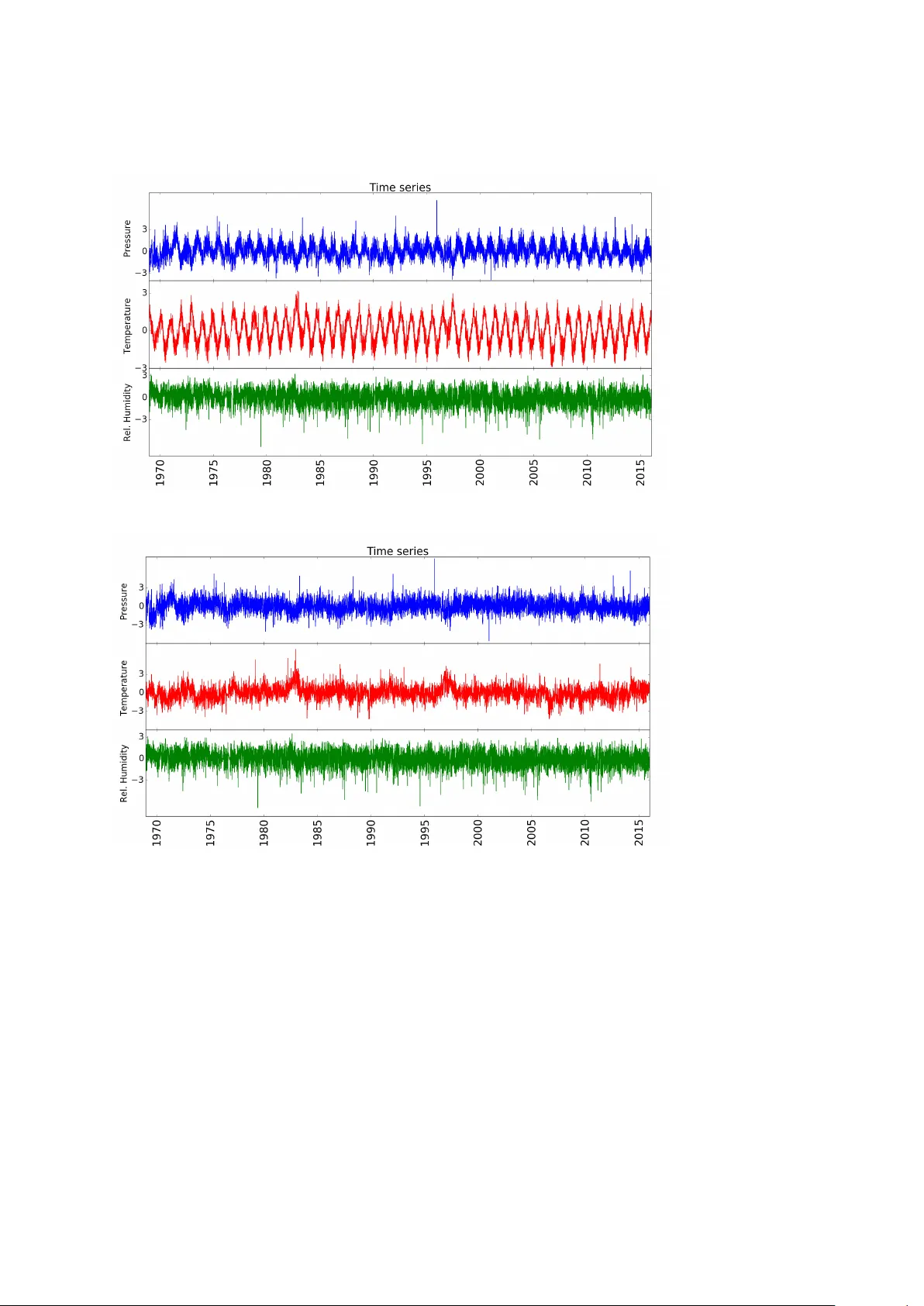
Statistical Analysis of w eather v ariables of An tofagasta H. F arfan † 1 , S. Curilef 1 and A. Castillo 2 1 Departamen to de F ´ ısica, Univ ersidad Cat´ olica del Norte, An tofagasta, Chile. 2 Lab oratorio de Sedim entolog ´ ıa y P aleoam bien tes, Univ ersidad de An tofagasta, Chile. E-mail: † hishan.farfan@ucn.cl Abstract. The statistical behavior of w eather v ariables of An tofagasta is described, esp ecially the daily data of air as temp erature, pressure and relative h umidit y measured at 08:00, 14:00 and 20:00. In this article, we use a time series deseasonalization technique, Q-Q plot, skewness, kurtosis and the Pearson correlation co efficien t. W e found that the distributions of the records are symmetrical and hav e p ositiv e kurtosis, so they hav e heavy tails. In addition, the v ariables are highly auto correlated, extending up to one year in the case of pressure and temp erature. 1. In tro duction It is w ell-known that atmospheric systems essen tially ha ve a non-linear b eha vior due to a large n umber of factors that affect its large-scale evolution as the phenomenon of global atmospheric circulation [1] and small scale as the geographic conditions of the place. An tofagasta is a city lo cated in the north of Chile and its stable climate is due to the almost p ermanen t presence of the Southeast Pacific Subtropical Anticyclone (SPSA), the proximit y of the Andes and the Humboldt curren t. The phenomenon of El Ni ˜ no-Southern Oscillation (ENSO) is also an imp ortan t factor in the dynamics of the atmosphere [2]. The main ob jectiv e of this w ork is to study the statistical b eha vior of the atmospheric v ariables of Antofagasta inspecting the distribution of the data with a Q-Q plot, the skewness and kurtosis, and finally and b y the use of the P earson correlation co efficien t to measure auto correlation. The data used in this study were obtained from the meteorological station in Univ ersidad Cat´ olica del Norte (23.4 ◦ S, 70.2 ◦ W), lo cated at 31 meters ab o v e sea lev el, whose daily records of temp erature, atmospheric pressure and relative humidit y measured since 1969 till 2016 were taken in to accoun t. 2. Meto dology 2.1. Dese asonalization T o remov e the seasonal cycle of a time series, the daily me ans is calculated, whic h is the av erage of the v alues sharing the same day in the y ear. If eac h corresp onding v alue of the original series is subtracted from its corresp onding daily av erage, the resulting v alues are called r esidues . The calculation of deseasonalization is obtained considering ˜ X as the original time series of size N and subtracting the daily a v erages to each corresp onding day d , that is, < ˜ X > d , obtaining the residuals X . X = ˜ X d − D ˜ X E d (1) 2.2. Q-Q plot It is a graphical metho d to compare the probability distribution of a sample to a theoretical distribution of interest (usually normal) by plotting the quan tiles, which are in terv als divide a distribution in to equal p ortions, one distribution against the other. If w e plot the sample data against the generated v alues, a straigh t line with slop e 1 is formed, then both v alues come from the same probability distribution [3]. As an example, figure 2.2 shows the case of three different types of distributions and their resp ectiv e Q-Q plots. In the case of the logistic distribution, it can be seen how the v alues close to the a v erage are underestimated by the normal distribution, and the v alues aw ay from the center they are o verestimated, whereas for the uniform distribution it is the other wa y around, with the cen tral v alues b eing ov erestimated and the extremes underestimated. Figure 1. Histograms with normal fit and normal Q-Q plot of logistic distribution (top), normal dis- tribution (cen ter) and uniform distri- bution (b ottom). 2.3. Skewness and Kurtosis The mean ( µ ) and the v ariance ( σ 2 ) are quantities usually used to describ e the form of a probabilit y distribution, which in turn are derived from a mathematical concept called moment , the first b eing a cen tral measure of the data and the second a measure of the av erage disp ersion around the mean. How ev er, this concept can b e generalized until obtaining momen ts of greater order, suc h as skewness and kurtosis [4], where the first is a measure of symmetry of the distribution around the mean and the second, a measure of the wa y in which the tails of the probabilit y distribution fall (see T able 1). T able 1. Moments of a probabilit y distribution n Name Sym b ol Expression Standard normal distribution 1 Mean µ E ( x ) 0 2 V ariance σ 2 E h ( X − µ ) 2 i 1 3 Sk ewness γ 1 E   X − µ σ  3  0 4 Kurtosis γ 2 E   X − µ σ  4  3 In the case of sk ewness, if after its calculation a p ositiv e v alue is obtained, it is said to hav e p ositiv e skewness and the upper tail falls more slowly than the lo wer one, otherwise, the sk ewness is negativ e. As for kurtosis, if a positive v alue is obtained, the distribution is called L eptokurtic where the tails fall quickly as in the case of the logistic distribution, otherwise if the kurtosis is negativ e, it is called Platykurtic , where its b eha vior is similar to the uniform distribution (see figure 2.2). 2.4. Corr elation c o efficient The Pearson correlation co efficien t is obtained by dividing the co v ariance of t w o v ariables b et w een the pro duct of its standard deviations and calculated as [5]. r = P N i =1 ( x i − µ x ) · ( y i − µ y ) q P N i =1 ( x i − µ x ) 2 · q P N i =1 ( y i − µ y ) 2 , (2) and for t wo series with a certain offset k we get r k = P N − k i =1 ( x i − µ x ) · ( y i + k − µ y ) q P N − k i =1 ( x i − µ x ) 2 · q P N i = k +1 ( y i − µ y ) 2 . (3) This co efficien t is 1 for tw o series with p erfect p ositiv e linear correlation, 0 for statistically indep enden t series and -1 for series with p erfect negative linear correlation. 3. Results W e start by obtaining the r esiduals from the original data sho wn in figure 2 with the deseasonalization method describ ed in equation (1). Observing the graph of the residual data measured at 08:00, whic h are shown in figure 3, the fluctuations of the pressure, temp erature and relative h umidity are evident. A t this p oin t, we can see tw o areas where it is distinguished that the pressure sligh tly decreases and the temp erature considerably increases, these are the ENSO 82-83 and ENSO 97-98. Figure 2. Pressure (top), temp erature (cen tro) and relative h umidity (bottom) measured at 08:00. Figure 3. Residuals of pres- sure (top), temper- ature (cen tro) and relativ e h umidity (b ottom) measured at 08:00. 3.1. Pr ob ability distribution and Q-Q plot In the left part of the figure 3.1 the probability distributions of the residuals of the pressure, temp erature and relative humidit y measured at 08:00 are shown, whose shap es seem to b e normal distributions. On the right side, the Q-Q plot is sho wn as defined in the section 2.2, where the distribution of the three v ariables fits the theoretical normal distribution quite well, except for the v alues farthest from the mean. The fall of the tails of the distributions of the pressure and the temp erature drops quic kly after moving a wa y from the a verage and then falling slowly as they mo ve aw ay from the cen ter, as in the case of the logistic distribution (see figure 2.2). This is corrob orated by the sk ewness ( γ 1 ) and kurtosis ( γ 2 ) v alues (see table 1) of eac h v ariable sho wn in the table 2. The v alue close to zero of the sk ewness of the v ariables is reflected in the symmetry of the distributions around the mean, on the other hand the excessively p ositiv e kurtosis (greater than 3) supp orts the anomalous b eha vior in the fall of the tails in a non-exp onen tial wa y , whic h are commonly kno wn as “hea vy tails” [6], and suggests memory in the records. Figure 4. Probabilit y dis- tribution and Q-Q plot of pressure (top), temp erature (cen ter) and relativ e h umidity (b ottom), measured at 08:00. T able 2. Skewness ( γ 1 ) and Kurtosis ( γ 2 ) of pressure (P A), temp erature (TT) and relativ e h umidity (HR) measured at 08:00, 14:00 and 20:00. P A08 P A14 P A20 TT08 TT14 TT20 HR08 HR14 HR20 γ 1 0.05 -0.02 0.06 0.11 -0.23 0.44 -0.39 0.02 -0.27 γ 2 3.76 3.47 3.48 4.14 8.37 4.36 3.96 3.73 3.69 3.2. Auto c orr elation Using equation (3), the correlogram for the v ariables and the three hours of measuremen t is sho wn in figure 3.2. Autocorrelation b eha vior of the v ariables are different among them; nev ertherless, for each v ariable, the b eha vior itself is similar at all hours. The autocorrelation of the pressure drops abruptly un til appro ximately one month, then slowly decreases to almost zero after appro ximately 10 mon ths. F or temp erature, the fall is even slow er, whose v alues almost v anishes after ab out a y ear, whic h highlights the measurement at 14:00, where after this p eriod the auto correlation barely falls to b e w eak but not zero. In the case of relativ e h umidity , a fast fall is observed after a few weeks, then stabilize un til extremely slo w for 08:00 and 20:00, and in the case of 14:00, the fall after approximately one mon th is imp erceptible, where after a year, the auto correlation is w eak but still p ersisten t. 4. Discussion and Summary The pressure and the temp erature and, to a lesser extent, the relative humidit y , hav e a strong ann ual pattern (see figure 3), whic h w e must remov e to study the v ariables ov er time regardless of the time of y ear. All distributions are symmetric in relation to the mean, but they hav e positive kurtosis (see table 2 and figure 3.1), which indicates that the v ariables are auto correlated, as corrob orated with the analysis of correlation. The main v ariables hav e sho wn correlations that are p ersisten t for several mon ths. F or the pressure and the temp erature last un til the end of the y ear. F or the relativ e humidit y , the correlation remains upto one month. In addition, the pressure and the temp erature endure auto correlated for a long time, while the solar radiation is high, this is, at 14:00 (see figure 3.2). Figure 5. Correlogram of pressure (top), temp erature (cen- ter) and relative h umidity (b ottom). Ac knowledgmen ts W e would lik e to thank partial financial supp ort from FONDECYT 1181558. H.F. is really grateful to F rancisco Calder´ on for the ass i stance in the computer programming. References [1] A. Mak ariev a, V. Gorshko v, A. Nefio do v, D. Sheil, A. Nobre, P . Shearman, and B.-L. Li, “Kinetic energy generation in heat engines and heat pumps: the relationship b et w een surface pressure, temp erature and circulation cell size,” T el lus A: Dynamic Mete or olo gy and Oc eano gr aphy , vol. 69, no. 1, p. 1272752, 2017. [2] R. Garreaud, “The climate of northern Chile: Mean state, v ariability and trends,” R evista Mexic ana de Astr onom ´ ıa y Astr of ´ ısic a , vol. 41, 2011. [3] M. B. Wilk and R. Gnanadesik an, “Probability plotting methods for the analysis of data,” Biometrika , v ol. 55, no. 1, pp. 1–17, 1968. [4] S. Kok osk a and D. Zwillinger, “Crc standard probability and statistics tables and formulae, student edition, mathematics/probabilit y ,” Statistics (L ondon: T aylor and F r ancis) , 2000. [5] P . Cohen, S. G. W est, and L. S. Aiken, Applie d multiple r e gression/c orr elation analysis for the behavior al scienc es . Psychology Press, 2014. [6] S. Asmussen, “Steady-state prop erties of of gi/g/1,” Applie d Pr ob ability and Q ueues , pp. 266–301, 2003.