A convolutional neural network deep learning method for model class selection

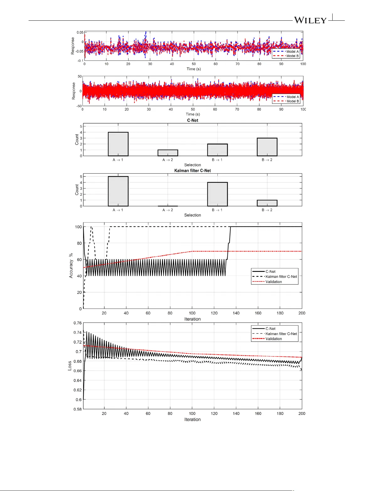
Rece ive d: 16 Jun e 2023 Revised: 27 September 2023 Accepted: 10 November 2023 DOI: 10.1002/eqe.4045 RESEARCH AR TICLE A con volutional neural network deep learning method for model class selection Marios Impraimakis Department of Civil, Maritime and Envir onmental Engineering, University of Southampton, Southampton, UK Correspondence Marios Impraimakis, Department of Civil, Maritime and Environmental Engineering, University of Southampton, Southampton SO16 7QF , UK. Email: m.impraimakis@southampton.ac.uk Abstract The response-only model class selection capability of a novel deep convolutional neural network method is examined herein in a simple, yet effective, manner . Specifically , the responses from a unique degree of freedom along with their class information train and validate a one-dimensional con volutional neural net- work. In doing so , the netw ork selects the model class of new and unlabeled signals without the need of the system input information, or full system iden- tification. An optional physics-based algorithm enhancement is also examined using the Kalman filter to fuse the system response signals using the kinematics constraints of the acceleration and displacement data. Importantly , the method is shown to select the model class in slight signal variations attributed t o the damping behavior or hysteresis behavior on both linear and nonlinear dynamic systems, as well as on a 3D building finite element model, providing a powerful tool for structural health monitoring applications. KEYW ORDS artificial neural networks, con volutional neural networks, machine learning, model class selection-assessment, pattern recognition, physics-enhanced deep learning, structural health monitoring 1 INTRODUC TION The model class selection is an integr al part of the system identification and monitoring process given that either the analytical or the numerical system models are, inevitably , only an appro ximation of the real system. It is particularly useful for engineering systems since it is difficult to be determined solely by the physics due to their empirical nature. The importance of the model class selection, specifically , is highlighted by the fact that a more complicated model fits the data better than one which has fewer adjustable uncertain paramet ers, but it is likely results in data over-fitting and poor future predictions. This is attributed to the parameter fitting which depend too much on the detail of the data and the measurement noise. T o address those challenges, a long history of approaches exists. Akaike 1 introduced a likelihood function which penal- izes the parameterization of the models, and Grigoriu et al. 2 suggested to penalize the complicated models over the simpler ones. Beck and Y uen 3 proposed the ranking of the model classes based on their response conditional probabilities which are calculated by the Bayes’ theorem and the asymptotic expansion of each model class evidence, while Katafygiotis and This is an open access article under the terms of the Creative Commons Attribution License, which permits use, distribution and reproduction in any medium, provided the original work is properly cited. © 2023 The Authors. Earthquake Engineering & Structural Dynamics published by John Wiley & Sons Ltd. 784 wileyonlinelibrary .com/journal/eqe Earthquake Engng Struct Dyn. 2024;5 3:784–814. IMPRAIMAKIS 785 Beck 4 introduced an algorithm to inv estigate the model identifiability in structural model updating using a network of tra- jectories which f inds all other output-equivalent optimal models. Importantly , Ching and Chen 5 developed a simulation- based approach for the simultaneous Bayesian model updating, model class selection, and model a ver aging. Muto and Beck 6 implemented, later , the transitional Mark ov Chain Monte Carlo method for nonlinear structures under seismic loading. Additionally , Cheung and Beck 7 proposed a general method for calculating the model evidence based on the pos- terior samples of the Markov Chain Monte Carlo approach, while Beck 8 inv estigated the Laplace’ s method of asymptotic approximation and the Markov Chain Monte Carlo methods for a structural health monitoring benchmark problem. Furthermore, Raftery et al. 9 developed the method of dynamic model av eraging for online model class selection. Chatzi et al. 10 proposed and experimentally validat ed a twofold criterion based on the smoothness of the parameter prediction and the accuracy of the estimation. Y uen and Mu 11 developed a novel model class selection component into the extended Kalman filter algorithm, to simultaneously provide the model class selection and the parametric identification in a real-time manner . Importantly , Kontoroupi and Sm yth 12 explored how the Bayesian model selection and the unscented Kalman f ilter scheme for joint state and paramet er estimation can be integr ated into a single method using each model’ s probability-plausibility computation. The Bayesian model class selection and the unscented Kalman filter joint scheme with the penalty-type Kullback–Leibler divergence was also investigat ed, 13 and the research is still ong oing. 14– 2 5 However , the curr ent m odel class selection methodologies, apart from the class selection, incorporate also the system identification for each model. The main challenge here is derived from the effort of performing this task for partial unobservable systems, such as larg e systems under very limited information, or systems with unknown inputs. Similarly , this task is not trivial in empirical systems with nonlinear behavior where no acceptable closed-form equation representation exists. A way to address those challenges is examined here using a generalized response-only and (after the training) real-time procedure based on the deep learning capabilities which selects automatically the system model class without having to identify its parameters, measure and estimate all dynamic states, or knowing the system input. The con volutional neural network approach is therefore employed of the deep learning library of methods. Importantly , the con volutional neural networks ha ve already shown an impressive performance on selecting the class of visual imagery data 26 via an ability to recognize patterns. Here, a one- dimensional version is examined for the vibration signals, which has shown a great potentially for damage detection in one or more dimensions. 27–44 The ability to provide the model class selection using a unique degree of freedom (DOF) response measurement, without system identification, and by using a neural network classification approach makes this approach distinctive from the current methodologies. The methodology , specif ically , results in a fast and accurate nonparametric vibration-based tool for model class selection which directly classify the model based solely on response signals. An algorithm enchantment is also inv estigated when the dynamic state estimates of a Kalman filter as developed by Sm yth and W u 45 and implemented as a physics-enhanced kinematics constraint, 46 train a network to recognize their patterns and classify the new and unlabeled signals. In this wa y , the advantages of the Kalman f iltering 47– 55 are explored to improve the performance of the con volutional neural network. Due to the con volutional neur al netw ork ability to learn and extr act the optimal features with a pr oper training, the proposed approach achieves an impressive model class selection accuracy despite the response- only nature of the signals. The work is organized as follows: the Bayesian model class selection and the limitations are overviewed in Section 2 . In Section 3 , the standard convolutional neural network architecture is provided, as well as a comparison of the one- dimensional and the multi-dimensional convolutional neural network versions with a focus on the model class selection. In Section 4 , the Kalman f ilter fusion is formulated for response-only , unknown input, and unknown model class sys- tems. Section 5 provides the summary and the detailed algorithmic tables. Importantly , Sections 6, 7 ,a n d 8 in vestigate numerical applications on both linear and nonlinear dynamic systems, as well as on a 3D building f inite element model. Subsequently , Section 9 presents a discussion, future research sugg estions, and sensitivity analysis for the training process. Finally , the conclusions are provided in Section 10 . 2 BA YESIAN MODEL CLASS SELE CTION T o select the model class 𝕄 𝑖 in a Bayesian framework, one needs to use their prior probability distribution, and then assess their posterior probability plausibility . Let 𝕄 be the space of the models 𝕄 𝑖∶ 𝑖 𝑚𝑎𝑥 . The posterior probability 𝑃(𝕄 𝑖  𝐲, 𝕄 ) of the model class 𝕄 𝑖 is def ined using the Bay es theorem as: 𝑃( 𝕄 𝑖  𝐲, 𝕄 ) = 𝑝( 𝐲  𝕄 𝑖 )⋅𝑃 ( 𝕄 𝑖  𝕄) 𝑝( 𝐲  𝕄) (1) 10969845, 2024, 2, Downloaded from https://onlinelibrary.wiley.com/doi/10.1002/eqe.4045 by University Of Bath, Wiley Online Library on [30/10/2025]. See the Terms and Conditions (https://onlinelibrary.wiley.com/terms-and-conditions) on Wiley Online Library for rules of use; OA articles are governed by the applicable Creative Commons License 786 IMPRAIMAKIS where, 𝑃(𝕄 𝑖  𝕄) is the prior probability of 𝕄 𝑖 , 𝐲 is the measurement vector , and 𝑝(𝐲  𝕄 𝑖 ) is the evidence given the model 𝕄 𝑖 . The denominator is replaced by the summation of the prior probability and the lik elihood for every model class, written as: 𝑃( 𝕄 𝑖  𝐲, 𝕄 ) = 𝑝( 𝐲  𝕄 𝑖 )⋅𝑃 ( 𝕄 𝑖  𝕄)  𝑖 𝑚𝑎𝑥 𝑖  𝑝( 𝐲  𝕄 𝑖 )⋅𝑃 ( 𝕄 𝑖  𝕄)  (2) Let 𝜃 𝑗 ∈𝕄 𝑖 be the parameter 𝑗 of the model 𝕄 𝑖 . The posterior probability distribution 𝑝(𝜃 𝑗  𝐲, 𝕄 𝑖 ) of 𝜃 𝑗 is written as: 𝑝( 𝜃 𝑗  𝐲, 𝕄 𝑖 )= 𝑝( 𝐲  𝜃 𝑗 ,𝕄 𝑖 )⋅𝑝 ( 𝜃 𝑗  𝕄 𝑖 )  𝜃 𝜃 𝜃 𝑝( 𝐲  𝜃 𝑗 ,𝕄 𝑖 )⋅𝑝 ( 𝜃 𝑗  𝕄 𝑖 )𝑑 𝜃 = 𝑝( 𝐲  𝜃 𝑗 ,𝕄 𝑖 )⋅𝑝 ( 𝜃 𝑗  𝕄 𝑖 ) 𝑝( 𝐲  𝕄 𝑖 ) (3) where, 𝑝( 𝐲  𝜃 𝑗 ,𝕄 𝑖 ) is the likelihood given the parameter 𝜃 𝑗 and the model 𝕄 𝑖 ,a n d 𝑝(𝜃 𝑗  𝕄 𝑖 ) is the prior probability density function of 𝜃 𝑗 given the model 𝕄 𝑖 . Here, computing the evidence 𝑝( 𝐲  𝕄 𝑖 ) for each model 𝕄 𝑖 is not trivial. Specifically , the high-dimensional integral is usually analytically intractable, for instance when nonconjugate prior probabilities and/or latent variables exist. T o this end, stochastic simulation methods are used. Particularly , the Markov chain Monte Carlo methods generate samples from the posterior distribution, and then compute the likelihood using the following identity of a rearranged Bay es theorem for every 𝜃 𝑗 : 𝑙𝑛 ( 𝑝( 𝐲  𝕄 𝑖 ) ) =𝑙 𝑛  𝑝( 𝐲  𝜃 𝑗 ,𝕄 𝑖 )  +𝑙 𝑛  𝑝( 𝜃 𝑗  𝕄 𝑖 )  −𝑙 𝑛  𝑝( 𝜃 𝑗  𝐲, 𝕄 𝑖 )  (4) where, the natural logarithm 𝑙𝑛(∙ ) is applied to a void numerical overflows. Equation ( 4 ) is also written as 6 : 𝑙𝑛 ( 𝑝( 𝐲  𝕄 𝑖 ) ) =  𝜃 𝜃 𝜃 𝑙𝑛  𝑝( 𝐲  𝜃 𝑗 ,𝕄 𝑖 )  𝑝( 𝜃 𝑗  𝐲, 𝕄 𝑖 )𝑑 𝜃 𝑑𝜃 𝑑𝜃 −  𝜃 𝜃 𝜃 𝑙𝑛  𝑝( 𝜃 𝑗  𝐲, 𝕄 𝑖 ) 𝑝( 𝜃 𝑗  𝕄 𝑖 )  𝑝( 𝜃 𝑗  𝐲, 𝕄 𝑖 )𝑑 𝜃 𝑑𝜃 𝑑𝜃 (5) where, the first expectation term measures the posterior a verage data fit of the parameter set 𝕄 𝑖 , while the penalty-type second one represents the Kullback–Leibler divergence 56 between the parameter posterior and prior probability distributions. Finally , the identification with the highest evidence 𝑙 𝑛 (𝑝 (𝐲  𝕄 𝑖 )) 12 or the least Kullback–Leibler divergence 13 is selected as the one with the most plausible model class. However , this approach requires a parametric model-based implementation of the model class selection, which inevitably require a parameter estimation and the system input knowledge for input-output identification. Contrastingly in the conv olutional neural network approach, a response-only nonparametric signal-based approach is implemented by using the machine learning means to directly select the model class by recognizing signal patterns. 3 CONV OLUTION AL NEURAL NETW ORK ARCHITE CTURE The con volutional neural networks are a type of deep learning artificial neural network methods with an ability to rec- ognize patterns in visual data. They are composed of multiple building blocks which automatically and adaptively learn spatial hierarchies of features. The one-dimensional con volutional neural networks (1D CNN) ha ve been proven to be highly effective in a variety of signal processing tasks. The fundamental building block of a 1D CNN is the convolutional layer . The conv olutional lay er applies a set of f ilters to the input signal, producing a set of feature maps. The filters ha ve a f ixed size and slide over the input signal, computing a dot product at each location. In doing so, the resulting feature maps capture different aspects of the input signal, such as local trends and patterns. In practice, a 1D CNN may have multiple convolutional layers with different filter sizes and number of f ilters. Each layer can apply a different set of filters to the input signal, allowing the network to capture different aspects of the signal at different scales. The examined one- dimensional convolutional neural network compares to the multi-dimensional counterparts as follows. A one-dimensional configuration fuses the feature extraction and the learning phases of the dynamic states. One-dimensional arrays are used instead of two-dimensional matrices for both the kernels and the feature maps. 10969845, 2024, 2, Downloaded from https://onlinelibrary.wiley.com/doi/10.1002/eqe.4045 by University Of Bath, Wiley Online Library on [30/10/2025]. See the Terms and Conditions (https://onlinelibrary.wiley.com/terms-and-conditions) on Wiley Online Library for rules of use; OA articles are governed by the applicable Creative Commons License IMPRAIMAKIS 787 Additionally , the network architecture has the hidden neurons of the conv olution layers which perform both the con vo- lution and the sub-sampling operations. The fully-connected layers are identical to the hidden lay ers of the multi-lay er perceptrons where the classification task is mainly realized. Accordingly , the multi- dimensional matrix manipulations, namely the con volution and the lateral rotation, are replaced by their one-dimensional counterparts, namely the conv olution and the reverse oper ations. Finally , the par ameters for the kernel size and the sub- sampling are scalars. Importantly , this simplif ied structure of the convolution neural network requires only one- dimensional con volutions and therefore, a mobile and low- cost hardwar e implementation for near real-time applications. The algorithmic details of the 1D CNN are provided in Section 5 . A short description of the additional layers in the convolutional neural network architecture is provided. Input Layer : The layer where the input is specified. Convolutional Layer : The layer where the filters are applied to the input, usually between a subarra y of the input array and the filter , and where the neurons connect to the input subarra y . In this layer , the number of feature maps is also determined. Batch Normalization Layer : The lay er where the normalization of the activations and gradients occurs leading to a simpler optimization training problem. It is usually followed by a nonlinear activation function. P ooling Layer : The layer where the down-sampling oper ation is applied to reduce the spatial size of the feature map and to remove the redundant spatial information. This leads to an increase of the number of filters in deeper con volutional layers without increasing the required amount of computation per layer . Fully Connected Layer : The la yer where the neurons connect to the neurons in the preceding la yer to combine all the features learned by the previous layers and identify the larger patterns. Importantly , the last fully connected layer combines the features to classify the data and is equal to the number of classes in the input data. Softmax Layer : The layer where the activation function normalizes the output of the fully connected la yer . The output of this lay er consists of positive numbers that sum to one, which are then used as classification probabilities by the classification la yer . Classification Lay er : The final lay er where the probabilities are returned by the activation function for each input to assign the mutually exclusive classes and compute the loss. Importantly , the training of the network is implemented usually by a stochastic gradient descent with a specif ied number of epochs, where an epoch is a full training cycle on the entire training data set. In this work, the one-dimensional convolutional approach is applied to select the model class. The examined approach fuses both the feature extraction and the classif ication blocks into a single and compact learning body . The advantage is the ability to extr act optimal model class-sensitive features automatically from the response-only signals. 4 RESPONSE- ONL Y AND UNKNOWN MODEL CLASS D YNAMIC ST A TE ESTIMA TION USING THE KALMAN FIL TER F or a further improv ement of the 1D CNN performance with r esponse-only signals when additional signals are avail- able, the Kalman filter data fusion technique may be used by Smyth and Wu. 45,46 The Kalman filter alg orithm, given a series of noisy measurements observed over time, estimates optimally the system dynamic states using a joint probability distribution over the states for each timeframe. The algorithm works in two steps: the first step is the prediction of the dynamic states using the dynamic process model which also propagates the uncertainty of the dynamic states. The second update step incorporates the measurements to calibrate the dynamic state estimation using a weighted aver ag e strategy , where more weight is given to the estimates with higher certainty . The alg orithm is recursive and it is used online and, potentially , with real-time data. Ev en for simple systems though, the knowledge of the system parameters and input is needed to predict future steps. This leads to an una vailability of filtering the signals when response-only and unknown model class scenarios are examined. T o this end, the dynamic states are filtered using acceleration and displacement measurements 45,46 as:   𝑥  𝑥  =  01 00  𝑥  𝑥  +  0 1  𝑎+  0 1  𝜂 𝑎 (6) 𝑦= 𝑑= [ 1 0 ]  𝑥  𝑥  +𝜂 𝑑 (7) where, 𝑎 and 𝑑 are the acceler ation and displacement measurements, respectively , and 𝜂 𝑎 and 𝜂 𝑑 are their associated noise. It is assumed that 𝜂 𝑎 and 𝜂 𝑑 are white noise Gaussian processes. By introducing the state variables, 𝐱=  𝑥 1 𝑥 2  =  𝑥  𝑥  (8) 10969845, 2024, 2, Downloaded from https://onlinelibrary.wiley.com/doi/10.1002/eqe.4045 by University Of Bath, Wiley Online Library on [30/10/2025]. See the Terms and Conditions (https://onlinelibrary.wiley.com/terms-and-conditions) on Wiley Online Library for rules of use; OA articles are governed by the applicable Creative Commons License 788 IMPRAIMAKIS Equations ( 6 )a n d( 7 ), without the noise terms, are writt en in matrix form as:  𝐱=𝐀 𝐱 + 𝐁 𝑎 (9) 𝑦= 𝐇 𝐱 (10) If acceleration measurements are a vailable at intervals of Δ𝑡 , the process Equation ( 9 ) and the observation Equation ( 10 ) are discretized as: 𝐱(𝑘 + 1) = 𝐀 𝐝 𝐱(𝑘 ) + 𝐁 𝐝 𝑎( 𝑘) (11) 𝑦 (𝑘 + 1) = 𝐇 𝐱(𝑘 + 1) (12) namely ,  𝑥 1 (𝑘 + 1) 𝑥 2 (𝑘 + 1)  =  1Δ 𝑡 01  𝑥 1 (𝑘 ) 𝑥 2 (𝑘 )  +  Δ𝑡 2 ∕2 Δ𝑡  𝑎( 𝑘) +  Δ𝑡 2 ∕2 𝛿𝑡  𝜂 𝑎 (𝑘 ) (13) 𝑦= [ 1 0 ]  𝑥 1 (𝑘 + 1) 𝑥 2 (𝑘 + 1)  +𝜂 𝑑 (𝑘 + 1) (1 4) where 𝑘 step stands for the 𝑘⋅Δ 𝑡 time instance. In the approach of Equation ( 13 ), a physics-enhanced fusion of the displacement and the acceleration signals is imple- mented. Specifically , the object kinematics equation is employed as the system pseudo-model to provide the physical relationship between the displacement and acceleration data, without incorporating any knowledge of the actual system model and its class. Equation ( 13 ) is simpler written using the well-known body-motion equations as: Physical Kinematics Model =      𝑥 2 =𝑥 2 + 1 2 𝑎⋅ Δ 𝑡 𝑥 1 =𝑥 1 +𝑥 2 ⋅Δ 𝑡 + 1 2 𝑎⋅ Δ 𝑡 2 (15) where, the acceleration 𝑎 is assumed to be constant between each sequential steps; an assumption which does not lead to divergences due to the small value of Δ𝑡 . Overall, this fusion algorithm uses the Kalman filter which, given acceleration and displacement measurements, pro- vides optimally the displacement and the velocity dynamic states. Importantly , the displacement measurement is provided by the integration of the acceleration signal on linear systems. The obtained results can be used instead of ra w signals to train, validate, and test the convolutional neural network for model class selection. Notably , those response-only signals are used as input data to the network, and they should not be confused with the output of the network. Finally , the one- dimensional conv olutional neural network pr ocedure for model class selection is implemented as follows. The dynamic states of a unique system responses are loaded to tr ain and validate the network. Importantly , these signals are already labeled with the model class. The one-dimensional convolutional neural network architecture is defined where the input size of the training data is specif ied as the number of their classes. Subsequently , the network training optimization algorithm is specified which included a mini-batch approach with an adequate number of epochs. F or online purposes with a unique response training signal, the mini-batch size is set equal to 1, otherwise larger v alues also are used. Once the network is trained, it is used to evaluate the new and unlabeled signals, and select their model class. Importantly , no additional data such as the system input or the system paramet ers are needed. 5 PROCEDURE SUMMAR Y The overall procedur e is illustrated here where each step is detailed in T able 1 : 1. Initialize the measurement filtering (optional for improved performance incorporating more data) . Set the initial probability distributions f or the dynamic states of each mode class response signal. 10969845, 2024, 2, Downloaded from https://onlinelibrary.wiley.com/doi/10.1002/eqe.4045 by University Of Bath, Wiley Online Library on [30/10/2025]. See the Terms and Conditions (https://onlinelibrary.wiley.com/terms-and-conditions) on Wiley Online Library for rules of use; OA articles are governed by the applicable Creative Commons License IMPRAIMAKIS 789 TA B L E 1 Kalman f ilter convolutional neural network (Kalman filter C-Net). Step 1 (optional): ∙ Initialize the dynamic state estimation: ∙𝑘 = 0 (Time step) ∙𝐱 𝐤 =𝔼 [ 𝐱 𝟎 ] ( 𝔼 stands for Expectation) ∙𝐏 𝐤 =𝔼 [ ( 𝐱 𝟎 −𝐱 𝐤 )(𝐱 𝟎 −𝐱 𝐤 ) 𝑇 ] (Covariance matrix) Step 2 (optional): ∙ Predict and estimate the dynamic states: ∙𝐱 𝐤+ 𝟏 =𝐀 𝐝 𝐱 𝐤 +𝐁 𝐝 𝑎 𝑘 (prediction) ∙𝐏 𝐤+ 𝟏 =𝐀 𝐝 𝐏 𝐤 𝐀 𝐓 𝐝 +𝐐 𝐝 ∙𝐉 = 𝐏 𝐤+ 𝟏 𝐇 𝐓 (𝐑 𝐝 +𝐂 𝐏 𝐤+ 𝟏 𝐇 𝐓 ) −1 ∙𝐱 𝐤+ 𝟏 =𝐱 𝐤+ 𝟏 +𝐉 ( 𝐲 𝐤+ 𝟏 −𝐇 𝐱 𝐤+ 𝟏 ) (estimation) ∙𝐏 𝐤+ 𝟏 =( 𝐈 −𝐉 𝐇 ) 𝐏 𝐤+ 𝟏 (𝐈 − 𝐉 𝐇) 𝑇 +𝐉 𝐑 𝐝 𝐉 𝑇 ∙ Repeat Step 2 for 𝑘=𝑘 + 1 until 𝑘 𝑚𝑎𝑥 Step 3: ∙ Initialize randomly all weights for the neural network ∙ Forw ard propagate the input data: ∙𝐳 𝐡 𝐣 =𝑏 ℎ 𝑗 +  ℎ−1 𝑖=1 𝐷( 𝑣 𝑖𝑗 ,𝐬 𝐡−𝟏 𝐢 ) ∙𝐮 𝐡 𝐣 =𝐹 ( 𝐳 𝐡 𝐣 ) and 𝐬 𝐡 𝐣 =𝐮 𝐡 𝐣 downsampling ∙ Compute the delta error at the output layer and back-propagate it: ∙𝐸 =  𝑁 ℎ ℎ=1 (𝐮 𝐍 𝐡 𝐡 −𝐫 𝐡 ) 2 ∙𝜕 𝐸∕ 𝜕𝑣 ℎ−1 𝑖𝑗 =Δ ℎ 𝑗 𝐮 𝐡−𝟏 𝐢 and 𝜕𝐸 ∕ 𝜕𝑏 ℎ 𝑗 =Δ ℎ 𝑗 ∙𝜕 𝐸∕ 𝜕𝑠 ℎ 𝑗 =  𝑁 ℎ +1 ℎ=1 Δ ℎ+1 ℎ 𝑣 𝑗ℎ Step 4: ∙ Post-process to compute the weight and bias sensitivities: ∙Δ 𝑗 ℎ =𝜕 𝐸 ∕ 𝜕 𝐮 𝐡 𝐣 ⋅𝜕 𝐮 𝐡 𝐣 ∕ 𝜕𝐳 𝐡 𝐣 (further back propagation) ∙ Update the weights and biases with the accumulation of sensitivities: ∙𝑣 ℎ−1 𝑖𝑗 (𝑡 + 1) = 𝑣 ℎ−1 𝑖𝑗 ( 𝑡 ) −𝜖 ⋅ 𝜕𝐸∕𝜕𝑣 𝑖𝑗 (adaptive 𝜖 ≈ 0.001 ) ∙𝑏 ℎ 𝑗 (𝑡 + 1) = 𝑏 ℎ 𝑗 (𝑡 ) − 𝜖 ⋅ 𝜕 𝐸 ∕ 𝜕 𝑏 ℎ 𝑗 Step 5: ∙ Move to each next layer until the network is fully trained. Classify the unlabeled signals from Step 3 using the trained network. 2. Filter the dynamic states online (optional for improved performance incorporating more data) . Predict the dynamic states using the acceler ation measurements and the discr ete state-space modeling. Estimate the dynamic states using the displacement measurements. The displacement measurements may have a different rate than accelera- tion measurements. 45,46 Importantly , for linear systems double-integrate the acceleration measurements. Also, Re pe at the filtering for the full signal duration . Repeat the Kalman f ilter procedure for all time steps to provide the full input. 3. F eed the network . Provide the one- dimensional conv olutional neural network with the raw signals or filtered sig- nals from Step 2 associated with their model class. At this point, generate randomly the weights of the network. Also, Initialize the network training . Start the network training where the signal data are propagat ed between the lay ers. 4. Implement the back-propagation algorithm in the network training . P ost-process the signal data for the estima- tion of the weights and bias sensitivities. Update the weights and biases with the accumulation of sensitivities. Finally , move to each next layer . 5. Select the model class . Use the trained network to classify the unlabeled signals. Specifically , provide the new , unused, and unlabeled ra w or filtered signals from Step 2 as an input to the network to output the model class. 10969845, 2024, 2, Downloaded from https://onlinelibrary.wiley.com/doi/10.1002/eqe.4045 by University Of Bath, Wiley Online Library on [30/10/2025]. See the Terms and Conditions (https://onlinelibrary.wiley.com/terms-and-conditions) on Wiley Online Library for rules of use; OA articles are governed by the applicable Creative Commons License 790 IMPRAIMAKIS TA B L E 2 Damping kernel functions 𝑔(𝑡) for the generalized damping model classes. Kernel function 𝒈(𝒕) Constraints ∙𝜇 1 𝑒 −𝜇 1 𝑡 𝜇 1 ,𝑡  0 ∙( 𝜇 2 ) 2 𝑡𝑒 −𝜇 2 𝑡 𝜇 2 ,𝑡  0 ∙2  𝜇 3 𝜋 𝑒 −𝜇 3 𝑡 2 𝜇 3 ,𝑡  0 ∙  1∕𝜇 4 0 0<𝑡<𝜇 4 𝑡>𝜇 4 𝑛𝑜 ∙      1 𝜇 5 [1 + cos( 𝜋𝑡 𝜇 5 )] 0 0<𝑡<𝜇 5 𝑡>𝜇 5 𝑛𝑜 ∙ 𝛿(𝑡 ) 𝑡  0 ∙ any 𝑔(𝑡)  Energy dissipation >0  ∞ 0 𝑔(𝑡) 𝑑𝑡 = 1, 𝑡  0 In T able 1 , 𝐳 𝐡 𝐣 is the network input at layer ℎ and neuron 𝑗 , 𝑏 𝑗 is a scalar bias, and 𝐬 𝐢 is the output of the neuron 𝑖 at the layer ℎ−1 . Also , 𝑣 𝑖𝑗 is the k ernel weight from the neuron 𝑖 at layer ℎ− 1 to the neuron 𝑗 at la yer ℎ ,a n d 𝐮 𝐡 𝐣 is the intermediate output. Related to the back propag ation of the error starting from the output fully connected layer , 𝑁 ℎ is the number of classes in the input data, and 𝐫 𝐡 corresponds to the target and output vector . Finally , the delta of the neuron 𝑗 at la yer ℎ , Δ ℎ , is used to update the bias of that neuron, as well as, all the weights of the neurons in the previous layer connected to that neuron. 6 APPLICA TION TO LINEAR D YNAMIC SYSTEMS F or the linear numerical application consider the case of the damping model classes in structural dynamics. The standard equation of motion of a 𝑛 DOF structural-mechanical system, in the case of proportional damping, is written as: 𝐌 𝐱 ( 𝑡 )+𝐂  𝐱 ( 𝑡) + 𝐊 𝐱( 𝑡) = 𝐟 ( 𝑡) (16) where, 𝐌 and 𝐊 are the mass and stiffness matrices, respectively , and 𝐂 is the proportional to 𝐌 and/or 𝐊 damping matrix that satisf ies the orthogonality property . This means that if 𝚽 is the matrix that contains the eigenv ectors of the system, then 𝐂=𝚽 𝑇 𝐂𝚽 is a diagonal matrix and thus, a decoupling procedure can be implemented. Here, 𝐱(𝑡 ) and 𝐟( 𝑡 ) are the response of the system and the force applied to the system, respectively . With regar d to damping the form of Equation ( 16 ) is restrictive, and for a general consideration of structural-mechanical systems, alternatively damping model classes are considered. This is implemented by one or more conv olution integrals over a k ernel function 𝑔(𝑡) . In doing so, the damping depends on the past history of the motion. The equation of motion then is written as an integro-differential equation: 𝐌 𝐱 ( 𝑡 )+𝐂 𝑡  0 𝑔(𝑡 − 𝜏 )  𝐱(𝜏) 𝑑 𝜏 + 𝐊 𝐱(𝑡 ) = 𝐟 (𝑡 ) (1 7) where, this formulation is a generalization of the standard damping modeling since by using the Kroneck er delta function 𝛿( 𝑡) as the k ernel function 𝑔(𝑡) ,E q u a t i o n( 17 ) reduces to Equation ( 16 ). F or the choice of the damping kernel functions, man y candidate functions may be considered. Observations, though, from real systems 57 suggest that the exponential function can often adequately model the damping, and is a natural choice. Ta b l e 2 shows several candidate kernel functions 13,58 which have been shown to adequately model the damping beha v - ior of structural-mechanical systems. Here, 𝜇 𝑖 is damping model paramet er which is properly calibr ated by system identification procedures. 13 10969845, 2024, 2, Downloaded from https://onlinelibrary.wiley.com/doi/10.1002/eqe.4045 by University Of Bath, Wiley Online Library on [30/10/2025]. See the Terms and Conditions (https://onlinelibrary.wiley.com/terms-and-conditions) on Wiley Online Library for rules of use; OA articles are governed by the applicable Creative Commons License IMPRAIMAKIS 791 The syst em of Equation ( 17 ) is then examined with va rious model classes. Specifically , the system matrices for the synthetic measurement generation are: 𝐌=  𝑚 1 0 0𝑚 2  =  10 01  ,𝐂 =  𝑐 1 +𝑐 2 −𝑐 2 −𝑐 2 𝑐 2  =  1+2 − 2 −2 2  , 𝐊=  𝑘 1 +𝑘 2 −𝑘 2 −𝑘 2 𝑘 2  =  9 + 11 −11 −11 11  (18) with the initial conditions are 𝐱(0) = [1 1] 𝑇 and  𝐱(0) = [0 0.5] 𝑇 . White noise is chosen for the force 𝐟( 𝑡 ) = [𝑓 1 (𝑡 ) 𝑓 2 (𝑡 )] 𝑇 of mean value 0 and variance 9. Importantly , the initial conditions and/or the for ce should be chosen to excite the system sufficiently . Three model classes are considered with three different kernel functions, namely: 1. 𝑔 ( 𝑡 )=𝜇 1 𝑒 −𝜇 1 𝑡 with 𝜇 1 =1 . 5 (Model A) 2. 𝑔 ( 𝑡 )=2  𝜇 3 𝜋 𝑒 −𝜇 3 𝑡 2 with 𝜇 3 =1 . 5 (Model B) 3. 𝑔 ( 𝑡 )=𝛿 ( 𝑡 ) (Model C) T o create synthetic measurements, the integration method of Katsikadelis 13,59 ,60 is implemented as: 𝐳 𝐤 =𝐅 𝐤 ⋅𝐳 𝐤− 𝟏 +𝐁 𝐤 ⋅𝐮 𝐤 (19) where: i) 𝐳 𝐤− 𝟏 =[  𝐱 𝐤− 𝟏  𝐱 𝐤− 𝟏 𝐰 𝐤− 𝟏 𝐱 𝐤− 𝟏 ] 𝑇 ii) 𝐮 𝐤 =[ 𝐟 𝐤 𝟎 𝟏×𝐧 𝟎 𝟏×𝐧 𝐟 𝐰 𝐤 ] 𝑇 iii) 𝐰 𝐤− 𝟏 =  𝑘−2 𝑖= 1 𝑊 𝑖 ⋅( 𝐱 𝐢 + 𝐱 𝐢−𝟏 )∕2 + 𝑊 𝑘−1 ⋅( 𝐱 𝐤− 𝟏 + 𝐱 𝐤− 𝟐 )∕2 iv) 𝑊 𝑖 =  (𝑖 )Δ𝑡 (𝑖 −1)Δ𝑡 𝑔(𝑘 ⋅ Δ𝑡 − 𝜏) 𝑑𝜏 v) 𝐟 𝐰 𝐤 =  𝑘−1 𝑖= 1 𝑊 𝑖 ⋅( 𝐱 𝐢 + 𝐱 𝐢−𝟏 )∕2 vi) 𝐅 𝑘 =       𝐌 𝐧×𝐧 𝟎 𝑛×𝑛 𝐂 𝑛×𝑛 𝐊 𝑛×𝑛 Δ𝑡 2 ∕4 ⋅𝐈 𝑛×𝑛 −Δ𝑡 ⋅𝐈 𝑛×𝑛 𝟎 𝑛×𝑛 𝐈 𝑛×𝑛 −Δ𝑡∕2 ⋅𝐈 𝑛×𝑛 𝐈 𝑛×𝑛 𝟎 𝑛×𝑛 𝟎 𝑛×𝑛 𝟎 𝑛×𝑛 −𝑊 𝑘 ∕2 ⋅𝐈 𝑛×𝑛 𝐈 𝑛×𝑛 𝟎 𝑛×𝑛       −1       𝟎 𝐧×𝐧 𝟎 𝑛×𝑛 𝟎 𝑛×𝑛 𝟎 𝑛×𝑛 −Δ𝑡 2 ∕4 ⋅𝐈 𝑛×𝑛 𝟎 𝑛×𝑛 𝟎 𝑛×𝑛 𝐈 𝑛×𝑛 Δ𝑡∕2 ⋅𝐈 𝑛×𝑛 𝐈 𝑛×𝑛 𝟎 𝑛×𝑛 𝟎 𝑛×𝑛 𝟎 𝑛×𝑛 𝑊 𝑘 ∕2 ⋅𝐈 𝑛×𝑛 𝟎 𝑛×𝑛 𝟎 𝑛×𝑛       vii) 𝐁 𝑘 =       𝐌 𝐧×𝐧 𝟎 𝑛×𝑛 𝐂 𝑛×𝑛 𝐊 𝑛×𝑛 Δ𝑡 2 ∕4 ⋅𝐈 𝑛×𝑛 −Δ𝑡 ⋅𝐈 𝑛×𝑛 𝟎 𝑛×𝑛 𝐈 𝑛×𝑛 −Δ𝑡∕2 ⋅𝐈 𝑛×𝑛 𝐈 𝑛×𝑛 𝟎 𝑛×𝑛 𝟎 𝑛×𝑛 𝟎 𝑛×𝑛 −𝑊 𝑘 ∕2 ⋅𝐈 𝑛×𝑛 𝐈 𝑛×𝑛 𝟎 𝑛×𝑛       −1 Here, the time discretization frequency is set equal to 100 Hz, therefore Δ𝑡 is 0.01. The same holds for the sampling frequency of the synthetic measurements. Finally , to consider the effect of measurement noise, each response signal is contaminated by a Gaussian white noise sequence with a 10% root-mean-square noise-to-signal ratio. Different ini- tial conditions are applied to the system to generate multiple responses for training and v alidation. The duration of the acceleration and displacement signal measurement for each model class is 40 s. T o Kalman filter all previous signals, the process covariance 𝐐 𝐝 and the measurement cov ariance 𝐑 𝐝 matrices ar e chosen to be constant during the identification process and equal to 10 −9 ⋅𝐈 𝟐×𝟐 and 10 −3 ⋅𝐈 𝟏×𝟏 , respectively . F or larger values, the algorithm needs more data and time to conv erge, or it may even diverge. The convolutional neural network architecture is defined as follows in Figure 1 : An input layer with the three signals for each one of the three model classes A, B, and C, associated with their model class label. A con volutional layer is set with filter size equal to 2048 and number of neurons that connect to the same region of the input equal to 128 with casual padding. A rectifier layer , termed also as R eLu is also set, as well as a batch normalization layer with mini-Batch size equal to 1 for online purposes, and an additional convolutional la yer with filter size equal to 2048 and number of neurons 10969845, 2024, 2, Downloaded from https://onlinelibrary.wiley.com/doi/10.1002/eqe.4045 by University Of Bath, Wiley Online Library on [30/10/2025]. See the Terms and Conditions (https://onlinelibrary.wiley.com/terms-and-conditions) on Wiley Online Library for rules of use; OA articles are governed by the applicable Creative Commons License 792 IMPRAIMAKIS FIGURE 1 Examined C-Net architecture for all numerical applications. that connect to the same region of the input equal to 256 with casual padding. An additional rectifier lay er is set along with an additional batch normalization la yer with mini-Batch size equal to 1, and a global aver age pooling layer . Finally , a fully connected lay er is set with a n umber of classes equal to 3, a softmax layer , and a classif ication layer . Importantly , an investig ation of the number of the filter size and the number of neurons within the con volutional lay er is shown in Section 9 . Last but not least, the number of the maximum epochs in the optimization process is set equal to 15. Importantly , to design the architecture, although still an active research problem, 61 a simple CNN architecture is examined that h as one hidden layer with one max pooling layer before the classification one. Based on the results and by controlling the trade-off between accuracy and training speed, the number of k ernels and lay ers is increased until a satisfactory performance is reached. This work uses similar architecture building philosophy to the damage detection applications 28,32 without an y special adjustments that would potentially fa vor the model class selection problem. T wo signal inputs are examined in Figures 2–3 . In these figures, the first and second row refer to the displacement and acceleration ra w signal used in the Kalman filter for all models. The third row refers to the network model class selection trained with unf iltered signals (C-Net) where the data g enerat ed by model A denoted by 1, model B denoted by 2, and model C denoted by 3 are attributed to each model A, B, or C. Similarly , the fourth row refers to the network model class selection trained with the Kalman filtered signals (Kalman filter C-Net). Additionally , the fifth row refers to the accuracy in the training process for both networks with respect to the number of optimization iterations, while the sixth row refers to the loss in the training process for both networks with respect to the number of optimization iterations. In total, 9 new velocity and displacement signals are classified, where ideally the first 3 signals belong to Model A, the second 3 signals belong to Model B, and the last 3 signals belong to Model C. In Figure 2 , the performance of the networks using only the DOF 2 displacement signals in the training and v alidation process is shown. The C-Net correctly selects the model class for each signal. The Kalman filter C-Net also correctly selects the model class for each signal, but with a shorter training period and loss minimization than C-Net. In Figure 3 , the performance of the networks using only the DOF 2 velocity signals in the training and validation process is shown. Both networks select correctly the model class for each signal expect one. Importantly , the Kalman filter C-Net conv erges faster . Importantly , in this application, it ma y seem that the model is quite simple and, perhaps, does not need such a complex network in the prediction, meaning the conv olution neural network is not efficiently designed. In reality though, removing lay ers from the network results in a poorer performance where the predictions are wrong. Additionally , it may seem that the model classes are too idealized since the model class can be well depicted by the mathematical formulas in T able 2 . In reality though, those models hav e been experimentally demonstrated that they represent the beha vior of real dynamic systems, that is, chap . 8 of Adhikari. 57 7 APPLICA TION TO NONLINEAR D YNAMIC SYSTEMS F or the nonlinear n umerical application consider initially the problem of a mass in free fall 62 landing on a generalized damped base material. The stiffness and damping elements of the base material are active only when the body is in contact 10969845, 2024, 2, Downloaded from https://onlinelibrary.wiley.com/doi/10.1002/eqe.4045 by University Of Bath, Wiley Online Library on [30/10/2025]. See the Terms and Conditions (https://onlinelibrary.wiley.com/terms-and-conditions) on Wiley Online Library for rules of use; OA articles are governed by the applicable Creative Commons License IMPRAIMAKIS 793 FIGURE 2 System of Section 6 : Results for the linear dynamic system when training and validating with the DOF 2 displacement signals. First and second row: the displacement and acceleration raw signals in m/s and m/s 2 , respectively . Third row: C-Net model class prediction where ideally A- > 1, B- > 2, and C- > 3. Fourth row: Kalman filter C-Net model class prediction. Fifth and six row: accuracy and loss in the training process for both networks. 10969845, 2024, 2, Downloaded from https://onlinelibrary.wiley.com/doi/10.1002/eqe.4045 by University Of Bath, Wiley Online Library on [30/10/2025]. See the Terms and Conditions (https://onlinelibrary.wiley.com/terms-and-conditions) on Wiley Online Library for rules of use; OA articles are governed by the applicable Creative Commons License 794 IMPRAIMAKIS FIGURE 3 System of Section 6 : Results for the linear dynamic system when training and validating with the DOF 2 velocity signals. First and second row: the displacement and acceleration ra w signals in m/s and m/s 2 , respectively . Third row: C-Net model class prediction where ideally A- > 1, B- > 2, and C- > 3. Fourth row: Kalman filter C-Net model class prediction. Fifth and six row: accuracy and loss in the training process for both networks. DOF , degree of freedom. 10969845, 2024, 2, Downloaded from https://onlinelibrary.wiley.com/doi/10.1002/eqe.4045 by University Of Bath, Wiley Online Library on [30/10/2025]. See the Terms and Conditions (https://onlinelibrary.wiley.com/terms-and-conditions) on Wiley Online Library for rules of use; OA articles are governed by the applicable Creative Commons License IMPRAIMAKIS 795 with it. The equation of motion is nonlinear and it is expressed as: 𝑚  𝑥( 𝑡) + 𝐺 ( 𝑥( 𝑡) , 𝜃 ) =𝑓 ( 𝑡 ) (20) and if, for instance, the effectiveness of a twofold model is examined, then the equation of motion is written as: 𝑚  𝑥 ( 𝑡 )+ℍ ( 𝑥( 𝑡) ) ⋅      𝑐⋅ 𝑡  0 𝛿( 𝑡 − 𝜏)  𝑥( 𝜏) 𝑑𝜏 + 𝑐 ⋅ 𝑡  0 𝑔(𝑡 − 𝜏 )  𝑥( 𝜏) 𝑑𝜏 + 𝑘 𝑥(𝑡)      =𝑓 ( 𝑡 ) (21) where, ℍ(𝑥 (𝑡 )) is the Heaviside step function. Assume here, 𝑚=1 Kg, 𝑐=3 Ns / m , 𝑘 = 1000 N/m, 𝑓( 𝑡) = − 𝑚𝑔 with 𝑔 = 9.81 𝑚 ∕𝑠 2 for the gra vity acceleration. The initial conditions are 𝐱(0) = 0.1 and  𝐱(0) = 0 . White noise is chosen for the force 𝐟( 𝑡 ) of mean value 0 and variance 9. Importantly , the initial conditions and/or the force should be chosen to excite the system suff iciently . T wo model classes are considered for the 𝑔(𝑡) in Equation ( 21 ) with two different kernel functions, namely: 1. 𝑔 ( 𝑡 )=𝜇 1 𝑒 −𝜇 1 𝑡 with 𝜇 1 = 100 (Model A) 2. 𝑔 ( 𝑡 )=2  𝜇 3 𝜋 𝑒 −𝜇 3 𝑡 2 with 𝜇 3 = 100 (Model B) T o create synthetic measurements, the integration method of Katsikadelis 13,59 ,60 is implemented as in Section 6 where, for nonlinear systems, the state transition matrix 𝐅 𝐤 and the input matrix 𝐁 𝐤 are modified and in the stead of 𝐂 𝑛×𝑛 and 𝐊 𝑛×𝑛 , the zero matrix 𝟎 𝑛×𝑛 is inserted. Also, the new input is: 𝐮 𝐤 = [(𝐟 𝐤 −𝐟 𝐧 𝐤 )𝟎 𝟏×𝐧 𝟎 𝟏×𝐧 𝐟 𝐰 𝐤 ] 𝑇 (22) where, a system of equations provides the numerical solution of the nonlinear system, namely:  𝐳 𝐤 =𝐅 𝐤 ⋅𝐳 𝐤− 𝟏 +𝐁 𝐤 ⋅𝐮 𝐤 𝐟 𝐧 𝐤 =𝐆 ( 𝐳 𝐤 ,𝜃 𝑘 𝜃 𝑘 𝜃 𝑘 ) (23) Here, the time discretization frequency is set equal to 100 Hz, therefore Δ𝑡 is 0.01. The same holds for the sampling frequency of the synthetic measurements. Finally , to consider the effect of measurement noise, each response signal is contaminated by a Gaussian white noise sequence with a 10% root-mean-square noise-to-signal ratio. The duration of the acceleration and displacement signal measurement for each model class is 100 s. T o Kalman f ilter the signals, the process covariance 𝐐 𝐝 and the measurement covariance 𝐑 𝐝 matrices are chosen to be constant during the identif ication process and equal to 10 −9 ⋅𝐈 𝟐×𝟐 and 10 −3 ⋅𝐈 𝟏×𝟏 , respectively . F or larg er values, the algorithm needs more data and time to converge, or it may even diverge. Subsequently , the network architecture is defined similarly to Section 6 . T wo signal inputs are examined in Figures 4–5 with the same la yout description as in Section 6 . In total, 10 new velocity and displacement signals are classif ied, where ideally the first 5 signals belong to Model A, and the second 5 signals belong to Model B. In Figure 4 , the performance of the networks using only the DOF 1 displacement signals in the training and validation process is shown. The C-Net correctly selects the model class for each signal apart from one which is misclassified as Model A despite belonging to Model B. The Kalman filter C-Net also provides the same selection accuracy , but with a shorter training period and loss minimization. In Figure 5 , the performance of the networks using only the DOF 1 velocity signals in the training and validation process is shown. The C-Net selects correctly the class of seven signals, but misselects three of them. Contrastingly , the Kalman filter C-Net misselects only 1 signal out 10. In this examination, the Kalman f ilter C-Net shows a superior performance compared to C-Net in the selection accuracy , apart from solely a faster con vergence. Furthermore, for the nonlinear numerical application to other model class types and not only in damping kernels such as on the stiffness matrix, 63 consider a 6-story shear type model extending the application of Kontor oupi and Smyth. 12,47 Here, the first DOF is associated with a nonlinear h ysteretic behavior based on the Bouc– W en model 64 which has shown 10969845, 2024, 2, Downloaded from https://onlinelibrary.wiley.com/doi/10.1002/eqe.4045 by University Of Bath, Wiley Online Library on [30/10/2025]. See the Terms and Conditions (https://onlinelibrary.wiley.com/terms-and-conditions) on Wiley Online Library for rules of use; OA articles are governed by the applicable Creative Commons License 796 IMPRAIMAKIS FIGURE 4 System of Section 7 : Results for the free fall nonlinear system when training and validating with the DOF 1 displacement signals. First and second row: the displacement and acceleration raw signals in m/s and m/s 2 , respectively . Third row: C-Net model class prediction where ideally A- > 1a n dB - > 2. Fourth row: Kalman f ilter C-Net model class prediction. Fifth and six row: accuracy and loss in the training process for both networks. DOF , degree of freedom. 10969845, 2024, 2, Downloaded from https://onlinelibrary.wiley.com/doi/10.1002/eqe.4045 by University Of Bath, Wiley Online Library on [30/10/2025]. See the Terms and Conditions (https://onlinelibrary.wiley.com/terms-and-conditions) on Wiley Online Library for rules of use; OA articles are governed by the applicable Creative Commons License IMPRAIMAKIS 797 FIGURE 5 System of Section 7 : Results for the free fall nonlinear system when training and validating with the DOF 1 velocity signals. First and second row: the displacement and acceleration ra w signals in m/s and m/s 2 , respectively . Third row: C-Net model class prediction where ideally A- > 1a n dB - > 2. F ourth row: Kalman filter C-Net model class prediction. Fifth and six row: accuracy and loss in the training process for both networks. DOF , degree of freedom. 10969845, 2024, 2, Downloaded from https://onlinelibrary.wiley.com/doi/10.1002/eqe.4045 by University Of Bath, Wiley Online Library on [30/10/2025]. See the Terms and Conditions (https://onlinelibrary.wiley.com/terms-and-conditions) on Wiley Online Library for rules of use; OA articles are governed by the applicable Creative Commons License 798 IMPRAIMAKIS a great practical potential in structural engineering. 65–78 Three candidate models are considered here which differ in the expression of the hysteretic component 𝑟 1 , namely: 1.  𝑟 1 =𝐴  𝑥 1 −( 𝛽   𝑥 1  𝑟 𝑛−1 1 𝑟 1 +𝛾  𝑥 1  𝑟 1  𝑛 ) (Model A - without degradation 64 ) 2.  𝑟 1 = 𝐴  𝑥 1 −( 𝛽   𝑥 1  𝑟 𝑛−1 1 𝑟 1 +𝛾  𝑥 1  𝑟 1  𝑛 ) 𝜂( 𝑡) with  𝜖 1 =𝑟 1  𝑥 1 ,𝜂 ( 𝑡 ) = 1 + 𝛿 𝜂 𝜖 1 (𝑡 ) (Model B - with degradation 79 ) 3.  𝑟 1 = 1−( 𝛽𝑠 𝑖 𝑛 𝑔 (  𝑥 1 )  𝑟 1  𝑛−1 𝑟 1 +𝛾  𝑟 1  𝑛 ) 1+  2 𝜋 𝑠( 𝑡) 𝜎 𝑒𝑥𝑝[ − 𝑟 2 1 2𝜎 2 ][ 1 − ( 𝛽 𝑠 𝑖 𝑛 𝑔 (  𝑥 1 )  𝑟 1  𝑛−1 𝑟 1 +𝛾  𝑟 1  𝑛 )] with 𝑠( 𝑡) = 𝛿 𝜎 𝜖 1 (𝑡 ) (Model C - with pinching 80 ) T o create synthetic measurements, the fourth-order Runge–Kut ta integr ation method is used with 𝑚 𝑖 =1 , 𝑘 𝑖 =9 , 𝑐 𝑖 = 0.25 , 𝐴=1 , 𝛽= 2 , 𝛾=1 , 𝑛=2 , 𝛿 𝜂 =0 . 4 , 𝜎=0 . 1 ,a n d 𝛿 𝜎 =0 . 4 . Here, the time discretization frequency is set equal to 50 Hz, therefore Δ𝑡 is 0.02. The same holds for the sampling frequency of the synthetic measurements. Finally , to consider the effect of measurement noise, each response signal is contaminated by a Gaussian white noise sequence with a 10% root-mean-square noise-to-signal ratio . T o train the network, three earthquake inputs are considered, namely the T abas of September 16, 1978 at T abas (1.080 g), the Northridge of January 1 7, 1994 at Sylmar Con verter Station (0.827 g), and the Kobe of January 1 7, 1995 at JMA (0.818 g), av ailable from the Sylmar Converter Station (PEER strong motion database 81 ). Only those three are used for training the convolutional neural network, while three more are used for the validation step. T o Kalman f ilter the signals, the process covariance 𝐐 𝐝 and the measurement covariance 𝐑 𝐝 matrices are chosen to be constant during the identif ication process and equal to 10 −9 ⋅𝐈 𝟐×𝟐 and 10 −3 ⋅𝐈 𝟏×𝟏 , respectively . F or larg er values, the algorithm needs more data and time to converge, or it may even diverge. Subsequently , the network architecture is defined similarly to Section 6 . T wo signal inputs are examined in Figures 6–7 with the same lay out description as in Section 6 . In total, 9 new velocity and displacement signals are classified, where ideally the f irst 3 signals belong to Model A, the second 3 signals belong to Model B, and the final 3 signals belong to Model C. In Figure 6 , the performance of the networks using only the DOF 1 displacement signals in the training and v alidation process is shown. The C-Net correctly selects the model class for each signal apart from one which is misclassified as Model A despite belonging to Model B. The Kalman filter C-Net also provides the same selection accuracy , but with a shorter training period and loss minimization. In Figure 7 , the performance of the networks using only the DOF 1 velocity signals in the training and validation process is shown. The C-Net selects correctly the class of eight signals, but misselects one of them. The Kalman filter C-Net also provides the same selection accuracy , but with a shorter training period and loss minimization. 8 APPLICA TION TO A 3D BUILDING FINITE ELEMENT MODEL F or the 3D building finite element model application consider the problem of the N- storey building of Figure 8 simulated in OpenSees, 82 which has show a great potential for capturing the realistic behavior of structures. 83–86 This problem examines the capability of the approach when due to the large number of DOFs, the network may not capture all the dynamic system changes and become inaccurate. The model has six DOFs at each node of a studied 2-storey and 2-ba y at each direction 3D model. Each column has a length of 14 feet (4.3 m) with section W27x1 14, each beam has a length of 24 feet (7.3 m) with section W24x94, and each girder has a length of 24 feet with section W24x94. The ground boundary are assumed fixed, and the material prop- erties are 29, 000 Ksi (200 GP a) for the Elastic modulus, 0.3 for the P oisson ratio , and 60 Ksi (413.6 MP a) for the yield stress. A hardening material la w is chosen. 87 The weight of all components is taken into account, and reinforced-concrete floor slabs are simulated with 150 pcf (2403 Kg/m 3 ) concrete density and scale factor 2 for dead loads. Importantly , the forceBeamColumn element is used for all components. 88 T wo model classes are considered for the Rayleigh damping 89 proportional to the matrix (Model A where, 𝐂=𝛼 1 𝐌 ), or proportional to both the mass and the stiffness matrix (Model B where, 𝐂=𝛼 1 𝐌+𝛼 2 𝐊 ) with the Reyleigh damping parameters 𝛼 1 and 𝛼 2 . 10969845, 2024, 2, Downloaded from https://onlinelibrary.wiley.com/doi/10.1002/eqe.4045 by University Of Bath, Wiley Online Library on [30/10/2025]. See the Terms and Conditions (https://onlinelibrary.wiley.com/terms-and-conditions) on Wiley Online Library for rules of use; OA articles are governed by the applicable Creative Commons License IMPRAIMAKIS 799 FIGURE 6 System of Section 7 : Results for the hyster etic nonlinear system when training and validating with the DOF 1 displacement signals. First and second row: the displacement and acceleration raw signals in m/s and m/s 2 , respectively . Third row: C-Net model class prediction where ideally A- > 1, B- > 2, and C- > 3. Fourth row: Kalman filter C-Net model class prediction. Fifth and six row: accuracy and loss in the training process for both networks. DOF , degree of freedom. 10969845, 2024, 2, Downloaded from https://onlinelibrary.wiley.com/doi/10.1002/eqe.4045 by University Of Bath, Wiley Online Library on [30/10/2025]. See the Terms and Conditions (https://onlinelibrary.wiley.com/terms-and-conditions) on Wiley Online Library for rules of use; OA articles are governed by the applicable Creative Commons License 800 IMPRAIMAKIS FIGURE 7 System of Section 7 : Results for the hysteretic nonlinear system when training and validating with the DOF 1 velocity signals. First and second row: the displacement and acceleration ra w signals in m/s and m/s 2 , respectively . Third row: C-Net model class prediction where ideally A- > 1, B- > 2, and C- > 3 Fourth row: Kalman filter C-Net model class prediction. Fifth and six row: accuracy and loss in the training process for both networks. DOF , degree of freedom. 10969845, 2024, 2, Downloaded from https://onlinelibrary.wiley.com/doi/10.1002/eqe.4045 by University Of Bath, Wiley Online Library on [30/10/2025]. See the Terms and Conditions (https://onlinelibrary.wiley.com/terms-and-conditions) on Wiley Online Library for rules of use; OA articles are governed by the applicable Creative Commons License IMPRAIMAKIS 801 FIGURE 8 3D building finite element model system of Section 8 with material nonlinearity excited by earthquake inputs for the nonlinear history response calculation using OpenSees. DOF , degree of freedom. T o create synthetic measurements, the Newmark integration method is used to simulate the response with either the Newton with initial tangent or the Newton with line search method for the material nonlinearity , depending on the conv ergence issues. Here, the time discretization frequency is set equal to 50 Hz, therefore Δ𝑡 is 0.02. The same holds for the sampling frequency of the response measurements. Finally , to consider the effect of measurement noise, each response signal is contaminated by a Gaussian white noise sequence with a 10% root-mean-square noise-to- signal ratio. T o train the network, three earthquake inputs are considered, namely , the Imperial V alley of May 18, 1940 at El Centro (0.341 g), the Northridge of January 17, 1994 at Sylmar Conv erter Station (0.827 g), and the Kobe of January 17, 1995 at JMA (0.818 g), av ailable from the Sylmar Con verter Station (PEER strong motion database 81 ). Only those three responses are used for training the con volutional neural network, while three more are used for the validation step . In this application, it is shown solely the C-Net performance to compare the training with acceleration signals which are not a vailable in a f iltered fashion by this Kalman filter approach. Importantly , to better illustrate the feasibility of the research in real buildings, the seismic responses of model is usually compared with some deformation index, such as story drift ratio , which can represent the deformation state of the structure. In the examined application this range is 0%–2 % . However , in this work is not reported in detail to follow the unique DOF measurement approach for model class selection as examined earlier . The network architecture is defined similarly to Section 6 . Three signal inputs are examined in Figures 9–11 with similar layout description as in Section 6 .I nt o t a l ,1 0n e wd i s - placement, velocity , and acceleration signals are classif ied, where ideally the first 5 signals belong to Model A, and the second 5 signals belong to Model B. In Figure 9 , the performance of the network is shown using only the top corner building DOF displacement signals. The C-Net correctly selects the model class for each signal apart from one which is misclassified as Model A despite belonging to Model B, and one which is misselected as Model B although belonging to Model A. In Figure 10 , the performance of the network is shown using only the top corner building DOF velocity signals. The C-Net correctly selects the model class for each signal apart from one which is misclassified as Model A despite belonging to Model B. 10969845, 2024, 2, Downloaded from https://onlinelibrary.wiley.com/doi/10.1002/eqe.4045 by University Of Bath, Wiley Online Library on [30/10/2025]. See the Terms and Conditions (https://onlinelibrary.wiley.com/terms-and-conditions) on Wiley Online Library for rules of use; OA articles are governed by the applicable Creative Commons License 802 IMPRAIMAKIS FIGURE 9 System of Section 8 : Results for the 3D building finite element model when training and validating with the top corner DOF displacement signals (Kobe plot). First row: the displacement ra w signals in 𝑚 . Second row: C-Net model class prediction where ideally A- > 1 and B- > 2. Third and fourth row: accuracy and loss in the training process. DOF , degree of freedom. Finally , in Figure 11 , the performance of the network is shown using only the top corner building DOF acceleration signals. The C-Net correctly selects the model class for each signal apart from two which are misclassified. 9 DISCUSSION The present ed work provided a simple, yet effective, wa y to select the model class in structural dynamics. It did not aim to present a machine learning algorithm adv ancement, rather than to apply the vast capabilities of such tools 90–95 to the model class selection problem, for the first time to the best of the author’ s knowledge. T o this end, the efficiency and robustness of the method was tested to both low-DOF systems and to a complex system, such as a 3D building 10969845, 2024, 2, Downloaded from https://onlinelibrary.wiley.com/doi/10.1002/eqe.4045 by University Of Bath, Wiley Online Library on [30/10/2025]. See the Terms and Conditions (https://onlinelibrary.wiley.com/terms-and-conditions) on Wiley Online Library for rules of use; OA articles are governed by the applicable Creative Commons License IMPRAIMAKIS 803 FIGURE 10 System of Section 8 : Results for the 3D building finite element model when training and validating with the top corner DOF velocity signals (Kobe plot). First row: the displacement raw signals in m/s. Second row: C-Net model class prediction where ideally A- > 1a n dB - > 2. Third and fourth row: accuracy and loss in the training process. DOF , degree of freedom. finite element model. Further examinations and comparisons are also provided in the section to shed light into the method. Specifically , the comparison between C-Net and Kalman filter C-Net may seem not fair . In the Kalman filter C-Net, the availability of the dynamic states provides more information compared to pure C-net, and this leads to a better accuracy since it has deeper information. In reality , the purpose of this work is not to improve the C-Net, but to provide a wa y to exploit more data if a vailable. Importantly for the explanation of the results, the Kalman f ilter approach provides improved training performance since it exploits the estimat ed dynamic states which have less noise; however this impact is irrelevant when poor f ilter size and number of neurons is used for the network. 10969845, 2024, 2, Downloaded from https://onlinelibrary.wiley.com/doi/10.1002/eqe.4045 by University Of Bath, Wiley Online Library on [30/10/2025]. See the Terms and Conditions (https://onlinelibrary.wiley.com/terms-and-conditions) on Wiley Online Library for rules of use; OA articles are governed by the applicable Creative Commons License 804 IMPRAIMAKIS FIGURE 11 System of Section 8 : Results for the 3D building f inite element model when training and validating with the top corner DOF acceleration signals (Kobe plot). First row: the displacement raw signals in m/s 2 . Second row: C-Net model class prediction where ideally A- > 1a n dB - > 2. Third and fourth row: accuracy and loss in the training process. DOF , degree of freedom. Relating to the visualization of the results, the horizontal axes of the model class selection may confuse at a f irst glance. They provide though the prediction of the network relating to the model that the signal was generated, and the model that the signal was classif ied. In this view , the count number of correct and wrong prediction is seen. Along these lines, the topic “model class selection” should be clarified better as it touches many engineering fields. In reality , this work did not make any distinction between the field of application, and the potential is open for fields different than the structural identification. F or the structural health monitoring field, specifically , the method provides the model that will be further used to identify the structure, without ha ving to perform the identification for each one model first. Specifically for structural health monitoring applications, the number of candidate models is usually low , and the method manages t o provide a r eliable prediction. However , for other fields, such as if one wanted to predict a model class for a nonlinear oscillator with some combination of polynomial stiffness terms, one would requir e 2 𝑛 −1 candidate 10969845, 2024, 2, Downloaded from https://onlinelibrary.wiley.com/doi/10.1002/eqe.4045 by University Of Bath, Wiley Online Library on [30/10/2025]. See the Terms and Conditions (https://onlinelibrary.wiley.com/terms-and-conditions) on Wiley Online Library for rules of use; OA articles are governed by the applicable Creative Commons License IMPRAIMAKIS 805 model classes to comprehensively consider up to 𝑛 𝑡ℎ order polynomial terms. With regards to this point, future research is recommended for application on those field investig ating the number of the models which results in the method to fail, and how the number of candidate models effects the accuracy of the model class predictions. The reason lies into the fact that the number of candidate models would be prone to proliferation in a wa y that could potentially be detrimental to prediction performance. Another concern is related to the model class selection capability without the need to identify the paramet ers. However , for T able 2 , it is stated that parameter calibration is performed using system identif ication techniques, and this seems to be somewhat of a contr adiction. In reality , those parameters were used to generate the signals to train the network, and they were not used or identified during the CNN model class selection process. Reg arding the network alg orithm parameters, the examinations so far showed a recommendation of as high as possible values for the f ilter size and the number of neurons in the conv olutional layers. The first one defines the kernel where the data are multiplied by , while the second one determines the number of feature maps. However , this recommendation sounds restrictive or suboptimal since it leads to higher weights for back-propagation, and ultimately to higher computational cost. Despite this, the computational cost of this approach is bearable. This is attributed to three main reasons: the one- dimensional nature of the data, the unique signal training approach which ma y be implemented, and the Kalman filtering of the signals to remove the noise. The higher values for the f ilter size and the number of neurons recommendation is not mandatory though. The user may achieve the same accur acy with a much lower value of them, and with reduced computational cost. However , for a low number of them, a reduced accuracy is observed despite that the training process wrongly seems to reach a 100% accuracy . T o demonstrate this, consider the examined linear and nonlinear systems. Compared to the previous numerical applications of Sections 6 and 7 , only the filter size is changed to 3 and the number of neurons to 8. T wo signal inputs are examined in Figures 12–13 with the same layout description as in Section 6 . In total, 9 new velocity and displacement signals are classified for the linear system, and 10 new velocity and displacement signals for the non- linear system. Ideally for the linear dynamic system, the f irst 3 signals belong to Model A, the second 3 signals belong to Model B, and the last 3 signals belong to Model C. F or the free fall nonlinear system, the first 5 signals belong to Model A, and the second 5 signals belong to Model B. In Figure 12 , the performance of the networks in the linear dynamic system using only the DOF 1 displacement signal parts in the training and validation process is shown. Both networks misselect five out of nine signals. Interestingly , both training processes reach a 100 % accur acy despite that the loss is high. The loss can be then used as an indication that higher filter size and neural number are needed. Importantly , both networks ha ve nine out nine correct selections for higher f ilter size and neuron number values, as shown in Section 6 . In Figure 13 , the performance of the networks in the nonlinear system using only the DOF 1 displacement signal parts in the training and validation process is shown. Both networks misselect 3 or 4 out of 10 signals. Interestingly , both training processes reach a 100 % accuracy despite that the loss is high. The loss can b e then used also in nonlinear systems as an indication that higher f ilter size and neural number are needed. Importantly , both networks have a higher number of correct class selections for higher filter size and neuron number values, as shown in Section 7 . Here, the sensitivity inv estigation is performed for a low number of model classes which potentially means that for a larger number of them, larger deviations are expected when the filter size and number of neurons is low . Importantly training the network with multiple number of signals overcomes the inaccuracies derived from low filter size and number of neurons, but increases the computational cost. Last but not least, the training results and accuracy shows the normal v ariability of the conv olutional neural networks results. In this unique response training approach, this limitation phenomenon is enhanced and additional research is recommended. Importantly , all the applications presented in this work are based on a very limited amount of data for training. In a scenario where a larg e amount of them (many signals train the network after many earthquak e events for the same structure) higher accuracy is expected. However , this is not alwa ys a vailable in real-life applications, which led to the low data or unique signal training investigation within this work. Another concern is related to the investig ation into the extrapolation capabilities of the approach since only the outputs measured from a system. The examinations so far showed the potential of the method when the structural model remains the same. However , this assumption may not be true if a change happen to the system, some damage for instance, or any other modif ication on the structure. 10969845, 2024, 2, Downloaded from https://onlinelibrary.wiley.com/doi/10.1002/eqe.4045 by University Of Bath, Wiley Online Library on [30/10/2025]. See the Terms and Conditions (https://onlinelibrary.wiley.com/terms-and-conditions) on Wiley Online Library for rules of use; OA articles are governed by the applicable Creative Commons License 806 IMPRAIMAKIS FIGURE 12 System of Section 6 in discussion Section 9 : Results for the linear dynamic system when training and validating with the DOF 1 displacement signals, but with a poor filter size and number of neurons. First and second row: the displacement and acceleration raw signals in m/s and m/s 2 , respectively . Third row: C-Net class prediction where ideally A- > 1, B- > 2, and C- > 3. F ourth row: Kalman filter C-Net prediction. Fifth and sixth row: accuracy and loss in the training process for both networks. DOF , degree of freedom. 10969845, 2024, 2, Downloaded from https://onlinelibrary.wiley.com/doi/10.1002/eqe.4045 by University Of Bath, Wiley Online Library on [30/10/2025]. See the Terms and Conditions (https://onlinelibrary.wiley.com/terms-and-conditions) on Wiley Online Library for rules of use; OA articles are governed by the applicable Creative Commons License IMPRAIMAKIS 807 FIGURE 13 System of Section 7 in discussion Section 9 : Results for the nonlinear system when training and validating with the DOF 1 displacement signals, but with a poor f ilter size and number of neurons. First and second row: the displacement and acceleration ra w signals in m/s and m/s 2 , respectively . Third row: C-Net class prediction where ideally A- > 1a n dB - > 2. F ourth row: Kalman filter C-Net prediction. Fifth and six row: accuracy and loss in the training process for both networks. DOF , degree of freedom. 10969845, 2024, 2, Downloaded from https://onlinelibrary.wiley.com/doi/10.1002/eqe.4045 by University Of Bath, Wiley Online Library on [30/10/2025]. See the Terms and Conditions (https://onlinelibrary.wiley.com/terms-and-conditions) on Wiley Online Library for rules of use; OA articles are governed by the applicable Creative Commons License 808 IMPRAIMAKIS FIGURE 14 System of Section 8 in discussion Section 9 : Results for the 3D building finite element model when training and validating with the top corner DOF displacement signals, but selecting the model class of signals outside the training set (a change on boundary conditions is examined). First row: the displacement raw signals in 𝑚 . Second row: C-Net model class prediction where ideally A- > 1a n d B- > 2. Third and fourth row: accuracy and loss in the training process. DOF , degree of freedom. T o explore this, consider the examined 3D building. Compared to the previous numerical applications of Section 8 ,o n l y some of the ground boundary conditions are changed to allow rotation, instead of f ixed nodes (termed “ outside training set” response in Figures 14 – 16 ). This simulates a damage scenario at the foundation of the structure, for instance. Three signal inputs are examined in Figures 14– 1 6 with the same lay out description as in Section 8 .I nt o t a l ,1 0n e w displacement, velocity , and acceleration signals are classified, where ideally the first 5 signals belong to Model A, and the second 5 signals belong to Model B. In Figure 14 , the performance of the network is shown using only the top corner building DOF displacement signals. The C-Net misselects 7 out of 10 signals. Compared to Figures 12–13 , both training processes reach a 100 % accuracy and the loss is low . The loss, then, cannot be used as an indication that the prediction is wrong. The same conclusion is derived in Figure 15 and 16 for the performance of the network using only the top corner building DOF velocity or acceleration signals, respectively . As a result, the approach is not capable of some form of extrapolation to predict model classes for systems with forcings outside of the training dataset to ensure g ood performance. When employed on a real engineering system where the system 10969845, 2024, 2, Downloaded from https://onlinelibrary.wiley.com/doi/10.1002/eqe.4045 by University Of Bath, Wiley Online Library on [30/10/2025]. See the Terms and Conditions (https://onlinelibrary.wiley.com/terms-and-conditions) on Wiley Online Library for rules of use; OA articles are governed by the applicable Creative Commons License IMPRAIMAKIS 809 FIGURE 15 System of Section 8 in discussion Section 9 : Results for the 3D building finite element model when training and validating with the top corner DOF velocity signals, but selecting the model class of signals outside the training set (a change on boundary conditions is examined). First row: the displacement ra w signals in m/s. Second row: C-Net model class prediction where ideally A- > 1a n d B - > 2. Third and fourth row: accuracy and loss in the training process. DOF , degree of freedom. may change, one must ha ve some prior belief about the expected forcing patterns in order to generate comprehensive training datasets, and retrain the network for future g ood prediction. It follows, as a future recommendation, that one requires some prior belief regar ding anticipated forcings in order to use the approach, and the method can be combined with respect to Bayesian model selection approaches with Ba yesian latent force estimation. 96,97 This is a pertinent test for model class selection approaches in engineering applications as there could be high- cost or safety critical ramifications if a model class is conf idently predicted incorrectly . A final concern is related to the uncertainty quantif ication where the model class selection methodology should provide. Namely , a desirable property for model class pr ediction approaches to possess that accurately representing the uncer - tainty around predictions. In the framework of convolutional neural networks, this may achieved by retraining the model multiply t imes and take the average and the rest statistical properties of the network prediction. Last but not least, regar ding using other types of neural networks such as the long short-term memory ones, 98 an investi- gation was made. The long short-term memory neural networks are widely recognized as a powerful machine learning tool 10969845, 2024, 2, Downloaded from https://onlinelibrary.wiley.com/doi/10.1002/eqe.4045 by University Of Bath, Wiley Online Library on [30/10/2025]. See the Terms and Conditions (https://onlinelibrary.wiley.com/terms-and-conditions) on Wiley Online Library for rules of use; OA articles are governed by the applicable Creative Commons License 810 IMPRAIMAKIS FIGURE 16 System of Section 8 in discussion Section 9 : Results for the 3D building f inite element model when training and validating with the top corner DOF acceleration signals, but selecting the model class of signals outside the training set (a change on boundary conditions is examined). First row: the displacement raw signals in m/s 2 . Second row: C-Net model class prediction where ideally A- > 1a n d B- > 2. Third and fourth row: accuracy and loss in the training process. DOF , degree of freedom. for both classif ication and regression problems. They belong to the wider library of the recurrent neural networks which use feedback loops with recurrent connections between the nodes of the network to make them capable of modeling sequences of signals, such as the structural vibration ra w signal 𝐲 . The intuition behind the them is to create an additional module in a neural network that learns when to remember and when to forget some characteristic of the provided vibration signal. In other words, the network, effectively learns which patterns might be needed in the signal and when that information is no longer needed. This poses an advantage for structural model selection among a group 𝕄 of them when an unexpected excitation excit es the structure which, as not attributed to model response to ambient envir onment, does not play an important role in the final model selection, and can be neglected. Importantly , this unexpected excitation is potentially of unknown magnitude, and the network does not need to hav e this information to perform the model selection. 10969845, 2024, 2, Downloaded from https://onlinelibrary.wiley.com/doi/10.1002/eqe.4045 by University Of Bath, Wiley Online Library on [30/10/2025]. See the Terms and Conditions (https://onlinelibrary.wiley.com/terms-and-conditions) on Wiley Online Library for rules of use; OA articles are governed by the applicable Creative Commons License IMPRAIMAKIS 811 The discussed, though, long short-term memory gates make the training more difficult and increase the training time of the network. T o reduce training time and improve network performance, a simplified but improved gated recurrent unit architecture network 99 may also introduced for structural model selection. The gated recurrent unit chooses a new type of hidden unit that merges the forg et gate and the vibration signal 𝐲 gate into a single update gate, and mixes also the cellular and the hidden state into one state. The number of gates is decreased compared to long short-term memory which are termed update gate and r eset gates. The f inal model is simpler than the standard long short-t erm memory resulting in a faster con vergence for structural health monitoring applications. The author switched both con volutional lay ers with long short-term memory and gated recurrent unit ones, keeping the same architectur e, and both of them alwa ys underperformed the conv olutional one architecture. Additional research is therefore recommended on how those lay ers and architectures can compete the conv olutional one in model class selection problems. Finally , future directions are also provided in the area of using clustering techniques to judge which model class a signal belongs t o, if it provides in an easier way to solve this pr oblem, and what are the limitations compared to this work. Importantly though, the clustering approach does not incorporate a labeling philosophy to associate the signals to some models. 10 CONCL USIONS The response-only model class selection capability of a novel deep convolutional neural network method was examined herein in a simple, yet effective, manner . Specif ically , the responses from a unique DOF along with their class information trained and validated a one-dimensional con volutional neural network. In doing so, the network selected the model class of new and unlabeled signals without the need of the system input information, or full system identification. An optional physics-based alg orithm enhancement was also examined using the Kalman filter to fuse the system response signals using the kinematics constraints of the acceleration and displacement data. Overall, this method allowed for the model class selection with: 1. Real-time application when the network has been trained. 2. Aut omatic and response-only outcome without the need of the system input information. 3. A unique DOF application without full system identification, or the dynamic state estimation of potentially partially unobservable systems. 4. The absent of a strict mathematical representation of the system nonlinear behavior . 5. The use of filtered signals instead of the common approach with raw-data in conv olutional neural networks. 6. Independent to the system type application. Importantly , the method was shown to select the model class in slight signal variations attributed to the damping behav - ior or hyster esis behavior on both linear and nonlinear dynamic systems, as well as on a 3D building finite element model, providing a powerful tool for structural health monitoring applications. Related to the limitations, this approach does not provide information on the system input, parameter and dynamic state estimation, while it is also vulnerable to the proper training in a region close the unknown model. A CKNOWLEDGMENTS The author would like to gratefully acknowledge the reviewers for their constructive comments, John T . Katsikadelis for the discussion on benchmark integro-differential equation problems, and Andrew W . Smyth for the previous insightful discussions on model class selection and Kalman f iltering. D A T A A V AILABILITY ST A TEMENT The data that support the findings of this study are av ailable from the corresponding author upon reasonable request. REFERENCES 1. Akaik e H. A new look at the statistical model identification. IEEE Trans Autom Control . 197 4;19(6):716-723. 2. Grigoriu M, V eneziano D, Cornell CA. Probabilistic modelling as decision making. J Eng Mech Div .1 9 7 9 ; 1 0 5 ( 4 ) : 5 8 5 - 5 9 6 . 3. Beck JL, Y uen K-V. Model selection using response measurements: Bayesian probabilistic approach. J Eng Mech . 2004;130(2):192-20 3. 4. Katafygiotis LS, Beck JL. Updating models and their uncertainties. II: Model identifiability. J Eng Mech . 1998;124(4):463-46 7. 5. Ching J, Chen Y- C. Tr ansitional Markov chain Monte Carlo method for Bayesian model updating, model class selection, and model av eraging. J Eng Mech . 2007;13 3(7):816-832. 10969845, 2024, 2, Downloaded from https://onlinelibrary.wiley.com/doi/10.1002/eqe.4045 by University Of Bath, Wiley Online Library on [30/10/2025]. See the Terms and Conditions (https://onlinelibrary.wiley.com/terms-and-conditions) on Wiley Online Library for rules of use; OA articles are governed by the applicable Creative Commons License 812 IMPRAIMAKIS 6. Muto M, Beck JL. Bay esian updating and model class selection for hysteretic structural models using stochastic simulation. JV i bC o n t r o l . 2008;1 4(1-2):7-34. 7. Cheung SH, Beck JL. Calculation of posterior probabilities for Bay esian model class assessment and averaging from posterior samples based on dynamic system data. Comput-Aided Civ Infrastruct Eng . 2010;25(5):304-321. 8. Beck JL. Bayesian system identification based on probability logic. Struct Control Health Monit . 2010;17(7):825-847. 9. Raftery AE, Kárn ` y M, Ettler P. Online prediction under model uncertainty via dynamic model aver aging: application to a cold rolling mill. T echnometrics . 2010;52(1):52-66. 10. Chatzi EN, Smyth A W, Masri SF. Experimental application of on-line parametric identification for nonlinear hysteretic systems with model uncertainty. Struct Saf . 2010;32(5):326-33 7. 11. Y uen K- V, Mu H-Q. Real-time system identification: an algorithm for simultaneous model class selection and parametric identification. Comput-Aided Civ Infrastruct Eng . 2015;30(10):785-801. 12. K ontoroupi T, Smyth A W. Online Bayesian model assessment using nonlinear f ilters. Struct Control Health Monit . 201 7;24(3):e1880. 13. Impr aimakis M, Smyth A W. Integration, identification, and assessment of generalized damped systems using an online algorithm. JS o u n d Vib .2 0 2 2 ; 5 2 3 : 1 1 6 6 9 6 . 1 4. W orden K, Hensman JJ. P arameter estimation and model selection for a class of hysteretic systems using Bayesian inference. Mech Syst Sig Process . 2012;32:15 3-169. 15. Abdessalem AB, Dervilis N, W agg D, W orden K. Model selection and parameter estimation in structural dynamics using approximate Bayesian computation. Mech Syst Sig Process . 2018;99:306-325. 16. Abdessalem AB, Dervilis N, W agg D, W orden K. Model selection and parameter estimation of dynamical systems using a novel variant of approximate Bayesian computation. Mech Syst Sig Process . 2019;122:364-386. 1 7. F ard Nasrand MA, Mahsuli M, Farid Ghahari S, T aciroglu E. Bayesian model selection considering model complexity using stochastic filt eri ng. Earthquake Eng Struct Dyn . 2023;52:3120-31 4 8. 18. DiazDelaO F A, Garbuno-Inigo A, Au SK, Y oshida I. Bayesian updating and model class selection with subset simulation. Comput Meth Appl Mech Eng . 2017;31 7:1102-1 121. 19. Y uen K- V, Dong L. Real-time system identification using hierarchical interhealing model classes. Struct Control Health Monit . 2020;27(12):e26 28. 20. Song M, R enson L, Moav eni B, Kerschen G. Bayesian model updating and class selection of a wing-engine structure with nonlinear connections using nonlinear normal modes. Mech Syst Sig Process . 2022;165:108 33 7. 21. R euland Y, Lestuzzi P, Smith IF. An engineering approach to model- class selection for measurement-supported post-earthquake assessment. Eng Struct . 2019;197:109408. 22. Yin T, Zhu HP, Fu SJ. Model selection for dynamic reduction-based structural health monitoring following the Bayesian evidence approach. Mech Syst Sig Process . 2019;127:306-327. 23. Saito T, Beck JL. Bayesian model selection for arx models and its application to structural health monitoring. Earthquake Eng Struct Dyn . 2010;39(15):1 737-1 759. 24. De S, Johnson EA, W ojtkiewicz SF, Brewick PT. Computationally efficient Bay esian model selection for locally nonlinear structural dynamic systems. J Eng Mech . 2018;144(5):040180 22. 25. Sa vvas D, Papaioannou I, Stefanou G. Bayesian identification and model comparison for random property f ields derived from material microstructure. Comput Meth Appl Mech Eng . 2020;365:1 13026. 26. R edmon J, Divvala S, Girshick R, Farhadi A. Y ou o nly look once: unif ied, real-time object detection. In: Proceedings of the IEEE conference on computer vision and pattern recognition. IEEE; 2016:779-788. 27. Ince T, Kiran yaz S, Eren L, Askar M, Gabbouj M. Real-time motor fault detection by 1-D convolutional neural networks. IEEE T rans Indust Electron . 2016;63(11):706 7-7075. 28. Abdeljaber O, A vci O, Kirany az S, Gabbouj M, Inman DJ. Real-time vibration-based structural damage detection using one-dimensional conv olutional neural networks. JS o u n dV i b . 2017;388:1 54-1 70. 29. Abdeljaber O, A vci O, Kiranyaz MS, Boashash B, Sodano H, Inman DJ. 1-D CNNS for structural damage detection: verification on a structural health monitoring benchmark data. Neurocomputing . 2018;275:1308-131 7. 30. Eren L, Ince T, Kirany az S. A generic intelligent bearing fault diagnosis s ystem using compact adaptive 1D CNN classif ier. JS i g n a lP r o c e s s Syst . 2019;91:179-189. 31. Zhang W, Li C, Peng G, Chen Y, Zhang Z. A deep con volutional neural network with new training methods for bearing fault diagnosis under noisy environment and different working load. Mech Syst Sig Process . 2018;100:439-453. 32. Cha Y-J, Choi W, Büyüköztürk O. Deep learning-based crack damage detection using convolutional neural networks. Comput-Aided Civ Infrastruct Eng . 2017;32(5):361-3 78. 33. A vci O, Abdeljaber O, Kiran yaz S, Hussein M, Gabbouj M, Inman DJ. A review of vibration-based damage detection in civil structures: from traditional methods to machine learning and deep learning applications. Mech Syst Sig Process . 2021;14 7:107077. 34. Lu C, W ang Z, Zhou B. Intelligent fault diagnosis of rolling bearing using hierar chical convolutional network based health state classification. Adv Eng Inf . 2017;32:139 -151. 35. Ding X, He Q. Energy-fluctuated multiscale feature learning with deep con vnet for intelligent spindle bearing fault diagnosis. IEEE Tr ans Instrum Meas . 201 7;66(8):1926-19 35. 36. Guo X, Chen L, Shen C. Hierarchical adaptive deep convolution neural network and its application to bearing fault diagnosis. Measurement . 2016;93:490-50 2. 10969845, 2024, 2, Downloaded from https://onlinelibrary.wiley.com/doi/10.1002/eqe.4045 by University Of Bath, Wiley Online Library on [30/10/2025]. See the Terms and Conditions (https://onlinelibrary.wiley.com/terms-and-conditions) on Wiley Online Library for rules of use; OA articles are governed by the applicable Creative Commons License IMPRAIMAKIS 813 37. Kiran yaz S, A vci O, Abdeljaber O, Ince T, Gabbouj M, Inman DJ. 1D convolutional neural networks and applications: a survey. Mech Syst Sig Process . 2021;151:10 7398. 38. Janssens O, Slavk ovikj V, V ervisch B, et al. Con volutional neural network based fault detection for rotating machinery. JS o u n d V i b . 2016;3 77:331-345. 39. Lee KB, Cheon S, Kim CO. A convolutional neural network for fault classification and diagnosis in semiconductor manufacturing processes. IEEE Trans Semicond Manuf . 2017;30(2):13 5-1 42. 40. A vci O, Abdeljaber O, Kiran yaz S, Hussein M, Inman DJ. Wireless and real-time structural damage detection: a novel decentralized method for wireless sensor networks. JS o u n dV i b . 2018;424:158-1 72. 41. Li S, Liu G, T ang X, Lu J, Hu J. An ensemble deep con volutional neural network model with improved D- S evidence fusion for bearing fault diagnosis. Sensors . 201 7;1 7(8):1729. 42. Quqa S, Martakis P, Movsessian A, Pai S, Reuland Y, Chatzi E. T wo-step approach for fatigue crack detection in steel bridges using conv olutional neural networks. J Civ Struct Health Monit . 2022;12(1):127-1 40. 43. W u R-T, Jahanshahi MR. Deep convolutional neural network for structural dynamic response estimation and system identification. J Eng Mech . 2019;145(1):04018125. 44. A tha DJ, Jahanshahi MR. Evaluation of deep learning approaches based on convolutional neural networks for corrosion detection. Struct Health Monit . 2 01 8; 17( 5) :111 0- 112 8. 45. Sm yth A, Wu M. Multi-rate Kalman filtering for the data fusion o f displacement and acceleration response measurements in dynamic system monitoring. Mech Syst Sig Process . 2007;21(2):706-723. 46. Impr aimakis M, Smyth A W. Input–paramet er–state estimation of limited information wind-excited systems using a sequential Kalman filt er. Struct Control Health Monit . 2022;29:e2919. 47. Chatzi EN, Smyth A W. The unscented Kalman filter and particle filter methods for nonlinear structural system identification with non- collocated heterogeneous sensing. Struct Control Health Monit . 2009;16(1):99-123. 48. Chatzis MN, Chatzi EN, Smyth A W. An experimental validation of time domain system identification methods with fusion of heterogeneous data. Earthquake Eng Struct Dyn . 2015;44(4):523-54 7. 49. Impr aimakis M, Smyth A W. A new residual-based Kalman f ilter for real time input–parameter–state estimation using limited output information. Mech Syst Sig Process . 2022;1 78:109284. 50. Vicario F, Phan MQ, Betti R, Longman R W. Output-only observer/Kalman filter identification (O 3 KID). Struct Control Health Monit . 2015;22(5):84 7-87 2. 51. Lourens E, Reynders E, De Roeck G, Degrande G, Lombaert G. An augmented Kalman filter for force identification in structural dynamics. Mech Syst Sig Process . 2012;27:446-460. 52. Azam SE, Chatzi E, Papadimitriou C. A dual Kalman filter approach for state estimation via output-only acceleration measurements. Mech Syst Sig Process . 2015;60:866-886. 53. Impr aimakis M. Unknown Input Structural Health Monitoring . PhD thesis, Columbia University; 2022. 54. P apakonstantinou K G, Amir M, W arn GP. A scaled spherical simplex f ilter (S3F) with a decreased n + 2 sigma points set size and equivalent 2n + 1 unscented Kalman filter (UKF) accuracy. Mech Syst Sig Process .2 0 2 2 ; 1 6 3 : 1 0 7 4 3 3 . 55. Impr aimakis M, Smyth A W. An unscented Kalman f ilter method for real time input-parameter-state estimation. Mech Syst Sig Process . 2022;1 62:10802 6. 56. Impr aimakis M. A Kullback-Leibler divergence method for input–system–state identif ication. JS o u n dV i b . 2024;569:1 17965. 5 7. A dhikari S. Damping Models for Structural Vibration . PhD thesis, University of Cambridge; 2001. 58. Adhikari S. Structural Dynamic Analysis with Generalized Damping Models: Analysis . John Wiley & Sons; 2013. 59. Katsikadelis JT. Numerical solution of distributed order fractional differential equations. JC o m p u tP h y s . 2014;259:1 1-22. 60. Katsikadelis JT. Numerical solution of integrodifferential equations with convolution integrals. Arch Appl Mech . 2019;89:2019-2032. 61. Chen W, Xie D, Zhang Y, Pu S. All you need is a few shifts: designing eff icient convolutional neural networks for image classification. In: Proceedings of the IEEE/CVF conference on computer vision and pattern recognition. IEEE; 2019:7241-7250. 62. Chatzis MN, Chatzi EN, Triantafyllou SP. A discontinuous extended Kalman filter for non-smooth dynamic problems. Mech Syst Sig Process . 2017;9 2:13-29. 63. Katsidoniotaki MI, Psaros AF, Kougioumtzoglou IA. Uncertainty quantification of nonlinear system stochastic response estimates based on the wiener path integral technique: a Bayesian compressive sampling treatment. Probab Eng Mech .2 0 2 2 ; 6 7 : 1 0 3 1 9 3 . 64. W en Y-K. Method for random vibration of hysteretic systems. J Eng Mech Div . 1976;102(2):2 49-263. 65. Song J, Der Kiureghian A. Generalized Bouc– W en model for highly asymmetric hysteresis. J Eng Mech . 2006;132(6):610-618. 66. K ottari AK, Charalampakis AE, Koumousis VK. A consistent degrading Bouc- W en model. Eng Struct . 201 4;60:235-240. 67. Zhu H, Rui X, Y ang F, Zhu W, W ei M. An efficient parameters identification method of normalized Bouc- W en model for MR damper. JS o u n dV i b . 2019;448:146-158. 68. Aloisio A, Alaggio R, Köhler J, Fragiacomo M. Extension of generalized Bouc- W en hysteresis modeling of wood joints and structural systems. J Eng Mech . 2020;146(3):040 20001. 69. Ortiz GA, Alvarez DA, Bedoya-R uíz D. Identif ication of Bouc– W en type models using the transitional Markov chain Monte Carlo method. Comput Struct . 2015;1 46:252-269. 70. Miah MS, Chatzi EN, Dertimanis VK, W eber F. Nonlinear modeling of a rotational mr damper via an enhanced Bouc– W en model. Smart Mater Struct . 2015;24(10):10 5020. 10969845, 2024, 2, Downloaded from https://onlinelibrary.wiley.com/doi/10.1002/eqe.4045 by University Of Bath, Wiley Online Library on [30/10/2025]. See the Terms and Conditions (https://onlinelibrary.wiley.com/terms-and-conditions) on Wiley Online Library for rules of use; OA articles are governed by the applicable Creative Commons License 814 IMPRAIMAKIS 71. Li D, W ang Y. Par ameter identification of a differentiable Bouc- W en model using constrained extended Kalman filter. Struct Health Monit . 2021;20(1):360-3 78. 72. Pelliciari M, Briseghella B, T ondolo F, et al. A degrading Bouc– W en model for the hysteresis of reinforced concrete structural elements. Struct Infrastruct Eng . 2020;16(7):91 7-930. 73. P eng Y, Y ang J, Li J. P arameter identification of modified Bouc– W en model and analysis of size effect of magnetorheological dampers. J Intell Mater Syst Struct . 2018;29(7):1464-1 4 80. 7 4. Sm yth A W, Masri SF, Kosmatopoulos EB, Chassiakos A G, Caughey TK. Development of adaptive modeling techniques for non-linear hyster etic systems. Int J Non Linear Mech . 2002;37(8):1 435-1451. 75. Mitseas IP, Kougioumtzoglou IA, Giaralis A, Beer M. A novel stochastic linearization framew ork for seismic demand estimation of hyster etic mdof systems subject to linear response spectra. Struct Saf . 2018;72:84-98. 76. Patsialis D, T aflanidis AA, Giaralis A. T uned-mass-damper-inerter optimal design and performance assessment for multi-storey hyster etic buildings under seismic excitation. Bull Earthquake Eng . 2021;21(3):1-36. 77. Spanos PD, Giaralis A. Third-order statistical linearization-based approach to derive equivalent linear properties of bilinear hyster etic systems for seismic response spectrum analysis. Struct Saf . 2013;44:59-69. 78. Spencer Jr B, Dyke SJ, Sain MK, Carlson JDf. Phenomenological model for magnetorheological dampers. J Eng Mech . 1997;123(3):230-238. 79. Baber TT, W en Y-K. Random vibration of hysteretic, degrading systems. J Eng Mech Div . 1981;107(6):1069-1087. 80. Baber TT, Noori MN. Random vibration of degrading, pinching systems. J Eng Mech . 1985;111 (8):1010-1026. 81. Chiou B, Darragh R, Gregor N, Silva W. NGA project strong-motion database. Earthquake Spectra . 2008;24(1):23-44. 82. McK enna F. Opensees: a framework for earthquake engineering simulation. Comput Sci Eng . 2011;13(4):58-66. 83. Skiadopoulos A, Lignos DG. Seismic demands of steel moment resisting frames with inelastic beam-to-column web panel zones. Earthquake Eng Struct Dyn . 2022;51(7):1591-1609. 84. Eads L, Miranda E, Krawinkler H, Lignos DG. An efficient method for estimating the collapse risk of structures in seismic regions. Earthquake Eng Struct Dyn . 2013;42(1):25-41. 85. Elkady A, Lignos DG. Modeling of the composite action in fully restrained beam-to-column connections: implications in the seismic design and collapse capacity of steel special moment frames. Earthquake Eng Struct Dyn . 201 4;43(13):193 5-1954. 86. V am vatsik os D, Fragiadakis M. Incremental dynamic analysis for estimating seismic performance sensitivity and uncertainty. Earthquake Eng Struct Dyn . 2010;39(2):141-1 63. 87. Heeres OM, Suiker ASJ, de Borst R. A comparison between the P erzyna viscoplastic model and the consistency viscoplastic model. Eur J Mech A Solids . 2002;21(1):1-12. 88. Neuenhofer A, Filippou FC. Geometrically nonlinear flexibility-based frame finite element. J Struct Eng . 1998;124(6):704-711. 89. Liu M, Gorman DG. F ormulation of Rayleigh damping and its extensions. Comput Struct . 1995;5 7(2):277-28 5. 90. Andriotis CP, P apak onstantinou K G. Managing engineering systems with large state and action spaces through deep reinforcement learning. Reliab Eng Syst Saf . 2019;191:1064 83. 91. Pyrialak os S, Kalogeris I, Papadopoulos V. Multiscale analysis of nonlinear systems using a hierarchy of deep neural networks. Int J Solids Struct . 2023 ;271: 112261 . 92. Papadopoulos V, Giovanis DG, Lagaros ND, Papadr akakis M. Accelerat ed subset simulation with neural networks for reliability analysis. Comput Meth Appl Mech Eng . 2012;223:70-80. 93. Villarreal R, Vlassis NN, Phan NN, et al. Design of experiments for the calibration of history-dependent models via deep reinforcement learning and an enhanced Kalman filter. Comput Mech . 2023;72(1):95-124. 94. Olivier A, Mohammadi S, Smyth A W, Adams M. Bayesian neural networks with physics-a war e regularization for probabilistic travel time modeling. Comput-Aided Civ Infrastruct Eng . 2023;38:261 4-2631. 95. A thanasiou A, Ebrahimkhanlou A, Zaborac J, Hrynyk T, Salamone S. A machine learning approach based on multifractal features for crack assessment of reinforced concrete shells. Comput-Aided Civ Infrastruct Eng . 2020;35(6):565-5 78. 96. Rogers TJ, W orden K, Cross EJ. On the application of Gaussian process latent force models for joint input-state-parameter estimation: with a view to Bayesian operational identification. Mech Syst Sig Process . 2020;140:106580. 97. P an-ngum W, Blacksell SD, Lubell Y, et al. Estimating the true accuracy of diagnostic tests for dengue infection using Bayesian latent class models. PloS One . 2013;8(1):e5076 5. 98. Zhang R, Chen Z, Chen S, Zheng J, Büyüköztürk O, Sun H. Deep long short-term memory networks for nonlinear structural seismic response prediction. Comput Mech . 2019;220:55-68. 99. Ma M, Mao Z. Deep wavelet sequence-based gated recurrent units for the prognosis of rotating machinery . Struct Health Monit . 2021;20(4):1 794-1804. How to cite this article: Impraimakis M. A con volutional neural network deep learning method for model class selection. Earthquake Engng Struct Dyn . 2024;5 3:784–81 4. https://doi.org/10.1002/eqe.4045 10969845, 2024, 2, Downloaded from https://onlinelibrary.wiley.com/doi/10.1002/eqe.4045 by University Of Bath, Wiley Online Library on [30/10/2025]. See the Terms and Conditions (https://onlinelibrary.wiley.com/terms-and-conditions) on Wiley Online Library for rules of use; OA articles are governed by the applicable Creative Commons License