Recurrent Auto-Encoder Model for Large-Scale Industrial Sensor Signal Analysis
Recurrent auto-encoder model summarises sequential data through an encoder structure into a fixed-length vector and then reconstructs the original sequence through the decoder structure. The summarised vector can be used to represent time series feat…
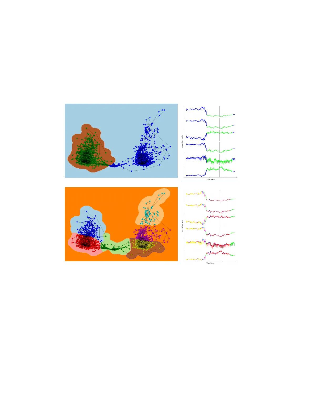
Authors: Timothy Wong, Zhiyuan Luo
Recurr ent A uto-Encoder Model f or Large-Scale Industrial Sensor Signal Analysis ? T imothy W ong [0000 − 0003 − 1943 − 6448] and Zhiyuan Luo [0000 − 0002 − 3336 − 3751] Royal Hollo way , Univ ersity of London, Egham TW20 0EX, United Kingdom. Abstract. Recurrent auto-encoder model summarises sequential data through an encoder structure into a fix ed-length vector and then reconstructs the original sequence through the decoder structure. The summarised vector can be used to represent time series features. In this paper , we propose relaxing the dimensionality of the decoder output so that it performs partial reconstruction. The fixed-length vector therefore represents features in the selected dimensions only . In addition, we propose using rolling fixed window approach to generate training samples from unbounded time series data. The change of time series features ov er time can be summarised as a smooth trajectory path. The fixed-length vectors are further analysed using additional visualisation and unsupervised clustering techniques. The proposed method can be applied in large-scale industrial processes for sensors signal analysis purpose, where clusters of the vector representations can reflect the operating states of the industrial system. Keyw ords: Recurrent Auto-encoder · Multidimensional T ime Series · Industrial Sensors · Signal Anal- ysis. 1 Background Modern industrial processes are often monitored by a large array of sensors. Machine learning techniques can be used to analyse unbounded streams of sensor signal in an on-line scenario. This paper illustrates the idea using propietary data collected from a two-stage centrifugal compression train driven by an aeroderiv ati ve industrial engine (Rolls-Royce RB211) on a single shaft. This large-scale compression module belongs to a major natural gas terminal 1 . The purpose of this modular process is to regulate the pressure of natural gas at an elev ated, pre-set level. At the compression system, sensors are installed to monitor the production process. Real-v alued measurements such as temperature, pressure, rotary speed, vibration... etc., are recorded at different locations 2 . Streams of sensor signals can be treated as a multidimensional entity changing through time. Each stream of sensor measurement is basically a set of real values receiv ed in a time-ordered fashion. When this concept is extended to a process with P sensors, the dataset can therefore be expressed as a time-ordered multidi- mensional vector { R P t : t ∈ [1 , T ] } . The dataset used in this study is unbounded (i.e. continuous streaming) and unlabelled, where the events of interest (e.g. ov erheating, mechanical failure, blocked oil filters... etc) are not present. The key goal of this study is to identify sensor patterns and anomalies to assist equiptment maintenance. This can be achieved ? Supported by Centrica plc. Registered of fice: Millstream, Maidenhead Road, W indsor SL4 5GD, United Kingdom. 1 A simplified process diagram of the compression train can be found in Figure 6 at the appendix. 2 A list of sensors is av ailable in the appendix. 2 W ong and Luo. by finding the representation of multiple sensor data. W e propose using recurrent auto-encoder model to extract vector representation for multidimensional time series data. V ectors can be analysed further using visualisation and clustering techniques in order to identify patterns. 1.1 Related W orks A comprehensive revie w [1] analysed traditional clustering algorithms for unidimensional time series data. It has concluded that Dynamic Time W arping (DTW) can be an effecti v e benchmark for unidimensional time series data representation. There has been attempts to generalise DTW to multidimensional level [20,5,8,11,15,13,21,16,6]. Most of these studies focused on analysing time series data with relativ ely low dimensionality , such as those collected from Internet of Things (IoT) devices, wearable sensors and gesture recognition. This paper contrib utes further by featuring a time series dataset with much higher dimensional- ity which is representativ e for an y large-scale industrial applications. Among neural network researches, [18] proposed a recurrent auto-encoder model based on LSTM neu- rons which aims at learning video data representation. It achiev es this by reconstructing sequence of video frames. Their model was able to deriv e meaningful representations for video clips and the reconstructed out- puts demonstrate sufficient similarity based on qualitativ e examination. Another recent paper [4] also used LSTM-based recurrent auto-encoder model for video data representation. Sequence of frames feed into the model so that it learns the intrinsic representation of the underlying video source. Areas with high recon- struction error indicate di ver gence from the kno wn source and hence can be used as a video forgery detection mechanism. Similarly , audio clips can treated as sequential data. A study [3] conv erted variable-length audio data into fixed-length vector representation using recurrent auto-encoder model. It found that audio se gments that sound alike usually ha ve v ector representations in same neighbourhood. There are other works related to time series data. For instance, a recent paper [14] proposed a recurrent auto-encoder model which aims at providing fixed-length representation for bounded univ ariate time series data. The model was trained on a plurality of labelled datasets with the aim of becoming a generic time series feature extractor . Dimensionality reduction of the vector representation via t-SNE sho ws that the ground labels can be observed in the extracted representations. Another study [9] proposed a time series compression algorithm using a pair of RNN encoder-decoder structure and an additional auto-encoder to achiev e higher compression ratio. Meanwhile, another research [12] used an auto-encoder model with database metrics (e.g. CPU usage, number of acti v e sessions... etc) to identify anomalous usage periods by setting threshold on the reconstruction error . 2 Methods A pair of RNN encoder-decoder structure can pro vide end-to-end mapping between an ordered multidimen- sional input sequence and its matching output sequence [19,2]. Recurrent auto-encoder can be depicted as a special case of the aforementioned model, where input and output sequences are aligned with each other . It can be extended to the area of signal analysis in order to lev erage recurrent neurons power to understand complex and time-dependent relationship. 2.1 Encoder -Decoder Structure At high lev el, the RNN encoder reads an input sequence and summarises all information into a fixed-length vector . The decoder then reads the vector and reconstructs the original sequence. Figure 1 below illustrates the model. Recurrent Auto-Encoder Model for Large-Scale Industrial Sensor Signal Analysis 3 Fig. 1: Recurrent auto-encoder model. Both the encoder and decoder are made up of multilayered RNN. Arrows indicate the direction of information flo w . Encoding The role of the recurrent encoder is to project the multidimensional input sequence into a fixed-length hidden context vector c . It reads the input vectors { R P t : t ∈ [1 , T ] } sequentially from t = 1 , 2 , 3 , ..., T . The hidden state of the RNN has H dimensions which updates at ev ery time step based on the current input and hidden state inherited from previous steps. Recurrent neurons arranged in multiple layers are capable of learning comple x temporal beha viours. In this proposed model, LSTM neurons with hyperbolic tangent activ ation are used at all recurrent layers [7]. An alternativ e choice of using gated recurrent unit (GR U) neurons [2] can also be used but was not experimented within the scope of this study . Once the encoder reads all the input information, the sequence is summarised in a fixed-length v ector c which has H hidden dimensions. For regularisation purpose, dropout can be applied to av oid overfitting. It refers to randomly removing a fraction of neurons during training, which aims at making the netw ork more generalisable [17]. In an RNN setting, [22] suggested that dropout should only be applied non-recurrent connections. This helps the recurrent neurons to retain memory through time while still allowing the non-recurrent connections to benefit from regularisation. Decoding The decoder is a recurrent network which uses the representation c to reconstruct the original sequence. T o ex emplify this, the decoder starts by reading the context vector c at t = 1 . It then decodes the information through the RNN structure and outputs a sequence of vectors { R K t : t ∈ [1 , T ] } where K denotes the dimensionality of the output sequence. Recalling one of the fundamental characteristics of an auto-encoder is the ability to reconstruct the input data back into itself via a pair of encoder-decoder structure. This criterion can be slightly relaxed such that K 6 P , which means the output sequence is only a partial reconstruction of the input sequence. Recurrent auto-encoder with partial reconstruction: ( f encoder : { R P t : t ∈ [1 , T ] } → c f decoder : c → { R K t : t ∈ [1 , T ] } K 6 P (1) In the large-scale industrial system use case, all streams of sensor measurements are included in the input dimensions while only a subset of sensors is included in the output dimensions. This means that the 4 W ong and Luo. entire system is visible to the encoder, but the decoder only needs to perform partial reconstruction of it. End-to-end training of the relaxed auto-encoder implies that the context vector would summarise the input sequence while still being conditioned on the output sequence. Giv en that activ ation of the context vector is conditional on the decoder output, this approach allows the encoder to capture lead variables across the entire process as long as they are rele v ant to the selected output dimensions. It is important to recognise that reconstructing part of the data is an easier task to perform than fully- reconstructing the entire original sequence. Howe ver , partial reconstruction has practical significance for industrial applications. In real-life scenarios, multiple conte xt v ectors can be generated from dif ferent recur- rent auto-encoder models using identical sensors in the encoder input but different subset of sensors in the decoder output. The selected subsets of sensors can reflect the underlying operating states of different parts of the industrial system. As a result, context vectors produced from the same temporal segment can be used as dif ferent diagnostic measurements in industrial context. W e will illustrate this in the results section by two examples. 2.2 Sampling For a training dataset of T 0 time steps, samples can be generated where T < T 0 . W e can begin at t = 1 and draw a sample of length T . This process continues recursiv ely by shifting one time step until it reaches the end of the training dataset. For a subset sequence with length T , this method allows T 0 − T samples to be generated. Besides, it can also generate samples from an unbounded time series in an on-line scenrio, which are essential for time-critical applications such as sensor data analysis. Algorithm 1: Drawing samples consecuti v ely from the original dataset Input: Dataset length T 0 Input: Sample length T 1 i ← 0 ; 2 while i 6 i + T do 3 Generate sample sequence ( i, i + T ] from the dataset; 4 i ← i + 1 ; 5 end Giv en that sample sequences are recursively generated by shifting the window by one time step, successiv ely- generated sequences are highly correlated with each other . As we hav e discussed previously , the RNN en- coder structure compresses sequential data into a fixed-length vector representation. This means that when consecutiv e sequences are fed through the encoder structure, the resulting acti v ation at c would also be highly correlated. As a result, consecutiv e conte xt vectors can join up to form a smooth trajectory in space. Context vectors in the same neighbourhood have similar activ ation therefore the industrial system must hav e similar underlying operating states. Contrarily , context vectors located in distant neighbourhoods would hav e different underlying operating states. These context vectors can be visualised in lower dimensions via dimensionality reduction techniques such as principal component analysis (PCA). Furthermore, additional unsupervised clustering algorithms can be applied to the context vectors. Each context vector can be assigned to a cluster C j where J is the total number of clusters. Once all the context vectors are labelled with their corresponding clusters, supervised classification algorithms can be used to learn the relationship between them using the training set. For instance, support vector machine (SVM) classifier with J classes can be used. The trained classifier can then be applied to the context vectors in the held-out validation set for cluster assignment. It can also be applied to context vectors generated from Recurrent Auto-Encoder Model for Large-Scale Industrial Sensor Signal Analysis 5 unbounded time series in an on-line setting. Change in cluster assignment among successive context vectors indicates a change in the underlying operating state. 3 Results T raining samples were drawn from the dataset using windowing approach with fixed sequence length. In our example, the large-scale industrial system has 158 sensors which means the recurrent auto-encoder’ s input dimension has P = 158 . Observ ations are taken at 5 minutes granularity and the total duration of each sequence was set at 3 hours. This means that the model’ s sequence has fixed length T = 36 , while samples were drawn from the dataset with total length T 0 = 2724 . The dataset was scaled into z -scores, thus ensuring zero-centred data which facilitates gradient-based training. The recurrent auto-encoder model has three layers in the RNN encoder structure and another three layers in the corresponding RNN decoder . There are 400 neurons in each layer . The auto-encoder model structure can be summarised as: RNN encoder ( 400 neurons / 3 layers LSTM / hyperbolic tangent) - Context layer ( 400 neurons / Dense / linear activ ation) - RNN decoder ( 400 neurons / 3 layers LSTM / h yperbolic tangent). Adam optimiser [10] with 0 . 4 dropout rate was used for model training. 3.1 Output Dimensionity As we discussed earlier , the RNN decoder’ s output dimension can be relaxed for partial reconstruction. The output dimensionality was set at K = 6 which is comprised of a selected set of sensors relating to key pressure measurements (e.g. suction and discharge pressures of the compressor de vice). W e have e xperimented three scenarios where the first two ha v e complete dimensionality P = 158; K = 158 and P = 6; K = 6 while the remaining scenario has relaxed dimensionality P = 158; K = 6 . The training and validation MSEs of these models are visualised in figure 2 belo w . Fig. 2: Effects of relaxing dimensionality of the output sequence on the training and validation MSE losses. They contain same number of layers in the RNN encoder and decoder respectiv ely . All hidden layers contain same number of LSTM neurons with hyperbolic tangent acti v ation. 6 W ong and Luo. The first model with complete dimensionality ( P = 158; K = 158 ) has visibility of all dimensions in both the encoder and decoder structures. Y et, both the training and validation MSEs are high as the model struggles to compress-decompress the high dimensional time series data. For the complete dimensionality model with P = 6; K = 6 , the model has limited visibility to the system as only the selected dimensions were included. Despite the context layer summarises information specific to the selected dimensionality in this case, lead variables in the original dimensions have been excluded. This prev ents the model from learning an y dependent behaviours among all a v ailable information. On the other hand, the model with partial reconstruction ( P = 158; K = 6 ) demonstrate substantially lower training and v alidation MSEs. Since all information is av ailable to the model via the RNN encoder , it captures the relev ant information such as lead variables across the entire system. Randomly selected samples in the held-out validation set were fed to this model and the predictions can be qualitatively examined in details. In figure 3 belo w , all the selected specimens demonstrate high similarity between the original label and the reconstructed output. The recurrent auto-encoder model captures the shift in mean lev el as well as temporal v ariations across all output dimensions. Fig. 3: A heatmap showing eight randomly selected output sequences in the held-out validation set. Colour represents magnitude of sensor measurements in normalised scale. 3.2 Context V ector Once the recurrent auto-encoder model is successfully trained, samples can be fed to the model and the corresponding context vectors can be extracted for detailed inspection. In the model we selected, the con- text vector c is a multi-dimensional real vector R 400 . Since the model has input dimensions P = 158 and sequence length T = 36 , the model has achie ved compression ratio 158 × 36 400 = 14 . 22 . Dimensionality reduc- Recurrent Auto-Encoder Model for Large-Scale Industrial Sensor Signal Analysis 7 tion of the context vectors through principal component analysis (PCA) shows that context vectors can be efficiently embedded in lo wer dimensions (e.g. two-dimensional space). At lo w-dimensional space, we used supervised classification algorithm to learn the relationship between vectors representations and cluster assignment. The trained classification model can then be applied to the validation set to assign clusters for unseen data. In our experiment, a SVM classifier with radial basis function (RBF) kernel ( γ = 4 ) was used. The results are shown in figure 4 belo w . (a) 2 clusters (b) 6 clusters Fig. 4: The first example. On the left, the context vectors were projected into two-dimensional space using PCA. The black solid line on the left joins all consecutiv e context vectors together as a trajectory . Different number of clusters were identified using simple K -means algorithm. Cluster assignment and the SVM deci- sion boundaries are coloured in the charts. On the right, output dimensions are visualised on a shared time axis. The black solid line demarcates the training set ( 70% ) and v alidation sets ( 30% ). The line segments are colour-coded to match the corresponding clusters. In two-dimensional space, the conte xt vectors separate into tw o clearly identifiable neighbourhoods. These two distinct neighbourhoods correspond to the shift in mean values across all output dimensions. 8 W ong and Luo. When K -means clustering algorithm is applied, it captures these two neighbourhoods as two clusters in the scenario depicted in figure 4a. When the number of clusters increases, they begin to capture more subtleties. In the six clusters scenario illustrated in figure 4b, successiv e context vectors oscillate back and forth between neighbouring clusters. The trajectory corresponds to the interlacing troughs and crests in the output dimensions. Similar pattern can also be observed in the validation set, which indicates that the kno wledge learned by the auto-encoder model is generalisable to unseen data. Furthermore, we ha ve repeated the same experiment again with a different configuration ( K = 158; P = 2 ) to reassure that the proposed approach can pro vide robust representations of the data. The sensor measure- ments are dra wn from an identical time period and only the output dimensionality K is changed (The ne wly selected set of sensors is comprised of a dif ferent measurements of dischar ge g as pressure at the compressor unit). Through changing the output dimensionality K , we can illustrate the effects of partial reconstruc- tion using different output dimensions. As seen in figure 5, the context vectors form a smooth trajectory in the low-dimensional space. Similar sequences yield context vectors which are located in a shared neigh- bourhood. Nev ertheless, the clusters found by K -means method in this secondary example also manage to identify neighbourhoods with similar sensor patterns. (a) 2 clusters (b) 6 clusters Fig. 5: The second example. The sensor data is drawn from the same time period as the previous example, only the output dimension has been changed to K = 2 where another set of gas pressure sensors were selected. Recurrent Auto-Encoder Model for Large-Scale Industrial Sensor Signal Analysis 9 4 Discussion and Conclusion Successiv e context vectors generated by windowing approach are always highly correlated, thus form a smooth trajectory in high-dimensional space. Additional dimensionality reduction techniques can be applied to visualise the change of time series features. One of the key contributions of this study is that similar context vectors can be grouped into clusters using unsupervised clustering algorithms such as K -means algorithm. Clusters can be optionally labelled manually to identify operating state (e.g. healthy vs. faulty). Alarm can be triggered when the context vector trav els beyond the boundary of a predefined neighbourhood. Clusters of the vector representation can be used by operators and engineers to aid diagnostics and maintenance. Another contribution of this study is that dimensionality of the output sequence can be relaxed. This allows the recurrent auto-encoder to perform partial reconstruction. Although it is easier for the model to reconstruct part of the original sequence, such simple improv ement allows users to define different sets of sensors of particular interest. By changing sensors in the decoder output, context vectors can be used to reflect underlying operating states of various aspects of the large-scale industrial process. This ultimately enables users to diagnose the industrial system by generating more useful insight. This proposed method essentially performs multidimensional time series clustering. W e hav e demon- strated that it can natively scale up to very high dimensionality as it is based on recurrent auto-encoder model. W e hav e applied the method to an industrial sensor dataset with P = 158 and empirically show that it can represent multidimensional time series data effecti vely . In general, this method can be further generalised to any multi-sensor multi-state processes for operating state recognition. This study established that recurrent auto-encoder model can be used to analyse unlabelled and un- bounded time series data. It further demontrated that operating state (i.e. labels) can be inferred from un- labelled time series data. This opens up further possibilities for analysing complex industrial sensors data giv en that it is predominately o verwhelmed with unbounded and unlabelled time series data. Nev ertheless, the proposed approach has not included any categorical sensor measurements (e.g. open/closed, tripped/healthy , start/stop... etc). Future research can focus on incorporating categorical measurements along- side real-valued measurements. Disclosure The technical method described in this paper is the subject of British patent application GB1717651.2. References 1. Bagnall, A., Lines, J., Bostrom, A., Large, J., Keogh, E.: The great time series classification bake of f: a revie w and experimental ev aluation of recent algorithmic advances. Data Mining and Knowledge Discov- ery 31 (3), 606–660 (May 2017). https://doi.org/10.1007/s10618-016-0483-9, https://doi.org/10.1007/ s10618- 016- 0483- 9 2. Cho, K., v an Merrienboer , B., G ¨ ulc ¸ ehre, C ¸ ., Bougares, F ., Schwenk, H., Bengio, Y .: Learning phrase representations using RNN encoder-decoder for statistical machine translation. CoRR abs/1406.1078 (2014), http://arxiv. org/abs/1406.1078 3. Chung, Y ., W u, C., Shen, C., Lee, H., Lee, L.: Audio word2vec: Unsupervised learning of audio segment represen- tations using sequence-to-sequence autoencoder. CoRR abs/1603.00982 (2016), 1603.00982 4. D’A vino, D., Cozzolino, D., Poggi, G., V erdoli va, L.: Autoencoder with recurrent neural networks for video forgery detection. CoRR abs/1708.08754 (2017), 10 W ong and Luo. 5. Gillian, N.E., Knapp, R.B., O’Modhrain, M.S.: Recognition of multivariate temporal musical gestures using n- dimensional dynamic time warping. In: NIME (2011) 6. Giorgino, T .: Computing and visualizing dynamic time warping alignments in r: The dtw package. Journal of Statis- tical Software, Articles 31 (7), 1–24 (2009). https://doi.or g/10.18637/jss.v031.i07, https://www.jstatsoft. org/v031/i07 7. Hochreiter , S., Schmidhuber , J.: Long short-term memory . Neural Computation 9 (8), 1735–1780 (Nov 1997). https://doi.org/10.1162/neco.1997.9.8.1735, http://dx.doi.org/10.1162/neco.1997.9.8.1735 8. ten Holt, G., Reinders, M., Hendriks, E.: Multi-dimensional dynamic time warping for gesture recognition (01 2007) 9. Hsu, D.: Time series compression based on adaptiv e piecewise recurrent autoencoder . CoRR abs/1707.07961 (2017), 10. Kingma, D.P ., Ba, J.: Adam: A method for stochastic optimization. CoRR abs/1412.6980 (2014), http:// 11. K o, M.H., W est, G., V enkatesh, S., Kumar , M.: Online context recognition in multisensor systems using dynamic time warping. In: 2005 International Conference on Intelligent Sensors, Sensor Networks and Information Process- ing. pp. 283–288 (Dec 2005). https://doi.org/10.1109/ISSNIP .2005.1595593 12. Lee, D.: Anomaly Detection in Multiv ariate Non-stationary Time Series for Automatic DBMS Diagnosis. ArXiv e-prints (Aug 2017) 13. Liu, J., W ang, Z., Zhong, L., W ickramasuriya, J., V asude v an, V .: uw a ve: Accelerometer -based personalized gesture recognition and its applications. In: 2009 IEEE International Conference on Pervasi v e Computing and Communi- cations. pp. 1–9 (March 2009). https://doi.org/10.1109/PERCOM.2009.4912759 14. Malhotra, P ., TV , V ., V ig, L., Agarwal, P ., Shroff, G.: Timenet: Pre-trained deep recurrent neural network for time series classification. CoRR abs/1706.08838 (2017), 15. Petitjean, F ., Inglada, J., Gancarski, P .: Satellite image time series analysis under time warping. IEEE T ransactions on Geoscience and Remote Sensing 50 (8), 3081–3095 (Aug 2012). https://doi.org/10.1109/TGRS.2011.2179050 16. Shokoohi-Y ekta, M., Hu, B., Jin, H., W ang, J., Keogh, E.: Generalizing dtw to the multi-dimensional case requires an adaptiv e approach. Data Mining and Kno wledge Discovery 31 (1), 1–31 (Jan 2017). https://doi.org/10.1007/s10618- 016-0455-0, https://doi.org/10.1007/s10618- 016- 0455- 0 17. Sriv asta v a, N., Hinton, G., Krizhe vsky , A., Sutske ver , I., Salakhutdinov , R.: Dropout: A simple w ay to prevent neural networks from overfitting. Journal of Machine Learning Research 15 , 1929–1958 (2014), http://jmlr.org/ papers/v15/srivastava14a.html 18. Sriv asta v a, N., Mansimov , E., Salakhutdinov , R.: Unsupervised learning of video representations using lstms. CoRR abs/1502.04681 (2015), 19. Sutske ver , I., V in yals, O., Le, Q.V .: Sequence to sequence learning with neural networks. CoRR abs/1409.3215 (2014), 20. Vlachos, M., Hadjieleftheriou, M., Gunopulos, D., Keogh, E.: Indexing multidimensional time-series. The VLDB Journal 15 (1), 1–20 (Jan 2006). https://doi.org/10.1007/s00778-004-0144-2, https://doi.org/10.1007/ s00778- 004- 0144- 2 21. W ang, J., Balasubramanian, A., Mojica de la V ega, L., Green, J., Samal, A., Prabhakaran, B.: W ord recognition from continuous articulatory mov ement time-series data using symbolic representations (08 2013) 22. Zaremba, W ., Sutskever , I., V inyals, O.: Recurrent neural network regularization. CoRR abs/1409.2329 (2014), Recurrent Auto-Encoder Model for Large-Scale Industrial Sensor Signal Analysis 11 A ppendix A The rotary components are driv en by industrial RB-211 jet turbine on a single shaft through a gearbox. Incoming natural gas passes through the low pressure (LP) stage first which brings it to an intermediate pressure lev el, it then passes through the high pressure (HP) stage and reaches the pre-set desired pressure lev el. The purpose of the suction scrubber is to remov e an y remaining condensate from the gas prior to feed- ing through the centrifugal compressors. Once the hot compressed gas is discharged from the compressor, its temperature is lowered via the intercoolers. Fig. 6: A simplified process diagram of the two-stage centrifugal compression train which is located at a natural gas terminal. Fig. 7: Locations of key components around the centrifug al compressor . 12 W ong and Luo. A ppendix B The sensor measurements used in the analysis are listed below: 1. GASCOMPCARBONDIO XIDEMEAS 2. GASCOMPMETHANEMEAS 3. GASCOMPNITR OGENMEAS 4. GASPR OPMOL WTMEAS 5. PRESSAMBIENT 6. GB SPEEDINPUT 7. GB SPEEDOUTPUT 8. GB TEMPINPUTBRGDRIVEEND 9. GB TEMPINPUTBRGNONDRIVEEND 10. GB TEMPINPUTBRGTHR USTINBO ARD 11. GB TEMPINPUTBRGTHR USTOUTBRD 12. GB TEMPLUBOIL 13. GB TEMPLUBOIL T ANK 14. GB TEMPOUTPUTBRGDRIVEEND 15. GB TEMPOUTPUTBRGNONDRIVEEND 16. GB VIBBRGCASINGVEL 17. GB VIBINPUT AXIALDISP 18. GB VIBINPUTDRIVEEND 19. GB VIBINPUTNONDRIVEEND 20. GB VIBOUTPUTDRIVEEND 21. GB VIBOUTPUTNONDRIVEEND 22. GG FLOWFUEL 23. GG FLOWW A TERINJECTION 24. GG FLOWW A TERINJSETPOINT 25. GG POWERSHAFT 26. GG PRESSAIRINLET 27. GG PRESSCOMPDEL 28. GG PRESSCOMPDELHP 29. GG PRESSCOMPDELIP 30. GG PRESSDIFBRGLUBOIL 31. GG PRESSDIFINLETFIL TER 32. GG PRESSDIFINLETFLARE 33. GG PRESSDIFV AL VEW A TERINJCTRL 34. GG PRESSDISCHW A TERINJPUMP1 35. GG PRESSDISCHW A TERINJPUMP2 36. GG PRESSEXH 37. GG PRESSFUELGAS 38. GG PRESSHYDOILDEL 39. GG PRESSLUBEOILHEADER 40. GG PRESSLUBOIL 41. GG PRESSMANIFOLDW A TERINJ 42. GG PRESSSUCTW A TERINJPUMP 43. GG SPEEDHP 44. GG SPEEDIP 45. GG TEMP AIRINLET 46. GG TEMPCOMPDEL 47. GG TEMPCOMPDELHP 48. GG TEMPCOMPDELIP 49. GG TEMPEXH 50. GG TEMPEXHTC1 51. GG TEMPEXHTC2 52. GG TEMPEXHTC3 53. GG TEMPEXHTC4 54. GG TEMPEXHTC5 55. GG TEMPEXHTC6 56. GG TEMPEXHTC7 57. GG TEMPEXHTC8 58. GG TEMPFUELGAS 59. GG TEMPFUELGASG1 60. GG TEMPFUELGASLINE 61. GG TEMPHSOILCOOLANTRETURN 62. GG TEMPHSOILMAINRETURN 63. GG TEMPLUBOIL 64. GG TEMPLUBOIL T ANK 65. GG TEMPPURGEMUFF 66. GG TEMPW A TERINJSUPPL Y 67. GG V AL VEW A TERINJECTCONTR OL 68. GG V ANEINLETGUIDEANGLE 69. GG V ANEINLETGUIDEANGLE1 70. GG V ANEINLETGUIDEANGLE2 71. GG VIBCENTREBRG 72. GG VIBFR ONTBRG 73. GG VIBREARBRG 74. HP HEAD ANTISURGE 75. HP POWERSHAFT 76. HP PRESSCLEANGAS 77. HP PRESSDIF ANTISURGE 78. HP PRESSDIFSUCTSTRAINER 79. HP PRESSDISCH 80. HP PRESSSEALDR YGAS 81. HP PRESSSEALLEAKPRIMAR YDE1 82. HP PRESSSEALLEAKPRIMAR YDE2 83. HP PRESSSEALLEAKPRIMAR YNDE1 84. HP PRESSSEALLEAKPRIMAR YNDE2 85. HP PRESSSUCT1 86. HP PRESSSUCT2 87. HP SPEED 88. HP TEMPBRGDRIVEEND 89. HP TEMPBRGNONDRIVEEND 90. HP TEMPBRGTHR USTINBO ARD 91. HP TEMPBRGTHR USTOUTBO ARD 92. HP TEMPDISCH1 93. HP TEMPDISCH2 94. HP TEMPLUBOIL 95. HP TEMPLUBOIL T ANK 96. HP TEMPSUCT1 97. HP VIBAXIALDISP1 98. HP VIBAXIALDISP2 99. HP VIBDRIVEEND 100. HP VIBDRIVEENDX 101. HP VIBDRIVEEND Y 102. HP VIBNONDRIVEEND 103. HP VIBNONDRIVEENDX 104. HP VIBNONDRIVEEND Y 105. HP V OLDISCH 106. HP V OLRA TIO 107. HP V OLSUCT 108. LP HEAD ANTISURGE 109. LP POWERSHAFT 110. LP PRESSCLEANGAS 111. LP PRESSDIF ANTISURGE 112. LP PRESSDIFSUCTSTRAINER 113. LP PRESSDISCH 114. LP PRESSSEALDR YGAS 115. LP PRESSSEALLEAKPRIMAR YDE1 116. LP PRESSSEALLEAKPRIMAR YDE2 117. LP PRESSSEALLEAKPRIMAR YNDE1 118. LP PRESSSEALLEAKPRIMAR YNDE2 119. LP PRESSSUCT1 120. LP PRESSSUCT2 121. LP SPEED 122. LP TEMPBRGDRIVEEND 123. LP TEMPBRGNONDRIVEEND 124. LP TEMPBRGTHR USTINBO ARD 125. LP TEMPBRGTHR USTOUTBO ARD 126. LP TEMPDISCH1 127. LP TEMPDISCH2 128. LP TEMPLUBOIL 129. LP TEMPLUBOIL T ANK 130. LP TEMPSUCT1 131. LP VIBAXIALDISP1 132. LP VIBAXIALDISP2 133. LP VIBDRIVEEND 134. LP VIBDRIVEENDX 135. LP VIBDRIVEEND Y 136. LP VIBNONDRIVEEND 137. LP VIBNONDRIVEENDX 138. LP VIBNONDRIVEEND Y 139. LP V OLDISCH 140. LP V OLRA TIO 141. LP V OLSUCT 142. PT POWERSHAFT 143. PT SPEED 144. PT TEMPBRGDRIVEEND 145. PT TEMPBRGNONDRIVEEND 146. PT TEMPBRGTHR UST1 147. PT TEMPBRGTHR UST3 148. PT TEMPCOOLINGAIR1 149. PT TEMPCOOLINGAIR2 150. PT TEMPEXH 151. PT TEMPLUBOIL 152. PT TEMPLUBOILPTSUMP 153. PT TEMPLUBOIL T ANK 154. PT VIBAXIALDISP1 155. PT VIBAXIALDISP2 156. PT VIBBRGCASINGVEL 157. PT VIBDRIVEEND 158. PT VIBNONDRIVEEND
Original Paper
Loading high-quality paper...
Comments & Academic Discussion
Loading comments...
Leave a Comment