Blind Network Revenue Management and Bandits with Knapsacks under Limited Switches

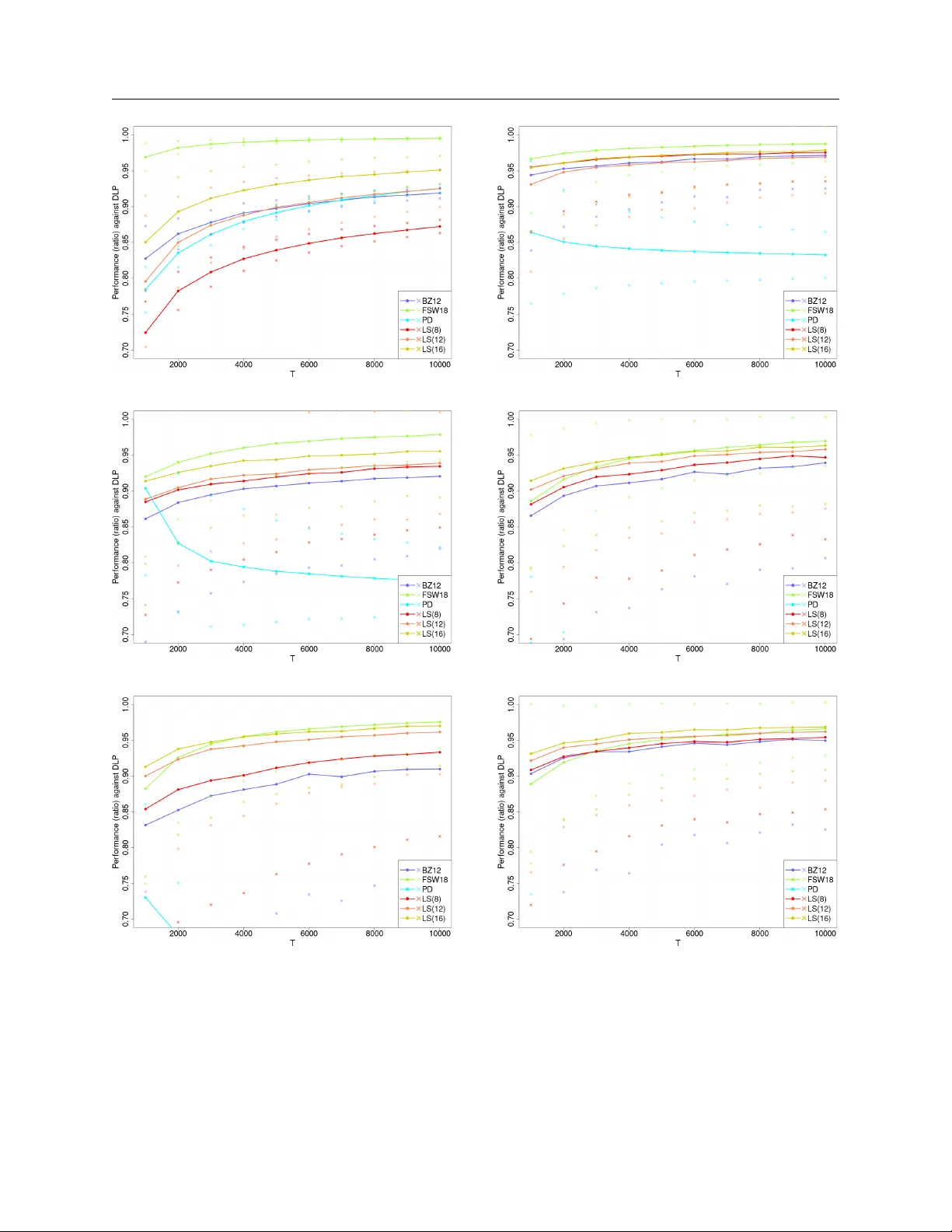
Blind Net w ork Rev en ue Managemen t and Bandits with Knapsac ks Under Limited Switc hes Da vid Simc hi-Levi Department of Civil and Environmental Engineering, Operations Research Center, and Institute for Data, Systems, and Society , Massachusetts Institute of T echnology , Cam bridge, MA 02139, dslevi@mit.edu Y unzong Xu Department of Industrial and Enterprise Systems Engineering, Grainger College of Engineering, Univ ersit y of Illinois, Urbana-Champaign, IL 61801, xyz@illinois.edu Jinglong Zhao Questrom School of Business, Boston Universit y , Boston, MA, 02215, jinglong@bu.edu This paper studies the impact of limited switches on resource-constrained dynamic pricing with demand learning. W e fo cus on the classical price-based blind netw ork reven ue management problem and extend our results to the bandits with knapsacks problem. In b oth settings, a decision maker faces sto c hastic and distri- butionally unkno wn demand, and m ust allo cate ﬁnite initial in ven tory across m ultiple resources o v er time. In addition to standard resource constraints, we impose a switching constraint that limits the num b er of action c hanges o ver the time horizon. W e establish matching upper and lo wer bounds on the optimal regret and dev elop computationally eﬃcient limited-switc h algorithms that achiev e it. W e show that the optimal regret rate is fully characterized by a piecewise-constan t function of the switching budget, whic h further dep ends on the num b er of resource constraints. Our results highlight the fundamental role of resource constraints in shaping the statistical complexit y of online learning under limited switches. Extensiv e simulations demon- strate that our algorithms main tain strong cum ulative reward p erformance while signiﬁcan tly reducing the n umber of switches. Key words : net work reven ue management, bandits with knapsacks, online learning, limited switches 1. Intro duction In this pap er, w e consider the classical price-based blind netw ork rev enue managemen t ( BNRM ) problem ( Besb es and Zeevi 2012 ) and its extension to the bandits with knapsac ks ( BwK ) problem ( Badanidiyuru et al. 2013 ). In the BNRM problem, a ﬁrm is endow ed with some ﬁnite inv entory of m ultiple resources to sell ov er a ﬁnite time horizon. The starting in ven tory is unreplenishable and exogenously given. The ﬁrm can con trol its sales through sequen tial decisions on the prices oﬀered. The ﬁrm’s ob jectiv e is to maximize its exp ected cumulativ e reven ue. 1 2 W e consider the setup in which demand is stochastic, indep enden t and time-homogeneous. Y et the distributional information is unknown to the ﬁrm, and has to b e sequentially learned ov er the selling horizon. In such a setup, any optimal policy m ust instan taneously adjust its prices and switc h b et ween the prices in real time ( Badanidiyuru et al. 2013 , Besbes and Zeevi 2012 , F erreira et al. 2018 ). Ho wev er, not all ﬁrms ha ve the infrastructure to query the realized demand in real time, to adjust their decisions instantaneously , or to switc h b etw een the prices as freely as p ossible. Chang- ing the p osted prices is costly for man y ﬁrms ( Bray and Stamatop oulos 2022 , Levy et al. 1998 , Stamatop oulos et al. 2020 , Zbarac ki et al. 2004 ), and frequen t price changes ma y confuse the cus- tomers ( Jørgensen et al. 2003 ). A common practice for man y ﬁrms is to restrict the n um b er of price c hanges to be within a budgeted n um b er ( Chen et al. 2015 , 2020 , Cheung et al. 2017 , Netessine 2006 , Perakis and Singhvi 2023 , Simc hi-Levi and Xu 2023 ). Motiv ated by this c hallenge, we analyze the impact of limited switches on the classical blind net work rev en ue managemen t ( BNRM ) problem. W e incorporate an additional constrain t of limited switc hing budget into the classical BNRM mo del and form ulate a new problem: blind netw ork rev enue management under limited switc hes ( BNRM-LS ). F or the BNRM-LS problem, we establish tigh t upp er and low er b ounds on the optimal regret, and design limited-switch algorithms that ac hieve the optimal regret rate. Our results c haracterize the optimal regret rate as a function of the switching budget, which further dep ends on the num b er of resources. Additionally , we consider the more general bandits with knapsac ks ( BwK ) problem ( Badani- diyuru et al. 2013 , Slivkins and V aughan 2014 ). The BwK problem generalizes the BNRM problem in the sense that rew ards (rev en ue) and costs (consumption of resources) can ha v e an y arbitrary relationship, that is, they are not necessarily connected through demand v ariables. Similar to how w e formulate the blind netw ork reven ue management under limited switc hes ( BNRM-LS ) prob- lem, we form ulate the bandits with knapsac ks under limited switc hes ( BwK-LS ) problem, which extends the classical bandits with knapsacks ( BwK ) problem; see Sections EC.3 – EC.5 in the Online App endix. 1.1. Contributions This pap er app ears to b e one of the ﬁrst pap ers to study online learning problems with b oth resource and switching constraints. W e fully characterize the statistical complexit y of the BNRM- LS problem (as well as the generalization to the BwK-LS problem in the Online App endix), and pro vide optimal algorithms to solve the BNRM-LS problem. W e sho w matc hing upp er and lo w er b ounds on the optimal regret, and design nov el limited-switch algorithms to achiev e such regret. W e adopt Landau notations and use O, Ω , Θ to hide constant factors, and use e O , e Ω , e Θ to hide both 3 Figure 1 Optimal regret rate exponent lim T →∞ log R ∗ ( T ) / log T as a function of switc hing budget s in the BNRM- LS problem. Here R ∗ ( T ) stands for the optimal (i.e., minimax) regret. constan t and logarithmic factors. F or any positive real n umber x ∈ R + , w e use ⌊ x ⌋ for the largest in teger that is smaller or equal to x ; for an y non-positive real n um b er x ∈ R \ R + , we write ⌊ x ⌋ = 0. Using the ab o ve notations, our main results can b e summarized as follo ws. First, w e pro vide a computationally eﬃcien t limited-switc h algorithm and sho w that the regret is upp er b ounded b y e O  T 1 2 − 2 − ν ( s,d )  , where ν ( s, d ) = j s − d − 1 K − 1 k . Here s stands for the switc hing budget, d the n um b er of resources, and K the n umber of price v ectors in the BNRM-LS setup (the num b er of arms in the BwK-LS setup). Second, w e pro vide matc hing low er bounds (i.e., imp ossibilit y results) on the optimal regret. Sp eciﬁcally , for an y algorithm with switc hing budget s , we construct a class of BNRM instances such that the algorithm m ust incur e Ω  T 1 2 − 2 − ν ( s,d )  exp ected rev en ue loss on one of these instances. Combining the ab o ve upp er and low er b ounds, w e sho w that the optimal regret is on the order of e Θ  T 1 2 − 2 − ν ( s,d )  . Our results sho w that the optimal regret rate is completely c haracterized b y a piece-wise constan t function of the switching budget s , which further dep ends on the n umber of resources d . See Figure 1 for an illustration. Our results ha ve tw o implications. First, a total num b er of Θ(log log T ) switching budget is necessary and suﬃcien t to achiev e the optimal e Θ( √ T ) regret for the classical BNRM problem (and BwK problem as w ell). Compared with existing optimal algorithms for BNRM that would incur an Ω( T ) switching cost in the w orst case, our algorithm ac hiev es a doubly exp onential (and b est p ossible) improv emen t in the switc hing cost. Second, our results rev eal a separation on the optimal regret betw een the resource-constrained problem ( BNRM ) and the resource-unconstrained problem ( MAB ). Under the standard regime, prior literature has shown that b oth MAB and BNRM hav e the same optimal regret rate e Θ( √ T ). Our pap er sho ws that when there is a switc hing budget, the resource-constrained problem ( BNRM ) 4 exhibits a larger regret rate than the resource-unconstrained problem ( MAB ). W e explicitly char- acterize ho w the optimal regret rate depends on the n umber of resource constrain ts. If we ﬁx all the other problem primitives unc hanged and only add in one more resource constrain t, then the regret b ound is going to b e larger, illustrating that resource constrain ts indeed increase the regret — they mak e the problem “harder.” In addition, we conduct exp erimen ts to examine the p erformance of our algorithms on a numer- ical setup that is widely used in the literature 1 . Compared with b enchmark algorithms from the literature ( Besbes and Zeevi 2012 , Badanidiyuru et al. 2013 , F erreira et al. 2018 ), our prop osed algo- rithms ac hieve promising p erformance with clear adv an tages on the num b er of incurred switc hes. Our numerical results also provide practical suggestions to ﬁrms on how to design their switching budgets. 1.2. Challenges and App roaches 1.2.1. Algorithmic techniques. It is the co-existence of b oth resource and switching con- strain ts that mak e our problems particularly challenging. Indeed, when there is no resource con- strain t, the topic of switc hing cost has b een w ell-studied in the online learning literature (for b oth limited and unlimited switching budgets setups); see Agraw al et al. ( 1988 , 1990 ), Cesa-Bianchi et al. ( 2013 ), Chen and Chao ( 2019 ), Chen et al. ( 2020 ), Cheung et al. ( 2017 ), Dong et al. ( 2020 ), Guha and Munagala ( 2009 ), Perakis and Singh vi ( 2023 ), Simchi-Levi and Xu ( 2023 ) for v arious mo dels and results. In particular, prior literature has established an “ep o c h-based elimination + uniform exploration” strategy (see, e.g., P erchet et al. 2016 , Gao et al. 2019 ) which enables researc hers to design optimal algorithms for MAB with switching constraints ( Simchi-Levi and Xu 2023 ). The “ep o ch-based elimination + uniform exploration” strategy divides the time horizon in to multiple pre-determined ep o chs; at each epo ch, th e algorithm constructs conﬁdence b ounds for (the expected rew ard of ) each action, eliminates actions that are ob viously sub-optimal, and then uniformly explores each remaining action for an equal n umber of p erio ds. Ho wev er, the ab o ve strategy could easily fail in BNRM , as tw o core ideas of the ab ov e strategy , namely “eliminating individual actions” and “uniform exploration”, could result in substantial (i.e., linear) regret in BNRM . First, eliminating individual actions is a bad idea in BNRM . In BNRM , due to resource constraints, an action’s “earning p o wer” dep ends not only on its own reward and resource consumption pattern but also on the reward and resource consumption patterns of other actions that could b e eﬀectiv ely com bined with it. F or example, tw o actions that each hea vily exhaust resources 1 and 2 resp ectively ma y b e considered “bad” if used individually . Ho wev er, 1 The setup is a BNRM setup without any switching constraint. W e note that when there is a switc hing constraint, most existing algorithms would incur Ω( T ) regret, and our algorithms should obviously b e the b est choice. 5 com bining the tw o actions prop ortionally could b e optimal and generate signiﬁcantly higher total rev enue than any single action. Therefore, an y eﬀectiv e algorithm must decide on action c ombina- tions rather than individual actions; see App endix EC.2.3 for a concrete example of the failure of eliminating individual actions. Given that the space of action combinations is exp onen tially large, this p oses unique statistical and computational c hallenges for our problem. Second, unlik e in MAB , uniform exploration ov er actions is not a goo d idea in BNRM . Due to the existence of resource constrain ts, it could b e necessary for any eﬀective algorithm to com bine diﬀeren t actions in a non-uniform manner in the long term — the optimal prop ortion of each action could depend on the characteristics of all actions and has to be learned ov er time. The idea of “choosing actions uniformly” from Simc hi-Levi and Xu ( 2023 ) could result in substantial (i.e., linear) regret in BNRM ; see App endix EC.2.3 for a concrete example. T o address the t wo challenges described abov e, w e dev elop a nov el “t wo-stage linear program- ming” ( 2SLP ) approac h in Section 4.1 , which provides guidance on how to conduct eﬃcient elim- ination and exploration in BNRM . This approac h has tw o features. First, the elimination and exploration is conduced ov er action c ombinations rather than individual actions. Second, the com- plicated optimization tasks in v olved in computing the elimination and exploration strategies are reduced to solving ( K + 1) simple linear programs in t wo stages. Since the 2SLP approach is com- putationally eﬃcient, easy to mo dify , and provides a p o werful generalization of the w ell-known successive elimination principle from MAB to BNRM , we b eliev e this approach is of indep endent in terest and will b e useful in eﬃcien tly solving more complex resource-constrained online learning problems. It is worth mentioning that, without developing 2SLP as a new algorithmic principle, it is not apparen t whether one can directly mo dify existing BNRM and BwK algorithms to obtain eﬃcient limited-switc h algorithms. Note that Badanidiyuru et al. ( 2013 ) and Immorlica et al. ( 2019 ) design computationally eﬃcien t algorithms for BwK using adv ersarial online learning subroutines, whic h do es not seem to work for our purp ose as adv ersarial online learning is shown to require frequent switc hes ( Dekel et al. 2014 , Altsch uler and T alwar 2018 ). Note also that by incorp orating the dela yed update tec hniques ( Auer et al. 2002 ) in to the UCB-type algorithms ( Agra w al and Dev anur 2014 ), one ma y design a mo diﬁed UCB-type algorithm that ac hiev es e Θ( √ T ) regret using O (log T ) switc hes. This guarantee is exp onentially worse than our guarantee, as our algorithm achiev es e Θ( √ T ) regret using only O (log log T ) switc hes. 1.2.2. Lo wer b ound tec hniques. Our low er bound pro of builds on the “tracking the co ver time” argumen t of Simchi-Levi and Xu ( 2023 ), who establish regret lo w er b ounds for MAB with a single switc hing constrain t b y trac king a series of ordered stopping times and constructing hard 6 MAB instances based on (algorithm-dep enden t) realizations of the stopping times. Extending the argumen t of Simc hi-Levi and Xu ( 2023 ) from their resource-unconstrained setting to the resource- constrained setting of BNRM-LS is non-trivial, due to the follo wing t w o reasons. First, the argument of Simchi-Levi and Xu ( 2023 ) critically utilizes the fact that the regret is measured against a single ﬁxed action, but in BNRM-LS the regret is measured against a complex dynamic p olicy (which itself requires switches). Second, the analysis of Simc hi-Levi and Xu ( 2023 ) is not sensitiv e to the n umber of resource constraints d at all, but in order to match the upp er b ound of BNRM-LS , we need to establish a strengthened lo w er bound that gradually increases with d . W e address the abov e t wo challenges by developing an LP-based analysis framework to construct hard BNRM instances with specially-designed resource constrain ts and demand structures, and measuring sev eral rev en ue gaps based on clean even t analysis of the demand realization pro cess. It is w orth men tioning that no prior work in BNRM and BwK has tried to construct hard instances that in volv e multiple ( > 1) resource constraints 2 . Moreo ver, prior lo wer bound constructions that in volv e a single resource constraint ( Badanidiyuru et al. 2013 , Sank araraman and Slivkins 2020 ) are all in the BwK setup instead of the BNRM setup. Since BwK is more general than BNRM , constructing low er b ound examples for BNRM is more c hallenging than for BwK . All prior con- structions break the sp eciﬁc reward-cost structure of BNRM , th us failing to provide low er b ounds for BNRM . Compared with prior work, our lo wer b ound instance construction is considerably more complicated, as w e ha ve to deal with d resource constrain ts and w e do not w ant to break the BNRM structure. Roadmap. In Section 2 w e start with the classical discrete price BNRM mo del and then intro- duce its limited switching budget v arian t BNRM-LS . In Section 3 w e in troduce the deterministic linear program, and presen t the results in the (simple) distributionally-kno wn case. While the tec h- niques and results are standard, they build intuitions for our main results. In Section 4 w e in tro duce our main results in the distributionally-unknown case. W e pro v e matching upper and low er b ounds on the optimal regret and pro vide optimal and eﬃcien t algorithms that achiev e the optimal regret. In Section 5 w e conduct an extensive sim ulation study . In Section 6 we extend our results to the con tinuous price setting by assuming that the demand is linear. W e conclude the pap er in Sec- tion 7 . All the generalizations to the BwK-LS problem are deferred to Sections EC.3 – EC.5 in the App endix. 2 One reason is that using zero or one resource constraint is already enough for their purp oses. 7 2. Problem F ormulation W e introduce the blind netw ork rev enue managemen t ( BNRM ) mo del, and defer the bandits with knapsac ks ( BwK ) mo del to Section EC.3 in the Online App endix. The BNRM problem is a learn- ing v ersion of the classical price-based net work rev en ue managemen t ( NRM ) problem. The NRM problem is a distributionally-kno wn sto chastic con trol problem whic h originates from the airline industry ( Gallego and V an Ryzin 1997 , T alluri and V an Ryzin 1998 ), and has been extensiv ely stud- ied in the rev enue managemen t literature with div erse applications ( Adelman 2007 , Jasin 2014 , Ma et al. 2020 , T opaloglu 2009 ). The BNRM problem extends the classical NRM problem by assuming that the demand distribution is unknown and has to b e sequentially learned ov er time. The NRM problem and the BNRM problem ha ve t wo distinct setups: a discrete price setup and a contin uous price setup. In Sections 2 – 5 , we fo cus on the discrete price setup. In Section 6 w e extend to the con tinuous price setup when demand is linear. W e refer to P erakis and Singh vi ( 2023 ), Miao and W ang ( 2021 ) for more discussions of the con tinuous price setup when demand is general. BNRM setup. Let N , R and R + b e the set of positive in tegers, real n umbers and non-negativ e real n umbers, resp ectively . F or an y n ∈ N , deﬁne [ n ] = { 1 , 2 , ..., n } . Let th ere b e a discrete, ﬁnite time horizon with T p erio ds. Time starts from p erio d 1 and ends in p erio d T . Let there b e n diﬀeren t products generated by d diﬀeren t resources. Eac h resource is endo w ed with ﬁnite initial in ven tory B i , ∀ i ∈ [ d ], and B min = min i ∈ [ d ] B i . Let A = ( a ij ) i ∈ [ d ] ,j ∈ [ n ] b e the consumption matrix. Eac h entry a ij ∈ R + stands for the amoun t of inv en tory i ∈ [ d ] consumed, if one unit of pro duct j ∈ [ n ] is sold. Let A i denote the i -th row of A . Let a max = max i,j a ij b e a b ounded constant. In each perio d t , a decision mak er can p ost prices for the n pro ducts by selecting a price v ector from a ﬁnite set of K price vectors P := { p 1 , ..., p K } , which we denote using z t ∈ { p 1 , ..., p K } . A price vector is p k = ( p 1 ,k , ..., p n,k ), and p j,k ∈ [0 , p max ] is the price for pro duct j under p k . This captures situations where the prices of all the products m ust choose from a menu of price points that ha ve b een pre-determined b y mark et standards, e.g., a common men u of prices that end in $ 9.99: $ 59.99, $ 69.99, $ 79.99, $ 89.99. In online fashion retailing, the n umber of feasible price v ectors K is usually a small n um b er relativ e to the n umber of pro ducts n . Price ordering constrain ts, such as the pro duct with basic features m ust b e cheaper than the premium pro duct, signiﬁcantly reduce the n umber of price vectors to c ho ose from ( F erreira et al. 2016 ). In the ab o ve example of 4 prices in a menu, if there are 3 products that m ust satisfy a price ordering, there are only 4 feasible price v ectors to c ho ose from, which is signiﬁcantly smaller than 4 3 = 64, the n umber of feasible price v ectors without such price ordering constraints. 8 Giv en price vector p k , the demand for eac h pro duct j ∈ [ n ] is an unknown but b ounded random v ariable 3 , Q j,k := Q j ( p k ) ∈ [0 , 1], which has to b e sequentially learned o ver time. Let q j,k := E [ Q j,k ] denote the unknown mean demand for pro duct j under price p k , and we collect Q = ( Q j,k ) j ∈ [ n ] ,k ∈ [ K ] , q = ( q j,k ) j ∈ [ n ] ,k ∈ [ K ] . F or eac h unit of demand generated for product j ∈ [ n ] under price v ector p k , the decision mak er generates p j,k rev enue by depleting a ij units of each in v entory i ∈ [ d ]. If no demand is generated, all the remaining in ven tory is carried ov er to the next p eriod. The selling pro cess stops immediately when the total cum ulative demand of any resource exceeds its initial in v entory; see Section EC.3.2.1 for discussions of alternativ e stopping rules. W e use I = ( T , B , K, d, n, P , A ; Q ) to stand for a BNRM problem instance. The ob jec tiv e of the decision maker is to maximize the expected total cumulativ e rev enue o ver T p eriods. The p erformance is measured by r e gr et , whic h is deﬁned as the w orst-case exp ected rev en ue loss compared with a clairv oy an t decision mak er who is endo wed with inﬁnite switc hing budget and kno ws the true demand distributions but not the realizations. The reven ue maximization problem is equiv alen t to a regret minimization problem. Regime for regret analysis. W e deriv e non-asymptotic b ounds on the regret of policies in terms of the n umber of time p eriods T . F or all of our results (except Theorem 1 , whic h uses a linear scaling regime), w e adopt the follo wing regret analysis regime: there exists an arbitrary constan t b > 0, such that B min ≥ bT . In other words, we do not assume any sp eciﬁc form of dep endence b et ween T and B . W e only require that inv en tory is not to o scarce compared to the time horizon. This regime generalizes the standard linear scaling regime in the netw ork rev enue management literature; see, e.g., Besb es and Zeevi ( 2012 ), Bumpensanti and W ang ( 2020 ), Chen et al. ( 2019 ), Chen and Shi ( 2019 ), F erreira et al. ( 2018 ), Gallego and V an Ryzin ( 1997 ), Jasin ( 2014 ), Liu and V an Ryzin ( 2008 ), Sun et al. ( 2020 ). F ollo wing the literature, w e assume p max , a max are all constan ts that do not dep end on T or B . The other parameters K , d , and n do not dep end on T or B , either. Y et we write out our regret b ounds’ exact dep endence on K , d and n in our theorems for b etter managerial insigh ts. Obtaining regret upper and lo w er bounds that are tigh t on the orders of K , d and n is an interesting future direction. F or ease of presen tation, we also assume that d < min { n, K } − 1. Note that this assumption is only for the purp ose of a voiding rep eatedly using the notation min { d, n − 1 , K − 1 } ; all our results readily extend to the general case without assuming d < min { n, K } − 1 b y replacing d with min { d, n − 1 , K − 1 } and replacing ν ( s, d ) with j s − min { d,n − 1 ,K − 1 }− 1 { min { d,n − 1 } d + 1 , n ≥ 1 , ther e is an asso ciate d Λ numb er (deﬁne d in Se ction 3.1 ), such that any p olicy π ∈ Π[ Λ − 2] e arns an exp e cte d r evenue: Rev ( π ) ≤ J DLP − c · T , wher e c > 0 is some distribution-dep endent c onstant that p ossibly dep ends on b but do es not dep end on T . As a direct implication of Theorem 1 , we combine the inequality in Theorem 1 with the known fact that Rev ( π ∗ [ ∞ ]) ≥ J DLP − O ( √ T ) and ha v e Rev ( π ) ≤ Rev ( π ∗ [ ∞ ]) − Ω( T ). That is, the regret scales linearly with ( T , B ) when other parameters are ﬁxed. Note that, only Theorem 1 requires this linear scaling regime; all the other theorems in this paper are describ ed under a more general asymptotic regime (see discussions in Section 2 ). The lo w er b ound established in Theorem 1 holds for any Q . Suc h a result is m uch stronger than the w orst-case type low er b ounds (which tak es the worst case ov er Q ) that are widely considered in the rev enue management literature. W e outline three k ey steps here and defer the details of our proof to App endix EC.6 . W e ﬁrst iden tify a clean even t, suc h that the realized demands are close to the exp ected demands that the LP suggests. This clean even t happ ens with high probability (1 − 2 T 3 ). Second, conditioning on suc h an even t, the maxim um amount of reven ue we generate is no more than O ( √ T ) compared to what the LP suggests; and the minim um amoun t of in ven tory demanded is no less than O ( √ T ) compared to what the LP suggests, resulting in no more than O ( √ T ) of realized rev enue. In the 12 third step, w e sho w that the regret from insuﬃcient price changes scales on the order of Ω( T ), whic h dominates the O ( √ T ) amount rev enue due to randomness. S uch clean ev ent analysis, originating from the online learning literature to prov e upp er b ounds ( Badanidiyuru et al. 2013 , Slivkins 2019 , Lattimore and Szepesv´ ari 2020 ), w as recently used in Arlotto and Gurvich ( 2019 ) to pro v e lo w er b ounds. 3.3. Upp er Bounds In this section we show that when the switching budget is greater or equal to Λ − 1, then the regret is e O ( √ T ). Suc h a sub-linear guaran tee is achiev ed by t w eaking the w ell-known static con trol p olicy in the netw ork reven ue management literature ( Gallego and V an Ryzin 1997 , Co op er 2002 , Maglaras and Meissner 2006 , Liu and V an Ryzin 2008 , Ahn et al. 2019 ). W e tw eak the static con trol p olicy , so that with high probabilit y the selling horizon nev er stops earlier than the last p eriod T . See Algorithm 1 below. This is achiev ed b y selecting the v alue of γ in the ﬁrst step of Algorithm 1 . Similar ideas ha v e been used in Ha jiagha yi et al. ( 2007 ), Ma et al. ( 2021 ), Balseiro et al. ( 2019 ) to pro ve asymptotic results in diﬀeren t setups. Algorithm 1 Tw eak ed LP Policy for the NRM Problem Input: I = ( T , B , K, d, n, P, A ; Q ). P olicy: 1: Deﬁne γ = max  1 − 2 a max B min √ nT log T , 0  . 2: Solv e the DLP as deﬁned b y ( 1 ), ( 2 ), ( 3 ), and ( 4 ). Find an optimal solution with the least n um- b er of non-zero v ariables, x ∗ ∈ X . W e assume that x ∗ k , ∀ k ∈ [ K ] are in tegers, b ecause rounding issues incur a regret of at most ( d · max k p ⊤ k · q k ), which is negligible compared with √ T . 3: Arbitrarily choose any permutation σ : [ Λ ] → Z ( x ∗ ) from all ( Λ )! p ossibilities. 4: Execute: Set the price v ector to b e p σ (1) for the ﬁrst γ · x ∗ σ (1) p eriods, then p σ (2) for the next γ · x ∗ σ (2) p eriods, ..., and ﬁnally p σ ( Λ ) for the last T − γ · P Λ − 1 l =1 x ∗ σ ( l ) p eriods. W e explain the third step p erm utation. Supp ose Z ( x ∗ ) = { 1 , 3 , 4 } . In this case, Λ = 3 and there are 6 p erm utations. There are 6 p ossible p olicies as suggested in Algorithm 1 . While some of these p olicies may ha ve b etter p erformance than others, they all ac hieve e O ( √ T ) regret. Theorem 2. L et b > 0 b e an arbitr ary c onstant. F or any NRM instanc e I = ( T , B , K, d, n, P , A ; Q ) with T ≥ 1 , d ≥ 0 , K > d + 1 and B min /T ≥ b , any p olicy π as deﬁne d in Algorithm 1 satisﬁes π ∈ Π[ Λ − 1] and e arns an exp e cte d r evenue: Rev ( π ) ≥ J DLP − max { c/b, c ′ d } √ n 3 p T log T ≥ Rev ( π ∗ [ ∞ ]) − max { c/b, c ′ d } √ n 3 p T log T 13 wher e c, c ′ > 0 ar e some absolute c onstants c ompletely determine d by a max , p max . As w e will see in Section 4 , since the loss from an unkno wn distribution is on the order of e O ( √ T ), the e O ( √ T ) regret from Algorithm 1 suﬃces to serv e as a sub-routine in the last ep o c h of the main algorithm. Ev en though there are man y adv anced techniques that impro ve the e O ( √ T ) result, they are b eyond the scop e of this pap er. 4. Blind Net wo rk Revenue Management under Limited Switches In this section, we study the BNRM-LS problem, introduce an eﬃcient algorithm, and provide matc hing upp er and lo wer b ounds of the optimal regret. W e start with some deﬁnitions. Learning p olicies and clairvo y an t p olicies. In this section, we distinguish b et ween a BNRM instanc e I = ( T , B , K , d, n, P , A ; Q ) and a BNRM pr oblem P = ( T , B , K, d, n, P , A ) based on whether the underlying demand distributions Q are sp eciﬁed or not. Consider a BNRM problem P = ( T , B , K , d, n, P , A ). Let ϕ denote any non-an ticipating learning p olicy; speciﬁcally , ϕ consists of a sequence of (pos sibly randomized) decision rules ( ϕ t ) t ∈ [ T ] , where eac h ϕ t establishes a proba- bilit y k ernel mapping from the space of historical actions and observ ations in perio ds 1 , . . . , t − 1 to the space of actions at p erio d t . F or an y s ∈ N , let Φ[ s ] b e the set of learning p olicies that c hange price v ectors for no more than s times almost surely under all possible demand distributions Q . F or an y s, s ′ ∈ N such that s ≤ s ′ , Φ[ s ] ⊆ Φ[ s ′ ]. Let Φ[ ∞ ] be the set of all admissible learning policies. Let Rev Q ( ϕ ) b e the exp ected rev enue that a learning policy ϕ generates under demand distribution Q . As we ha ve deﬁned in Section 2 , π refers to a clairvoyant p olicy endow ed with full distributional information ab out the distributions Q . F or any s ∈ N , let Π Q [ s ] b e the set of clairv oy an t policies that c hange price vectors for no more than s times under the true distributions Q . F or an y s, s ′ ∈ N suc h that s ≤ s ′ , Π Q [ s ] ⊆ Π Q [ s ′ ]. Let Π Q [ ∞ ] b e the set of all admissible clairvo y ant policies. Let Rev Q ( π ) be the exp ected rev en ue that a clairv o yan t policy π ∈ Π Q generates under distributions Q . Let π ∗ Q [ s ] ∈ arg sup π ∈ Π Q [ s ] Rev ( π ) b e one optimal clairvo y ant p olicy with switc hing budget s , and π ∗ Q b e one of the optimal dynamic p olicies with an inﬁnite switc hing budget (i.e., without a switc hing constrain t). P erformance metrics. The p erformance of an s -switch learning p olicy ϕ ∈ Φ[ s ] is measured against the p erformance of the optimal s -switc h clairvo yan t p olicy π ∗ Q [ s ]. Speciﬁcally , for any BNRM problem P and switc hing budget s , w e deﬁne the s -switch r e gr et of a learning p olicy ϕ ∈ Φ[ s ] as the w orst-case diﬀerence b et ween the exp ected reven ue of the optimal s -switc h clairvo y ant p olicy π ∗ Q [ s ] and the exp ected rev enue of p olicy ϕ : R ϕ s ( T ) = sup Q  Rev Q ( π ∗ Q [ s ]) − Rev Q ( ϕ )  . 14 W e also measure the p erformance of policy ϕ against the p erformance of the optimal unlimited- switc h clairv o yan t p olicy π ∗ Q . Sp eciﬁcally , w e deﬁne the over al l r e gr et of a learning policy ϕ ∈ Φ[ s ] as the w orst-case diﬀerence b etw een the expected rev en ue of clairvo y ant policy π ∗ Q without a switc hing constrain t and the exp ected reven ue of the p olicy ϕ : R ϕ ( T ) = sup Q  Rev Q ( π ∗ Q ) − Rev Q ( ϕ )  . In tuitively , the s -switc h regret R ϕ s ( T ) measures the “informational rev enue loss” due to not kno wing the demand distributions, while the ov erall regret R ϕ ( T ) measures the “o v erall reven ue loss” due to not kno wing the demand distributions and not being able to switc h freely . Clearly , the ov erall regret R ϕ ( T ) is alw ays larger than the s -switch regret R ϕ s ( T ). In terestingly , as we will sho w later, for all s , R ϕ ( T ) and R ϕ s ( T ) are alwa ys on the same order in terms of dep endence on T . 4.1. Upp er Bounds W e prop ose a computationally eﬃcien t algorithm that provides an upp er b ound on b oth the s - switc h regret and the o v erall regret. Our algorithm, called Limite d-Switch L e arning via Two-Stage Line ar Pr o gr amming ( LS-2SLP ), is describ ed in Algorithm 2 . In Algorithm 2 and onw ards, for any v ector x ∈ R K and any k ∈ [ K ], let ( x ) k b e the k th elemen t of vector x . The design of our algorithm builds on the SS-SE algorithm prop osed in Simchi-Levi and Xu ( 2023 ), the Balanced Explo ration algorithm proposed in Badanidiyuru et al. ( 2013 ), and the Tweak ed LP policy deﬁned in Algorithm 1 . T o address the fundamen tal c hallenges inherent in our problems (as illustrated in Section 1.2 ), w e go b ey ond the ab o ve algorithms and dev elop no vel ingredien ts for eﬃcien t exploration and exploitation under both resource and switching constraints. W e provide more details b elo w. 4.1.1. Description of the algorithm. Our algorithm runs in an ep o c h schedule whic h impro ves the ep o c h schedule of the SS-SE algorithm ( Simc hi-Levi and Xu 2023 ). Sp eciﬁcally , our LS-2SLP algorithm ﬁrst computes an index ν ( s, d ) based on the switching budget s , the num b er of actions K , and the n umber of resource constraints d , then computes a series of ﬁxed time p oints { t l } ν ( s,d )+1 l =1 according to formula ( 5 ) (see also Perc het et al. 2016 , Gao et al. 2019 for the use of such form ulas in MAB ), whic h pro vides guidance on how to divide the T selling p erio ds into ν ( s, d ) + 1 ep o chs. Compared with the SS-SE algorithm which directly uses the pre-determined sequence { t l } ν ( s,d )+1 l =1 as its ep o c h schedule, our algorithm exhibits t wo notable diﬀerences in deter- mining the epo ch sc hedule. First, the parameter ν ( s, d ) takes account of the n um b er of resource constrain ts d . Second, our algorithm uses an adaptive ep o c h sc hedule { T l } ν ( s,d )+1 l =1 rather than the pre-determined sc hedule { t l } ν ( s,d )+1 l =1 — in particular, our algorithm decides the length of the next 15 Algorithm 2 Limited-Switc h Learning via Two-Stage Linear Programming ( LS-2SLP ) Input: Problem parameters ( T , B , K , d, n, P , A ); switching budget s . Initialization: Calculate ν ( s, d ) = j s − d − 1 K − 1 k . Deﬁne t 0 = 0 and t l = $ K 1 − 2 − 2 − ( l − 1) 2 − 2 − ν ( s,d ) T 2 − 2 − ( l − 1) 2 − 2 − ν ( s,d ) % , ∀ l = 1 , . . . , ν ( s, d ) + 1 . (5) Set γ = max  1 − 17 a max √ n ( d +1) log [( d +1) K T ] log T B min t 1 , 0  . Notation: Let T l denote the ending p erio d of ep o c h l (whic h will b e determined by the algorithm). Let z t ∈ { p 1 , . . . , p K } denote the algorithm’s selected price v ector at perio d t . Let z 0 ∈ { p 1 , . . . , p K } b e a random price v ector. P olicy: 1: for ep o c h l = 1 , . . . , ν ( s, d ) do 2: if l = 1 then 3: Set T 0 = L rew k (0) = L cost i,k (0) = 0 and U rew k (0) = U cost i,k (0) = ∞ for all i ∈ [ d ] , k ∈ [ K ]. 4: else 5: Let n k ( T l − 1 ) be the total n umber of p erio ds that price vector p k is c hosen up to perio d T l − 1 , and ¯ q j,k ( T l − 1 ) b e the empirical mean demand of pro duct j sold at price v ector p k up to p eriod T l − 1 . Calculate ∇ k ( T l − 1 ) = q log[( d +1) K T ] n k ( T l − 1 ) and    U rew k ( T l − 1 ) = min n P j ∈ [ n ] p j,k ¯ q j,k ( T l − 1 ) + || p k || 2 ∇ k ( T l − 1 ) , U rew k ( T l − 2 ) o , L rew k ( T l − 1 ) = max n P j ∈ [ n ] p j,k ¯ q j,k ( T l − 1 ) − || p k || 2 ∇ k ( T l − 1 ) , L rew k ( T l − 2 ) o , ∀ k ∈ [ K ] ,    U cost i,k ( T l − 1 ) = min n P j ∈ [ n ] a ij ¯ q j,k ( T l − 1 ) + || A i || 2 ∇ k ( T l − 1 ) , U cost i,k ( T l − 2 ) o , L cost i,k ( T l − 1 ) = max n P j ∈ [ n ] a ij ¯ q j,k ( T l − 1 ) − || A i || 2 ∇ k ( T l − 1 ) , L cost i,k ( T l − 2 ) o , ∀ i ∈ [ d ] , ∀ k ∈ [ K ] . 6: end if 7: Solv e the ﬁrst-stage p essimistic LP: J PES l = max ( x 1 ,...,x K ) X k ∈ [ K ] L rew k ( T l − 1 ) x k s.t. X k ∈ [ K ] U cost i,k ( T l − 1 ) x k ≤ B i ∀ i ∈ [ d ] X k ∈ [ K ] x k ≤ T x k ≥ 0 ∀ k ∈ [ K ] 16 8: F or each j ∈ [ K ], solve the second-stage exploration LP: x l,j = arg max ( x 1 ,...,x K ) x j s.t. X k ∈ [ K ] U rew k ( T l − 1 ) x k ≥ J PES l X k ∈ [ K ] L cost i,k ( T l − 1 ) x k ≤ B i ∀ i ∈ [ d ] X k ∈ [ K ] x k ≤ T x k ≥ 0 ∀ k ∈ [ K ] 9: F or all k ∈ [ K ], let N l k = ( t l − t l − 1 ) T P K j =1 1 K ( x l,j ) k . Let z T l − 1 +1 = z T l − 1 . Starting from this action, c ho ose eac h price v ector p k for γ N l k consecutiv e p erio ds, k ∈ [ K ] (we o verlook the rounding issues here, whic h are easy to ﬁx in regret analysis). Stop the algorithm once time horizon is met or one of the resources is exhausted. 10: End ep o c h l . Mark the last perio d in ep o ch l as T l . 11: end for 12: F or ep o c h ν ( s, d ) + 1 (the last epo ch), let ¯ q j,k ( T ν ( s,d ) ) b e the empirical mean demand of pro duct j sold at price vector p k up to p erio d T ν ( s,d ) . Solve the following deterministic LP max ( x 1 ,...,x K ) X k ∈ [ K ] X j ∈ [ n ] p j,k ¯ q j,k ( T ν ( s,d ) ) x k s.t. X k ∈ [ K ] X j ∈ [ n ] a ij ¯ q j,k ( T ν ( s,d ) ) x k ≤ B i ∀ i ∈ [ d ] X k ∈ [ K ] x k ≤ T x k ≥ 0 ∀ k ∈ [ K ] , and ﬁnd an optimal solution with the least n umber of non-zero v ariables, x ∗ ˜ q . Let N ν ( s,d )+1 k = ( T − t ν ( s,d ) ) T ( x ∗ ˜ q ) k for all k ∈ [ K ]. First let z T ν ( s,d ) +1 = z T ν ( s,d ) . Start from this action, c ho ose each price v ector p k for γ N ν ( s,d )+1 k consecutiv e p erio ds, k ∈ [ K ] (we ov erlo ok the rounding issues here, which are easy to ﬁx in regret analysis). Stop the algorithm once time horizon is met or one of the resources is exhausted. End epo ch ν ( s, d ) + 1. ep och only after the curren t ep och ends, and the length would b e determined by b oth { t l } ν ( s,d )+1 l =1 17 and the data collected so far. Such an adaptive ep o c h sc hedule is crucial for our algorithm to ac hieve the desired theoretical guarantee 5 . During eac h ep o c h except for the last one, our algorithm strik es a balance b et ween exploration and exploitation via a Tw o-Stage Linear Programming ( 2SLP ) scheme. Speciﬁcally , our algorithm ﬁrst builds high-probabilit y upper and low er conﬁdence bounds on the purc hase probabilit y of eac h price v ector, based on the demand data collected so far. Then, the algorithm solves a ﬁrst-stage p essimistic LP , which is a “p essimistic” v ariant of the DLP studied in Section 3 , with the rew ard of eac h action b eing as underestimated as p ossible and the consumption of each action being as o verestimated as possible. Intuitiv ely , the optimal v alue of this p essimistic LP serv es as a conser- v ativ e estimate on how muc h accum ulated rev en ue should be generated b y a “plausible enough” p olicy . The algorithm then mo ves to the second stage, where it solv es K linear programs. F or an y j ∈ [ K ], the j th linear program considers how to execute each action, with an ob jectiv e of exploring action j as many p erio ds as p ossible, sub ject to d constraints on the inv entory consumption, and an extra constraint on generating at least as m uch rev en ue as what the p essimistic LP suggests — such a constraint ensures that the exploration of action j cannot be too extensiv e to hurt the rev enue. Diﬀeren t from the p essimism in the ﬁrst stage, all the constraints in the second stage are sp eciﬁed in an “optimistic” manner, with the rew ard of each action being as ov erestimated as p ossible and the consumption of each action being as underestimated as p ossible. By doing so, the j th linear program implicitly encourages exploring action j more (while still keeping its solution appro ximately plausible enough). Finally , our algorithm mak es decisions by exploring eac h arm in a “balanced” fashion, i.e., it computes an a v erage of the K linear programming solutions obtained in the second stage, and then determines the total num b er of p erio ds to execute eac h action in this ep och based on the a verage. In the very last ep och, our algorithm implemen ts Algorithm 1 to conduct pure exploitation, b y using the empirical distributions estimated from the data as the sto chastic distributions of Q . It is worth noting that, in the sp ecial case of ν ( s, d ) = 1, there are only tw o ep o chs, and the LS- 2SLP algorithm b ecomes essen tially the same as the explore-then-exploit algorithm in Besb es and Zeevi ( 2012 ), with some slight diﬀerence such as the epo ch sc hedule’s dependence on K . W e will n umerically compare these t wo algorithms in Section 5 . 5 W e provide a more detailed explanation for this p oin t. Almost all existing BNRM and BwK literature assumes a “n ull arm” with zero rew ard and zero costs and allo ws the algorithms to repetitively switch to the n ull arm. While suc h an assumption is completely ﬁne (and without loss of generality) in the classical BNRM / BwK setting, the b ehavior of rep etitively switching to a null arm would cause a w aste of switching budget in our limited-switch setting, and this would make the algorithm suboptimal. Consequently , our algorithm has to plan for an “early stopping” of each ep och, which requires the ep o c h schedule to b e adaptive. 18 4.1.2. Discussion of the 2SLP scheme. The 2SLP sc heme builds on the insigh ts from the Balanced Explo ration algorithm ( Badanidiyuru et al. 2013 ), which extends the celebrated “succes- siv e elimination” idea by c ho osing o ver mixtur es of actions (rather than individual actions) and ensuring that the choice is “balanced” across actions. The Balanced Exploration algorithm is ho w- ev er computationally ineﬃcient, as it conducts elimination ov er mixtures of actions in an explicit and exact manner (which requires one to solve inﬁnitely man y linear programs), and requires an “appro ximate optimization o v er a (complicated) inﬁnite-dimensional set” step which the authors do not pro vide an implemen tation (see Remark 4.2 in Badanidiyuru et al. ( 2018 )). The 2SLP approach b ypasses the computational diﬃculty inherent in Balanced Explo ration by making the elimination pro cedure implicit and r elaxe d , and reducing the hard optimization tasks to simply solving ( K + 1) linear programs. Suc h improv ements are enabled b y the careful design of the ﬁrst-stage pessimistic LP and the second-stage exploration LP’s. Interestingly , the 2SLP approach starts with p essimism in the ﬁrst stage and turns to optimism in the second stage — suc h a combination of pessimism and optimism seems no v el and ma y b e of indep enden t in terest. As a comparison, the UCB-t yp e algorithm in Agra wal and Dev anur ( 2014 ) is fully optimistic. W e also note that a fully optimistic algorithm seems to face fundamental limitations in our problem; see the last part of App endix EC.2.3 for more discussions. 4.1.3. Theoretical guarantee s. The LS-2SLP algorithm is a limited-switc h algorithm. Dur- ing each ep och except for the last one, the LS-2SLP policy c ho oses at most K actions, th us making at most K − 1 switches b etw een them. During the last ep o ch (when the algorithm do es purely exploitation), since there are d + 1 constrain ts in the deterministic LP , the optimal solution contains at most d + 1 non-zero solutions. Y et the last action executed during the second last ep o c h is not necessarily among the non-zero solutions, th us it requires at most d + 1 switc hes. There are ν ( s, d ) = ⌊ s − d − 1 K − 1 ⌋ ep o c hs b efore the last exploitation ep o ch, so there are at most ν ( s, d ) · ( K − 1) + ( d + 1) ≤ s switc hes, satisfying the deﬁnition of the s -switc h learning policy . W e then establish the following upp er b ound on the regret incurred b y the LS-2SLP p olicy . Theorem 3. L et ϕ b e the LS-2SLP p olicy as suggeste d by A lgorithm 2 . L et b > 0 b e any arbitr ary c onstant. F or any BNRM pr oblem P = ( T , B , K , d, n, P , A ) with T ≥ 1 , d ≥ 0 , K > d + 1 and B min /T ≥ b , ϕ is guar ante e d to b e a s -switch le arning p olicy, and the r e gr et incurr e d by ϕ satisﬁes R ϕ s ( T ) ≤ R ϕ ( T ) ≤  max { c/b, c ′ } · p n 3 ( d + 1) log[( d + 1) K T ] K 1 − 1 2 − 2 − ν ( s,d ) log T  · T 1 2 − 2 − ν ( s,d ) , wher e ν ( s, d ) = j s − d − 1 K − 1 k , and c, c ′ > 0 ar e some absolute c onstants c ompletely determine d by a max , p max . 19 It is w orth noting that the ab ov e upp er bound holds in a non-asymptotic sense: it holds for all ﬁnite T and B , as long as B min /T is lo w er bounded b y a p ositive constan t b . The pro of of Theorem 3 is deferred to Section EC.8 in the app endix. Compared to prior analysis of uniform exploration-type strategies (e.g., Simc hi-Levi and Xu ( 2023 )) where k ey quan tities suc h as n k ( T l − 1 ) (and th us the conﬁdence b ounds) admit simple analytical forms, our analysis of the 2SLP addresses non-trivial tec hnical challenges in dealing with non-analytical forms of n k ( T l − 1 ) and related quantities via LP relaxation analysis. 4.2. Lo wer Bounds In this section we pro v e a matching low er bound, which holds for b oth the s -switc h regret and the o verall regret. This lo wer bound is based on the construction of a family of problem instances in the BNRM-LS setup, combined with non-trivial information-theoretic arguments. Note that our lo wer b ound is established for all T , B , K, d, n, s (under certain weak conditions), which is substantially stronger than a single lo wer b ound demonstrated for sp eciﬁc v alues of T , B , K , d, n, s . Theorem 4. L et b > 0 b e an arbitr ary c onstant. F or any T ≥ 1 , d ≥ 0 , K ≥ 2( d + 1) , n ≥ d + 1 and B such that B i /T ∈ [ b, 1] for al l i ∈ [ d ] , ther e exist P , A , such that for the BNRM pr oblem P = ( T , B , K , d, n, P , A ) , for any switching budget s ≥ 0 and any ϕ ∈ Φ[ s ] , R ϕ ( T ) ≥ R ϕ s ( T ) ≥  min { cb, c ′ } · ( d + 1) − 3 K − 3 2 − 1 2 − 2 − ν ( s,d ) (log T ) − 5 2  · T 1 2 − 2 − ν ( s,d ) , wher e ν ( s, d ) = j s − d − 1 K − 1 k , and c, c ′ > 0 ar e some numeric al c onstants that do not dep end on any pr oblem p ar ameters. The pro of of Theorem 4 is highly non-trivial. W e outline the pro of idea b elo w. The complete pro of is deferred to Section EC.9 in the app endix. Proof Idea. W e construct a BNRM problem P as follo ws. F or an y problem input B ∈ R d , deﬁne b 1 = B 1 /T , . . . , b d = B d /T . Let there b e n ≥ d + 1 pro ducts. Let the d × n consumption matrix b e A = 2 ·  0 d × 1 diag( b 1 , . . . , b d ) 0 d × ( n − ( d +1))  , where diag( b 1 , . . . , b d ) stands for the d × d diagonal matrix whose diagonal en tries are b 1 , . . . , b d . F or an y j ∈ [ n ], k ∈ [ K ], let the price b e p j,k = ( 1 , if j = 1 , 0 , otherwise. Based on the ab o ve BNRM problem P , we will construct diﬀeren t BNRM instances b y specifying diﬀeren t demand distributions Q . 20 W e prov e Theorem 4 ev en when w e restrict Q to Bernoulli demand distributions. Recall that we use q j,k = E [ Q j,k ] to stand for the mean v alue of the distribution Q j,k . When restricted to Bernoulli distributions, such a q j,k uniquely describ es the distribution of Q j,k . Thus every q ∈ [0 , 1] n × K uniquely determines a BNRM instance I q := ( T , B , K , d, n, P , A, s ; q ). Sp eciﬁcally , we parameterize q by tw o vectors µ 1 ∈ [ − 1 2 , 1 2 ] K and µ 2 ∈ [ − 1 2 , 1 2 ] K , such that for all k ∈ [ K ] and j ∈ [ n ], q j,k ; µ =              1 2 + µ 1 ,k , if j = 1 , 1 2 − µ 2 ,k , else if j = ( k − 1)%( d + 1) + 1 , 1 2 + µ 2 ,k , else if j = k %( d + 1) + 1 , 1 2 , else if j ∈ [2 , d + 1] , 0 , else , where % stands for the modulo op eration (whic h returns the non-negativ e remainder of a division). In the lo w er bound pro of, w e will assign diﬀerent v alues to µ to construct diﬀeren t BNRM instances. Belo w we will use I µ := ( T , B , K , d, n, P , A, s ; µ ) to stand for a BNRM instance, whic h highligh ts the dep endence on µ . Let DLP µ denote the DLP as deﬁned by ( 1 ), ( 2 ), ( 3 ), ( 4 ), on instance I µ : J DLP µ = max x X k ∈ [ K ]  1 2 + µ 1 ,k  x k s.t. b i   1 2 X k ∈ [ K ] x k + X k ′ : k ′ %( d +1)= i µ 2 ,k ′ x k ′ − X k ′′ : k ′′ %( d +1)= i +1 µ 2 ,k ′′ x k ′′   ≤ b i T 2 , ∀ i ∈ [ d ] , X k ∈ [ K ] x k ≤ T , x k ≥ 0 , ∀ k ∈ [ K ] . In Lemma EC.2 , we conduct a thorough analysis of the abov e t yp e of linear programs, and show that for a family of properly structured µ , DLP µ is alwa ys non-degenerate — this means that Λ , the least num ber of non-zero comp onen ts of any optimal solution to DLP µ , is equal to d + 1. By Theorem 1 , for an y such BNRM instance I µ , ev en for a clairvo y ant policy that knows µ in adv ance, it needs to make at least d switches to guarantee a sublinear regret (note that µ is treated as a ﬁxed quantit y indep enden t of T in this statemen t); in Lemma EC.2 , we strengthen the ab o ve statemen t and show that even when µ is not ﬁxed and can dep end on T , an y p olicy still needs to mak e at least d switc hes to a v oid a large regret. Moreo ver, since a learning p olicy ϕ do es not kno w the v alue of µ in adv ance, it has to mak e muc h more switches than the clairv oy an t p olicy to learn µ . In the rest of the pro of, we tak e into accoun t the eﬀect of unknown demand distributions and sho w a lo wer b ound for b oth R ϕ ( T ) and R ϕ s ( T ), under any switc hing budget s — the basic idea is that an y limited-switch learning policy faces some fundamental diﬃculties in distinguishing similar but diﬀeren t µ , which necessarily leads to certain w orst-case reven ue loss, and we can measure it using certain linear programs. 21 Sp eciﬁcally , for an y s -switc h learning policy ϕ ∈ Φ[ s ], w e construct a class of BNRM instances b y adv ersarially choosing a class of µ , suc h that p olicy ϕ m ust incur an exp ected reven ue loss of e Ω  T 1 2 − 2 − ν ( s,d )  under one of the constructed instances. A challenge here is that ϕ is an arbitrary and abstract s -switc h policy — we need more information ab out ϕ to design µ . W e address this c hal- lenge by dev eloping an enhanced version of the “trac king the cov er time” argumen t. The “trac king the cov er time” argumen t was originally introduced in Simchi-Levi and Xu ( 2019 ), the conference v ersion of Simc hi-Levi and Xu ( 2023 ), to deriv e regret lo wer bounds for MAB with limited switc hes. Their setting can b e view ed as a sp ecial case of our problem when d = 0. Their approach inv olv es trac king a sequence of ordered stopping times and constructing hard MAB instances based on algorithm-dep enden t realizations of these stopping times. Since w e are pro ving a larger regret lo wer b ound here (our lo w er b ound gradually increases as d increases), we hav e to utilize the structure of resource constraints and incorp orate their “complexit y” in to the construction of hard instances whic h lead to our low er b ound. W e thus develop no vel techniques b ey ond Simchi-Levi and Xu ( 2019 , 2023 ), i.e., incorporating the complexity of resource constraints into the “trac king the cov er time” argument, whic h requires us to strategically design µ according to Lemma EC.2 and utilize sev eral LP b enchmarks; see details in Section EC.9 in the appendix. 4.3. Implications O (log log T ) switches are suﬃcien t for BNRM and BwK . Plugging s = ( K − 1) log 2 log 2 T + d + 1 into Algorithm 2 (or Algorithm 5 ) and Theorem 3 (or Prop osition EC.3 ), we obtain an algorithm that ac hiev es the optimal e Θ( √ T ) regret for the classical BNRM problem, while using only O (log log T ) switc hing budget. Note that Ω(log log T ) switc hing budget is necessary for obtaining the e Θ( √ T ) regret even in the simpler MAB setting, see Simchi-Levi and Xu ( 2023 ). Our algorithm and result thus sho w that a total num b er of Θ(log log T ) switc hing budget is necessary and suﬃcien t to achiev e the optimal e Θ( √ T ) regret for the classical BNRM problem. Compared with existing optimal algorithms that require Ω( T ) switc hing cost in the worst case, our algorithm ac hiev es a doubly exp onential improv emen t on the switching cost. Regret impact of resource constraints. Com bining Theorem 3 and Theorem 4 , we can see that for any switc hing budget s , the optimal regret of the BNRM-LS problem is on the order of e Θ T 1 2 − 2 − ⌊ s − d − 1 K − 1 ⌋ ! . This suggests that given a ﬁxed switching budget s , an increase in the n umber of resources d may result in an increase in the order of the optimal regret. T o the b est our kno wledge, this is the ﬁrst result of suc h kind that explicitly c haracterizes ho w the dimension of the resource constrain ts mak es a sto c hastic online learning problem “harder”. In other w ords, an increase in the num b er of resources increases the required num b er of switches to achiev e a same 22 regret bound. Note that b oth the classical MAB problem and the BNRM problem studied in the literature essen tially exhibit the same optimal regret rate on the order of e Θ( √ T ), where the regret rate is not aﬀected b y the dimension of the resource constraints. Our results indicate a separation of the optimal regret rates associated with the dimension of the resource constraints, due to the existence of a switching constraint. Managerial implications. There are tw o managerial implications. First, the length of eac h ep och is increasing, i.e., more of the price c hanges occur early in the selling season. This implication suggests managers should be more cautious in the earlier phase of the selling season. Informally , this is b ecause in the earlier ep ochs, w e do not w ant to incur huge regret b y sticking to eac h price v ector for to o long. Later on for each ep och, w e hav e relatively b ettein tur understanding of the underlying demand distributions, so w e can are more c onﬁden t in c ho osing eac h price vector for a longer duration of time. Second, our algorithm crucially relies on constructing upp er and lo w er conﬁdence b ounds for b oth rev enue and cost of eac h price vector. W e then use suc h conﬁdence b ounds to solv e some linear programs, whic h w ould suggest which prices to use. Practitioners should k eep in mind that for an inv en tory-constrained problem, it is not necessarily the ratio b et ween rev enue and cost, but b oth rev enue and cost that matter. 5. Simulation Study W e consider the blind netw ork reven ue management problem and follow the same setup as in Besb es and Zeevi ( 2012 ), F erreira et al. ( 2018 ). 6 Supp ose there are 2 pro ducts and 3 resources. Pro duct 1 consumes 1 unit of resource 1, 3 units of resource 2, and no unit of resource 3; Pro duct 2 consumes 1 unit of resource 1, 1 unit of resource 2, and 5 units of resource 3. So the ﬁrst column of the demand consumption matrix is (1 , 3 , 0) ⊤ , and the second column is (1 , 1 , 5) ⊤ . The set of feasible prices is giv en by ( p 1 , p 2 ) ∈ { (1 , 1 . 5) , (1 , 2) , (2 , 3) , (4 , 4) , (4 , 6 . 5) } . W e v ary the initial inv entory to b e one of the t wo following, ( B 1 , B 2 , B 3 ) ∈ { (0 . 3 , 0 . 5 , 0 . 7) · T , (1 . 5 , 1 . 2 , 3) · T } , whic h w e refer to as small inv en tory scenario and large in ven tory scenario, resp ectiv ely . F or each in ven tory scenario, w e v ary the time horizon b et ween { 1000 , 2000 , ..., 10000 } . Finally , we consider three diﬀeren t demand mo dels: a linear mo del, an exp onen tial mo del and a logit mo del. 1. Linear mo del: q 1 = max { 0 , 0 . 8 − 0 . 15 p 1 } , q 2 = max { 0 , 0 . 9 − 0 . 3 p 2 } . 2. Exp onen tial mo del: q 1 = 0 . 5 exp( − 0 . 5 p 1 ), q 2 = 0 . 9 exp( − p 2 ). 3. Logit mo del: q 1 = exp( − p 1 ) 1+exp( − p 1 )+exp( − p 2 ) , q 2 = exp( − p 2 ) 1+exp( − p 1 )+exp( − p 2 ) 6 W e do not imp ose a switching constrain t here. W e note that when there is a switching constraint, many b enc hmark algorithms would incur Ω( T ) regret, and our algorithms would naturally b e the b est choice. 23 (a) Linear demand, small inv entory . (b) Linear demand, large inv entory . (c) Exp onential demand, small inv entory . (d) Exp onential demand, large inv entory . (e) Logit demand, small inv entory . (f ) Logit demand, large inv entory . Figure 2 Numerical results under three diﬀerent mo dels and tw o inv entory lev els when there are K = 5 price v ectors. Note: The p erformance of algorithms are normalized relativ e to the DLP upp er bound, thus b etw een 0 and 1. The cross marks represent the 95% conﬁdence interv als ( ± 1 . 96 standard error). 24 W e consider three diﬀeren t classes of algorithms, and ev aluate their performance in Figure 2 . In eac h sub-ﬁgure, we normalize all the earned rev enue b y the corresp onding DLP upp er b ound, so that the ratio is alw ays upp er b ounded b y 1. The ﬁrst algorithm we consider is prop osed in Besb es and Zeevi ( 2012 ), whic h w e refer to as BZ12 . The authors split the time horizon into tw o phases and conduct exploration in the ﬁrst phase and exploitation in the second phase. T o make the comparison fair, we conduct the “limited switc hes” pro cedure as w e described in Algorithm 1 , whic h is to con tin ue using the last price v ector used in the “exploration” phase as the ﬁrst price v ector used in the “exploitation” phase. The blue solid line is BZ12 without up dating in ven tory . The second algorithm we consider is prop osed in F erreira et al. ( 2018 ), which w e refer to as FSW18 . The authors prop ose a Thompson Sampling algorithm that inv olves solving a linear program in each time perio d. W e choose the uniform prior and use the Beta distribution for the underlying purchase probabilit y . There is no guarantee of ho w many times that the policy switc hes b et ween price vectors. The green solid line is FSW18 without updating inv en tory . The third algorithm w e consider is prop osed in Badanidiyuru et al. ( 2013 ). The authors pro- p ose a general primal-dual algorithm that inv olves updating the dual v ariables in an exp onen tial w eighting fashion in eac h time p erio d. There is no guaran tee of how many times that the p olicy switc hes b et ween price v ectors. Moreo ver, when there exists a price v ector suc h that the purc hase probabilities are all zero or near-zero for all products, the numerical p erformance of this algorithm is unstable, and often quite p o or 7 . The solid cyan line is the primal-dual algorithm whic h we refer to as PD . Since the p erformance ratio of PD is b elo w 70%, the solid cyan line is not shown in the exp onen tial and logit demand cases in Figure 2 . Finally we run our LS-2SLP algorithm denoted as LS(s) , parameterized by s , under diﬀerent lev els of switc hing budgets. In our exp erimen ts w e simply set the parameter γ = 1. The red, orange, and yello w solid lines are under switching budgets of s = 8 , 12 , 16, resp ectively , without updating in ven tory . It is worth noting that an execution of our algorithm do es not necessarily use all the switc hing budget; see T able EC.1 . W e guarantee that the total num b er of switches do es not exceed suc h a switching budget. It is not surprising that when w e increase the switching budget s , the p erformance of our prop osed algorithm improv es. 7 This is because when the prices are so high, the “Low er Conﬁdence Bound” estimate of the cost is very close to zero, thus resulting the bang-p er-buc k ratio to b e inﬁnit y . So in the simulation, the primal-dual algorithm sp ends a signiﬁcan t amount of perio ds in choosing the high-price vectors. If such high-price v ectors turn out to be eﬃcien t, then the algorithm p erforms well (linear demand cases as in Figure 2 ); if not, the algorithm p erforms p oorly (exp onen tial and logit demand cases as in Figure 2 ). This suggests that the general BwK algorithms need to cater to the BNRM structure in order to achiev e b etter p erformance. 25 W e also calculated and compared all the algorithms with their second version to up date in ven- tory 8 (except the primal-dual algorithm PD , whic h do es not ha v e an up dating in v entory version). F or most cases, the in ven tory up dating v ersion of all the algorithms are slightly b etter than the no in ven tory up dating v ersion. F or the sake of brevit y , w e present here only the no in v entory updating v ersion, and defer presen ting the inv entory updating version in Section EC.12 in the App endix. As we see from Figure 2 , in all the scenarios, the p erformance of learning algorithms all increase as the length of horizon increases. In all cases, our proposed LS-2SLP p olicy has better p erformance as the switching budget increases. F or most cases, our prop osed p olicy outp erforms BZ12 . Ev en when our p olicy has a switching budget of s = 8, in which case our p olicy degenerates in to a similar p olicy as BZ12 with only one exploration phase and one exploitation phase and ha ving the same theoretical regret rate, our p olicy has a b etter p erformance than BZ12 . This is b ecause our algorithms tak e into accoun t the impact of K , so that the length of the exploration phase suggested by our LS(8) algorithm is diﬀerent from that suggested by BZ12 . The Thompson Sampling algorithms as prop osed in FSW18 often ha v e the b est p erformance in all six scenarios. But when our policy is endow ed with more switching budgets, the performance of our p olicy is comparable to, and sometimes even better than, the Thompson Sampling algorithm. Next, we compare the total n umber of switc hes made. W e rep ort in T able EC.1 in the Appe ndix the n um b er of total switc hes made, a veraged across all sim ulations. In all six scenarios, the Thomp- son Sampling algorithms as proposed in FSW18 mak e the most num b er of switches. The algorithms as prop osed in BZ12 alwa ys make 4 ∼ 5 switches, b ecause they only has one phase of exploration — and then directly go to exploitation phase. Our algorithms, when endo w ed with a switc hing bud- get of 8, ha ve one exploration phase as well, th us also making 4 ∼ 5 switc hes. When the switching budget is larger, our algorithms tak e suc h adv an tages b y making more switc hes. It is worth noting that in all six scenarios, our algorithms do not alw ays necessarily use all the switc hing budget. T o conclude this section, we conduct a new simulation study on a sligh tly diﬀerent setup with a larger set of feasible prices. The set of feasible prices is giv en by ( p 1 , p 2 ) ∈ { (0 . 5 , 0 . 5), (0 . 5 , 0 . 8), (0 . 5 , 1), (0 . 5 , 1 . 5), (0 . 8 , 0 . 8), (0 . 8 , 1), (0 . 8 , 1 . 5), (1 , 1 . 5), (1 , 2), (2 , 3), (2 , 4), (4 , 4), (4 , 6 . 5), (4 , 8) , (5 , 8) } . W e again v ary the initial in ven tory to be either the small inv en tory scenario or the large in v entory scenario. And w e consider three diﬀeren t demand models: a linear mo del, an expo- nen tial mo del and a logit mo del. The simulation results are shown in Figure 3 . Figure 3 shows our LS-2SLP algorithm parameter- ized by s = 28. The v alue of this parameter is selected to b e larger b ecause the n umber of discrete price vectors K = 15 is m uch larger than the n umber of price v ectors in the ﬁrst sim ulation setup. 8 The inv en tory-up dating version of the LS-2SLP algorithm is presented in Algorithm 6 of App endix EC.11 . 26 Figure 3 also sho ws the other algorithms prop osed in the literature. T o compare the performances of the algorithms, our prop osed LS-2SLP p olicy outp erforms BZ12 in most cases, esp ecially when the in ven tory is large. Our proposed LS-2SLP p olicy is also comparable to FSW18 in a few cases. Only in the linear demand with small in ven tory our prop osed LS-2SLP p olicy do es not p erform w ell compared to the b enchmark algorithms. The simulation results suggest that, our prop osal of 2SLP is eﬀective when the num b er of price v ectors is large. Y et practitioners need to allocate a large enough switc hing budget when the num b er of price v ectors is large (which is necessary , as illustrated b y our Theorem 4 ). When the switching budget is of a primary concern to practitioners, we need to lev erage some structural relationship b et ween price and demand. W e refer to Section 6 for a diﬀerent algorithm that is specialized for the linear demand setup. 6. Discussions on the Continuous Price Setup Under Linear Demand In the previous sections, we ha ve studied the BNRM-LS setup when the decision maker chooses from a discrete, ﬁnite set of K candidate price vectors, and hav e analyzed the p erformance of LS-2SLP in the discrete price setup. In this section, w e extend our model to the con tin uous price setup under linear demand. This setup has b een studied in many pap ers, e.g., Besbes and Zeevi ( 2012 ), Keskin and Zeevi ( 2014 ), F erreira et al. ( 2018 ). In each perio d t , a decision mak er can p ost prices for the n pro ducts by selecting a price v ector from a con tin uous range P c := [ p min , p max ] n , where p max > p min ≥ 0 are constan ts. Given price vector z t , the realized demands for the n pro ducts in p erio d t are represented by a n -dimensional v ector Q t ( z t ), whic h are generated from Q t ( z t ) = α + β z t + ϵ t ; here α is a n -dimensional vector, β is a n × n matrix, and ϵ t is a n -dimensional vector. W e assume that the co eﬃcien ts ( α , β ) ∈ Θ ⊆ [ − C θ , C θ ] n × ( n +1) are unknown but ﬁxed quantities o ver a b ounded region Θ, where C θ > 0 is a constan t. W e assume that there exists a (p ossibly unknown) price vector ¯ p ∈ P c suc h that the a verage demand consumption strictly resp ects the resource constrain ts, that is, there exists ¯ p ∈ P c and a p ositiv e constant C δ > 0 suc h that A ( α + β ¯ p ) ≤ B /T − C δ 1 n , where 1 n stands for a length- n v ector with all elemen ts equal to one. W e also assume that all comp onen ts of ϵ t are identically and indep enden tly distributed (i.i.d.) standard sub-Gaussian random v ariables, for all t ∈ [ T ]. In the kno wn distribution case, there is one notable distinction b etw een the discrete price setup and the con tinuous price setup. In the discrete price setup, as suggested b y Theorem 1 , it t ypically requires some non-negligible num ber of price v ectors (up to d the n umber of resources) for a p olicy to be asymptotically optimal. Y et in the con tin uous price setup, if the demand function satisﬁes the regularit y conditions, using one single price suﬃces to b e asymptotically optimal; see Gallego and V an Ryzin ( 1994 ), Jasin ( 2014 ), W ang et al. ( 2014 ). 27 (a) Linear demand, small inv entory . (b) Linear demand, large inv entory . (c) Exp onential demand, small inv entory . (d) Exp onential demand, large inv entory . (e) Logit demand, small inv entory . (f ) Logit demand, large inv entory . Figure 3 Numerical results under three diﬀerent mo dels and tw o in ven tory levels when there are K = 15 price v ectors. Note: The performance of algorithms are normalized relative to the DLP upp er b ound, thus b etw een 0 and 1. The cross marks represent the 95% conﬁdence interv als ( ± 1 . 96 standard error). 28 In the unkno wn distribution case, we design a new algorithm LS-ETE . The algorithm can b e seen as a v ariant of the explore-then-exploit algorithm of Besbes and Zeevi ( 2012 ); compared to the algorithm of Besb es and Zeevi ( 2012 ) which only achiev es e O ( T ( n +2) / ( n +3) ) regret, LS-ETE is able to achiev e muc h b etter performance, since it utilizes the linear structure of the demand mo del to conduct estimation and optimization; see Algorithm 3 for the details. The regret guarantee of the algorithm is provided in Theorem 5 b elo w; see App endix EC.10 for the pro of. Algorithm 3 Limited-Switc h Learning via Explore-Then-Exploit ( LS-ETE ) Input: Problem parameters ( T , B , d, n, P C , A ); switc hing budget s . Initialization: Deﬁne t 1 = ⌊ T 2 / 3 ⌋ and C lin = 15 a max ( p max + 1) max { C θ , 1 } / p min { ( p max − p min ) 2 , 1 } . Set γ = max  1 − C lin n 3 p log[ n ( d + 1) T ] T 2 / 3 /B min , 0  . Notation: Let T 1 denote the ending p erio d of ep o c h 1 (to b e determined b y the algorithm). Let z t ∈ P c denote the algorithm’s selected price vector at perio d t . Let e j ∈ { 0 , 1 } n b e the unit v ector whose j -th comp onen t is 1 and all other comp onents are 0. Let 1 = (1 , . . . , 1) ∈ { 0 , 1 } n . P olicy: 1: Ep o c h 1 : Let z 1 = p min 1 . Cho ose this price v ector for γ t 1 / ( n + 1) consecutive p erio ds (we o verlook the rounding issues here, which are easy to ﬁx in regret analysis). F or j = 1 , . . . , n , c ho ose eac h price vector p min 1 + ( p max − p min ) e j for γ t 1 / ( n + 1) consecutive p erio ds. Stop the algorithm once the time horizon is met, or one of the resources is exhausted; otherwise, end ep o c h 1 with T 1 = γ t 1 . 2: Ep o c h 2 : Obtain the least squares estimates of ( α , β ) b y computing ( ˆ α , ˆ β ) := arg min ( α ,β ) ∈ Θ T 1 X t =1 ∥ Q t ( z t ) − α − β z t ∥ 2 2 . Solv e the following deterministic LP max p p ⊤ ( ˆ α + ˆ β p ) s.t. A ( ˆ α + ˆ β p ) ≤ B /T p ∈ P c , and ﬁnd an optimal solution p ∗ ˆ α , ˆ β . Let z T 1 +1 = p ∗ ˆ α , ˆ β . Keep c ho osing this price v ector at ev ery p eriod. Stop the algorithm once the time horizon is met, or one of the resources is exhausted. End ep o c h 2. 29 Theorem 5. L et ϕ b e the LS-ETE p olicy as suggeste d by Algorithm 3 . L et b > 0 b e an arbitr ary c onstant. F or any BNRM pr oblem under line ar demand, P = ( T , B , d, n, P c , A ) with T ≥ 1 , d ≥ 0 , n ≥ 1 and B min /T ≥ b , ϕ is guar ante e d to b e a s -switch le arning p olicy, and the r e gr et incurr e d by ϕ satisﬁes R ϕ s ( T ) ≤ R ϕ ( T ) ≤ ( max { c/b, c ′ } n 5 p log[ n ( d + 1) T ] · T 2 / 3 , if s ≥ n + 1 , cn 2 · T , if s < n + 1 . wher e c, c ′ ar e some absolute c onstants c ompletely determine d by p min , p max , a max , C θ , C δ . Comparing the regret guarantee in the con tinuous price setup (Theorem 5 ) with the regret guaran tee in the discrete price setup (see Section 4 ), we mak e t wo observ ations. First, in the discrete price setup, we need at least K + d n umber of price changes to achiev e e O ( T 2 / 3 ) or an y sublinear regret (here d plays an important role); see Figure 1 . In the con tin uous price setup, we can use n + 1 n um b er of price changes to ac hiev e e O ( T 2 / 3 ) regret (here d do es not pla y an imp ortant role). This comparison implies that, when the num ber of price vectors K is large, or when the num b er of resources d is large, it is more b eneﬁcial to mo del the problem as a contin uous price problem and lev erage the structural relationship to facilitate learning. On the other hand, when the n umber of pro ducts n is large, learning in the contin uous price setup is more c hallenging, and a discrete price mo del is more suitable for meaningful results. Second, an adv antage of LS-2SLP in the discrete price setup is that, as s increases, regret b ecomes smaller than e O ( T 2 / 3 ). In particular, the regret b ecomes e O ( T 1 / 2 ) when s = Ω(log log T ). Can similar impro vemen ts of regret b e obtained in the contin uous price setup? The answer is yes. In fact, w e ﬁnd that a straigh tforward generalization of LS-2SLP to the linear demand setting (where the upp er and low er conﬁdence b ounds of rev enue/cost asso ciated with each price are computed by doing maximization and minimization ov er the conﬁdence ellipsoid of underlying parameters) can ac hieve e O ( T 1 / 2 ) regret in the contin uous price setup, using s = O (log log T ) switc hes. Unfortunately , the generalized LS-2SLP approac h b ecomes computationally ineﬃcient in the con tinuous price setup, as calculating the upp er and low er conﬁdence b ounds for ev ery price requires en umerations o ver P c . This is wh y we choose to present the simple and more practical LS-ETE algorithm in the contin uous price setup. Designing a limited-switch, statistically optimal, and computationally eﬃcien t algorithm for the contin uous price setup remains an op en question. The ab o ve t wo observ ations highligh t the theoretical diﬀerences and practical trade-oﬀs b etw een solving the BNRM-LS problem under discrete and con tinuous price setups. 7. Concluding Rema rks In this pap er, w e ha v e studied the blind net w ork rev enue management problem under the constrain t that the decision maker cannot c hange the price vector more than a limited num b er of times. 30 Our results suggest that the b est-ac hiev able regret, as a function of the switching budget, can be c haracterized by a resource-dep enden t piecewise-constant function of the switc hing budget. W e recommend using our algorithms when decision mak ers simultaneously face uncertain t y , resource constrain ts, and switching constraints. W e conclude this pap er by ac kno wledging tw o limitations which could lead to future researc h questions. First, if w e compare Theorem 3 and Theorem 4 , there is a gap in the dep endence on K the num b er of feasible price vectors. This could b e an issue in situations where the n umber of feasible price v ectors K is large in some practical situations. It is an in teresting future research question to close this gap, as the proof tec hniques from Simchi-Levi and Xu ( 2023 ) do es not directly close the gap when there are resource constraints. Sim ulation results suggest that, our prop osal of 2SLP is eﬀectiv e when the n umber of price v ectors is large. Y et practitioners need to allocate a large enough switching budget. When the switching budget is of a primary concern to practitioners, we prop ose to mo del the prices as coming from a contin uous range, and use a diﬀerent algorithm that is specialized for the linear demand model. W e lea ve designing optimal and eﬃcient limited-switch algorithms for more general demand mo dels to future w ork. Second, we note that in Theorem 4 the choice of the parameters are not fully general. W e allo w for general choices of B the initial in ven tory and n the num b er of pro ducts, but we cannot allow for general choices of P the price vectors and A the consumption structure. It is an interesting future researc h question to discuss how general choices of P and A would impact the hardness of the BNRM problem. References Adelman D (2007) Dynamic bid prices in reven ue managemen t. Op er ations R ese ar ch 55(4):647–661. Agra wal R, Hedge M, T eneketzis D (1988) Asymptotically eﬃcien t adaptiv e allo cation rules for the m ulti- armed bandit problem with switc hing cost. IEEE T r ansactions on Automatic Contr ol 33(10):899–906. Agra wal R, Hegde M, T enek etzis D (1990) Multi-armed bandit problems with m ultiple pla ys and switc hing cost. Sto chastics and Sto chastic r ep orts 29(4):437–459. Agra wal S, Dev anur NR (2014) Bandits with concav e rewards and conv ex knapsacks. Pr o c e e dings of the ﬁfte enth ACM c onfer enc e on Ec onomics and c omputation , 989–1006. Ahn HS, Ryan C, Uichanco J, Zhang M (2019) Certain ty equiv alen t pricing under sales-dep endent and in ven tory-dep enden t demand. A vailable at SSRN 3502478 . Altsc huler J, T alwar K (2018) Online learning ov er a ﬁnite action set with limited switching. Confer enc e On L e arning The ory , 1569–1573. Arlotto A, Gurvic h I (2019) Uniformly bounded regret in the multisecretary problem. Sto chastic Systems 9(3):231–260. 31 Arlotto A, Xie X (2020) Logarithmic regret in the dynamic and sto c hastic knapsack problem with equal rew ards. Sto chastic Systems 10(2):170–191. Auer P , Cesa-Bianc hi N, Fisc her P (2002) Finite-time analysis of the m ultiarmed bandit problem. Machine le arning 47(2-3):235–256. Badanidiyuru A, Kleinberg R, Slivkins A (2013) Bandits with knapsacks. 2013 IEEE 54th Annual Symp osium on F oundations of Computer Scienc e , 207–216 (IEEE). Badanidiyuru A, Kleinberg R, Slivkins A (2018) Bandits with knapsacks. Journal of the ACM (JACM) 65(3):1–55. Balseiro SR, Brown DB, Chen C (2019) Dynamic pricing of relo cating resources in large netw orks. Abstr acts of the 2019 SIGMETRICS/Performanc e Joint International Confer enc e on Me asur ement and Mo deling of Computer Systems , 29–30 (A CM). Bertsimas D, Tsitsiklis JN (1997) Intr o duction to line ar optimization , volume 6 (Athena Scientiﬁc Belmont, MA). Besb es O, Zeevi A (2012) Blind netw ork rev enue management. Op er ations r ese ar ch 60(6):1537–1550. Bra y RL, Stamatop oulos I (2022) Menu costs and the bullwhip eﬀect: Supply chain implications of dynamic pricing. Op er ations R ese ar ch 70(2):748–765. Bump ensan ti P , W ang H (2020) A re-solving heuristic with uniformly bounded loss for netw ork reven ue managemen t. Management Scienc e 66(7):2993–3009. Cesa-Bianc hi N, Dekel O, Shamir O (2013) Online learning with switc hing costs and other adaptive adver- saries. A dvanc es in Neur al Information Pr o c essing Systems , 1160–1168. Chen B, Chao X (2019) Parametric demand learning with limited price explorations in a backlog sto chastic in ven tory system. IISE T r ansactions 1–9. Chen B, Chao X, W ang Y (2020) Data-based dynamic pricing and inv entory con trol with censored demand and limited price c hanges. Op er ations R ese ar ch . Chen Q, Jasin S, Duen yas I (2015) Real-time dynamic pricing with minimal and ﬂexible price adjustment. Management Scienc e 62(8):2437–2455. Chen Q, Jasin S, Duen yas I (2019) Nonparametric self-adjusting con trol for joint learning and optimization of m ultipro duct pricing with ﬁnite resource capacity . Mathematics of Op er ations R ese ar ch 44(2):601–631. Chen Y, Goldberg D (2018) Beating the curse of dimensionalit y in options pricing and optimal stopping. Ar Xiv e-prints . Chen Y, Shi C (2019) Netw ork rev enue managemen t with online in v erse batch gradien t descen t metho d. Avai lable at SSRN . Cheung WC, Simchi-Levi D, W ang H (2017) Dynamic pricing and demand learning with limited price exp erimen tation. Op er ations R ese ar ch 65(6):1722–1731. 32 Co oper WL (2002) Asymptotic b ehavior of an allo cation p olicy for reven ue management. Op er ations R ese ar ch 50(4):720–727. Dean BC, Go emans MX, V ondr´ ak J (2005) Adaptivit y and approximation for stochastic packing problems. Pr o c e e dings of the sixte enth annual ACM-SIAM symp osium on Discr ete algorithms , 395–404. Dek el O, Ding J, Koren T, Peres Y (2014) Bandits with switc hing costs: T 2/3 regret. Pr o c e e dings of the forty-sixth annual ACM symp osium on The ory of c omputing , 459–467. Dong K, Li Y, Zhang Q, Zhou Y (2020) Multinomial logit bandit with lo w switc hing cost. International Confer enc e on Machine L e arning , 2607–2615. F erreira KJ, Lee BHA, Simc hi-Levi D (2016) Analytics for an online retailer: Demand forecasting and price optimization. Manufacturing & servic e op er ations management 18(1):69–88. F erreira KJ, Simchi-Levi D, W ang H (2018) Online net work reven ue management using thompson sampling. Op er ations r ese ar ch 66(6):1586–1602. Gallego G, V an Ryzin G (1994) Optimal dynamic pricing of in ven tories with sto chastic demand o ver ﬁnite horizons. Management scienc e 40(8):999–1020. Gallego G, V an Ryzin G (1997) A multiproduct dynamic pricing problem and its applications to netw ork yield managemen t. Op er ations r ese ar ch 45(1):24–41. Gao Z, Han Y, Ren Z, Zhou Z (2019) Batc hed m ulti-armed bandits problem. A dvanc es in Neur al Information Pr o c essing Systems , 501–511. Guha S, Munagala K (2009) Multi-armed bandits with metric switc hing costs. International Col lo quium on Au tomata, L anguages, and Pr o gr amming , 496–507 (Springer). Ha jiaghayi MT, Kleinberg R, Sandholm T (2007) Automated online mechanism design and prophet inequal- ities. AAAI , volume 7, 58–65. Immorlica N, Sank araraman KA, Sc hapire R, Slivkins A (2019) Adversarial bandits with knapsac ks. 2019 IEEE 60th Annual Symp osium on F oundations of Computer Scienc e (FOCS) , 202–219 (IEEE). Jasin S (2014) Reoptimization and self-adjusting price control for netw ork reven ue management. Op er ations R ese ar ch 62(5):1168–1178. Jasin S, Kumar S (2012) A re-solving heuristic with bounded reven ue loss for net work rev enue management with customer choice. Mathematics of Op er ations R ese ar ch 37(2):313–345. Jørgensen S, T ab oubi S, Zaccour G (2003) Retail promotions with negative brand image eﬀects: Is co operation p ossible? Eur op e an Journal of Op er ational R ese ar ch 150(2):395–405. Jun T (2004) A survey on the bandit problem with switc hing costs. De Ec onomist 152(4):513–541. Keskin NB, Zeevi A (2014) Dynamic pricing with an unknown demand mo del: Asymptotically optimal semi-m yopic p olicies. Op er ations r ese ar ch 62(5):1142–1167. 33 Lattimore T, Szep esv´ ari C (2020) Bandit algorithms (Cam bridge Universit y Press). Levy D, Dutta S, Bergen M, V enable R (1998) Price adjustmen t at mu ltipro duct retailers. Managerial and de cision e c onomics 19(2):81–120. Liu Q, V an Ryzin G (2008) On the choice-based linear programming mo del for net work reven ue management. Manufacturing & Servic e Op er ations Management 10(2):288–310. Ma W, Simc hi-Levi D, Zhao J (2021) Dynamic pricing (and assortment) under a static calendar. Management Scienc e 67(4):2292–2313. Ma Y, Rusmevic hientong P , Sumida M, T opaloglu H (2020) An approximation algorithm for netw ork rev en ue managemen t under nonstationary arriv als. Op er ations R ese ar ch 68(3):834–855. Maglaras C, Meissner J (2006) Dynamic pricing strategies for multiproduct reven ue managemen t problems. Manufacturing & Servic e Op er ations Management 8(2):136–148. Miao S, W ang Y (2021) Netw ork reven ue managemen t with nonparametric demand learning: \ sqrt { T } -regret and polynomial dimension dep endency . Available at SSRN 3948140 . Netessine S (2006) Dynamic pricing of inv entory/capacit y with infrequen t price c hanges. Eur op e an Journal of Op er ational R ese ar ch 174(1):553–580. P erakis G, Singhvi D (2023) Dynamic pricing with unknown nonparametric demand and limited price c hanges. Op er ations R ese ar ch . P erchet V, Rigollet P , Chassang S, Snowberg E, et al. (2016) Batched bandit problems. The Annals of Statistics 44(2):660–681. Rigollet P , H ¨ utter JC (2023) High-dimensional statistics. arXiv pr eprint arXiv:2310.19244 . Rusmevic hientong P , Sumida M, T opaloglu H (2020) Dynamic assortment optimization for reusable pro ducts with random usage durations. Management Scienc e . Sank araraman KA, Slivkins A (2020) Adv ances in bandits with knapsacks. arXiv pr eprint . Simc hi-Levi D, Xu Y (2019) Phase transitions and cyclic phenomena in bandits with switc hing constrain ts. A dvanc es in Neur al Information Pr o c essing Systems , 7523–7532. Simc hi-Levi D, Xu Y (2023) Phase transitions in bandits with switching constraints. Management Scienc e 69(12):7182–7201. Slivkins A (2019) In tro duction to multi-armed bandits. arXiv pr eprint arXiv:1904.07272 . Slivkins A, V aughan JW (2014) Online decision making in crowdsourcing markets: Theoretical c hallenges. AC M SIGe c om Exchanges 12(2):4–23. Stamatop oulos I, B assam b oo A, Moreno A (2020) The eﬀects of menu costs on retail p erformance: Evidence from adoption of the electronic shelf label technology . Management Scienc e . 34 Sun R, W ang X, Zhou Z (2020) Near-optimal primal-dual algorithms for quan tity-based net work reven ue managemen t. arXiv pr eprint arXiv:2011.06327 . T alluri K, V an Ryzin G (1998) An analysis of bid-price controls for net work rev enue management. Manage- ment scienc e 44(11-part-1):1577–1593. T opaloglu H (2009) Using lagrangian relaxation to compute capacit y-dep enden t bid prices in net work reven ue managemen t. Op er ations R ese ar ch 57(3):637–649. V era A, Banerjee S (2019) The bay esian prophet: A lo w-regret framew ork for online decision making. Abs tr acts of the 2019 SIGMETRICS/Performanc e Joint International Confer enc e on Me asur ement and Mo deling of Computer Systems , 81–82 (ACM). W ainwrigh t MJ (2019) High-dimensional statistics: A non-asymptotic viewp oint , v olume 48 (Cambridge Univ ersity Press). W ang Y, W ang H (2022) Constant regret resolving heuristics for price-based reven ue management. Op er ations R ese ar ch . W ang Z, Deng S, Y e Y (2014) Close the gaps: A learning-while-doing algorithm for single-pro duct reven ue managemen t problems. Op er ations R ese ar ch 62(2):318–331. Zbarac ki MJ, Ritson M, Levy D, Dutta S, Bergen M (2004) Managerial and customer costs of price adjust- men t: direct evidence from industrial mark ets. R eview of Ec onomics and statistics 86(2):514–533. e-companion to Simchi-Levi, Xu, and Zhao: BNRM and BwK Under Limite d Switches ec1 Online App endix EC.1. Summa ry of Mathematical Notation Let N , R and R + b e the set of p ositiv e integers, real num b ers and non-negative real num bers, resp ectiv ely . F or any N ∈ N , deﬁne [ N ] = { 1 , 2 , ..., N } . W e use b old font letters for v ectors, where w e do not explicitly indicate how large the dimension is. F or any vector x ∈ R K , let ∥ x ∥ 0 = P k ∈ [ K ] 1 { x k  = 0 } be the L 0 norm of x , i.e. the num b er of non-zero elements in vector x . F or any v ector x ∈ R K and an y k ∈ [ K ], let ( x ) k b e the k th elemen t of v ector x . F or any p ositiv e real n umber x ∈ R + , let ⌊ x ⌋ b e the largest integer that is smaller or equal to x ; for an y non-p ositiv e real n umber x ∈ R \ R + , let ⌊ x ⌋ = 0. F or any set X , let ∆( X ) b e the set of all probability distributions o ver X . W e use big O , Ω , Θ notation to hide constant factors, and use e O , e Ω , e Θ notation to hide b oth constant and logarithmic factors. EC.2. Additional Discussions EC.2.1. Additional Discussions of the Net w ork Revenue Management Problem In this Section, we further discuss the net work rev enue managemen t ( NRM ) problem. F or the NRM problem, it is well kno wn that the Deterministic Linear Programs (DLP’s) pro vide upp er b ounds on the reven ue generated from any admissible p olicy , in b oth the distributionally kno wn and distributionally unkno wn cases. W e deﬁne the DLP’s in Section 3.1 . In Section 4 when w e discussed the distributionally unknown case, such DLP’s serve as a useful bridge to analyze the algorithm’s p erformance and to establish fundamental limits for BNRM-LS . W e present lo wer and upp er b ounds on the regret for the distributionally known case in Sec- tions 3.2 and 3.3 , resp ectiv ely . Combining both results, we sho w an intrinsic gap betw een linear regret and sublinear regret, depending on the switc hing budget. See Figure EC.1 . When the DLP is non-degenerate, the num b er of resource constrain ts d is the minim um required n umber of switches to achiev e a sublinear regret; when the switching budget is strictly b elow d , a linear regret is inevitable. This explains wh y d app ears in the regret rate in the BNRM-LS problem, as it app ears in the last ep o ch during the pure exploitation phase. F or the upp er b ound result introduced in Section 3.3 , it is w orth noting the follo wing subtle diﬀerence, that the static con trol policy ( Gallego and V an Ryzin 1997 , Co op er 2002 , Maglaras and Meissner 2006 , Liu and V an Ryzin 2008 ) ac hiev es a similar O ( √ T ) regret in a similar setup, when the selling horizon stops immediately if the total cumulativ e demand of any resource exceeds its initial inv en tory . In our setup the stopping criterion is diﬀeren t 9 , which requires slightly diﬀerent 9 F ollowing eac h tra jectory of randomness, the ungenerous stopping criterion stops earlier than the generous criterion, hence the regret is larger. As a result, our upper b ound under the ungenerous stopping criterion is not a direct implication of Gallego and V an Ryzin ( 1997 ). ec2 e-companion to Simc hi-Levi, Xu, and Zhao: BNRM and BwK Under Limited Switches Figure EC.1 The in trinsic gap on the optimal regret Rev ( π ∗ [ ∞ ]) − Rev ( π ∗ [ s ]) in the distributionally-kno wn setup Note: While the Θ( T ) b ound is tight for all s < Λ − 1, the e O ( √ T ) b ound sho wn for s ≥ Λ − 1 is not necessarily tight for all s ≥ Λ − 1; characterizing the exact rate of Rev ( π ∗ [ ∞ ]) − Rev ( π ∗ [ s ]) for every s ≥ Λ − 1 is an interesting future direction. There is a deep line of literature that improv es the O ( √ T ) result obtained from standard techniques, such as Arlotto and Xie ( 2020 ), Bump ensan ti and W ang ( 2020 ), Jasin and Kumar ( 2012 ), Jasin ( 2014 ), W ang and W ang ( 2022 ). Y et to the b est of our knowledge, none imp oses a limited switches constraint. tec hniques. The static con trol p olicy w as also used in Besbes and Zeevi ( 2012 ) to pro ve a similar result in the NRM setup under the same stopping criterion. Ho w ever, their proof tec hnique critically requires the maximum price to be bounded, whic h do es not generalize to the SP setup. Instead, we follo wed the ideas from Ha jiaghayi et al. ( 2007 ), Ma et al. ( 2021 ), Balseiro et al. ( 2019 ) to pro v e a slightly diﬀerent result. Sections 3.2 and 3.3 provide techniques that app ear in the analysis of the BNRM-LS problem. In particular, algorithmically , the use of a discounting factor γ and the action allo cation rule in the last ep o c h of Algorithm 2 in the distrbutionally unknown case b orro w ideas from Algorithm 1 in the distributionally known case. And to prov e the low er b ound, the construction of the hard instances in Theorem 4 in the distrbutionally unkno wn case builds on the instance-dependent lo wer b ound prov ed in Theorem 1 in the distrbutionally known case. EC.2.2. Regret Equivalence b et w een Limited Switches and Limited Adaptivity fo r the Blind Net wo rk Revenue Management Problem W e establish regret equiv alence results b et ween limited switc hing budgets and limited adaptivit y . Limited switching budgets is the hard constrain t that one cannot change actions more than a ﬁxed e-companion to Simchi-Levi, Xu, and Zhao: BNRM and BwK Under Limite d Switches ec3 n umber of times. Limited adaptivit y , as originally in tro duced in Dean et al. ( 2005 ) for sto chastic pac king and sto chastic knapsac k problems and in Perc het et al. ( 2016 ) for sto chastic bandit prob- lems, is the hard constrain t that one cannot collect feedbac ks and adapt to the feedbac ks more than a ﬁxed num b er of times. As a concrete example of limited-adapativit y problems, the M -batc hed m ulti-armed bandit problem is a v ariant of the classical MAB problem where the decision maker m ust split her learning pro cess in to M batches and is only able to observ e data from a given batc h after the en tire batc h is completed, see P erchet et al. ( 2016 ), Gao et al. ( 2019 ). An algorithm with a limited switc hing budget can k eep trac k of the demand feedbac ks in eac h p eriod, yet constrained on the c hanges in actions; while an algorithm with limited adaptivit y can prescrib e a tra jectory of diﬀeren t prices with unlimited c hanges, y et without kno wing the status of the system. Our results imply that when one abilit y (switc hing budget or adaptivity) is constrained, w e do not need the other ability more than necessary . Our limited switc hes p olicy as describ ed in Algorithm 2 is not only a limited-switc h p olicy , but also a limited-adaptivit y policy — throughout the en tire T p eriods, it only queries the collected data for at most ν ( s, d ) times. Indeed, the policy runs in at most ν ( s, d ) + 1 ep o c hs, and within eac h ep och the policy’s actions can be pre-determined at the be ginning of the epo ch. Our policy can th us b e treated as an M -batched p olicy , providing e O ( T 1 2 − 2 1 − M ) regret for the M -batched BNRM / BwK problem, whic h generalizes the previous upp er bounds and matc hes the previous low er b ounds for the batc hed bandit problem without resource constrain ts ( Perc het et al. 2016 , Gao et al. 2019 ). W e th us characterize the e Θ( T 1 2 − 2 1 − M ) optimal regret for the M -batched BNRM problem. W e mak e t wo in teresting observ ations: (1) in contrast to the optimal regret rate for the limited-switc h problem, the optimal regret rate for the limited-adaptivit y (batc hed) BNRM problem do es not change with resp ect to the num b er of resource constraints; (2) there exists a clean formula M = ν ( s, d ) + 1 directly linking the optimal regret for the limited-switch and limited-adaptivity BNRM problems. W e state the following results: St a tement 1. F or any BNRM-LS pr oblem with switching budget s and numb er of r esour c es d , ther e exists a numb er M = ν ( s, d ) + 1 , such that the c orr esp onding M -b atche d BNRM pr oblem exhibits the same optimal r e gr et r ate (in terms of T ). Note that Simchi-Levi and Xu ( 2023 ) established a similar “regret equiv alence” result b etw een limited switc hes and limited adaptivit y for the classical MAB problem without resource constrain ts. Our regret equiv alence result is a generalization of their result to the resource-constrained problems. EC.2.3. F ailures of Some Existing Lea rning Strategies F ailure of Eliminating Individual Actions. Let d = 2 , n = 2, A = I 2 × 2 , B = ( T / 4 , T / 4) ⊤ . All demand distributions are Bernoulli distributions. Let K = 3 and ( p 1 = (1 , 1) ⊤ , q : , 1 = ( 1 4 , 1 4 + ec4 e-companion to Simc hi-Levi, Xu, and Zhao: BNRM and BwK Under Limited Switches ∆) ⊤ ), ( p 2 = (1 , 1 . 1) ⊤ , q : , 2 = ( 1 2 , 0) ⊤ ) , ( p 3 = (1 . 1 , 1) ⊤ , q : , 3 = (0 , 1 2 + ∆ ′ ) ⊤ ) where ∆ , ∆ ′ are small p er- turbations close to 0. If an algorithm tries to eliminate actions based on their “estimated individual p erformance when play ed alone ov er T rounds”, then both action 2 and action 3 will b e quic kly eliminated, as their individual p erformance is muc h worse than action 1 (due to the early exhaus- tion of resource 1 and resource 2, resp ectiv ely). Ho wev er, when ∆ < 0 and ∆ ′ = 0, pla ying each of action 2 and action 3 for approximately T / 2 rounds would b e an appro ximately optimal strategy , yielding Ω( T | ∆ | ) more total exp ected rev enue than pla ying action 1 alone. This indicates that an y algorithm that eliminates action 2 or action 3 to o early w ould fail to ac hieve the optimal regret rate. F ailure of Uniform Exploration. Let d = 1 , n = 2 , A = [1 , 0] , B = T / 11. All demand distri- butions are Bernoulli distributions. Let K = 2 and ( p 1 = (1 , 0) ⊤ , q : , 1 = ( 1 10 , 1 10 ) ⊤ ), ( p 2 = (2 , 1) ⊤ , q : , 2 = (0 , 1 20 ) ⊤ ). On this instance, one can sho w that an y eﬀective learning algorithm m ust play action 1 for approximately 10 11 T p eriods and pla y action 2 for approximately 1 10 T p eriods, ov er T p eri- o ds. Consider a Simc hi-Levi and Xu ( 2023 )-t yp e algorithm whic h uses the same ep o c h schedule as our Algorithm 2 but—instead of using the 2SLP approach to explore the t w o actions—it sim- ply explores each action for an equal num b er of p erio ds in epo c hs 1 to ν ( s, d ); at the last ep o c h ν ( s, d ) + 1, the algorithm b eha v es the same as our Algorithm 2 and plays the tw o actions with the righ t proportion (determined by the DLP). Consider the case where ν ( s, d ) ≥ log 2 log 2 ( T /K ). By ( EC.14 ), t ν ( s,d ) ≥ T / 4. This means that before the last epo c h 10 , action 2 has already b een play ed for at least ( T / 4) / 2 = T / 8 p eriods, which signiﬁcan tly exceeds the righ t prop ortion of T / 11 p eriods o ver T p erio ds. As a result, the uniform exploration algorithm cannot be eﬀectiv e (in fact, one can sho w that it incurs linear regret). F ailure of Ep o ch-Based Optimism. After lo oking at Algorithm 2 , one migh t wonder whether it would b e p ossible to use a single-stage optimistic LP in the spirit of Agraw al and Dev an ur ( 2014 ) (whic h solves an “optimistic” v arian t of the DLP studied in Section 3 , with the rew ard of each action b eing as o verestimated as p ossible and the consumption of each action b eing as underestimated as p ossible) to replace our tw o-stage LPs to conduct exploration in ep o c hs 2 to ν ( s, d ), while keeping the ep och schedule, the ﬁrst epo c h, and the last epo c h of the algorithm unc hanged. W e call suc h an algorithm the “Ep o c h-Based Optimism” algorithm. A t a ﬁrst glance, this algorithm has the adv an tage of pla ying only ( d + 1) actions rather than K actions in eac h ep och 2 to ν ( s, d ), th us could signiﬁcan tly sav e the switching cost. Unfortunately , this algorithm do es not w ork, as optimism requires the epo ch sc hedule to be signiﬁcan tly more frequen t than ours. 10 Here we assume no early termination b efore the last ep o ch; more formally , one can show that early termination happ ens with low probability . e-companion to Simchi-Levi, Xu, and Zhao: BNRM and BwK Under Limite d Switches ec5 In fact, al l existing optimism algorithms in bandit literature requires at least e Ω(log T ) ep o chs to ac hieve non-trivial guaran tees, while our algorithm can achiev e non-trivial (and essentially optimal under the switc hing or adaptivity constraint) guarantees for an y ﬁnite or O (log log T ) epo chs. In other w ords, while optimism could sa ve switc hes within eac h ep o c h, it necessitates the need to ha v e exp onen tially more ep o c hs, whic h ev entually mak es the total num ber of switches muc h larger. In what follows, w e provide a simple example where the Ep o ch-Based Optimism algorithm fails with our ep o c h sc hedule, ev en when d = 0 (i.e., there is no resource constrain t). Let K = 10 and ν ( s, d ) + 1 = 3. d = 0 implies that there is a single optimal action. The Ep o c h-Based Optimism algorithm will choose 10 actions uniformly in ep o c h 1, choose d + 1 = 1 action in ep o ch 2, and c ho ose d + 1 = 1 action in ep och 3. This means there are at least 8 actions that are not explored at all in epo ch 2 and ep och 3. Unfortunately , the length of epo ch 1 ( e Θ( K 3 / 7 T 4 / 7 )) is not long enough to ensure that the optimal action can b e c hosen in ep o ch 2 or 3, as O ( T − 2 / 7 ) p erturbations to co ordinates of q are statistically indistinguishable based on the observ ations from ep o ch 1. One can show that e Ω( T 5 / 7 ) regret is unav oidable for the Ep o c h-Based Optimism algorithn, which is w orse than Algorithm 2 ’s guarantee of e O ( T 4 / 7 ). This example illustrates that fact that optimism is only eﬀectiv e when the ep o c h sc hedule becomes frequent enough. EC.3. Problem F ormulation of the Bandits with Knapsacks Problem In this section, w e review the bandits with knapsacks ( BwK ) problem and in tro duce its v arian t, the bandits with knapsacks under limited switches ( BwK-LS ). W e explain the relations b etw een BNRM vs. BwK , and the relations b et ween BNRM-LS vs. BwK-LS in Section EC.3.1 . The BwK problem is a general learning framew ork in tro duced in Badanidiyuru et al. ( 2013 ) and has been later on extensively studied in the machine learning literature. It generalizes the classical MAB problem and includes the BNRM problem as a sp ecial case. See Badanidiyuru et al. ( 2013 ) for a surv ey . BwK Setup. Similar to the BNRM problem, let there b e a discrete, ﬁnite time horizon with T p eriods. Time starts from p erio d 1 and ends in p erio d T . Unlik e BNRM , there is no “pro duct” nor “consumption matrix” in BwK . Let there b e d diﬀerent resources, each endo wed with ﬁnite initial capacit y B i , ∀ i ∈ [ d ]. Recall that, in the BNRM setup and in each p erio d t , the decision maker pulls one arm from a ﬁnite set of K distinct price v ectors, whic h we ha v e denoted using z t ∈ { p 1 , ..., p K } . In the BwK setup and in eac h p erio d t , the decision maker pulls one arm from a ﬁnite set of K distinct arms, whic h, with a little reload of notation, w e denote using z t ∈ [ K ]. Each time an arm k ∈ [ K ] is pulled, a random rew ard R k ∈ [0 , R max ] is receiv ed at a random cost C i,k ∈ [0 , C max ] of eac h resource i , which w e denote using the cost vector C k ∈ [0 , C max ] d . The distributions of b oth the random reward and ec6 e-companion to Simc hi-Levi, Xu, and Zhao: BNRM and BwK Under Limited Switches the random cost v ector are ﬁxed but unknown to the decision mak er, and ha ve to be sequentially learned ov er time. Denote r k := E [ R k ], and c i,k := E [ C i,k ]. The decision maker stops at the earlier time when one or more resource constraint is violated, or when the time horizon ends. W e use I = ( T , B , K , d ; R , C ) to stand for one instance of the problem. Regime for Regret Analysis. Similar to the BNRM problem, we derive non-asymptotic b ounds on the regret of p olicies in terms of the n umber of time p erio ds T . F or all of our results, w e adopt the follo wing regret analysis regime: there exists an arbitrary constan t b , suc h that B min ≥ bT . Suc h a regime is similar to the standard regime for regret analysis in the BwK literature; see, e.g., Badanidiyuru et al. ( 2013 ), Agra wal and Dev an ur ( 2014 ). F ollo wing the literature, we assume C max , R max are all constan ts that do not dep end on T or B . The other parameters K and d do not dep end on T or B , either. Y et we write out our regret b ounds’ exact dep endence on K and d in our main Theorems and all the proofs. Obtaining regret upp er and low er b ounds that are tight on the orders of K and d is an in teresting future direction. New Constraint to BwK . W e mo del the business constrain t of limited c hanges of arms as a hard constraint, and deﬁne the BwK-LS problems as the BwK problems with an extra limited switc hes constrain t. Sp eciﬁcally , on top of the initial resource capacities, the decision maker is initially endow ed with a ﬁxed num b er of switc hing budget s , to c hange the arm from one to another. When tw o consecutiv e arm pulls are diﬀerent, i.e., z t  = z t +1 , one unit of switching budget is consumed. When there is no switc hing budget remaining, the decision mak er cannot change the arm anymore, and has to k eep pulling the last arm pulled. There are other w ays to model the business constraint of limited switc hes, but all are b ey ond the scop e of this pap er; see Section EC.3.2.3 for more discussions. W e can view the BwK problems as the BwK-LS problems under an inﬁnite switc hing budget. Since a limited switc hing budget restricts the family of feasible p olicies, an y feasible p olicy for the BwK-LS problem is also a feasible p olicy for the BwK problem. EC.3.1. Compa rison of The Models The BNRM problem and the BwK problem are closely related. The distinct price vectors in the BNRM problem corresp onds to the distinct arms in the BwK problem. The reven ue of one price v ector, P n j =1 Q j,k p j,k , corresp onds to the rew ard of any arm, R k . And for each resource i ∈ [ d ], the consumption of one price vector, P n j =1 Q j,k a ij , corresp onds to the cost of an y arm, C i,k . The BwK problem is more general than the BNRM problem, in the sense that for any ﬁxed arm k ∈ [ K ], the reward R k and any cost C i,k can hav e an arbitrary and unknown relationship. But in the BNRM problem, the reven ue P n j =1 Q j,k p j,k and an y consumption P n j =1 Q j,k a ij are correlated e-companion to Simchi-Levi, Xu, and Zhao: BNRM and BwK Under Limite d Switches ec7 through the random demand Q j,k (in tuitively , the rev enue earned is prop ortional to the consump- tion of resources). The BNRM problem can thus be understoo d as a sp ecial case of the BwK problem with a sp eciﬁc reward-cost structure. Due to this reason, under the distributionally kno w case, all the results presented in Section 3 for the NRM problem either directly apply , or easily generalize to the SP problem, which is the distributionally known v ersion of the BwK problem that we discuss in Section EC.4 in the Appendix. Similarly , the BwK-LS problem is also more general than the BNRM-LS problem. Consequently , establishing an upp er b ound on regret for BwK-LS is more challenging than establishing an upp er b ound on regret for BNRM-LS ; mean while, establishing a lo w er bound on regret for BNRM-LS is more c hallenging than establishing a lo w er bound on regret for BwK-LS , as one has to construct hard problem instances without breaking the sp eciﬁc structure of BNRM-LS (this can b e highly non-trivial, as illustrated in Section 1.2.2 ). In this pap er, since we aim to deriv e results that are strong in terms of both upp er and lo wer bounds, we deal with the tw o mo dels rather than only one of them. EC.3.2. Related Mo deling Components W e survey other related mo deling components that ha ve app eared in the literature, including the stopping criterion, p erformance metric, and the mo deling of limited switches. EC.3.2.1. Stopping Criterion. A t each p oint in time, as long as the remaining inv en tory for any resource is zero, the selling horizon stops. This stopping criterion is standard in the BNRM and BwK literature, see Besb es and Zeevi ( 2012 ), Badanidiyuru et al. ( 2013 ). W e refer to this stopping criterion as the “ungenerous” stopping criterion. There is a second stopping criterion that is common in the reven ue management literature when the stochastic distribution is known. This setup assumes time horizon never stops. Even if some resources are sto ck ed-out, the decision maker contin ues to generate rev enue from pro ducts that do es not use the stock ed-out resources. Either the admissible p olicy eliminates the p ossibilit y to sell stock ed-out resources Gallego and V an Ryzin ( 1997 ), Rusmevichien tong et al. ( 2020 ), or the realized demand in eac h p erio d is simply the minim um b et ween the remaining inv en tory an d the generated demand Ma et al. ( 2021 ). W e refer to this stopping criterion as the “generous” stopping criterion. F ollo wing eac h tra jectory of randomness, the ungenerous stopping criterion stops earlier than the generous stopping criterion, hence the regret is larger. ec8 e-companion to Simc hi-Levi, Xu, and Zhao: BNRM and BwK Under Limited Switches EC.3.2.2. P erformance Metric. W e adopt the regret as our p erformance metric. Regret is deﬁned as the worst-case exp ected reven ue loss ov er all p ossible demand distributions Q (or ov er all p ossible ( R , C ) in the BwK setup). W e study tw o regret notions in this setup: the ﬁrst one, referred to as the s -switch r e gr et , is the (w orst-case) gap of exp ected reven ue b et ween our proposed p olicy (with a ﬁnite switching budget) and the optimal clairv oy an t p olicy with the same switching budget; the second one, referred to as the over al l r e gr et , is the (worst-case) gap of expected rev enue b et ween our prop osed policy (with a ﬁnite switc hing budget) and the optimal clairv oy an t policy with an inﬁnite switc hing budget. Here, a clairvo y ant policy is endow ed with p erfect kno wledge of the distributions, but not the exact realizations. While the ov erall regret is clearly larger than the s -switc h regret, interestingly , we sho w that they are in the same order. There are other p erformance metrics that are common in the reven ue managemen t literature when the sto chastic distribution is known, see, e.g., Adelman ( 2007 ), Jasin ( 2014 ), Chen and Goldb erg ( 2018 ), V era and Banerjee ( 2019 ). But all are b eyond the scop e of this pap er. EC.3.2.3. Mo deling Limited Switc hes. W e mo del the switching budget as a hard con- strain t that cannot b e violated, which is common in the literature. Cheung et al. ( 2017 ) consider a dynamic pricing mo del where the demand function is unknown but b elongs to a known ﬁnite set, and a pricing p olicy makes limited n umber of price changes. Chen and Chao ( 2019 ) studies a m ulti-p erio d sto chastic join t in ven tory replenishment and pricing problem with unkno wn demand and limited price c hanges. Simchi-Levi and Xu ( 2023 ) consider the stochastic MAB problem with a general switc hing constrain t. Chen et al. ( 2020 ) consider the dynamic pricing and in v entory con trol problem in the face of censored demand. All the ab o ve pap ers adopt the same mo deling approac h, y et none of the ab ov e pap ers considers the existence of non-replenishable resource constrain ts. There is one other prev alen t w ay of modeling, whic h mo dels the business constraint as incurring switc hing costs; see Agraw al et al. ( 1988 , 1990 ), Cesa-Bianchi et al. ( 2013 ), and Jun ( 2004 ) for a surv ey . Most pap ers from this stream of researc h p enalize switching costs in to the ob jective function of the rew ard calculation. That is, the ob jectiv e is to minimize a conv ex com bination of the regret incurred, plus the switching costs. Since we treat the switching budget as a hard constrain t that can never b e violated, w e face a more challenging learning task. EC.4. The Sto chastic P acking Problem In this section, w e in tro duce and discuss the stochastic packing ( SP ) problem. The SP problem is a generalization of the NRM problem, and the distributionally kno wn v ersion of the BwK prob- lem. F ollowing the notations that were introduced in Section EC.3 , we introduce the follo wing deﬁnitions. e-companion to Simchi-Levi, Xu, and Zhao: BNRM and BwK Under Limite d Switches ec9 F or an y problem instance I = ( T , B , K , d ; R , C ), w e adopt the general notation π : R d × [ s ] × [ T ] → ∆([ K ]) to denote any p olicy with the full information about sto c hastic distributions, which suggests a (p ossibly randomized) price vector to use given the remaining in ven tory , remaining switching budget, and the remaining perio ds. F or an y s ∈ N , let Π[ s ] be the set of p olicies that changes prices for no more than s times on this problem instance I . F or any s, s ′ ∈ N such that s ≤ s ′ , we kno w that Π[ s ] ⊆ Π[ s ′ ]. Let Π[ ∞ ] b e the set of p olicies with an inﬁnite switc hing budget (whic h is the set of all p ossible p olicies). Let Rev ( π ) b e the exp ected reven ue that p olicy π generates on this problem instance I . Let π ∗ [ s ] ∈ arg max π ∈ Π[ s ] Rev ( π ) be one of the optimal dynamic p olicies with switc hing budget s , and π ∗ [ ∞ ] be one of the optimal dynamic p olicies with an inﬁnite switc hing budget (i.e., without a switc hing constraint). Next we introduce the deterministic linear programs (DLP) for the sto c hastic packing problem. F or any I = ( T , B , K , d ; R , C ), the literature hav e studied the following DLP , whic h we refer to as DLP-G. J DLP − G = max ( x 1 ,...,x K ) X k ∈ [ K ] r k x k (EC.1) s.t. X k ∈ [ K ] c i,k x k ≤ B i ∀ i ∈ [ d ] (EC.2) X k ∈ [ K ] x k ≤ T (EC.3) x k ≥ 0 ∀ k ∈ [ K ] (EC.4) Since suc h a linear program is a pac king LP , this generalization of the NRM problem is also referred to as the sto chastic pac king ( SP ) problem. Recall that for the BNRM problem, the set of optimal solutions to the DLP is denoted as X ∗ = arg max x ∈ R K { ( 1 ) | ( 2 ) , ( 3 ) , ( 4 ) are satisﬁed } . With a little abuse of nota- tion, let the set of optimal solutions to the DLP-G b e the same notation X ∗ = arg max x ∈ R K { ( EC.1 ) | ( EC.2 ) , ( EC.3 ) , ( EC.4 ) are satisﬁed } . The distinction betw een DLP and DLP-G should b e clear from the con text. Similar to the BNRM setup, let Λ = min {∥ x ∥ 0 | x ∈ X ∗ } b e the least n umber of non-zero v ariables of any optimal solution. Let X = arg min {∥ x ∥ 0 | x ∈ X ∗ } b e the set of such solutions. F or an y x ∗ ∈ X , let Z ( x ∗ ) = { k ∈ [ K ] | x ∗  = 0 } ⊆ [ K ] be the subset of dimensions that are non-zero in x ∗ . Note that Λ is an instance-dependent quantit y such that Λ ≤ d + 1, where d + 1 is the n um b er of all constraints (resource constrain ts and time constraint) in the linear program. When DLP-G is non-degenerate, then equalit y holds and Λ = d + 1. F or the SP problem, we are able to show the same upp er and lo w er b ounds on the regret as in Section 3 for the NRM problem. In particular, for the low er bound, since the NRM problem is a ec10 e-companion to Simchi-Levi, Xu, and Zhao: BNRM and BwK Under Limite d Switches Algorithm 4 Tw eak ed LP Policy for the SP Problem. Input: I = ( T , B , K , d ; R , C ) P olicy: 1: Deﬁne γ = max  1 − 2 C max B min √ T log T , 0  . 2: Solv e the DLP-G as deﬁned b y ( EC.1 ), ( EC.2 ), ( EC.3 ), and ( EC.4 ). Find an optimal solution with the least num b er of non-zero v ariables, x ∗ ∈ X . 3: Arbitrarily choose any permutation σ : [ Λ ] → Z ( x ∗ ) from all ( Λ )! p ossibilities. 4: Execute: In the SP setup, pull arm σ (1) for the ﬁrst γ · x ∗ σ (1) p eriods, then σ (2) for the next γ · x ∗ σ (2) p eriods, ..., and ﬁnally σ ( Λ ) for the last T − γ · P Λ − 1 l =1 x ∗ σ ( l ) p eriods. sp ecial case of the SP problem, the lo wer bound construction in Theorem 1 directly applies to the SP problem setup. So the low er bound result holds. Proposition EC.1. L et b = B /T (i.e., b 1 = B 1 /T , . . . , b d = B d /T ) b e any arbitr ary ve ctor of c on- stants. F or any distributions R , C and any SP instanc e with I = ( T , B , K , d ; R , C ) with B = b T , ther e is an asso ciate d Λ numb er (deﬁne d in Se ction EC.4 ab ove), such that any p olicy π ∈ Π[ Λ − 2] e arns an exp e cte d r evenue: Rev ( π ) ≤ J DLP − G − c · T , wher e c > 0 is some distribution-dep endent c onstant that p ossibly dep ends on b but do es not dep end on T . As a direct implication of Prop osition EC.1 , we com bine the inequality in Proposition EC.1 with the known fact that Rev ( π ∗ [ ∞ ]) ≥ J DLP − G − O ( √ T ) and hav e Rev ( π ) ≤ Rev ( π ∗ [ ∞ ]) − Ω( T ) . That is, the regret scales linearly with ( T , B ) when other parameters are ﬁxed. Note that, only Prop osition EC.1 requires this linear scaling regime; all the other theorems in this pap er are describ ed under a more general asymptotic regime (see discussions in Section 2 ). F or the upp er b ound, we can easily extend the results in Theorem 2 to the more general SP problem setup. W e ﬁrst describ e the Tw eaked LP P olicy as in Algorithm 4 . Proposition EC.2. L et b > 0 b e an arbitr ary c onstant. F or any SP instanc e I = ( T , B , K , d ; R , C ) with T ≥ 1 , d ≥ 0 , K > d + 1 and B min /T ≥ b , any p olicy π as deﬁne d in Algorithm 4 satisﬁes π ∈ Π[ Λ − 1] and e arns an exp e cte d r ewar d: Rev ( π ) ≥ J DLP − max { c/b, c ′ d } p T log T ≥ Rev ( π ∗ [ ∞ ]) − max { c/b, c ′ d } p T log T e-companion to Simchi-Levi, Xu, and Zhao: BNRM and BwK Under Limite d Switches ec11 wher e c, c ′ > 0 ar e some absolute c onstants c ompletely determine d by R max , C max . The abov e upp er b ound holds for all instances. W e outline t wo key steps here and defer the details of our pro of to Appendix EC.7 . In the ﬁrst step, we show that with high probability , the selling horizon nev er stops earlier than the last p erio d T . Second, conditioning on this high probability ev ent, the exp ected rev enue is at least γ fraction of the LP ob jective. Com bining the tw o steps together we know that the total loss in rewards is upp er b ounded by (1 − γ ) J DLP − G . EC.5. Bandits with Knapsacks under Limited Switches In this section, w e study the BwK-LS problem, introduce an eﬃcien t algorithm, and pro vide matc h- ing upp er and lo w er b ounds of the optimal regret. Since w e hav e in tro duced the deﬁnitions and results for the BNRM-LS problem in Section 4 , w e mainly introduce the BwK-LS mo del coun terparts only when the notation is diﬀerent. Learning P olicies and Clairvo y an t P olicies. Recall that in Section 4 , we distinguish b et ween a BNRM instanc e I = ( T , B , K , d, n, P , A ; Q ) and a BNRM pr oblem P = ( T , B , K , d, n, P , A ) based on whether the underlying demand distributions Q are sp eciﬁed or not. In this section, we distinguish b etw een a BwK instanc e I = ( T , B , K , d ; R , C ) and a BwK pr oblem P = ( T , B , K , d ) based on whether the underlying demand distributions R , C are sp eciﬁed or not. Consider a BwK problem P = ( T , B , K, d ). Let ϕ denote any non-an ticipating learning p olicy; speciﬁcally , ϕ consists of a sequence of (p ossibly randomized) decision rules ( ϕ t ) t ∈ [ T ] , where eac h ϕ t establishes a prob- abilit y kernel acting from the space of historical actions and observ ations in p erio ds 1 , . . . , t − 1 to the space of actions at p erio d t . F or any s ∈ N , let Φ[ s ] b e the set of learning p olicies that c hange price v ectors for no more than s times almost surely under all p ossible demand distributions R , C . F or any s, s ′ ∈ N such that s ≤ s ′ , Φ[ s ] ⊆ Φ[ s ′ ]. Let Φ[ ∞ ] be the set of all admissible learning p olicies. Let Rev R , C ( ϕ ) b e the expected rew ard that a learning p olicy ϕ generates under demand distributions R , C . As we hav e deﬁned in Section 2 , π refers to a clairvoyant policy with full distributional informa- tion about the true distributions R , C . F or an y s ∈ N , let Π R , C [ s ] be the set of clairv oy an t p olicies that change price vectors for no more than s times under the true distributions R , C . F or any s, s ′ ∈ N such that s ≤ s ′ , Π R , C [ s ] ⊆ Π R , C [ s ′ ]. Let Π R , C [ ∞ ] b e the set of all admissible clairvo y ant p olicies. Let Rev R , C ( π ) b e the expected rev enue that a clairv oy an t p olicy π ∈ Π R , C generates under distributions R , C . Let π ∗ R , C [ s ] ∈ arg sup π ∈ Π R , C [ s ] Rev ( π ) b e one optimal clairv oy an t p olicy with switc hing budget s , and π ∗ R , C b e one of the optimal dynamic p olicies with an inﬁnite switc hing budget (i.e., without a switc hing constraint). ec12 e-companion to Simchi-Levi, Xu, and Zhao: BNRM and BwK Under Limite d Switches P erformance Metrics. The p erformance of an s -switch learning p olicy ϕ ∈ Φ[ s ] is measured against the p erformance of the optimal s -switc h clairvo yan t p olicy π ∗ R , C [ s ]. Sp eciﬁcally , for any BNRM problem P and switc hing budget s , w e deﬁne the s -switch r e gr et of a learning policy ϕ ∈ Φ[ s ] as the w orst-case diﬀerence b etw een the expected rev enue of the optimal s -switc h clairv oy an t policy π ∗ R , C [ s ] and the exp ected rev enue of p olicy ϕ : R ϕ s ( T ) = sup R , C  Rev R , C ( π ∗ R , C [ s ]) − Rev R , C ( ϕ )  . W e also measure the p erformance of policy ϕ against the p erformance of the optimal unlimited- switc h clairv oy an t p olicy π ∗ R , C . Sp eciﬁcally , w e deﬁne the over al l r e gr et of a learning p olicy ϕ ∈ Φ[ s ] as the worst-case diﬀerence b etw een the exp ected reven ue of the optimal unlimited-switc h clairv oy an t p olicy π ∗ R , C and the exp ected reven ue of the p olicy ϕ : R ϕ ( T ) = sup R , C  Rev R , C ( π ∗ R , C ) − Rev R , C ( ϕ )  . In tuitively , the s -switc h regret R ϕ s ( T ) measures the “informational rev enue loss” due to not kno wing the demand distributions, while the ov erall regret R ϕ ( T ) measures the “o v erall reven ue loss” due to not kno wing the demand distributions and not being able to switc h freely . Clearly , the ov erall regret R ϕ ( T ) is alw ays larger than the s -switch regret R ϕ s ( T ). In terestingly , as we will sho w later, for all s , R ϕ ( T ) and R ϕ s ( T ) are alwa ys in the same order in terms of the dependence on T . EC.5.1. Upp er Bounds In this section, w e describ e the Limited-Switch Learning via Two-Stage Linear Programming ( LS- 2SLP ) algorithm as Algorithm 5 in the BwK-LS setup. Note that, Algorithm 2 should not b e directly view ed as a sp ecial case of Algorithm 5 , as it utilizes BNRM ’s feedback structure and can hav e m uch b etter empirical p erformance in the BNRM-LS setup. W e analyze the p erformance of Algorithm 5 as follows. Proposition EC.3. L et ϕ b e the LS-2SLP p olicy as suggeste d by Algorithm 5 . L et b > 0 b e an arbitr ary c onstant. F or any BwK pr oblem P = ( T , B , K , d ) with T ≥ 1 , d ≥ 0 , K > d + 1 and B min /T ≥ b , ϕ is guar ante e d to b e a s -switch le arning p olicy, and the r e gr et incurr e d by ϕ satisﬁes R ϕ s ( T ) ≤ R ϕ ( T ) ≤  max { c/b, c ′ } · p ( d + 1) log[( d + 1) K T ] K 1 − 1 2 − 2 − ν ( s,d ) log T  · T 1 2 − 2 − ν ( s,d ) , wher e ν ( s, d ) = j s − d − 1 K − 1 k , and c, c ′ > 0 ar e some absolute c onstants c ompletely determine d by R max , C max . It is w orth noting that the ab ov e upp er bound holds in a non-asymptotic sense: it holds for all ﬁnite T and B , as long as B min /T is low er bounded by a p ositive constan t b . e-companion to Simchi-Levi, Xu, and Zhao: BNRM and BwK Under Limite d Switches ec13 Algorithm 5 Limited-Switc h Learning via Tw o-Stage Linear Programming ( LS-2SLP ) for BwK-LS Input: Problem parameters ( T , B , K , d ); switc hing budget s . Initialization: Calculate ν ( s, d ) = j s − d − 1 K − 1 k . Deﬁne t 0 = 0 and t l = $ K 1 − 2 − 2 − ( l − 1) 2 − 2 − ν ( s,d ) T 2 − 2 − ( l − 1) 2 − 2 − ν ( s,d ) % , ∀ l = 1 , . . . , ν ( s, d ) + 1 . Set γ = max  1 − 17 C max √ ( d +1) log [( d +1) K T ] log T B min t 1 , 0  . Notation: Let T l denote the ending p erio d of ep o c h l (whic h will b e determined by the algorithm). Let z t denote the algorithm’s action at p erio d t . Let z 0 ∈ [ K ] b e a random action. P olicy: 1: for ep o c h l = 1 , . . . , ν ( s, d ) do 2: if l = 1 then 3: Set T 0 = L rew k (0) = L cost i,k (0) = 0 and U rew k (0) = U cost i,k (0) = ∞ for all i ∈ [ d ] , k ∈ [ K ]. 4: else 5: Let n k ( T l − 1 ) b e the total num ber of p erio ds that action k is c hosen, up to p erio d T l − 1 . Calculate ¯ c i,k ( T l − 1 ) to b e the empirical a verage consumption of resource i by selecting arm k , up to p erio d T l − 1 ; Calculate ¯ r k ( T l − 1 ) to b e the empirical av erage rew ard b y selecting arm k , up to p erio d T l − 1 . Calculate conﬁdence radius ∇ k ( T l − 1 ) = q log[( d +1) K T ] n k ( T l − 1 ) and ( U rew k ( T l − 1 ) = min { ¯ r j,k ( T l − 1 ) + R max ∇ k ( T l − 1 ) , U rew k ( T l − 2 ) } , L rew k ( T l − 1 ) = max { ¯ r j,k ( T l − 1 ) − R max ∇ k ( T l − 1 ) , L rew k ( T l − 2 ) } , ∀ k ∈ [ K ] , ( U cost i,k ( T l − 1 ) = min  ¯ c i,k ( T l − 1 ) + C max ∇ k ( T l − 1 ) , U cost i,k ( T l − 2 )  , L cost i,k ( T l − 1 ) = max  ¯ c i,k ( T l − 1 ) − C max ∇ k ( T l − 1 ) , L cost i,k ( T l − 2 )  , ∀ i ∈ [ d ] , ∀ k ∈ [ K ] . 6: end if 7: Solv e the ﬁrst-stage p essimistic LP: J PES l = max ( x 1 ,...,x K ) X k ∈ [ K ] L rew k ( T l − 1 ) x k s.t. X k ∈ [ K ] U cost i,k ( T l − 1 ) x k ≤ B i ∀ i ∈ [ d ] X k ∈ [ K ] x k ≤ T x k ≥ 0 ∀ k ∈ [ K ] ec14 e-companion to Simchi-Levi, Xu, and Zhao: BNRM and BwK Under Limite d Switches 8: F or each j ∈ [ K ], solve the second-stage exploration LP: x l,j = arg max ( x 1 ,...,x K ) x j s.t. X k ∈ [ K ] U rew k ( T l − 1 ) x k ≥ J PES l X k ∈ [ K ] L cost i,k ( T l − 1 ) x k ≤ B i ∀ i ∈ [ d ] X k ∈ [ K ] x k ≤ T x k ≥ 0 ∀ k ∈ [ K ] 9: F or all k ∈ [ K ], let N l k = ( t l − t l − 1 ) T P K j =1 1 K ( x l,j ) k . Let z T l − 1 +1 = z T l − 1 . Starting from this arm, Select each arm k for γ N l k consecutiv e p erio ds, k ∈ [ K ] (w e o verlook the rounding issues here, whic h are easy to ﬁx in regret analysis). Stop the algorithm once time horizon is met or one of the resources is exhausted. 10: End ep o c h l . Mark the last perio d in ep o ch l as T l . 11: end for 12: F or ep o c h ν ( s, d ) + 1 (the last ep o c h), calculate ¯ c i,k ( T ν ( s,d ) ) to b e the empirical av erage con- sumption of resource i b y selecting arm k , up to perio d T ν ( s,d ) ; Calculate ¯ r k ( T ν ( s,d ) ) to b e the empirical av erage reward b y selecting arm k , up to p eriod T ν ( s,d ) . Solve the following determin- istic LP max ( x 1 ,...,x K ) X k ∈ [ K ] ¯ r j,k ( T ν ( s,d ) ) x k s.t. X k ∈ [ K ] ¯ r j,k ( T ν ( s,d ) ) x k ≤ B i ∀ i ∈ [ d ] X k ∈ [ K ] x k ≤ T x k ≥ 0 ∀ k ∈ [ K ] , and ﬁnd an optimal solution with the least n umber of non-zero v ariables, x ∗ ˜ q . Let N ν ( s,d )+1 k = ( T − t ν ( s,d ) ) T ( x ∗ ˜ q ) k for all k ∈ [ K ]. First let z T ν ( s,d ) +1 = z T ν ( s,d ) . Start from this arm, choose eac h arm k for γ N ν ( s,d )+1 k consecutiv e p erio ds, k ∈ [ K ] (we o verlook the rounding issues here, which are easy to ﬁx in regret analysis). Stop the algorithm once time horizon is met or one of the resources is exhausted. End ep o c h ν ( s, d ) + 1. e-companion to Simchi-Levi, Xu, and Zhao: BNRM and BwK Under Limite d Switches ec15 EC.5.2. Lo wer Bounds As w e ha ve discussed in Section EC.3.1 , the lo wer b ound construction in Theorem 4 for the BNRM- LS problem directly applies to the BwK-LS problem. So the low er b ound result holds. Corollar y EC.1. L et b > 0 b e an arbitr ary c onstant. F or any T ≥ 1 , d ≥ 0 , K ≥ 2( d + 1) and B such that B i /T ∈ [ b, 1] for al l i ∈ [ d ] , for the BwK pr oblem P = ( T , B , K, d ) , for any switching budget s ≥ 0 and any ϕ ∈ Φ[ s ] , R ϕ ( T ) ≥ R ϕ s ( T ) ≥  min { cb, c ′ } · ( d + 1) − 3 K − 3 2 − 1 2 − 2 − ν ( s,d ) (log T ) − 5 2  · T 1 2 − 2 − ν ( s,d ) , wher e ν ( s, d ) = j s − d − 1 K − 1 k , and c, c ′ > 0 ar e some numeric al c onstants that do not dep end on any pr oblem p ar ameters. EC.5.3. Regret Equivalence b et w een Limited Switches and Limited Adaptivity . Similar to the discussions in Section EC.2.2 , w e establish the regret equiv alence b etw een limited switc hes and limited adaptivit y for the BwK problem. St a tement 2. F or any BwK-LS pr oblem with switching budget s and numb er of r esour c es d , ther e exists a numb er M = ν ( s, d ) + 1 , such that the c orr esp onding M -b atche d BwK pr oblem exhi bits the same optimal r e gr et r ate (in terms of T ). EC.6. Pro of of Theo rem 1 and Prop osition EC.1 . Pr o of of The or em 1 . F or any problem instance I = ( T , B , K , d, n, P , A ; Q ). Any p olicy π ∈ Π[ Λ − 2] only selects no more than Λ − 1 man y price v ectors. F or any k ∈ [ K ], let τ k b e the total n umber of p erio ds that price p k is oﬀered during the selling horizon, under policy π . Notice that τ k is a random v ariable, i.e., it is determined by the random tra jectory of demand realization and action selection. No w denote Y j,k as the random amount of pro duct j sold, during the τ k p eriods that price v ector k is oﬀered. Here τ k is a random amoun t, so we cannot directly use Hoeﬀding inequalit y to connect Y j,k with τ k q j,k . But w e can adapt the clean ev en t analysis tric k from Chapter 1.3 of Slivkins ( 2019 ). Supp ose there was a tap e of length T for each pro duct j ∈ [ n ] and eac h price v ector k ∈ [ K ], with eac h cell indep enden tly sampled from the distribution of Q j,k . This tap e serves as a coupling of the random demand: in each p erio d t if price v ector k is oﬀered, we simply generate a demand of eac h pro duct j ∈ [ n ] from the t th cell of the tap e associated with pro duct j and price vector k . Let Y j,k ( t ) denote the random amoun t of pro duct j sold, during the ﬁrst t p erio ds that the price vector k is oﬀered. Now we can use Ho eﬀding inequality on each rew ard tap e: ∀ k , ∀ j, ∀ t, Pr  | Y j,k ( t ) − tq j,k | ≤ p 3 t log T  ≥ 1 − 2 T 6 . ec16 e-companion to Simchi-Levi, Xu, and Zhao: BNRM and BwK Under Limite d Switches Denote the follo wing “clean even t” E : ∀ k , ∀ j, ∀ t, | Y j,k ( t ) − tq j,k | ≤ p 3 t log T . Using a union b ound w e ha ve: Pr  ∀ k , ∀ j, ∀ t, | Y j,k ( t ) − tq j,k | ≤ p 3 t log T  ≥ 1 − 2 T 3 b ecause K , n are b oth less than T , and eac h arm cannot b e pulled longer than T p erio ds. The happ ening of suc h ev ent implies that ∀ j, ∀ k , | Y j,k − τ k q j,k | ≤ p 3 τ k log T , i.e., the realized demands are close to the exp ected demands, suggesting that we can use LP to appro ximately b ound the rev enue generated by any policy π ∈ Π[ Λ − 2]. Sp eciﬁcally , we make the following arguments. On one hand, if w e fo cus on the usage of any price vector indexed b y k ∈ [ K ], the total reven ue is P j ∈ [ n ] Y j,k p j,k . Thus, conditional on E , the total reven ue generated by policy π during the entire horizon c an b e upp er bounded by X k ∈ [ K ] X j ∈ [ n ] Y j,k p j,k ≤ X k ∈ [ K ] X j ∈ [ n ] ( q j,k τ k + p 3 T log T ) p j,k ≤ ( X k ∈ [ K ] X j ∈ [ n ] q j,k τ k p j,k ) + ndp max p 3 T log T , where the last inequality follows from π ∈ Π[ Λ − 2] and Λ ≤ d + 1. On the other hand, the consumption of resource i m ust not violate the resource constrain ts. X k ∈ [ K ] X j ∈ [ n ] Y j,k a ij ≤ B i . Lo wer b ounding Y j,k b y q j,k τ k − √ 3 T log T we hav e X k ∈ [ K ] X j ∈ [ n ] a ij q j,k τ k ≤ B i + X k ∈ [ K ] X j ∈ [ n ] p 3 T log T ≤ B i + nd p 3 T log T . So conditional on E , an y p olicy π ∈ Π[ Λ − 2] alw ays satisﬁes the following constrain ts: X k ∈ [ K ] X j ∈ [ n ] a ij q j,k τ k ≤ B i + nd p 3 T log T ∀ i ∈ [ d ] X k ∈ [ K ] τ k ≤ T τ k ≥ 0 ∀ k ∈ [ K ] K X k =1 1 { τ k > 0 } ≤ Λ − 1 , e-companion to Simchi-Levi, Xu, and Zhao: BNRM and BwK Under Limite d Switches ec17 with its total reven ue upp er b ounded by X k ∈ [ K ] X j ∈ [ n ] p j,k q j,k τ k + ndp max p 3 T log T . Recall that the optimal solution to the DLP uses Λ price v ectors. W e hav e used Z ( x ∗ ) to denote the set of price indices that are non-zero in the optimal solution to the DLP . Note that, an y p olicy π ∈ Π[ Λ − 2] m ust select no more than Λ − 1 price v ectors. So no matter which x ∗ ∈ X one pic ks, there must exist an l ∈ Z ( x ∗ ) such that under π , τ l = 0. F or an y l ∈ Z ( x ∗ ), deﬁne a family of mixed in teger linear programs parameterized by l , ( DLP l ) J DLP l = max ( x k ) k ∈ [ K ] X k ∈ [ K ] X j ∈ [ n ] p j,k q j,k x k s.t. X k ∈ [ K ] X j ∈ [ n ] a ij q j,k x k ≤ B i ∀ i ∈ [ d ] X k ∈ [ K ] x k ≤ T x l = 0 x k ≥ 0 ∀ k ∈ [ K ] X k ∈ [ K ] 1 { x k > 0 } ≤ Λ − 1 , suc h that this family of linear programs use no more than ( Λ − 1) non-zero v ariables. No w construct the following LP’s, which we denote as “p erturb ed LP’s”: ( P erturb ed DLP l ) J Perturbed l = max ( x k ) k ∈ [ K ] X k ∈ [ K ] X j ∈ [ n ] p j,k q j,k x k s.t. X k ∈ [ K ] X j ∈ [ n ] a ij q j,k x k ≤ B i + nd p 3 T log T ∀ i ∈ [ d ] X k ∈ [ K ] x k ≤ T x l = 0 x k ≥ 0 ∀ k ∈ [ K ] X k ∈ [ K ] 1 { x k > 0 } ≤ Λ − 1 . Since from each solution x ∗ of the Perturbed DLP l , w e can ﬁnd a corresponding discounted solution x ∗ / (1 + ( nd √ 3 T log T ) /B min ) that is feasible to the DLP l . This suggests that J Perturbed l ≤ J DLP l · (1 + ( nd √ 3 T log T ) /B min ), b ecause DLP l is a maximization problem. Next we deﬁne an instance-dependent gap betw een the maxim um ob jective v alue of DLP l , and the ob jectiv e v alue of DLP . Let ∆ = ( J DLP − max l ∈Z ( x ∗ ) J DLP l ) / J DLP b e such an instance-dep enden t ec18 e-companion to Simchi-Levi, Xu, and Zhao: BNRM and BwK Under Limite d Switches gap normalized by J DLP . Importantly , while J DLP scales linearly with T and B , ∆ remains ﬁxed as T and B grow. Putting everything together, w e obtain the following result: conditional on even t E that hap- p ens with probabilit y at least 1 − 2 T 3 , for an y policy π ∈ Π[ Λ − 2] and an y possible realization of ( τ 1 , . . . , τ K ), the total reven ue collected during the selling horizon is upp er b ounded by max l ∈Z ( x ∗ ) J Perturbed l + nd p 3 T log T p max ≤ max l ∈Z ( x ∗ ) J DLP l · (1 + nd √ 3 T log T B min ) + nd p 3 T log T p max ≤ ( J DLP − ∆ J DLP ) · (1 + nd √ 3 T log T B min ) + nd p 3 T log T p max , whic h suggests that Rev ( π ) ≤ ( J DLP − ∆ J DLP ) · (1 + nd √ 3 T log T B min ) + nd p 3 T log T p max + 1 = J DLP − Ω( T ) . □ Pr o of of Pr op osition EC.1 . F or an y problem instance I = ( T , B , K , d ; C , R ), we consider an arbitrary p olicy π ∈ Π[ Λ − 2] that only selects no more than Λ − 1 many arms. F or any k ∈ [ K ], let τ k b e the total num b er of p erio ds that action k is oﬀered during the selling horizon, under p olicy π . Notice that τ k is a random v ariable, i.e., it is determined b y the random tra jectory of reward and cost realization and action selection. No w denote C s i,k as the random amount of resource i consumed, during the τ k p eriods that arm k is pulled; denote R s k as the random amount of rewards generated, during the τ k p eriods that arm k is pulled. Here τ k is a random amoun t, so w e cannot directly use Hoeﬀding inequality . But again w e can use the “reward tape” trick demonstrated in the previous pro of under the NRM setup. Let C s i,k ( t ) denote the random amoun t of resource i consumed, during the ﬁrst t p erio ds that the arm k is pulled; let R s k ( t ) denote the random amount of rew ards generated, during the ﬁrst t perio ds that arm k is pulled. Now we can use Ho eﬀding inequality on each reward tap e: ∀ k , ∀ i, ∀ t, Pr    C s i,k ( t ) − tc i,k   ≤ C max p 3 t log T  ≥ 1 − 2 T 6 ; ∀ k , ∀ t, Pr  | R s k ( t ) − tr k | ≤ R max p 3 t log T  ≥ 1 − 2 T 6 . Denote the follo wing ev ent E : ∀ k , ∀ i, ∀ t,   C s i,k ( t ) − tc i,k   ≤ C max p 3 t log T ; ∀ k , ∀ t, | R s k ( t ) − tr k | ≤ R max p 3 t log T . Using a union b ound w e ha ve: Pr ( E ) ≥ 1 − 4 T 3 e-companion to Simchi-Levi, Xu, and Zhao: BNRM and BwK Under Limite d Switches ec19 b ecause K, d are b oth less than T , and each arm cannot b e pulled longer than T p erio ds. The happ ening of suc h ev ent implies that ∀ k , ∀ i,   C s i,k − τ k c i,k   ≤ C max p 3 τ k log T , ∀ k , | R s k − τ k r k | ≤ R max p 3 τ k log T , i.e., the realized rewards and costs are close to the exp ected v alues, suggesting that w e can use LP to approximately b ound the total reward collected b y an y policy π ∈ Π[ Λ − 2]. Sp eciﬁcally , w e mak e the following argumen ts. On one hand, conditional on E , for an y realization of ( τ 1 , . . . , τ K ), the total rew ard collected b y p olicy π during the en tire horizon can b e upp er b ounded by X k ∈ [ K ] R s k ≤ X k ∈ [ K ] ( r k τ k + R max p 3 T log T ) ≤ ( X k ∈ [ K ] r k τ k ) + dR max p 3 T log T , where the last inequality follows from π ∈ Π[ Λ − 2] and Λ ≤ d + 1. On the other hand, the consumption of eac h resource i must not violate the resource constrain ts. X k ∈ [ K ] C s i,k ≤ B i . Lo wer b ounding C s i,k b y ( τ k c i,k − C max √ 3 T log T ) we ha ve X k ∈ [ K ] τ k c i,k ≤ B i + X k ∈ [ K ] C max p 3 T log T ≤ B i + dC max p 3 T log T . So conditional on E , an y p olicy π ∈ Π[ Λ − 2] alw ays satisﬁes the following constrain ts: X k ∈ [ K ] r i,k τ k ≤ B i + dC max p 3 T log T ∀ i ∈ [ d ] X k ∈ [ K ] τ k ≤ T τ k ≥ 0 ∀ k ∈ [ K ] K X k =1 1 { τ k > 0 } ≤ Λ − 1 , with its total collected reward upper b ounded by X k ∈ [ K ] r i,k τ k + dR max p 3 T log T . Recall that the optimal solution to the DLP-G uses Λ many prices. W e hav e used Z ( x ∗ ) to denote the set of price indices that are non-zero in the optimal solution to the DLP-G. Note that, ec20 e-companion to Simchi-Levi, Xu, and Zhao: BNRM and BwK Under Limite d Switches an y p olicy π ∈ Π[ Λ − 2] must select no more than Λ − 1 price vectors. So no matter which x ∗ one selects, there m ust exist an l ∈ Z ( x ∗ ) such that under π , τ l = 0. F or an y l ∈ Z ( x ∗ ), deﬁne a family of mixed in teger linear programs parameterized by l , ( DLP l − G ) J DLP − G l = max ( x k ) k ∈ [ K ] X k ∈ [ K ] r k x k s.t. X k ∈ [ K ] c i,k x k ≤ B i ∀ i ∈ [ d ] X k ∈ [ K ] x k ≤ T x l = 0 x k ≥ 0 ∀ k ∈ [ K ] X k ∈ [ K ] 1 { x k > 0 } ≤ Λ − 1 , suc h that this family of linear programs use no more than ( Λ − 1) non-zero v ariables. No w construct the following LP’s, which we denote as “p erturb ed LP’s”: ( P erturb ed DLP l − G ) J Perturbed − G l = max ( x k ) k ∈ [ K ] X k ∈ [ K ] r k x k s.t. X k ∈ [ K ] c i,k x k ≤ B i + dC max p 3 T log T ∀ i ∈ [ d ] X k ∈ [ K ] x k ≤ T x l = 0 x k ≥ 0 ∀ k ∈ [ K ] X k ∈ [ K ] 1 { x k > 0 } ≤ Λ − 1 . Since from each solution x ∗ of the Perturbed DLP l − G , we can ﬁnd a corresp onding discounted solution x ∗ / (1 + dC max √ 3 T log T B min ) that is feasible to the DLP l − G . This suggests that J Perturbed l ≤ J DLP − G l · (1 + dC max √ 3 T log T B min ), b ecause DLP-G is a maximization problem. Next we deﬁne an instance-dependent gap betw een the maxim um ob jective v alue of DLP l , and the ob jective v alue of DLP-G. Let ∆ = ( J DLP − G − max l ∈Z ( x ∗ ) J DLP − G l ) / J DLP − G b e suc h an instance- dep enden t gap normalized by J DLP − G . Imp ortan tly , while J DLP scales linearly with T and B , ∆ remains ﬁxed as T and B gro w. Putting everything together, w e obtain the following result: conditional on even t E that hap- p ens with probabilit y at least 1 − 4 T 3 , for an y policy π ∈ Π[ Λ − 2] and an y possible realization of ( τ 1 , . . . , τ K ), the total collected reward is upp er b ounded b y max l ∈Z ( x ∗ ) J Perturbed − G l + dR max p 3 T log T ≤ max l ∈Z ( x ∗ ) J DLP − G l · (1 + dC max √ 3 T log T B min ) + dR max p 3 T log T e-companion to Simchi-Levi, Xu, and Zhao: BNRM and BwK Under Limite d Switches ec21 ≤ ( J DLP − G − ∆ J DLP − G ) · (1 + dC max √ 3 T log T B min ) + dR max p 3 T log T , whic h suggests that Rev ( π ) ≤ ( J DLP − G − ∆ J DLP − G ) · (1 + dC max √ 3 T log T B min ) + dR max p 3 T log T + 1 = J DLP − Ω( T ) . □ EC.7. Pro of of Theo rem 2 and Prop osition EC.2 In this section, w e prov e Theorem 2 under the NRM setup and Prop osition EC.2 under the SP setup. F or b etter exp osition, w e prov e them t wo times under the t wo setups. In the pro of of Theorem 2 , w e only consider the case when T log T > 4 a 2 max n b 2 , whic h implies γ > 0. Otherwise, if T log T ≤ 4 a 2 max n b 2 , the pro of of Theorem 2 becomes straigh tforward: T b eing suﬃciently small ensures that the regret upp er b ound in Theorem 2 exceeds a constan t m ultiple of nT , th us holding trivially . In the pro of of Prop osition EC.2 , we only consider the case when T log T > 4 C 2 max b 2 , whic h implies γ > 0. Otherwise, if T log T ≤ 4 C 2 max b 2 , the pro of of Proposition EC.2 b ecomes straigh tforward: T b eing suﬃcien tly small ensures that the regret upp er b ound in Proposition EC.2 exceeds a constan t m ultiple of T , th us holding trivially . Pr o of of The or em 2 . Let π b e an y p olicy suggested in Algorithm 1 . Let x ∗ b e the asso ciated optimal solution. W e pro ve Theorem 2 b y comparing the exp ected rev enue earned by Algorithm 1 against a virtual p olicy π v . This virtual p olicy π v mimics Algorithm 1 in steps 1–3. But in step 4, it sets the price vector to b e p σ (1) for the ﬁrst γ · x ∗ σ (1) p eriods, then p σ (2) for the next γ · x ∗ σ (2) p eriods, ..., p σ ( Λ ) for the next γ · x ∗ σ ( Λ ) p eriods, and ﬁnally p ∞ for the last ( T − γ · P Λ l =1 x ∗ σ ( l ) ) p erio ds. Here p ∞ serv es as a sh ut-oﬀ price, under which Q j ( p ∞ ) = 0 , ∀ j ∈ [ n ]. P olicy π v is virtual b ecause it requires a shut-oﬀ price p ∞ that may or ma y not b e av ailable. Moreo ver, it requires Λ many price c hanges, which is more than Λ − 1 man y changes as suggested in Algorithm 1 . ec22 e-companion to Simchi-Levi, Xu, and Zhao: BNRM and BwK Under Limite d Switches P olicy π v serv es to bridge our analysis. It breaks our Theorem 2 in to tw o inequalities that we will prov e separately . Rev ( π ) ≥ Rev ( π v ) ≥ 1 − 2 a max s nT log T B 2 min − d T 2 ! · J DLP (EC.5) F or an y p olicy π as deﬁned in Algorithm 1 and its asso ciated virtual p olicy π v , they b oth solv e the same DLP and hav e the same optimal solution. T o pro v e the ﬁrst inequality , note that b oth π and π v commit to the same prices in the ﬁrst ˜ T := γ · P Λ l =1 x ∗ σ ( l ) time p erio ds, and earns the same reven ue following eac h tra jectory of random demand. At the end of perio d ˜ T , p olicy π still commits to p σ ( Λ ) , while policy π v mak es one c hange and sets p ∞ . A t the end of perio d ˜ T , if the selling horizon has ended due to inv entory sto ck-outs, then either p olicy earns zero rev en ue, so π and π v mak es no diﬀerence. If the selling horizon has not ended and there is remaining in v entory for an y resource, then p olicy π earns non-negativ e reven ue, while π v earns zero b y setup a shut-oﬀ price. F ollowing each tra jectory of random demand, p olicy π earns more rev enue than π v . As a result, Rev ( π ) ≥ Rev ( π v ). T o pro ve the second inequality , w e in tro duce the follo wing notation. Let 1 t,k , ∀ k ∈ [ K ] , t ∈ [ T ] b e an indicator of whether or not p olicy π v oﬀers price p k in p erio d t . 1 t,k =            1 , if k = σ (1) , t ≤ γ x ∗ σ (1) ; 1 , if ∃ 1 < l 0 ≤ Λ , s.t.σ ( l 0 ) = k , γ l 0 − 1 X l =1 x ∗ σ ( l ) < t ≤ γ l 0 X l =1 x ∗ σ ( l ) ; 0 , otherwise 1 t,k is deterministic once p olicy π v is determined. Under policy π v , follo wing eac h tra jectory of random demand, w e deﬁne the length of the eﬀectiv e selling horizon τ as a function of a stopping time t 0 : τ = ˜ T ∧ min    t 0 − 1       ∃ i, s.t. t 0 X t =1 X k ∈ [ K ] 1 t,k X j ∈ [ n ] Q j,k · a ij > B i    The eﬀective selling horizon is the minim um betw een (i) last p erio d b efore the cumulativ e demand of an y resource exceeds its initial in ven tory , and (ii) the last perio d b efore policy π v switc hes to the shut-oﬀ price. Let D t,i b e the remaining inv en tory of resource i at the end of p erio d t . Under this notation, D 0 ,i = B i . Note that D t,i are random v ariables, and during the eﬀective selling horizon, in ven tory up dates in the following fashion ∀ t ∈ [ τ ] , D t,i = D t − 1 ,i − X k ∈ [ K ] 1 t,k X j ∈ [ n ] Q j,k · a ij ≥ 0 (EC.6) e-companion to Simchi-Levi, Xu, and Zhao: BNRM and BwK Under Limite d Switches ec23 No w w e calculate the exp ected reven ue. Rev ( π v ) ≥ E Q j,k   ˜ T X t =1 1 {∀ i,D t − 1 ,i ≥ na max } X k ∈ [ K ] 1 t,k X j ∈ [ n ] p j,k Q j,k   = ˜ T X t =1 Pr( ∀ i, D t − 1 ,i ≥ na max ) X k ∈ [ K ] 1 t,k X j ∈ [ n ] p j,k q j,k ≥ Pr( ∀ i, D ˜ T ,i ≥ na max ) ˜ T X t =1 X k ∈ [ K ] 1 t,k X j ∈ [ n ] p j,k q j,k (EC.7) W e explain the inequalities. The ﬁrst inequality is b ecause w e only fo cus on the rev enue earned if ev ent {∀ i, D t − 1 ,i ≥ na max } happ ens, while ignoring the reven ue earned if even t {∀ i, D t − 1 ,i ≥ na max } do es not happ en; and when even t {∀ i, D t − 1 ,i ≥ na max } do es happ en, the maxim um amount of an y resource i demanded in one single p erio d cannot exceed na max . The ﬁrst equality is expanding the exp ectations, where we use the fact that 1 {∀ i,D t − 1 ,i ≥ na max } and P k ∈ [ K ] 1 t,k P j ∈ [ n ] p j,k Q j,k are indep enden t, b ecause the indicator is a random even t happ ening up to p eriod t − 1, while the summation term is a random amoun t happ ening in p eriod t . The third inequalit y is due to ( EC.6 ), D t,i is decreasing in t , so D t − 1 ,i ≥ D ˜ T ,i . In this blo c k of inequalities ( EC.7 ), the summation term ˜ T X t =1 X k ∈ [ K ] 1 t,k X j ∈ [ n ] p j,k q j,k = Λ X l =1 X k ∈{ σ ( l )= k } γ x ∗ k X j ∈ [ n ] p j,k q j,k = γ J DLP , where the indicators 1 t,k lo cate which k counts in to this summation. The next thing w e do is to low er b ound the probabilit y term in ( EC.7 ). Note that, for any i ∈ [ d ], E   ˜ T X t =1 X k ∈ [ K ] 1 t,k X j ∈ [ n ] Q j,k · a ij   = ˜ T X t =1 X k ∈ [ K ] 1 t,k X j ∈ [ n ] q j,k · a ij = Λ X l =1 X k ∈{ σ ( l )= k } γ x ∗ k X j ∈ [ n ] q j,k a ij ≤ γ B i < B i − na max , where the last (strict) inequalit y is b ecause w e plug in γ = 1 − 2 a max q nT log T B 2 min . This ab ov e inequality suggests that for an y i ∈ [ d ], the exp ected cumulativ e demand generated up till p erio d ˜ T is strictly less than B i − na max . So w e can use concentration inequalities. Pr( ∀ i, D ˜ T ,i ≥ na max ) = 1 − Pr   ∃ i, s.t. ˜ T X t =1 X k ∈ [ K ] 1 t,k X j ∈ [ n ] Q j,k · a ij ≥ B i − na max   ec24 e-companion to Simchi-Levi, Xu, and Zhao: BNRM and BwK Under Limite d Switches ≥ 1 − X i ∈ [ d ] Pr   ˜ T X t =1 X k ∈ [ K ] 1 t,k X j ∈ [ n ] Q j,k · a ij − γ B i ≥ (1 − γ ) B i − na max   ≥ 1 − X i ∈ [ d ] exp  − 2((1 − γ ) B i − na max ) 2 a 2 max nT  ≥ 1 − d exp  − 2((1 − γ ) B min − na max ) 2 a 2 max nT  ≥ 1 − d T 2 (EC.8) where the ﬁrst inequality is due to union b ound; the second inequalit y is due to Ho eﬀding inequal- it y , Q j,k a ij is b ounded by a max , and there are no more than n · T suc h terms; the third inequal- it y is b ecause w e low er b ound each B i b y B min ; the last inequality is when we plug in 1 − γ = 2 a max q nT log T B 2 min , and w e kno w that T > n . Putting ( EC.8 ) into ( EC.7 ), and using the fact that J DLP ≤ np max T , w e ha ve Rev ( π v ) ≥ J DLP −  2 a max p max b √ n 3 p T log T + p max dn 1 T  ≥ Rev ( π ∗ [ ∞ ]) − max  3 a max p max b , 3 p max d  √ n 3 p T log T whic h ﬁnishes the pro of. □ Pr o of of Pr op osition EC.2 . Let π b e an y p olicy suggested in Algorithm 4 under SP Setup. Let x ∗ b e the asso ciated optimal solution. W e prov e Prop osition EC.2 by comparing the exp ected rev enue earned by Algorithm 4 against a virtual policy π v . This virtual p olicy π v mimics Algorithm 4 in steps 1–3. But in step 4, it pulls arm σ (1) for the ﬁrst γ · x ∗ σ (1) p eriods, then arm σ (2) for the next γ · x ∗ σ (2) p eriods, ..., σ ( Λ ) for the next γ · x ∗ σ ( Λ ) p eriods, and ﬁnally halts for the last ( T − γ · P Λ l =1 x ∗ σ ( l ) ) p eriods pulling no arms. Suc h a halting notion was in tro duced in Badanidiyuru et al. ( 2013 ). P olicy π v serv es to bridge our analysis. It breaks our Proposition EC.2 into tw o inequalities that w e will prov e separately . Rev ( π ) ≥ Rev ( π v ) ≥  1 − 2 C max B min p T log T − d T 2  · J DLP − G (EC.9) F or an y p olicy π as deﬁned in Algorithm 4 and its asso ciated virtual p olicy π v , they b oth solv e the same DLP-G and ha ve the same optimal solution. T o pro v e the ﬁrst inequality , note that b oth π and π v pull the same arm in the ﬁrst ˜ T := γ · P Λ l =1 x ∗ σ ( l ) time p erio ds, and earns the same reven ue follo wing eac h tra jectory of random demand. A t the end of perio d ˜ T , policy π still pulls arm σ ( Λ ), while p olicy π v halts. At the end of p eriod ˜ T , if the selling horizon has ended due to inv en tory sto c k-outs, then b oth p olicies earn zero rew ard, so π and π v mak e no diﬀerence. If the selling horizon has not ended and there is remaining in ven tory for some resource, then p olicy π earns e-companion to Simchi-Levi, Xu, and Zhao: BNRM and BwK Under Limite d Switches ec25 non-negativ e rew ard, while π v halts and earns zero. F ollo wing eac h tra jectory of random demand, p olicy π earns more reven ue than π v . As a result, Rev ( π ) ≥ Rev ( π v ). T o pro ve the second inequality , w e in tro duce the follo wing notation. Let 1 t,k , ∀ k ∈ [ K ] , t ∈ [ T ] b e an indicator of whether or not p olicy π v pulls arm k in p erio d t . 1 t,k =            1 , if k = σ (1) , t ≤ γ x ∗ σ (1) ; 1 , if ∃ 1 < l 0 ≤ Λ , s.t.σ ( l 0 ) = k , γ l 0 − 1 X l =1 x ∗ σ ( l ) < t ≤ γ l 0 X l =1 x ∗ σ ( l ) ; 0 , otherwise 1 t,k is deterministic once p olicy π v is determined. Under policy π v , follo wing eac h tra jectory of random demand, w e deﬁne the length of the eﬀectiv e selling horizon τ as a function of a stopping time t 0 : τ = ˜ T ∧ min    t 0 − 1       ∃ i, s.t. t 0 X t =1 X k ∈ [ K ] 1 t,k C i,k > B i    The eﬀective selling horizon is the minim um betw een (i) last p erio d b efore the cumulativ e demand of any resource exceeds its initial inv en tory , and (ii) the last p erio d b efore p olicy π v halts. Let D t,i b e the remaining inv en tory of resource i at the end of p erio d t . Under this notation, D 0 ,i = B i . Note that D t,i are random v ariables, and during the eﬀective selling horizon, in ven tory up dates in the following fashion ∀ t ∈ [ τ ] , D t,i = D t − 1 ,i − X k ∈ [ K ] 1 t,k C i,k ≥ 0 (EC.10) No w w e calculate the exp ected reven ue. Rev ( π v ) ≥ E Q j,k   ˜ T X t =1 1 {∀ i,D t − 1 ,i ≥ C max } X k ∈ [ K ] 1 t,k R k   = ˜ T X t =1 Pr( ∀ i, D t − 1 ,i ≥ C max ) X k ∈ [ K ] 1 t,k R k ≥ Pr( ∀ i, D ˜ T ,i ≥ C max ) ˜ T X t =1 X k ∈ [ K ] 1 t,k R k (EC.11) W e explain the inequalities. The ﬁrst inequality is because we only focus on the rev enue earned if ev ent {∀ i, D t − 1 ,i ≥ C max } happ ens, while ignoring the rev enue earned if even t {∀ i, D t − 1 ,i ≥ C max } do es not happ en; and when even t {∀ i, D t − 1 ,i ≥ C max } does happ en, the maximum amount of any resource i demanded in one single p erio d cannot exceed C max . The ﬁrst equality is expanding the expectations, where w e use the fact that 1 {∀ i,D t − 1 ,i ≥ C max } and P k ∈ [ K ] 1 t,k R k are independent, ec26 e-companion to Simchi-Levi, Xu, and Zhao: BNRM and BwK Under Limite d Switches b ecause the indicator is a random ev en t happ ening up to perio d t − 1, while the summation term is a random amount happening in p eriod t . The third inequality is due to ( EC.10 ), D t,i is decreasing in t , so D t − 1 ,i ≥ D ˜ T ,i . In this blo c k of inequalities ( EC.11 ), the summation term ˜ T X t =1 X k ∈ [ K ] 1 t,k R k = Λ X l =1 X k ∈{ σ ( l )= k } γ x ∗ k R k = γ J DLP − G , since the indicators 1 t,k lo cate which k coun ts into this summation. So the next thing we do is to lo wer b ound the probabilit y term, Pr( ∀ i, D ˜ T ,i ≥ C max ). Note that for any i ∈ [ d ], E   ˜ T X t =1 X k ∈ [ K ] 1 t,k C i,k   = ˜ T X t =1 X k ∈ [ K ] 1 t,k c i,k = Λ X l =1 X k ∈{ σ ( l )= k } γ x ∗ k c i,k ≤ γ B i < B i − C max where the last inequality is because we plug in γ = 1 − 2 C max B min √ T log T , and that 2 √ T log T > 1. This ab ov e inequality suggests that for an y i ∈ [ d ], the exp ected cumulativ e demand generated up till p erio d ˜ T is strictly less than B i − C max . So w e can use concentration inequalities. Pr( ∀ i, D ˜ T ,i ≥ C max ) = 1 − Pr   ∃ i, s.t. ˜ T X t =1 X k ∈ [ K ] 1 t,k C i,k ≥ B i − C max   ≥ 1 − X i ∈ [ d ] Pr   ˜ T X t =1 X k ∈ [ K ] 1 t,k C i,k − γ B i ≥ (1 − γ ) B i − C max   ≥ 1 − X i ∈ [ d ] exp  − 2((1 − γ ) B i − C max ) 2 C 2 max nT  ≥ 1 − d exp  − 2((1 − γ ) B min − C max ) 2 C 2 max nT  ≥ 1 − d T 2 (EC.12) where the ﬁrst inequalit y is due to union b ound; the second inequalit y is due to Ho eﬀding inequalit y , C i,k is b ounded b y C max ; the third inequality is b ecause we lo wer b ound each B i b y B min ; the last inequalit y is when w e plug in 1 − γ = 2 C max B min √ T log T , and that √ T log T > 1. e-companion to Simchi-Levi, Xu, and Zhao: BNRM and BwK Under Limite d Switches ec27 Putting ( EC.12 ) into ( EC.11 ) , and using the fact that J DLP − G ≤ R max T , w e ha ve Rev ( π v ) ≥ J DLP − G −  2 C max R max b p T log T + R max d 1 T  ≥ Rev ( π ∗ [ ∞ ]) − max  3 C max R max b , 3 R max d  p T log T whic h ﬁnishes the pro of. □ EC.8. Pro of of Theo rem 3 and Prop osition EC.3 EC.8.1. Prelimina ry Lemma Lemma EC.1. L et ( t l ) l ∈ [ ν ( s,d )+1] b e deﬁne d by ( 5 ) . Then for any l ∈ [ ν ( s, d ) + 1] , we have X r ∈ [ l ] t r − t r − 1 √ t r − 1 ≤ 8 log T √ K t 1 . Pr o of of L emma EC.1 . F or an y r ∈ [ l ], we hav e t r − t r − 1 √ t r − 1 ≤ t r √ t r − 1 ≤ K ( T /K ) 2 − 2 − ( r − 1) 2 − 2 − ν ( s,d ) r K ( T /K ) 2 − 2 − ( r − 2) 2 − 2 − ν ( s,d ) / 2 ≤ √ 2 K ( T /K ) 1 2 − 2 − ν ( s,d ) ≤ 2 r 2 K t 1 . (EC.13) F or any r ∈ [ l ] and r ≥ log 2 log 2 ( T /K ) + 1, we hav e t r − 1 ≥ 1 2 K ( T /K ) 2 − 2 − ( r − 2) 2 − 2 − ν ( s,d ) ≥ 1 2 K ( T /K ) 1 − 2 − ( r − 1) ≥ 1 2 K ( T /K ) 2 ≥ T / 4 . (EC.14) Moreo ver, w e ha ve t 1 ≥ 1 2 K ( T /K ) 1 2 − 2 − ν ( s,d ) ≥ 1 2 √ K T . (EC.15) Using the ab o ve three inequalities, w e ha ve X r ∈ [ l ] t r − t r − 1 √ t r − 1 = X r ∈ [ l ] 1 ( r < log 2 log 2 ( T /K ) + 1) t r − t r − 1 √ t r − 1 + X r ≥ [ l ] 1 ( r ≥ log 2 log 2 ( T /K ) + 1) t r − t r − 1 √ t r − 1 ≤ (log 2 log 2 ( T /K ) + 1)2 r 2 K t 1 + X r ≥ [ l ] 1 ( r ≥ log 2 log 2 ( T /K ) + 1) t r − t r − 1 √ t r − 1 ≤ (log 2 log 2 ( T /K ) + 1)2 r 2 K t 1 + X r ∈ [ l ] t r − t r − 1 p T / 4 ≤ (log 2 log 2 ( T /K ) + 1)2 r 2 K t 1 + 2 √ T ≤ (log 2 log 2 ( T /K ) + 1)2 r 2 K t 1 + 4 √ K t 1 ≤ 8 log T √ K t 1 , ec28 e-companion to Simchi-Levi, Xu, and Zhao: BNRM and BwK Under Limite d Switches where the ﬁrst inequalit y follows from ( EC.13 ), the second inequality follo ws from ( EC.14 ), and the second-to-last inequalit y follo ws from ( EC.15 ). □ EC.8.2. Pro of of Theo rem 3 and Prop osition EC.3 In this section w e pro ve Theorem 3 under the BNRM setup and Prop osition EC.3 under the BwK setup. F or b etter exp osition we pro ve them t wo times under the t wo setups. In the pro of of Theorem 3 , w e only consider the case when T > 17 a max p n ( d + 1) log[( d + 1) K T ] K 1 − 1 2 − 2 − ν ( s,d ) T 1 2 − 2 − ν ( s,d ) log T b , whic h implies γ > 0. Otherwise, if T ≤ 17 a max p n ( d + 1) log[( d + 1) K T ] K 1 − 1 2 − 2 − ν ( s,d ) T 1 2 − 2 − ν ( s,d ) log T b , the pro of of Theorem 3 becomes straigh tforward: T b eing suﬃciently small ensures that the regret upp er b ound in Theorem 3 exceeds a constan t m ultiple of nT , th us holding trivially . In the pro of of Prop osition EC.3 , we only consider the case when T > 17 C max p ( d + 1) log [( d + 1) K T ] K 1 − 1 2 − 2 − ν ( s,d ) T 1 2 − 2 − ν ( s,d ) log T b , whic h implies γ > 0. Otherwise, if T ≤ 17 C max p ( d + 1) log [( d + 1) K T ] K 1 − 1 2 − 2 − ν ( s,d ) T 1 2 − 2 − ν ( s,d ) log T b , the pro of of Proposition EC.3 b ecomes straigh tforward: T b eing suﬃcien tly small ensures that the regret upp er b ound in Proposition EC.3 exceeds a constan t m ultiple of T , th us holding trivially . Pr o of of The or em 3 . Consider the DLP deﬁned by ( 1 ), ( 2 ), ( 3 ), and ( 4 ). Let DLP Q denote the DLP with the underlying distributions b eing Q . Let J DLP Q denote the optimal ob jective v alue of DLP Q . Let ˜ l be the last ep o c h in the execution of p olicy ϕ , and let τ b e the last perio d before the p olicy ϕ stops. W e know that τ + 1 is a stopping time and we hav e T ˜ l − 1 < τ ≤ t ˜ l ≤ T . Since ϕ mak es at most ( K − 1)( ˜ l − 1) switches b efore T ˜ l − 1 and mak es at most d + 1 switches after T ˜ l − 1 , its total n umber of switches is alwa ys upper b ounded by ( K − 1) ν ( s, d ) + ( d + 1) ≤ s . W e use a coupling argumen t for the regret analysis. Consider a virtual p olicy ϕ v that runs under exactly the same demand realization process and acts exactly the same as ϕ un til p eriod τ , but k eeps running until the end of ep o ch ν ( s, d ) + 1 regardless of the resource constrain ts. Without conﬂicts to the previously deﬁned notation in Algorithm 2 , for each sample path of the ac tion and e-companion to Simchi-Levi, Xu, and Zhao: BNRM and BwK Under Limite d Switches ec29 demand realization process under the execution of p olicy ϕ v , let T l denote the last p erio d of epo ch l ( l ∈ [ ν ( s, d ) + 1]), let n k ( t ) b e the total n um b er of p eriods that price v ector p k is chosen during p eriod 1 to t ( k ∈ [ K ] , t ∈ [ T ν ( s,d )+1 ]), and let ¯ q j,k ( t ) be the a v erage realized demand of product j sold at price vector p k during p erio d 1 to t , on this sample path ( j ∈ [ n ] , k ∈ [ K ] , t ∈ [ T ν ( s,d )+1 ]). F or all t ∈ [ T ν ( s,d )+1 ], deﬁne the conﬁdence radius as ∇ k ( t ) = s log[( d + 1) K T ] n k ( t ) , ∀ k ∈ [ K ] . F or notational simplicit y , deﬁne    U rew k ( T l ) = min n P j ∈ [ n ] p j,k ¯ q j,k ( T l ) + || p k || 2 ∇ k ( T l ) , U rew k ( T l − 1 ) o , L rew k ( T l ) = max n P j ∈ [ n ] p j,k ¯ q j,k ( T l ) − || p k || 2 ∇ k ( T l ) , L rew k ( T l − 1 ) o , ∀ k ∈ [ K ] ,    U cost i,k ( T l ) = min n P j ∈ [ n ] a ij ¯ q j,k ( T l ) + || A i || 2 ∇ k ( T l ) , U cost i,k ( T l − 1 ) o , L cost i,k ( T l ) = max n P j ∈ [ n ] a ij ¯ q j,k ( T l ) − || A i || 2 ∇ k ( T l ) , L cost i,k ( T l − 1 ) o , ∀ i ∈ [ d ] , ∀ k ∈ [ K ] . for l = ν ( s, d ). Deﬁne the cle an event E as    ∀ i ∈ [ d ] , k ∈ [ K ] , t ∈ [ T ν ( s,d )+1 ] ,       P j ∈ [ n ] p j,k ¯ q j,k ( t ) − P j ∈ [ n ] p j,k q j,k    ≤ || p k || 2 ∇ k ( t ) ,    P j ∈ [ n ] a ij ¯ q j,k ( t ) − P j ∈ [ n ] a ij q j,k    ≤ || A i || 2 ∇ k ( t ) .    . By the Ho eﬀding’s inequalit y for general b ounded random v ariables (see Theorem A.1 in Slivkins ( 2019 )) and a standard union b ound argumen t (see Chapter 1.3.1 in Slivkins ( 2019 )), w e hav e Pr( E ) ≥ 1 − 2 ( d +1) K T under distributions Q and p olicy ϕ v . Since the clean even t happ ens with very high probability , w e can just fo cus on a cle an exe cution of p olicy ϕ v : an execution in which the clean even t holds. Conditional on the clean even t, it holds that ∀ i ∈ [ d ] , k ∈ [ K ] , l ∈ [ ν ( s, d )], ( U rew k ( T l ) − 2 || p k || 2 ∇ k ( t ) ≤ L rew k ( T l ) ≤ P j ∈ [ n ] p j,k q j,k ≤ U rew k ( T l ) ≤ L rew k ( T l ) + 2 || p k || 2 ∇ k ( t ) , U cost i,k ( T l ) − 2 || A i || 2 ∇ k ( t ) ≤ L cost i,k ( T l ) ≤ P j ∈ [ n ] a ij q j,k ≤ U cost i,k ( T l ) ≤ L cost i,k ( T l ) + 2 || A i || 2 ∇ k ( t ) . (EC.16) In the rest of the pro of, w e alw ays assume that E holds. F or all i ∈ [ d ] and l ∈ [ ν ( s, d ) + 1], w e ha ve X k ∈ [ K ] X j ∈ [ n ] a ij ¯ q j,k ( T l ) n k ( T l ) ≤ X k ∈ [ K ] X j ∈ [ n ] a ij q j,k n k ( T l ) + X k ∈ [ K ] || A i || 2 ∇ k ( T l ) n k ( T l ) = X k ∈ [ K ] X j ∈ [ n ] a ij q j,k n k ( T l ) + || A i || 2 p log[( d + 1) K T ] X k ∈ [ K ] p n k ( T l ) ≤ X k ∈ [ K ] X j ∈ [ n ] a ij q j,k n k ( T l ) + || A i || 2 p log[( d + 1) K T ] p K T l , (EC.17) ec30 e-companion to Simchi-Levi, Xu, and Zhao: BNRM and BwK Under Limite d Switches where the last inequalit y is by Jensen’s inequalit y . Similarly , for all i ∈ [ d ] and l ∈ [ ν ( s, d ) + 1], we also hav e X k ∈ [ K ] X j ∈ [ n ] a ij ¯ q j,k ( T l ) n k ( T l ) ≥ X k ∈ [ K ] X j ∈ [ n ] a ij q j,k n k ( T l ) − || A i || 2 p log[( d + 1) K T ] p K T l . F or notational conv enience, deﬁne x ν ( s,d )+1 ,i = x ∗ ˜ Q for all i ∈ [ K ]. Then we hav e n k ( T l ) = P l r =1 γ N r k = γ P l r =1  t r − t r − 1 T P K o =1 ( x r,o ) k K  for all l ∈ [ ν ( s, d ) + 1]. Then for all i ∈ [ d ] and l ∈ [ ν ( s, d ) + 1], we hav e X k ∈ [ K ] X j ∈ [ n ] a ij q j,k n k ( T l ) = γ X r ∈ [ l ] t r − t r − 1 T X k ∈ [ K ] X j ∈ [ n ] a ij q j,k X o ∈ [ K ] ( x r,o ) k K ≤ γ X r ∈ [ l ] t r − t r − 1 T X k ∈ [ K ]  L cost i,k ( T l − 1 ) + 2 || A i || 2 ∇ k ( T l − 1 )  X o ∈ [ K ] ( x r,o ) k K = γ X r ∈ [ l ] t r − t r − 1 T X o ∈ [ K ] P k ∈ [ K ] L cost i,k ( T l − 1 )( x r,o ) k K + 2 γ || A i || 2 X r ∈ [ l ] t r − t r − 1 T X k ∈ [ K ] ∇ k ( T r − 1 ) X o ∈ [ K ] ( x r,o ) k K ≤ γ X r ∈ [ l ] t r − t r − 1 T X o ∈ [ K ] B i K + 2 γ || A i || 2 X r ∈ [ l ] t r − t r − 1 T X k ∈ [ K ] ∇ k ( T r − 1 ) X o ∈ [ K ] ( x r,o ) k K = γ t l T B i + 2 γ || A i || 2 X r ∈ [ l ] t r − t r − 1 T X k ∈ [ K ] ∇ k ( T r − 1 ) X o ∈ [ K ] ( x r,o ) k K , (EC.18) where the ﬁrst inequalit y is by ( EC.16 ), and the second inequality is b y the feasibility of x r,o to the second-stage exploration LP of ep och r . W e now b ound P k ∈ [ K ] ∇ k ( T r − 1 )( x r,o ) k . Since [ L rew k ( T r − 1 ) , U rew k ( T r − 1 )] ⊂ [ L rew k ( T r − 2 ) , U rew k ( T r − 2 )] ⊂ · · · ⊂ [ L rew k ( T 0 ) , U rew k (0)] and [ L cost i,k ( T r − 1 ) , U cost i,k ( T r − 1 )] ⊂ [ L cost i,k ( T r − 2 ) , U cost i,k ( T r − 2 )] ⊂ · · · ⊂ [ L cost i,k ( T 0 ) , U cost i,k (0)], for the ﬁrst-stage pes- simistic LP in Algorithm 2 , J PES l is non-decreasing as l gro ws, whic h in turns mak es the constraints in the second-stage exploration LPs more stringen t as l grows, leading to non-increasing x l,j as l gro ws ( ∀ j ∈ [ K ]). This ensures that ( x i,k ) k ≥ ( x r,k ) k ≥ ( x r,o ) k for all i < r, o ∈ [ K ] , k ∈ [ K ]. Hence n k ( T r − 1 ) = r − 1 X i =1 γ N i k ≥ γ r − 1 X i =1 t i − t i − 1 T ( x i,k ) k K ≥ γ r − 1 X i =1 t i − t i − 1 T ( x r,o ) k K = γ t r − 1 T ( x r,o ) k K . Th us X k ∈ [ K ] ∇ k ( T r − 1 ) X o ∈ [ K ] ( x r,o ) k K = X o ∈ [ K ] X k ∈ [ K ] s log[( d + 1) K T ] n k ( T r − 1 ) ( x r,o ) k K e-companion to Simchi-Levi, Xu, and Zhao: BNRM and BwK Under Limite d Switches ec31 ≤ X o ∈ [ K ] s T log [( d + 1) K T ] γ K t r − 1 X k ∈ [ K ] p ( x r,o ) k ≤ X o ∈ [ K ] s T log [( d + 1) K T ] γ K t r − 1 p ( d + 1) T = T s ( d + 1) K log [( d + 1) K T ] γ t r − 1 , (EC.19) where the last inequality is by the fact that at most ( d + 1) components of x r,o are non-zero and b y Jensen’s inequality . Combining ( EC.18 ) and ( EC.19 ), we hav e X k ∈ [ K ] X j ∈ [ n ] a ij q j,k n k ( T l ) ≤ γ t l T B i + 2 || A i || 2 p γ ( d + 1) K log [( d + 1) K T ] X r ∈ [ l ] t r − t r − 1 √ t r − 1 ≤ γ t l T B i +  16 || A i || 2 p ( d + 1) log[( d + 1) K T ] log T  t 1 ≤ γ t l T B i +  16 a max p n ( d + 1) log[( d + 1) K T ] log T  t 1 , (EC.20) where the second inequalit y follo ws from Lemma EC.1 . Combining ( EC.17 ) and ( EC.20 ), w e kno w that for all i ∈ [ d ] and l = ν ( s, d ) + 1, X k ∈ [ K ] X j ∈ [ n ] a ij ¯ q j,k ( T ν ( s,d )+1 ) n k ( T ν ( s,d )+1 ) ≤ γ B i T t ν ( s,d )+1 +  17 a max p n ( d + 1) log[( d + 1) K T ] log T  t 1 ≤ B i . The ab o ve inequality indicates that conditional on the clean ev ent, p olicy ϕ v will not violate an y resource constraint. By the coupling relationship b et w een ϕ and ϕ v , we know that τ = T ν ( s,d )+1 conditional on the clean execution of p olicy ϕ v . Th us conditional on the clean even t, the total rev enue collected by p olicy ϕ is X k ∈ [ K ] X j ∈ [ n ] p j,k ¯ q j,k ( T ν ( s,d )+1 ) n k ( T ν ( s,d )+1 ) ≥ X k ∈ [ K ] X j ∈ [ n ] p j,k q j,k n k ( T ν ( s,d )+1 ) − X k ∈ [ K ] || p k || 2 ∇ k ( T ν ( s,d )+1 ) n k ( T ν ( s,d )+1 ) ≥ X k ∈ [ K ] X j ∈ [ n ] p j,k q j,k n k ( T ν ( s,d )+1 ) − p max p n log[( d + 1) K T ] p K T ν ( s,d )+1 . (EC.21) W e now b ound P k ∈ [ K ] P j ∈ [ n ] p j,k q j,k n k ( T ν ( s,d )+1 ) conditional on the clean even t. W e hav e X k ∈ [ K ] X j ∈ [ n ] p j,k q j,k n k ( T ν ( s,d )+1 ) = γ X r ∈ [ ν ( s,d )+1] t r − t r − 1 T X k ∈ [ K ] X j ∈ [ n ] p j,k q j,k X o ∈ [ K ] ( x r,o ) k K ec32 e-companion to Simchi-Levi, Xu, and Zhao: BNRM and BwK Under Limite d Switches ≥ γ X r ∈ [ ν ( s,d )+1] t r − t r − 1 T X k ∈ [ K ] ( U rew k ( T r − 1 ) − 2 || p k || 2 ∇ k ( T r − 1 ) ) X o ∈ [ K ] ( x r,o ) k K ≥ γ X r ∈ [ ν ( s,d )+1] t r − t r − 1 T X o ∈ [ K ] P k ∈ [ K ] U rew k ( T r − 1 )( x r,o ) k K − 2 γ p max √ n X r ∈ [ ν ( s,d )+1] t r − t r − 1 T X k ∈ [ K ] ∇ k ( T r − 1 ) X o ∈ [ K ] ( x r,o ) k K ≥ γ X r ∈ [ ν ( s,d )+1] t r − t r − 1 T X o ∈ [ K ] J PES r K − 2 γ p max √ n X r ∈ [ ν ( s,d )+1] t r − t r − 1 T X k ∈ [ K ] ∇ k ( T r − 1 ) X o ∈ [ K ] ( x r,o ) k K ≥ γ J DLP Q − γ X r ∈ [ ν ( s,d )+1] t r − t r − 1 T  J DLP Q − J PES r  −  16 p max p n ( d + 1) log[( d + 1) K T ] log T  t 1 , (EC.22) where the last inequality follows from ( EC.19 ) and Lemma EC.1 , which imply 2 γ p max √ n X r ∈ [ l ] t r − t r − 1 T X k ∈ [ K ] ∇ k ( T r − 1 ) X o ∈ [ K ] ( x r,o ) k K ≤ 2 p max √ n p γ ( d + 1) K log [( d + 1) K T ] X r ∈ [ l ] t r − t r − 1 √ t r − 1 ≤  16 p max √ n p γ ( d + 1) log [( d + 1) K T ] log T  t 1 . Let x ∗ Q denote an optimal solution to DLP Q , then min i ∈ [ d ] B i P k ∈ [ K ] U cost i,k ( T r − 1 )( x ∗ Q ) k · x ∗ Q is a feasible solution to the ﬁrst-stage pessimistic LP at ep o c h r ∈ [ ν ( s, d ) + 1]. Thus J PES r ≥ min i ∈ [ d ] B i P k ∈ [ K ] U cost i,k ( T r − 1 )( x ∗ Q ) k ! X k ∈ [ K ] L rew k ( T l − 1 )( x ∗ Q ) k ≥ min i ∈ [ d ] B i P k ∈ [ K ] U cost i,k ( T r − 1 )( x ∗ Q ) k ! X k ∈ [ K ]   X j ∈ [ n ] p j,k q j,k − || p k || 2 ∇ k ( T l − 1 )   ( x ∗ Q ) k ≥ min i ∈ [ d ] B i P k ∈ [ K ] U cost i,k ( T r − 1 )( x ∗ Q ) k ! J DLP Q − p max √ n X k ∈ [ K ] ∇ k ( T r − 1 )( x ∗ Q ) k . (EC.23) F or all r ∈ [ ν ( s, d ) + 1], i ∈ [ d ], X k ∈ [ K ] U cost i,k ( T r − 1 )( x ∗ Q ) k ≤ X k ∈ [ K ]   X j ∈ [ n ] a ij q j,k + 2 || A i || 2 ∇ k ( T r − 1 )   ( x ∗ Q ) k ≤ B i + 2 || A i || 2 X k ∈ [ K ] ∇ k ( T r − 1 )( x ∗ Q ) k (EC.24) By ( EC.16 ), w e kno w that ∀ i ∈ [ r − 1], J DLP Q ≥ J PES i and x ∗ Q is feasible to the second-stage exploration LP of ep o c h i , thus ( x i,k ) k ≥ ( x ∗ Q ) k for all k ∈ [ K ]. Therefore, we hav e n k ( T r − 1 ) = r − 1 X i =1 γ N i k ≥ γ r − 1 X i =1 t i − t i − 1 T ( x i,k ) k K ≥ γ r − 1 X i =1 t i − t i − 1 T ( x ∗ Q ) k K = γ t r − 1 T ( x ∗ Q ) k K , e-companion to Simchi-Levi, Xu, and Zhao: BNRM and BwK Under Limite d Switches ec33 Th us X k ∈ [ K ] ∇ k ( T r − 1 )( x ∗ Q ) k = X k ∈ [ K ] s log[( d + 1) K T ] n k ( T r − 1 ) ( x ∗ Q ) k ≤ s K T log [( d + 1) K T ] γ t r − 1 X k ∈ [ K ] q ( x ∗ Q ) k ≤ s K T log [( d + 1) K T ] γ t r − 1 p ( d + 1) T = T s ( d + 1) K log [( d + 1) K T ] γ t r − 1 , (EC.25) where the last inequalit y follo ws from the fact that there are at most ( d + 1) non-zero comp onen ts of x ∗ Q and Jensen’s inequalit y . Combining ( EC.23 ), ( EC.24 ) and ( EC.25 ), w e ha ve J DLP Q − J PES r ≤ 2 a max p n ( d + 1) K log [( d + 1) K T ] T √ γ t r − 1 B min J DLP Q + p max p n ( d + 1) K log [( d + 1) K T ] T √ γ t r − 1 ≤ p n ( d + 1) K log [( d + 1) K T ]  2 a max J DLP Q B min + p max  T √ γ t r − 1 (EC.26) for all r ∈ [ ν ( s, d ) + 1]. Combining ( EC.26 ) and ( EC.22 ), w e ha ve X k ∈ [ K ] X j ∈ [ n ] p j,k q j,k n k ( T ν ( s,d )+1 ) ≥ γ J DLP Q − γ X r ∈ [ ν ( s,d )+1] t r − t r − 1 T  J DLP Q − J PES r  −  16 p max p n ( d + 1) log[( d + 1) K T ] log T  t 1 ≥ γ J DLP Q −  2 a max J DLP Q B min + p max  p n ( d + 1) K log [( d + 1) K T ] X r ∈ [ ν ( s,d )+1] t r − t r − 1 √ t r − 1 −  16 p max p n ( d + 1) log[( d + 1) K T ] log T  t 1 ≥ γ J DLP Q −  16 a max J DLP Q B min + 24 p max  p n ( d + 1) log[( d + 1) K T ] log T  t 1 , (EC.27) where the last inequalit y follo ws from Lemma EC.1 . Com bining ( EC.21 ) and ( EC.27 ), w e kno w that the total reven ue collected by the p olicy ϕ is lo wer b ounded by γ J DLP Q −  16 a max J DLP Q B min + 25 p max  p n ( d + 1) log[( d + 1) K T ] log T · t 1 . Th us b oth R ϕ s ( T ) and R ϕ ( T ) are upp er b ounded b y (1 − γ ) J DLP Q +  16 a max J DLP Q B min + 25 p max  p n ( d + 1) log[( d + 1) K T ] log T · t 1 ec34 e-companion to Simchi-Levi, Xu, and Zhao: BNRM and BwK Under Limite d Switches =  33 J DLP Q B min a max + 25 p max  p n ( d + 1) log[( d + 1) K T ] log T · t 1 ≤ (33 np max T a max /B min + 25 p max ) p n ( d + 1) log[( d + 1) K T ] log T · t 1 ≤ (33 p max a max /b + 25 p max ) n p n ( d + 1) log[( d + 1) K T ] log T · K 1 − 1 2 − 2 − ν ( s,d ) T 1 2 − 2 − ν ( s,d ) . □ Pr o of of Pr op osition EC.3 . Consider DLP-G as deﬁned b y ( EC.1 ), ( EC.2 ), ( EC.3 ), and ( EC.4 ). Let DLP R , C denote the DLP-G with the underlying distributions being R , C . Let J DLP R , C denote the optimal ob jective v alue of DLP R , C . Let ˜ l be the last ep o c h in the execution of p olicy ϕ , and let τ b e the last perio d before the p olicy ϕ stops. W e know that τ + 1 is a stopping time and we hav e T ˜ l − 1 < τ ≤ t ˜ l ≤ T . Since ϕ mak es at most ( K − 1)( ˜ l − 1) switches b efore T ˜ l − 1 and mak es at most d + 1 switches after T ˜ l − 1 , its total n umber of switches is alwa ys upper b ounded by ( K − 1) ν ( s, d ) + ( d + 1) ≤ s . W e use a coupling argumen t for the regret analysis. Consider a virtual p olicy ϕ v that runs under exactly the same demand realization process and acts exactly the same as ϕ un til p eriod τ , but k eeps running until the end of ep o ch ν ( s, d ) + 1 regardless of the resource constrain ts. Without conﬂicts to the previously deﬁned notation in Algorithm 5 , for each sample path of the ac tion and demand realization process under the execution of policy ϕ v , let T l denote the last perio d of ep och l under policy ϕ v ( l ∈ [ ν ( s, d ) + 1]), let n k ( t ) be the total n um b er of perio ds that arm k is c hosen b y ϕ v during p erio d 1 to t ( k ∈ [ K ] , t ∈ [ T ν ( s,d )+1 ]); on this sample path, let ¯ c i,k ( t ) b e the a verage realized consumption of resource i when arm k is pulled, during p erio d 1 to t , and let ¯ r k b e the a v erage realized rew ards generated when arm k is pulled, during p erio d 1 to t ( k ∈ [ K ] , t ∈ [ T ν ( s,d )+1 ]). F or all t ∈ [ T ν ( s,d )+1 ], deﬁne the conﬁdence radius as ∇ k ( t ) = s log[( d + 1) K T ] n k ( t ) , ∀ k ∈ [ K ] . F or notational simplicit y , deﬁne ( U rew k ( T l ) = min { ¯ r k ( T l ) + R max ∇ k ( T l ) , U rew k ( T l − 1 ) } , L rew k ( T l ) = max { ¯ r k ( T l ) − R max ∇ k ( T l ) , L rew k ( T l − 1 ) } , ∀ k ∈ [ K ] , ( U cost i,k ( T l ) = min  ¯ c i,k ( T l ) + C max ∇ k ( T l ) , U cost i,k ( T l − 1 )  , L cost i,k ( T l ) = max  ¯ c i,k ( T l ) − C max ∇ k ( T l ) , L cost i,k ( T l − 1 )  , ∀ i ∈ [ d ] , ∀ k ∈ [ K ] . for l = ν ( s, d ). Deﬁne the cle an event E as ( ∀ i ∈ [ d ] , k ∈ [ K ] , t ∈ [ T ν ( s,d )+1 ] , ( | ¯ r k ( t ) − r k | ≤ R max ∇ k ( t ) , | ¯ c i,k ( t ) − c i,k | ≤ C max ∇ k ( t ) . ) . e-companion to Simchi-Levi, Xu, and Zhao: BNRM and BwK Under Limite d Switches ec35 By the Ho eﬀding’s inequalit y for general b ounded random v ariables (see Theorem A.1 in Slivkins ( 2019 )) and a standard union b ound argumen t (see Chapter 1.3.1 in Slivkins ( 2019 )), w e hav e Pr( E ) ≥ 1 − 2 ( d +1) K T under distributions Q and p olicy ϕ v . Since the clean even t happ ens with very high probability , w e can just fo cus on a cle an exe cution of p olicy ϕ v : an execution in which the clean even t holds. Conditional on the clean even t, it holds that ∀ i ∈ [ d ] , k ∈ [ K ] , l ∈ [ ν ( s, d )], ( U rew k ( T l ) − 2 R max ∇ k ( t ) ≤ L rew k ( T l ) ≤ r k ≤ U rew k ( T l ) ≤ L rew k ( T l ) + 2 R max ∇ k ( t ) , U cost i,k ( T l ) − 2 C max ∇ k ( t ) ≤ L cost i,k ( T l ) ≤ c i,k ≤ U cost i,k ( T l ) ≤ L cost i,k ( T l ) + 2 C max ∇ k ( t ) . (EC.28) In the rest of the pro of, w e alw ays assume that E holds. F or all i ∈ [ d ] and l ∈ [ ν ( s, d ) + 1], w e ha ve X k ∈ [ K ] ¯ c i,k ( T l ) n k ( T l ) ≤ X k ∈ [ K ] c i,k n k ( T l ) + X k ∈ [ K ] C max ∇ k ( T l ) n k ( T l ) = X k ∈ [ K ] c i,k n k ( T l ) + C max p log[( d + 1) K T ] X k ∈ [ K ] p n k ( T l ) ≤ X k ∈ [ K ] c i,k n k ( T l ) + C max p log[( d + 1) K T ] p K T l , (EC.29) where the last inequalit y is by Jensen’s inequalit y . Similarly , for all i ∈ [ d ] and l ∈ [ ν ( s, d ) + 1], we also hav e X k ∈ [ K ] ¯ c i,k ( T l ) n k ( T l ) ≥ X k ∈ [ K ] c i,k n k ( T l ) − C max p log[( d + 1) K T ] p K T l . F or notational conv enience, deﬁne x ν ( s,d )+1 ,i = x ∗ R , C for all i ∈ [ K ]. Then w e hav e n k ( T l ) = P l r =1 γ N r k = γ P l r =1  t r − t r − 1 T P K o =1 ( x r,o ) k K  for all l ∈ [ ν ( s, d ) + 1]. Then for all i ∈ [ d ] and l ∈ [ ν ( s, d ) + 1], we hav e X k ∈ [ K ] c i,k n k ( T l ) = γ X r ∈ [ l ] t r − t r − 1 T X k ∈ [ K ] c i,k X o ∈ [ K ] ( x r,o ) k K ≤ γ X r ∈ [ l ] t r − t r − 1 T X k ∈ [ K ]  L cost i,k ( T l − 1 ) + 2 C max ∇ k ( T l − 1 )  X o ∈ [ K ] ( x r,o ) k K = γ X r ∈ [ l ] t r − t r − 1 T X o ∈ [ K ] P k ∈ [ K ] L cost i,k ( T l − 1 )( x r,o ) k K + 2 γ C max X r ∈ [ l ] t r − t r − 1 T X k ∈ [ K ] ∇ k ( T r − 1 ) X o ∈ [ K ] ( x r,o ) k K ≤ γ X r ∈ [ l ] t r − t r − 1 T X o ∈ [ K ] B i K + 2 γ C max X r ∈ [ l ] t r − t r − 1 T X k ∈ [ K ] ∇ k ( T r − 1 ) X o ∈ [ K ] ( x r,o ) k K = γ t l T B i + 2 γ C max X r ∈ [ l ] t r − t r − 1 T X k ∈ [ K ] ∇ k ( T r − 1 ) X o ∈ [ K ] ( x r,o ) k K , (EC.30) ec36 e-companion to Simchi-Levi, Xu, and Zhao: BNRM and BwK Under Limite d Switches where the ﬁrst inequalit y is by ( EC.28 ), and the second inequality is b y the feasibility of x r,o to the second-stage exploration LP of ep och r . W e now b ound P k ∈ [ K ] ∇ k ( T r − 1 )( x r,o ) k . Since [ L rew k ( T r − 1 ) , U rew k ( T r − 1 )] ⊂ [ L rew k ( T r − 2 ) , U rew k ( T r − 2 )] ⊂ · · · ⊂ [ L rew k ( T 0 ) , U rew k (0)] and [ L cost i,k ( T r − 1 ) , U cost i,k ( T r − 1 )] ⊂ [ L cost i,k ( T r − 2 ) , U cost i,k ( T r − 2 )] ⊂ · · · ⊂ [ L cost i,k ( T 0 ) , U cost i,k (0)], for the ﬁrst-stage pes- simistic LP in Algorithm 5 , J PES l is non-decreasing as l gro ws, whic h in turns mak es the constraints in the second-stage exploration LPs more stringen t as l grows, leading to non-increasing x l,j as l gro ws ( ∀ j ∈ [ K ]). This ensures that ( x i,k ) k ≥ ( x r,k ) k ≥ ( x r,o ) k for all i < r, o ∈ [ K ] , k ∈ [ K ]. Hence n k ( T r − 1 ) = r − 1 X i =1 γ N i k ≥ γ r − 1 X i =1 t i − t i − 1 T ( x i,k ) k K ≥ γ r − 1 X i =1 t i − t i − 1 T ( x r,o ) k K = γ t r − 1 T ( x r,o ) k K . Th us X k ∈ [ K ] ∇ k ( T r − 1 ) X o ∈ [ K ] ( x r,o ) k K = X o ∈ [ K ] X k ∈ [ K ] s log[( d + 1) K T ] n k ( T r − 1 ) ( x r,o ) k K ≤ X o ∈ [ K ] s T log [( d + 1) K T ] γ K t r − 1 X k ∈ [ K ] p ( x r,o ) k ≤ X o ∈ [ K ] s T log [( d + 1) K T ] γ K t r − 1 p ( d + 1) T = T s ( d + 1) K log [( d + 1) K T ] γ t r − 1 , (EC.31) where the last inequality is by the fact that at most ( d + 1) components of x r,o are non-zero and b y Jensen’s inequality . Combining ( EC.30 ) and ( EC.31 ), we hav e X k ∈ [ K ] c i,k n k ( T l ) ≤ γ t l T B i + 2 C max p γ ( d + 1) K log [( d + 1) K T ] X r ∈ [ l ] t r − t r − 1 √ t r − 1 ≤ γ t l T B i +  16 C max p ( d + 1) log[( d + 1) K T ] log T  t 1 , (EC.32) where the last inequalit y follo ws from Lemma EC.1 . Com bining ( EC.29 ) and ( EC.32 ), w e kno w that for all i ∈ [ d ] and l = ν ( s, d ) + 1, X k ∈ [ K ] ¯ c i,k ( T ν ( s,d )+1 ) n k ( T ν ( s,d )+1 ) ≤ γ B i T t ν ( s,d )+1 +  17 C max p ( d + 1) log[( d + 1) K T ] log T  t 1 ≤ B i . The ab o ve inequality indicates that conditional on the clean ev ent, p olicy ϕ v will not violate an y resource constraint. By the coupling relationship b et w een ϕ and ϕ v , we know that τ = T ν ( s,d )+1 e-companion to Simchi-Levi, Xu, and Zhao: BNRM and BwK Under Limite d Switches ec37 conditional on the clean execution of p olicy ϕ v . Th us conditional on the clean even t, the total rev enue collected by p olicy ϕ is X k ∈ [ K ] ¯ r k ( T ν ( s,d )+1 ) n k ( T ν ( s,d )+1 ) ≥ X k ∈ [ K ] r k n k ( T ν ( s,d )+1 ) − X k ∈ [ K ] R max ∇ k ( T ν ( s,d )+1 ) n k ( T ν ( s,d )+1 ) ≥ X k ∈ [ K ] r k n k ( T ν ( s,d )+1 ) − R max p log[( d + 1) K T ] p K T ν ( s,d )+1 . (EC.33) W e now b ound P k ∈ [ K ] r k n k ( T ν ( s,d )+1 ) conditional on the clean even t. W e hav e X k ∈ [ K ] r k n k ( T ν ( s,d )+1 ) = γ X r ∈ [ ν ( s,d )+1] t r − t r − 1 T X k ∈ [ K ] r k X o ∈ [ K ] ( x r,o ) k K ≥ γ X r ∈ [ ν ( s,d )+1] t r − t r − 1 T X k ∈ [ K ] ( U rew k ( T r − 1 ) − 2 R max ∇ k ( T r − 1 ) ) X o ∈ [ K ] ( x r,o ) k K = γ X r ∈ [ ν ( s,d )+1] t r − t r − 1 T X o ∈ [ K ] P k ∈ [ K ] U rew k ( T r − 1 )( x r,o ) k K − 2 γ R max X r ∈ [ ν ( s,d )+1] t r − t r − 1 T X k ∈ [ K ] ∇ k ( T r − 1 ) X o ∈ [ K ] ( x r,o ) k K ≥ γ X r ∈ [ ν ( s,d )+1] t r − t r − 1 T X o ∈ [ K ] J PES r K − 2 γ R max X r ∈ [ ν ( s,d )+1] t r − t r − 1 T X k ∈ [ K ] ∇ k ( T r − 1 ) X o ∈ [ K ] ( x r,o ) k K ≥ γ J DLP R , C − γ X r ∈ [ ν ( s,d )+1] t r − t r − 1 T  J DLP R , C − J PES r  −  16 R max p ( d + 1) log[( d + 1) K T ] log T  t 1 , (EC.34) where the last inequality follows from ( EC.31 ) and Lemma EC.1 , which imply 2 γ R max X r ∈ [ l ] t r − t r − 1 T X k ∈ [ K ] ∇ k ( T r − 1 ) X o ∈ [ K ] ( x r,o ) k K ≤ 2 R max p γ ( d + 1) K log [( d + 1) K T ] X r ∈ [ l ] t r − t r − 1 √ t r − 1 ≤  16 R max p γ ( d + 1) log [( d + 1) K T ] log T  t 1 . Let x ∗ R , C denote an optimal solution to DLP R , C , then min i ∈ [ d ] B i P k ∈ [ K ] U cost i,k ( T r − 1 )( x ∗ R , C ) k · x ∗ R , C is a feasible solution to the ﬁrst-stage pessimistic LP at ep o c h r ∈ [ ν ( s, d ) + 1]. Thus J PES r ≥ min i ∈ [ d ] B i P k ∈ [ K ] U cost i,k ( T r − 1 )( x ∗ R , C ) k ! X k ∈ [ K ] L rew k ( T l − 1 )( x ∗ R , C ) k ec38 e-companion to Simchi-Levi, Xu, and Zhao: BNRM and BwK Under Limite d Switches ≥ min i ∈ [ d ] B i P k ∈ [ K ] U cost i,k ( T r − 1 )( x ∗ R , C ) k ! X k ∈ [ K ] ( r k − R max ∇ k ( T l − 1 ) ) ( x ∗ R , C ) k ≥ min i ∈ [ d ] B i P k ∈ [ K ] U cost i,k ( T r − 1 )( x ∗ R , C ) k ! J DLP R , C − R max X k ∈ [ K ] ∇ k ( T r − 1 )( x ∗ R , C ) k . (EC.35) F or all r ∈ [ ν ( s, d ) + 1], i ∈ [ d ], X k ∈ [ K ] U cost i,k ( T r − 1 )( x ∗ R , C ) k ≤ X k ∈ [ K ] ( c i,k + 2 C max ∇ k ( T r − 1 ) ) ( x ∗ R , C ) k ≤ B i + 2 C max X k ∈ [ K ] ∇ k ( T r − 1 )( x ∗ R , C ) k (EC.36) By ( EC.28 ), we know that ∀ i ∈ [ r − 1], J DLP R , C ≥ J PES i and x ∗ R , C is feasible to the second-stage explo- ration LP of ep o ch i , thus ( x i,k ) k ≥ ( x ∗ R , C ) k for all k ∈ [ K ]. Therefore, we hav e n k ( T r − 1 ) = r − 1 X i =1 γ N i k ≥ γ r − 1 X i =1 t i − t i − 1 T ( x i,k ) k K ≥ γ r − 1 X i =1 t i − t i − 1 T ( x ∗ R , C ) k K = γ t r − 1 T ( x ∗ R , C ) k K , Th us X k ∈ [ K ] ∇ k ( T r − 1 )( x ∗ R , C ) k = X k ∈ [ K ] s log[( d + 1) K T ] n k ( T r − 1 ) ( x ∗ R , C ) k ≤ s K T log [( d + 1) K T ] γ t r − 1 X k ∈ [ K ] q ( x ∗ R , C ) k ≤ s K T log [( d + 1) K T ] γ t r − 1 p ( d + 1) T = T s ( d + 1) K log [( d + 1) K T ] γ t r − 1 , (EC.37) where the last inequalit y follo ws from the fact that there are at most ( d + 1) non-zero comp onen ts of x ∗ R , C and Jensen’s inequalit y . Combining ( EC.35 ), ( EC.36 ) and ( EC.37 ), w e ha ve J DLP R , C − J PES r ≤ 2 C max p ( d + 1) K log [( d + 1) K T ] T √ γ t r − 1 B min J DLP R , C + R max p ( d + 1) K log [( d + 1) K T ] T √ γ t r − 1 ≤ p ( d + 1) K log [( d + 1) K T ]  2 C max J DLP R , C B min + R max  T √ γ t r − 1 (EC.38) e-companion to Simchi-Levi, Xu, and Zhao: BNRM and BwK Under Limite d Switches ec39 for all r ∈ [ ν ( s, d ) + 1]. Combining ( EC.38 ) and ( EC.34 ), w e ha ve X k ∈ [ K ] r k n k ( T ν ( s,d )+1 ) ≥ γ J DLP R , C − γ X r ∈ [ ν ( s,d )+1] t r − t r − 1 T  J DLP R , C − J PES r  −  16 R max p ( d + 1) log[( d + 1) K T ] log T  t 1 ≥ γ J DLP R , C −  2 C max J DLP R , C B min + R max  p ( d + 1) K log [( d + 1) K T ] X r ∈ [ ν ( s,d )+1] t r − t r − 1 √ t r − 1 −  16 R max p ( d + 1) log[( d + 1) K T ] log T  t 1 ≥ γ J DLP R , C −  16 C max J DLP R , C B min + 24 R max  p ( d + 1) log[( d + 1) K T ] log T  t 1 , (EC.39) where the last inequalit y follo ws from Lemma EC.1 . Com bining ( EC.33 ) and ( EC.39 ), w e kno w that the total reven ue collected by the p olicy ϕ is lo wer b ounded by γ J DLP R , C −  16 C max J DLP R , C B min + 25 R max  p ( d + 1) log[( d + 1) K T ] log T · t 1 . Th us b oth R ϕ s ( T ) and R ϕ ( T ) are upp er b ounded b y (1 − γ ) J DLP R , C +  16 C max J DLP R , C B min + 25 R max  p ( d + 1) log[( d + 1) K T ] log T · t 1 =  33 J DLP R , C B min C max + 25 R max  p ( d + 1) log[( d + 1) K T ] log T · t 1 ≤ (33 R max T C max /B min + 25 R max ) p ( d + 1) log[( d + 1) K T ] log T · t 1 ≤ (33 R max C max /b + 25 R max ) p ( d + 1) log[( d + 1) K T ] log T · K 1 − 1 2 − 2 − ν ( s,d ) T 1 2 − 2 − ν ( s,d ) . □ EC.9. Pro of of Theo rem 4 EC.9.1. Prelimina ries Without loss of generalit y , we assume that T ≥ 2 K . F or any n 1 , n 2 ∈ [ T ], let [ n 1 : n 2 ] denote the set { n 1 , n 1 + 1 , . . . , n 2 } . F or an y random v ariable X , let P X denote the probability measure induced by the random v ariable X . W e construct a BNRM problem P as follo ws. F or an y problem input B ∈ [ bT , T ] d , deﬁne b 1 = B 1 /T , . . . , b d = B d /T . W e ha ve b i ∈ [ b, 1] , ∀ i ∈ [ d ]. Let there b e n ≥ d + 1 pro ducts. Let the d × n consumption matrix b e A = 2 ·  0 d × 1 diag( b 1 , . . . , b d ) 0 d × ( n − ( d +1))  , ec40 e-companion to Simchi-Levi, Xu, and Zhao: BNRM and BwK Under Limite d Switches where diag( b 1 , . . . , b d ) stands for the d × d diagonal matrix whose diagonal en tries are b 1 , . . . , b d . F or an y j ∈ [ n ], k ∈ [ K ], let the price b e p j,k = ( 1 , if j = 1 , 0 , otherwise. Based on the ab o ve BNRM problem P , we will construct diﬀeren t BNRM instances b y specifying diﬀeren t demand distributions Q . W e prov e Theorem 4 ev en when w e restrict Q to Bernoulli demand distributions. Recall that we use q j,k = E [ Q j,k ] to stand for the mean v alue of the distribution Q j,k . When restricted to Bernoulli distributions, such a q j,k uniquely describ es the distribution of Q j,k . Thus every q ∈ [0 , 1] n × K uniquely determines a BNRM instance I q := ( T , B , K , d, n, P , A, s ; q ). Sp eciﬁcally , we parameterize q by tw o vectors µ 1 ∈ [ − 1 2 , 1 2 ] K and µ 2 ∈ [ − 1 2 , 1 2 ] K , such that for all k ∈ [ K ] and j ∈ [ n ], q j,k ; µ =              1 2 + µ 1 ,k , if j = 1 , 1 2 − µ 2 ,k , else if j = ( k − 1)%( d + 1) + 1 , 1 2 + µ 2 ,k , else if j = k %( d + 1) + 1 , 1 2 , else if j ∈ [2 , d + 1] , 0 , else , where % stands for the modulo op eration. In the lo w er b ound pro of, w e will assign diﬀeren t v alues to µ to construct diﬀerent BNRM instances. Belo w w e will use I µ := ( T , B , K , d, n, P , A, s ; µ ) to stand for a BNRM instance, which highligh ts the dep endence on µ . Let DLP µ denote the DLP as deﬁned by ( 1 ), ( 2 ), ( 3 ), ( 4 ), on the instance I µ : J DLP µ = max x X k ∈ [ K ]  1 2 + µ 1 ,k  x k s.t. b i   X k ∈ [ K ] 1 2 x k + X k ′ : k ′ %( d +1)= i µ 2 ,k ′ x k ′ − X k ′′ : k ′′ %( d +1)= i +1 µ 2 ,k ′′ x k ′′   ≤ b i T 2 , ∀ i ∈ [ d ] , X k ∈ [ K ] x k ≤ T , x k ≥ 0 , ∀ k ∈ [ K ] . F or an y instance I µ , let Q t j,k ; µ ∼ Ber ( q j,k ; µ ) denote the i.i.d. random demand of pro duct j under price p j,k at round t ( j ∈ [ n ] , k ∈ [ K ] , t ∈ [ T ]). F or any k ∈ [ K ] , t ∈ [ T ], let X t µ ( k ) = ( Q t j,k ; µ ) j ∈ [ n ] denote the n -dimensional random v ector whose j th comp onen t is the random demand of product j ∈ [ n ] under action k at round t . F or any k ∈ [ K ] and n 1 , n 2 ∈ [ T ], let ( X t µ ( k )) t ∈ [ n 1 : n 2 ] denote the n × ( n 2 − n 1 + 1)-dimensional random matrix whic h consists of random vectors X t µ ( k ) from round n 1 to round n 2 . e-companion to Simchi-Levi, Xu, and Zhao: BNRM and BwK Under Limite d Switches ec41 EC.9.2. Inevitable Revenue Loss of Any P olicy Due to Imbalanced Use of Actions W e ﬁrst study the prop erties of I µ in the distributiuonally-kno wn setup. Sp eciﬁcally , we fo cus on the case when K ≥ d + 1. F or an y µ , we consider a stochastic packing ( SP ) problem instance I = ( T , B , K , d ; R , C ) whic h is equiv alen t to I µ , sp eciﬁed as follows. • B i = b i 2 T , ∀ i = 1 , . . . , n • C and R consist of Bernoulli distributions • ∀ k ∈ [ K ], r k = 1 2 + µ 1 ,k • ∀ i ∈ [ d ] , ∀ k ∈ [ K ], c i,k =      b i 2 + b i µ 2 ,k , if k %( d + 1) = i, b i 2 − b i µ 2 ,k , if k %( d + 1) = i + 1 , b i 2 , otherwise . On this problem instance, w e will show that ev en when • ( µ i,k ) i ∈ [2] ,k ∈ [ K ] are completely kno wn, • ( µ i,k ) i ∈ [2] ,k ∈ [ K ] can b e v ery small and shrink as T increases, an y algorithm that makes less than enough switc hes must incur a large rev en ue loss compared with DLP-G as deﬁned by  max ( EC.1 ) | ( EC.2 ) , ( EC.3 ) , ( EC.4 ) hol d  . More concretely , let there b e ( d + 1) families of actions, which we deﬁne as A 1 = n k   k %( d + 1) = 1 o , A 2 = n k   k %( d + 1) = 2 o , ... A d +1 = n k   k %( d + 1) = 0 o . (EC.40) W e will show that, for any algorithm, as long as there exists a family of actions, such that this algorithm almost surely selects action(s) from this family for no more than ζ · T / ( d + 1) times for some constant ζ ∈ [0 , 1), then this algorithm must incur a large reven ue loss. Lemma EC.2. Given arbitr ary b ∈ (0 , 1) d , T ≥ 1 , d ≥ 1 , K ≥ d + 1 , and ζ ∈ [0 , 1) . F or any η ∈ [0 , 1 / 2] (which c ould dep end on T ), c onsider the fol lowing µ : µ i,k =          η d +1 , if i = 1 , k %( d + 1) = 1 , 0 , if i = 1 , k %( d + 1) ∈ [2 : d ] , − η d +1 , if i = 1 , k %( d + 1) = 0 , η , if i = 2 , k ∈ [ K ] . Then for the SP pr oblem instanc e I = ( T , B , K , d ; R , C ) sp e ciﬁe d ab ove, and for any p olicy π that sele cts some family of actions ( EC.40 ) for no mor e than ζ · T / ( d + 1) times almost sur ely, this p olicy π must satisfy Rev ( π ) ≤ J DLP − G − J DLP − G  (1 − ζ ) η d ( d + 1) 2 − 1 min i ∈ [ d ] b i p 3 K log T T − 1 2  + p 3 K T log T . As a c or ol lary, if η = O ( T − α ) wher e α ∈ [0 , 1 / 2) , then Rev ( π ) = J DLP − G − Ω( T 1 − α ) . ec42 e-companion to Simchi-Levi, Xu, and Zhao: BNRM and BwK Under Limite d Switches F urthermore, under the instance speciﬁed b y Lemma EC.2 , for an y p olicy π that selects some action for no more than ζ · T / ( d + 1) times with some constant probability ξ ∈ (0 , 1] (instead of almost surely), it must also incur a large reven ue loss. This is b ecause conditional on a high probabilit y even t of the demand realization pro cess, the upper b ound in Lemma EC.2 essen tially holds for the empirical total reven ue collected b y any realized action sequence, as long as the sequence fails to select ev ery action for more than ζ · T / ( d + 1) times. As a result, as long as w e can pro vide a “p er-action-sequence” pro of for Lemma EC.2 , we can easily extend Lemma EC.2 to Lemma EC.3 . Lemma EC.3. Given arbitr ary b ∈ (0 , 1) d , T ≥ 1 , d ≥ 1 , K ≥ d + 1 , and ζ ∈ [0 , 1) , ξ ∈ (0 , 1] . F or any η ∈ [0 , 1 / 2] (which c ould dep end on T ), c onsider the fol lowing µ : µ i,k =          η d +1 , if i = 1 , k %( d + 1) = 1 , 0 , if i = 1 , k %( d + 1) ∈ [2 : d ] , − η d +1 , if i = 1 , k %( d + 1) = 0 , η , if i = 2 , k ∈ [ K ] . Then for the SP pr oblem instanc e I = ( T , B , K , d ; R , C ) sp e ciﬁe d ab ove, and for any p olicy π that sele cts some family of actions ( EC.40 ) for no mor e than ζ · T / ( d + 1) times with pr ob ability ξ , this p olicy π must satisfy Rev ( π ) ≤ J DLP − G − ξ J DLP − G  (1 − ζ ) η d ( d + 1) 2 − 1 min i ∈ [ d ] b i p 3 K log T T − 1 2  + ξ p 3 K T log T . Lemma EC.3 is a generalization of Lemma EC.2 , whose pro of is omitted, as w e will indeed pro vide a “p er-action-sequence” pro of for Lemma EC.2 . Below we pro ve Lemma EC.2 using a com bination of (i) the clean ev ent analysis tec hnique as we ha ve used in the proof of Theorem 1 (see Step 2), and (ii) a careful comparison and analysis of the ob jective v alues of several LP’s (see Step 3). Pr o of of L emma EC.2 . Since η ∈ [0 , 1 / 2], the sp eciﬁed µ ensures that r k , c i,k ∈ [0 , 1] for all k ∈ [ K ] , i ∈ [ d ], and hence the comp onen ts of R , C are indeed v alid Bernoulli random v ariables. Since the realization of a Bernoulli random v ariable alw a ys b elongs to { 0 , 1 } , in this proof only , w e deﬁne C max = R max = 1. Step 1 : W e argue that DLP-G under the ab o ve sp eciﬁcation is feasible, and that its optimal solution has at least ( d + 1) non-zero v ariables. T o see this, write the DLP-G under the ab ov e sp eciﬁcation. F or any k ∈ [ d + 1], recall the deﬁnition of A k from ( EC.40 ). W e then write DLP-G as follows. J DLP − G = max ( x 1 ,...,x K ) 1 2 X k ∈ [ K ] x k + η d + 1 X k ∈A 1 x k − η d + 1 X k ∈A d +1 x k (EC.41) e-companion to Simchi-Levi, Xu, and Zhao: BNRM and BwK Under Limite d Switches ec43 s.t. b i 2 X k ∈ [ K ] x k + b i η  X k ∈A i x k − X k ∈A i +1 x k  ≤ b i 2 T ∀ i ∈ [ d ] (EC.42) X k ∈ [ K ] x k ≤ T x k ≥ 0 ∀ k ∈ [ K ] Note that the constraint ( EC.42 ) can b e written as 1 2 P k ∈ [ K ] x k + η P k ∈A i x k − η P k ∈A i +1 x k ≤ T 2 , ∀ i ∈ [ d ]. One class of feasible solutions to DLP-G is X k ∈A 1 x k = X k ∈A 2 x k = ... = X k ∈A d +1 x k = T / ( d + 1) . Next we show that this class of feasible solutions is optimal. T o see this, for any k ∈ [ d + 1], let ι k = P k ∈A k x k denote the num b er of times that an action from family A k is selected. Then w e in tro duce an equiv alen t LP using ι 1 , ι 2 , ..., ι d +1 as the decision v ariables, while also introducing slac k v ariables ρ 1 , ρ 2 , ..., ρ d +1 . W e then re-write the abov e LP into the canonical form: min ( x 1 ,...,x d +1 ) , ( y 1 ,...,y d +1 ) X k ∈ [ d +1]  − 1 2  ι k +  − η d + 1  ι 1 −  − η d + 1  ι d +1 s.t. X k ∈ [ d +1] 1 2 ι k + η ( ι i − ι i +1 ) + ρ i = T 2 ∀ i ∈ [ d ] X k ∈ [ d +1] ι k + ρ d +1 = T ι k , ρ k ≥ 0 ∀ k ∈ [ d + 1] . T o analyze this LP , denote ˜ A to b e the matrix of the linear program in the canonical form, and ˜ c to b e the ob jective vector in the canonical form. Denote for all i, j ∈ [ d + 1], ˜ B ij = ( c i,k , if i ≤ d, 1 , if i = d + 1 , whic h is the basis matrix at this feasible solution. W e mak e the follo wing observ ations: (i) all the slac k v ariables ρ 1 , ..., ρ d +1 are zero, and all the ι 1 , ..., ι d +1 are non-negative. (ii) we c heck the reduced costs by ﬁrst denoting ˜ c ′ B = − 1 d +1 1 ′ ˜ B , and so w e ha ve ¯ c ′ = ˜ c ′ − ˜ c ′ ˜ B ˜ B − 1 ˜ A = (0 , 0 , ..., 0 , 1 / ( d + 1) , 1 / ( d + 1) , ..., 1 / ( d + 1)) ′ ≥ 0 ′ , where the inequalit y for the v ector is comp onent-wise. Due to Deﬁnition 3.3 from Bertsimas and Tsitsiklis ( 1997 ), w e kno w that this feasible solution is optimal. This optimal solution has ( d + 1) non-zero v alues and is non-degenerate. Also, we know that J DLP − G = T 2 . Step 2 : Now w e iden tify a clean ev ent, conditional on whic h the realized inv en tory consumption and the realized rew ards are close to the expected in ven tory consumption and the expected rew ards, ec44 e-companion to Simchi-Levi, Xu, and Zhao: BNRM and BwK Under Limite d Switches resp ectiv ely . So w e can use LP to appro ximate the empirical rew ard collected b y an y realized action sequence. F or any k ∈ [ K ], let y k b e the total num b er of p erio ds that arm k is pulled, under p olicy π . Notice that y k ma y b e random, i.e., the num b er of p erio ds that arm k is pulled is determined b y the random tra jectory of reward and cost realization and action selection. Notice that ( y 1 , . . . , y K ) alw ays resp ects the in ven tory and time constraints. Let C s i,k ( t ) denote the random amount of resource i consumed, during the ﬁrst t p erio ds that the arm k is pulled; let R s k ( t ) denote the random amount of rewards generated, during the ﬁrst t p eriods that arm k is pulled. By Ho eﬀding’s inequality: ∀ k , ∀ i, ∀ t, Pr    C s i,k ( t ) − tc i,k   ≤ C max p 3 t log T  ≥ 1 − 2 T 6 ; ∀ k , ∀ t, Pr  | R s k ( t ) − tr k | ≤ R max p 3 t log T  ≥ 1 − 2 T 6 . Denote the follo wing ev ent E : E =    ∀ k , ∀ i, ∀ t,   C s i,k ( t ) − tc i,k   ≤ C max p 3 t log T , ∀ k , ∀ t, | R s k ( t ) − tr k | ≤ R max p 3 t log T .    . Using a union b ound w e ha ve: Pr ( E ) ≥ 1 − 4 T 3 b ecause K, d are b oth less than T , and each arm cannot b e pulled longer than T p erio ds. The happ ening of suc h ev ent implies that ∀ k , ∀ i,   C s i,k − y k c i,k   ≤ C max p 3 y k log T , ∀ k , | R s k − y k r k | ≤ R max p 3 y k log T , i.e., the realized rewards and costs are close to the exp ected v alues, suggesting that w e can use LP to appro ximately b ound the total reward collected by an y (realized) action sequence ( y 1 , . . . , y K ). T o do so, we use the following argumen ts. Conditional on E , for any realization of ( y 1 , . . . , y K ), the total collected rew ard can b e upp er b ounded by X k ∈ [ K ] R s k ≤ X k ∈ [ K ] ( r k y k + R max p 3 y k log T ) ≤ ( X k ∈ [ K ] r k y k ) + R max p 3 K T log T . On the other hand, the consumption of eac h resource i m ust not violate the resource constrain ts. X k ∈ [ K ] C s i,k ≤ B i . e-companion to Simchi-Levi, Xu, and Zhao: BNRM and BwK Under Limite d Switches ec45 Lo wer b ounding C s i,k b y ( y k c i,k − C max √ 3 y k log T ) we hav e X k ∈ [ K ] y k c i,k ≤ B i + X k ∈ [ K ] C max p 3 y k log T ≤ B i + C max p 3 K T log T . These suggest that conditional on E , ( y 1 , . . . , y K ) almost surely satisﬁes the following constraints: X k ∈ [ K ] c i,k y k ≤ B i + C max p 3 K T log T ∀ i ∈ [ d ] X k ∈ [ K ] y k ≤ T y k ≥ 0 ∀ k ∈ [ K ] X l ∈ [ d +1] 1  y l > ζ T d + 1  ≤ d , with its total collected reward upper b ounded by X k ∈ [ K ] r i,k y k + R max p 3 K T log T . Recall that the optimal solution to the DLP-G evenly selects T / ( d + 1) many actions from eac h family of actions A k , ∀ k ∈ [ d + 1]. F or an y l ∈ [ d + 1], deﬁne the follo wing linear program parameterized by l , ( DLP l − G ) J DLP − G l = max ( x k ) k ∈ [ K ] X k ∈ [ K ] r k x k s.t. X k ∈ [ K ] c i,k x k ≤ B i ∀ i ∈ [ d ] X k ∈ [ K ] x k ≤ T X k ∈A l x k ≤ ζ T d + 1 x k ≥ 0 ∀ k ∈ [ K ] . suc h that this linear program selects no more than ζ T / ( d + 1) times of an action from family A l . No w for any l ∈ [ d + 1], construct the following linear program parameterized b y l , which w e denote as a “p erturb ed linear program”: ( DLP l − G Perturbed ) J Perturbed − G l = max ( x k ) k ∈ [ K ] X k ∈ [ K ] r k x k s.t. X k ∈ [ K ] c i,k x k ≤ B i + C max p 3 K T log T ∀ i ∈ [ d ] X k ∈ [ K ] x k ≤ T X k ∈A l x k ≤ ζ T d + 1 x k ≥ 0 ∀ k ∈ [ K ] . ec46 e-companion to Simchi-Levi, Xu, and Zhao: BNRM and BwK Under Limite d Switches Since from each solution x ∗ of the Perturbed DLP l − G , we can ﬁnd a corresp onding discounted solution x ∗ / (1 + C max √ 3 K T log T B min ) that is feasible to the DLP l − G . This suggests that J Perturbed l ≤ J DLP − G l · (1 + C max √ 3 K T log T B min ), b ecause DLP-G is a maximization problem. Next w e deﬁne an instance-dep enden t gap b etw een the maximum ob jective v alue of DLP l − G , and the ob jective v alue of DLP-G. Let ∆ = ( J DLP − G − max l ∈ [ K ] J DLP − G l ) / J DLP − G b e suc h an instance- dep enden t gap normalized b y J DLP − G . Putting ev erything together, w e obtain the follo wing result: conditional on ev en t E that happens with probabilit y at least 1 − 4 T 3 , for any p olicy π satisfying the requiremen ts of Lemma EC.2 (that selects some family of actions for no more than ζ T / ( d + 1) times) and an y p ossible realization of ( y 1 , . . . , y K ), the total collected reward is upp er b ounded b y max l ∈ [ d +1] J Perturbed − G l + R max p 3 K T log T ≤ max l ∈ [ d +1] J DLP − G l · (1 + C max √ 3 K T log T B min ) + R max p 3 K T log T ≤ ( J DLP − G − ∆ J DLP − G ) · (1 + C max √ 3 K T log T B min ) + R max p 3 K T log T . Step 3 : Now w e examine the instance-dep enden t gap ∆ on this problem instance as sp eciﬁed at the b eginning of this proof. Recall that ∆ is deﬁned as ∆ = ( J DLP − G − max l ∈Z ( x ∗ ) J DLP − G l ) / J DLP − G . Next we chec k each J DLP − G l and ﬁnd the one with the largest ob jective v alue. First notice that J DLP − G = T / 2, i.e., the optimal ob jective v alue is exactly T / 2. Second, we show that J DLP − G l can b e decomp osed as follo ws: J DLP − G l = ζ J DLP − G + (1 − ζ ) J DLP − G − 0 l (EC.43) where J DLP − G − 0 l is given by the following LP: ( DLP l − G − 0 ) J DLP − G − 0 l = max ( x k ) k ∈ [ K ] X k ∈ [ K ] r k x k s.t. X k ∈ [ K ] c i,k x k ≤ B i ∀ i ∈ [ d ] X k ∈ [ K ] x k ≤ T X k ∈A l x k = 0 x k ≥ 0 ∀ k ∈ [ K ] . This decomp osition holds due to the following tw o arguments. (i) Denote the optimal solution to J DLP − G as x DLP − G , whic h is given explicitly b y x DLP − G 1 = x DLP − G 2 = ... = x DLP − G d +1 = T / ( d + 1). Denote, for each l ∈ [ d + 1], the optimal solution to each DLP l − G − 0 problem as x DLP l − G − 0 . Then, their e-companion to Simchi-Levi, Xu, and Zhao: BNRM and BwK Under Limite d Switches ec47 con vex com bination ( ζ x DLP − G + (1 − ζ ) x DLP l − G − 0 ) satisfy the constrain ts of DLP l − G . T o see this, note that b oth x DLP − G and x DLP l − G − 0 satisfy the resource constrain ts for any i as well as the time constrain ts. Moreo ver, X k ∈A l  ζ x DLP − G k + (1 − ζ ) x DLP l − G − 0 k  = ζ T d + 1 whic h satisﬁes the additional constraint from DLP l − G , to o. Due to the optimalit y of J DLP − G l , w e kno w that J DLP − G l ≥ ζ J DLP + (1 − ζ ) J DLP − G − 0 l . (ii) The optimal solution to J DLP − G l , denoted as x DLP − G l m ust respect the constraints. In particular, the constraint x l ≤ ζ T d +1 m ust be binding. So that from x DLP − G l w e can construct x DLP − G l − T / ( d + 1) · 1 , which is feasible to DLP l − G − 0 . Then due to the optimalit y of J DLP − G − 0 l , we kno w that J DLP − G l ≤ ζ J DLP + (1 − ζ ) J DLP − G − 0 l . Combining both sides w e pro ve ( EC.43 ). Third, to b ound each J DLP − G l , we fo cus on eac h J DLP − G − 0 l . (i) When l = 1, then the 1 st constrain t b ecomes P k ∈{ 2 , 3 ,...,d +1 } 1 / 2 x k − η x 2 ≤ T / 2, which is dominated b y the ( d + 1) th constrain t (the time constrain t). Then w e solve a linear program with d v ariables and d constraints. J DLP − G − 0 l = max x  1 2 , 1 2 , ..., 1 2 , 1 2 − η d + 1  · x s.t.            1 + 2 η 1 − 2 η ... 1 1 1 1 + 2 η ... 1 1 1 ... 1 + 2 η 1 − 2 η 1 ... 1 1            · x ≤ T · 1 x ≥ 0 The optimal solution is b e x 2 = x 3 = ... = x d +1 = T /d , and the ob jective v alue is T 2 · (1 − 2 η d ( d +1) ). (ii) When 2 ≤ l ≤ d , ﬁrst observ e that b oth the l th constrain t and the ( d + 1) th constrain t are dominated b y the ( l − 1) th constrain t. Then we solve a linear program with d v ariables and ( d − 1) constrain ts. J DLP − G − 0 l = max x  1 2 + η d + 1 , 1 2 , ..., 1 2 , 1 2 , 1 2 , ..., 1 2 , 1 2 − η d + 1  · x ec48 e-companion to Simchi-Levi, Xu, and Zhao: BNRM and BwK Under Limite d Switches s.t.                             1 + 2 η 1 − 2 η ... 1 1 1 ... 1 1 1 1 + 2 η ... 1 1 1 ... 1 1 1 1 ... 1 − 2 η 1 1 ... 1 1 1 1 ... 1 + 2 η 1 1 ... 1 1 1 1 ... 1 1 + 2 η 1 − 2 η ... 1 1 1 1 ... 1 1 1 + 2 η ... 1 1 1 1 ... 1 1 1 ... 1 − 2 η 1 1 1 ... 1 1 1 ... 1 + 2 η 1 − 2 η                             · x ≤ T · 1 x ≥ 0 The optimal solution is b e x l +1 = x l +2 = ... = x d +1 = T / ( d − l + 1), and the ob jectiv e v alue is T 2 · (1 − 2 η ( d − l +1) · ( d +1) ). (iii) When l = d + 1, then the ( d + 1) th constrain t is dominated by the d th constrain t. Then w e solv e a linear program with d v ariables and d constrain ts. J DLP − G − 0 l = max x  1 2 + η d + 1 , 1 2 , ..., 1 2 , 1 2  · x s.t.            1 + 2 η 1 − 2 η ... 1 1 1 1 + 2 η ... 1 1 1 ... 1 + 2 η 1 − 2 η 1 ... 1 1 + 2 η            · x ≤ T · 1 x ≥ 0 The optimal solution requires a little computation. It is x i = T ( d +1 − i ) d ( d +1)+4 η , ∀ i ∈ [ d ], and the ob jectiv e v alue is T 2 · (1 − 4 η d ( d +1) 2 +4 η ( d +1) ). After comparing the three cases, we know that ∆ = 4(1 − ζ ) η d ( d + 1) 2 + 4 η ( d + 1) ≥ 2(1 − ζ ) η d ( d + 1) 2 . Step 4 : No w we combine Steps 2 and 3. F rom Step 2, w e kno w that conditional on ev en t E whic h happ ens with probability at least 1 − 4 T 3 , for an y p ossible realization of ( y 1 , . . . , y K ), the total collected reward is upp er b ounded by Rev ( π ) ≤ ( J DLP − G − ∆ J DLP − G ) · (1 + C max √ 3 K T log T B min ) + R max p 3 K T log T . e-companion to Simchi-Levi, Xu, and Zhao: BNRM and BwK Under Limite d Switches ec49 So unconditionally , Rev ( π ) ≤ (1 − 4 T 3 ) ·  ( J DLP − G − ∆ J DLP − G ) · (1 + C max √ 3 K T log T B min ) + R max p 3 K T log T  + 4 T 3 · J DLP − G ≤ J DLP − G ( (1 − 4 T 3 )(1 − ∆)(1 + C max p 3 K T log ( T ) B min ) + 4 T 3 ) + R max p 3 K T log T ≤ J DLP − G (1 − 1 2 ∆)(1 + C max √ 3 K T log T B min ) + R max p 3 K T log T ≤ J DLP − G (1 − (1 − ζ ) η d ( d + 1) 2 )(1 + 1 min i ∈ [ d ] b i C max p 3 K log T T − 1 2 ) + R max p 3 K T log T ≤ J DLP − G − J DLP − G  (1 − ζ ) η d ( d + 1) 2 − 1 min i ∈ [ d ] b i C max p 3 K log T T − 1 2  + R max p 3 K T log T . Noting that in this pro of C max = R max = 1, w e ﬁnish the pro of. □ EC.9.3. Key Deﬁnitions W e then turn to the distributionally-unkwo wn setup. Our pro of builds on the “trac king the cov er time” argumen t of Simchi-Levi and Xu ( 2019 , 2023 ) and extends it to the resource-constrained setting. F or an y t < t ′ ∈ [ T ], let [ t : t ′ ] = { t, t + 1 , ..., t ′ } denote the set of in tegers b etw een t and t ′ . F or notational conv enience in this lo wer b ound pro of, we use [ K ] (instead of P ) to represen t the action set, where eac h action k ∈ [ K ] corresp onds to the price v ector p k ∈ P . F or any admissible policy ϕ ∈ Φ[ ∞ ], for any instance I µ , for any t ∈ [ T ], we use z t to denote the random action selected by p olicy ϕ under instance I µ . Note that z t dep ends on both ϕ and µ . When- ev er z t app ears within an exp ectation or probabilit y op erator, the corresp onding p olicy and instance (whic h ma y b e denoted by v arian ts such as ϕ † and µ ′ ) will b e explicitly sp eciﬁed in the op era- tor’s sup erscript and subscript. W e use F t = σ   z 1 , ( Q 1 j,k ; µ  j ∈ [ n ] ,k ∈ [ K ] ) , . . . ,  z t , ( Q t j,k ; µ  j ∈ [ n ] ,k ∈ [ K ] )  to denote the sigma algebra generated by all of the randomness up to round t . F or any admissible policy ϕ ∈ Φ[ ∞ ], for an y instance I µ , w e use P ϕ µ to denote the probability measure induced by p olicy ϕ ’s random actions ( z t ) t ∈ [ T ] and nature’s random demand v ariables ( Q t j,k ; µ ) j ∈ [ n ] ,k ∈ [ K ] ,t ∈ [ T ] . Let E ϕ µ b e the exp ectation op erator asso ciated with P ϕ µ . F or an y limited-switc h policy ϕ ∈ Φ[ s ], for an y instance I µ , we make some k ey deﬁnitions below. 1. W e ﬁrst deﬁne a series of ordered stopping times τ 1 ≤ τ 2 · · · ≤ τ ν ( s,d ) ≤ τ ν ( s,d )+1 . • τ 1 = min { 1 ≤ t ≤ T : all the actions in [ K ] ha ve b een chosen in [1 : τ 1 ] } if the set is non-empty and τ 1 = ∞ otherwise. • τ 2 = min { 1 ≤ t ≤ T : all the actions in [ K ] hav e b een chosen in [ τ 1 : τ 2 ] } if the set is non-empty and τ 2 = ∞ otherwise. • Generally , τ j = min { 1 ≤ t ≤ T : all the actions in [ K ] hav e b een c hosen in [ τ j − 1 : τ j ] } if the set is non-empty and τ j = ∞ otherwise, for all i = 2 , . . . , ν ( s, d ) + 1. ec50 e-companion to Simchi-Levi, Xu, and Zhao: BNRM and BwK Under Limite d Switches It can b e veriﬁed that τ 1 , . . . , τ ν ( s,d )+1 are stopping times with resp ect to the ﬁltration F = ( F t ) t ∈ [ T ] . W e also deﬁne τ stop to b e the last round of the (eﬀectiv e) selling process: if τ stop < T , then it means that some resource is exhausted b efore round T and the selling pro cess stops immediately . F or notational conv enience, for an y realization of τ stop , we sa y that p olicy ϕ k eeps choosing the action c hosen in round τ stop for all t ∈ [ τ stop + 1 : T ] (though the selling pro cess has already stopp ed). 2. W e then deﬁne a series of random v ariables (which dep end on the stopping times). • S (1 , τ 1 ) is the n umber of switc hes o ccurs in [1 : τ 1 ] (note that if there is a switch happening b et ween τ 1 and τ 1 + 1, w e do not coun t it in S (1 , τ 1 )). • F or all j = 2 , . . . , ν ( s, d ), S ( τ j − 1 , τ j ) is the n umber of switc hes occurs in [ τ j − 1 : τ j ] (note that if there is a switc h happ ening betw een τ j − 1 − 1 and τ j − 1 , or b etw een τ j and τ j + 1, w e do not coun t it in S ( τ j − 1 , τ j )). • S ( τ ν ( s,d ) , T ) is the num b er of switches o ccurs in [ τ ν ( s,d ) : T ] (note that if there is a switch happ ening b et ween τ ν ( s,d ) − 1 and τ ν ( s,d ) , we do not count it in S ( τ ν ( s,d ) , T )). W e remark that if the selling horizon stops at round τ stop < T due to exhausted in ven tory , then there is no switch happ ening in [ τ stop : T ]. 3. Next we deﬁne a series of ev ents. Recall that t 1 , . . . , t ν ( s,d ) ∈ [ T ] are some ﬁxed v alues sp eciﬁed in Algorithm 2 . If ν ( s, d )  = 0, w e deﬁne • E 1 = { τ 1 > t 1 } . • F or all j = 2 , . . . , ν ( s, d ), E j = { τ j − 1 ≤ t j − 1 , τ j > t j } . • E ν ( s,d )+1 = { τ ν ( s,d ) ≤ t ν ( s,d ) } . If ν ( s, d ) = 0, we deﬁne E 1 = { τ 1 > t 1 } = { τ 1 > T } and E 1 = { τ 1 ≤ t 1 } = { τ 1 ≤ T } . 4. And w e deﬁne a series of shrinking errors. If ν ( s, d )  = 0, we deﬁne • ∆ 1 = 1 / 2. • F or j = 2 , . . . , ν ( s, d ), ∆ j = K − 1 / 2 ( K/T ) (1 − 2 1 − j ) / (2 − 2 − ν ( s,d ) ) 2 K ( ν ( s,d )+1) ∈ (0 , 1 2 K ( ν ( s,d )+1) ]. (That is, ∆ j ≈ 1 2 K ( ν ( s,d )+1) 1 √ t j − 1 .) • ∆ ν ( s,d )+1 = K − 1 / 2 ( K/T ) (1 − 2 − ν ( s,d ) ) / (2 − 2 − ν ( s,d ) ) 4 K ( ν ( s,d )+1) ∈ (0 , 1 4 K ( ν ( s,d )+1) ]. (That is, ∆ ν ( s,d )+1 ≈ 1 4 K ( ν ( s,d )+1) 1 √ t ν ( s,d ) .) If ν ( s, d ) = 0, we deﬁne ∆ 1 = 1 / 4. 5. F or notational conv enience, deﬁne τ 0 = 1 and τ max = sup j ∈ [0: ν ( s,d )+1] { τ j | τ j < ∞} , and let S × denote the (random) set of actions that are not chosen in [ τ max : T ]. 11 Deﬁne z ∞ (whic h is a unconditioned random v ariable) suc h that conditional on any realization of S × , z ∞ = i with probabilit y 1 / | S × | for all i ∈ S × . 11 Since ϕ ∈ Φ[ s ] and K > d + 1, S × is alwa ys non-empty . e-companion to Simchi-Levi, Xu, and Zhao: BNRM and BwK Under Limite d Switches ec51 EC.9.4. T echnical Lemmas F or any tw o probability measures P and Q deﬁned on the same measurable space, let D TV ( P ∥ Q ) denote the total v ariation distance b et ween P and Q , and D KL ( P ∥ Q ) denote the Kullback-Leibler (KL) divergence b et ween P and Q , see detailed deﬁnitions in Chapter 15 of W ainwrigh t ( 2019 ). Lemma EC.4. F or any p, q ∈ (0 , 1) , the KL diver genc e b etwe en Ber ( p ) and Ber ( q ) is D KL ( Ber ( p ) ∥ Ber ( q )) = q log q p + (1 − q ) log 1 − q 1 − p ≤ 1 min { p, q , 1 − p, 1 − q } | p − q | 2 . The ab ov e lemma is a standard result in information theory , and we omit its pro of here. W e also hav e the follo wing lemma on the num b er of switc hes. Lemma EC.5. F or any limite d-switch p olicy ϕ ∈ Φ[ s ] , for any instanc e I µ , the o c curr enc e of E ν ( s,d )+1 implies the o c curr enc e of the event { the numb er of switches o c curs in [ τ ν ( s,d ) : T ] is no mor e than K + d − 1 } almost sur ely. Pr o of of L emma EC.5 . When E ν ( s,d )+1 happ ens, τ ν ( s,d ) ≤ t ν ( s,d ) ≤ T , thus all τ 1 , . . . , τ ν ( s,d ) ≤ T . Since in eac h of [1 : τ 1 ] , [ τ 1 , τ 2 ] , . . . , [ τ ν ( s,d ) − 1 : τ ν ( s,d ) ], all K actions were visited, we kno w that S (1 , τ 1 ) ≥ K − 1, S ( τ 1 , τ 2 ) ≥ K − 1, . . . , S ( τ ν ( s,d ) − 1 , τ ν ( s,d ) ) ≥ K − 1. Th us w e ha ve S (1 , τ 1 ) + S ( τ 1 , τ 2 ) + · · · + S ( τ ν ( s,d ) − 1 , τ ν ( s,d ) ) ≥ ν ( s, d )( K − 1) . Since ϕ ∈ Φ[ s ], w e further know that S ( τ ν ( s,d ) , T ) ≤ s − [ S (1 , τ 1 ) + S ( τ 1 , τ 2 ) + · · · + S ( τ ν ( s,d ) − 1 , τ ν ( s,d ) )] ≤ s − ν ( s, d )( K − 1) ≤ K + d − 1 happ ens almost surely . As a result, the occurrence of E ν ( s,d )+1 implies the o ccurrence of the even t { the num b er of switc hes o ccurs in [ τ ν ( s,d ) : T ] is no more than K + d − 1 } almost surely . □ Lemma EC.6. F or any instanc e I µ , for any admissible p olicy ϕ ∈ Φ[ ∞ ] , we have  1 2 + µ 1 ,k ∗  T − Rev Q µ ( ϕ ) ≥ X k ∈ [ K ] E ϕ µ   X t ∈ [ T ] 1 ( z t = k )   ( µ 1 ,k ∗ − µ 1 ,k ) , wher e µ 1 ,k ∗ = max k ∈ [ K ] { 1 2 + µ 1 ,k } . Pr o of of L emma EC.6 . Consider a virtual p olicy ϕ v that runs under exactly the same demand realization pro cess and acts exactly the same as ϕ until perio d τ stop , but k eeps running and (imp or- tan tly) c ol le cting r evenue un til the end of perio d T as if there were no resource constrain t. Since the action selection and rew ard collection pro cess of p olicy ϕ v is not restricted b y any resource constrain t, this process is equiv alent to running an equiv alen t K -armed bandit learning p olicy on a K -armed bandit instance where the reward of arm k ∈ [ K ] is Ber  1 2 + µ 1 ,k  . Let Rev v Q µ ( ϕ v ) denote ec52 e-companion to Simchi-Levi, Xu, and Zhao: BNRM and BwK Under Limite d Switches the total exp ected reward collected in such an equiv alen t K -armed bandit instance. By the stan- dard regret decomp osition lemma for K -armed bandit (c.f. Lemma 4.5 of Lattimore and Szepesv´ ari ( 2020 )), we hav e  1 2 + µ 1 ,k ∗  T − Rev v Q µ ( ϕ v ) = X k ∈ [ K ] E ϕ v µ   X t ∈ [ T ] 1 ( z t = k )   ( µ 1 ,k ∗ − µ 1 ,k ) . Since Rev Q µ ( ϕ ) ≤ Rev v Q µ ( ϕ v ) (i.e., resource constrain ts cannot mak e the exp ected reven ue higher), w e ha ve  1 2 + µ 1 ,k ∗  T − Rev Q µ ( ϕ ) ≥  1 2 + µ 1 ,k ∗  T − Rev v Q µ ( ϕ v ) = X k ∈ [ K ] E ϕ v µ   X t ∈ [ T ] 1 ( z t = k )   ( µ 1 ,k ∗ − µ 1 ,k ) ≥ X k ∈ [ K ] E ϕ µ   X t ∈ [ T ] 1 ( z t = k )   ( µ 1 ,k ∗ − µ 1 ,k ) , where the last inequality utilizes the sp eciﬁc coupling relationship b etw een ϕ and ϕ v as w ell as the non-negativit y of ( µ 1 ,k ∗ − µ 1 ,k ) . □ Lemma EC.7. L et k ′ ∈ [ K ] b e an action and ∆ > 0 . Consider two instanc es, I µ and I µ ′ , such that µ ′ 1 ,k ′ = µ 1 ,k ′ − ∆ , µ ′ 2 ,k ′ = µ 2 ,k ′ , and µ ′ 2 ,k = µ 2 ,k for al l k ∈ [ K ] . F or any admissible p olicy ϕ ∈ Φ[ ∞ ] , we have J DLP µ − Rev Q µ ′ ( ϕ ) ≥ E ϕ µ ′   X t ∈ [ T ] 1 ( z t = k ′ )   ∆ . Pr o of of L emma EC.7 . Given an y ϕ = ( ϕ 1 , . . . , ϕ T ) ∈ Φ[ ∞ ] and µ ′ , we construct a comparator p olicy ϕ † ∈ Φ[ ∞ ] as follows. F or an y BNRM instance, at eac h perio d t = 1 , 2 , . . . , as long as z t ∈ [ K ] (i.e., the algorithm has not stopp ed): • If z t  = k ′ , then add the action z t and the corresp onding demand observ ations ( Q t j,z t ) j ∈ [ n ] to the history H t . • If z t = k ′ , replace the demand observ ation Q t 1 ,k ′ with an independent realization of Ber( q 1 ,k ′ ; µ ′ ), denoted as Q t 1 ,k ′ ; µ ′ . Then, add the action k ′ along with the mo diﬁe d demand observ ations  Q t 1 ,k ′ ; µ ′ , ( Q t j,k ) j ∈ [2: n ]  to the history H t . Note that only the demand observ ation of pro duct 1 is mo diﬁed; demand observ ations of other pro ducts remain unmo diﬁed. The p olicy ϕ † then selects the action in p erio d t + 1 according to ϕ t +1 ( H t ), treating H t as the observ ed history . Imp ortan tly , the mo diﬁcation is solely used for constructing ϕ † and does not alter the underlying instance. That is, when ev aluating ϕ † , its total reward is calculated using the actual demand realizations, not the mo diﬁed ones. e-companion to Simchi-Levi, Xu, and Zhao: BNRM and BwK Under Limite d Switches ec53 Clearly , the action sequence generated by ϕ under I µ ′ is distributionally identical to the action sequence generated by ϕ † under I µ . This implies that E ϕ µ ′ h P t ∈ [ T ] 1 ( z t = k ) i = E ϕ † µ h P t ∈ [ T ] 1 ( z t = k ) i , ∀ k ∈ [ K ] . Moreo ver, w e ha ve Rev Q µ ′ ( ϕ ) = E ϕ µ ′   X t ∈ [ T ] X k ∈ [ K ] Q t 1 ,k ; µ ′ 1 ( z t = k )   = X t ∈ [ T ] X k ∈ [ K ] E ϕ µ ′  Q t 1 ,k ; µ ′ 1 ( z t = k )  = X t ∈ [ T ] X k ∈ [ K ] E ϕ µ ′ [ q 1 ,k ; µ ′ 1 ( z t = k ) ] = K X k =1 q 1 ,k ; µ ′ E ϕ µ ′   X t ∈ [ T ] 1 ( z t = k )   . Similarly , we obtain Rev Q µ ( ϕ † ) = K X k =1 q 1 ,k ; µ E ϕ † µ   X t ∈ [ T ] 1 ( z t = k )   . Using the iden tity E ϕ µ ′ h P t ∈ [ T ] 1 ( z t = k ) i = E ϕ † µ h P t ∈ [ T ] 1 ( z t = k ) i , ∀ k ∈ [ K ] , w e deduce that Rev Q µ ( ϕ † ) − Rev Q µ ′ ( ϕ ) = E ϕ µ ′   X t ∈ [ T ] 1 ( z t = k ′ )   ∆ . Since ϕ † ∈ Φ[ ∞ ], w e ha ve Rev Q µ ( ϕ † ) ≤ J DLP µ , which completes the pro of. □ EC.9.5. Pro of of Lo w er Bound Based on all of the materials developed b efore, we start to prov e Theorem 4 . F or b etter exp osition, w e ﬁrst prov e our results for the case of ν ( s, d )  = 0, then consider the corner case of ν ( s, d ) = 0. Pr o of of The or em 4 when ν ( s, d )  = 0 . Let η = ∆ ν ( s,d )+1 / 4. Consider the following µ : µ i,k =          η d +1 , if i = 1 , k %( d + 1) = 1 , 0 , if i = 1 , k %( d + 1) ∈ [2 : d ] , − η d +1 , if i = 1 , k %( d + 1) = 0 , η , if i = 2 , k ∈ [ K ] , F or any s -switch learning p olicy ϕ ∈ Φ[ s ], b y the union b ound, we ha ve ν ( s,d )+1 X j =1 P ϕ µ ( E j ) ≥ P ϕ µ ( ∪ ν ( s,d )+1 j =1 E j ) = 1 . Therefore, there exists j ∗ ∈ [ ν ( s, d ) + 1] suc h that P ϕ µ ( E j ∗ ) ≥ 1 / ( ν ( s, d ) + 1). Case 1: j ∗ = 1 . Since P ϕ µ ( E 1 ) = P ϕ µ ( τ 1 > t 1 ) ≥ 1 / ( ν ( s, d ) + 1) and P ϕ µ ( τ 1 > t 1 ) = K X k =1 P ϕ µ ( τ 1 > t 1 , z τ 1 = k ) , ec54 e-companion to Simchi-Levi, Xu, and Zhao: BNRM and BwK Under Limite d Switches w e kno w that there exists k ′ ∈ [ K ] such that P ϕ µ ( τ 1 > t 1 , z τ 1 = k ′ ) ≥ P ϕ µ ( E 1 ) K ≥ 1 K ( ν ( s, d ) + 1) . When τ 1 < ∞ , since τ 1 is the ﬁrst time that all actions in [ K ] has b een c hosen in [1 : τ 1 ], the even t { z τ 1 = k ′ } m ust imply the even t { k ′ w as not chosen in [1 : τ 1 − 1] } . When τ 1 = ∞ , since z τ 1 = z ∞ only takes v alues in S × (whic h is the set of actions that were not c hosen in [1 : T ]), the even t { z τ 1 = k ′ } m ust imply the even t { k ′ w as not chosen in [1 : T ] } . Th us, no matter whether τ 1 < ∞ or not, the even t { τ 1 > t 1 , z τ 1 = k ′ } must imply the even t E k ′ [1 : t 1 − 1] := { k ′ w as not chosen in [1 : t 1 − 1] } . Therefore, we hav e P ϕ µ ( E k ′ [1 : t 1 − 1]) ≥ P ϕ µ ( τ 1 > t 1 , z τ 1 = k ′ ) ≥ 1 K ( ν ( s, d ) + 1) . Mean while, the o ccurrence of the ev ent E k ′ [1 : t 1 − 1] is independent of random matrix ( X t µ ( k ′ )) t ∈ [1: t 1 − 1] and random matrices ( X t µ ( k )) t ∈ [ t 1 : T ] for all k ∈ [ K ], i.e., the o ccurrence of the ev ent E k ′ [1 : t 1 − 1] only dep ends on random matrices ( X t µ ( k )) t ∈ [1: t 1 − 1] for k  = k ′ and policy ϕ . Let Q ϕ µ b e the probabilit y measure induced b y the following random v ariables: • random matrices ( X t µ ( k )) t ∈ [1: t 1 − 1] for k  = k ′ , • p olicy ϕ ’s random actions ( z t ) t ∈ [1: t 1 − 1] under instance I µ . W e hav e Q ϕ µ ( E k ′ [1 : t 1 − 1]) = P ϕ µ ( E k ′ [1 : t 1 − 1]) ≥ 1 K ( ν ( s, d ) + 1) . (EC.44) W e now consider a new instance I µ ′ with µ ′ 1 ,k ′ = ∆ 1 , µ ′ 2 ,k ′ = 0, and µ ′ i,k = µ i,k for all ( i, k ) ∈ [2] × ([ K ] \ { k ′ } ). Again, the o ccurrence of the ev en t E k ′ [1 : t 1 − 1] is indep enden t of random matrix ( X t µ ′ ( k ′ )) t ∈ [1: t 1 − 1] and random matrices ( X t µ ′ ( k )) [ t 1 : T ] for all k ∈ [ K ]. Let Q π µ ′ b e the probability measure induced b y the following random v ariables: • random matrices ( X t µ ′ ( k )) t ∈ [1: t 1 − 1] for k  = k ′ , • p olicy ϕ ’s random actions ( z t ) t ∈ [1: t 1 − 1] under instance I µ ′ . W e hav e Q ϕ µ ′ ( E k ′ [1 : t 1 − 1]) = P ϕ µ ′ ( E k ′ [1 : t 1 − 1]) . (EC.45) But note that ( X t µ ′ ( k )) [1: t 1 − 1] and ( X t µ ( k )) [1: t 1 − 1] ha ve exactly the same distribution for all k  = k ′ . Th us from ( EC.44 ) and ( EC.45 ) we ha ve P ϕ µ ′ ( E k ′ [1 : t 1 − 1]) = P ϕ µ ( E k ′ [1 : t 1 − 1]) ≥ 1 K ( ν ( s, d ) + 1) . Ho wev er, under instance I µ ′ , the optimal solution to DLP µ ′ satisﬁes x k ′ = T , and J DLP µ ′ = ( 1 2 + ∆ 1 ) T . By Lemma EC.6 , J DLP µ ′ − Rev Q µ ′ ( ϕ ) = ( 1 2 + ∆ 1 ) T − Rev Q µ ′ ( ϕ ) ≥ E ϕ µ ′   X t ∈ [ T ] 1 ( z t  = k ′ )    ∆ 1 − max k  = k ′ { µ 1 ,k }  . e-companion to Simchi-Levi, Xu, and Zhao: BNRM and BwK Under Limite d Switches ec55 This means c ho osing an y action other than k ′ for one p erio d will incur at least ∆ 1 − max k  = k ′ { µ 1 ,k } ≥ ∆ 1 − η d + 1 ≥ 1 4 exp ected reven ue loss compared with J DLP µ ′ . Since E k ′ [1 : t 1 − 1] indicates that the p olicy do es not c ho ose k ′ for at least t 1 − 1 rounds, by the previous three inequalities in this paragraph, w e ha ve R ϕ ( T ) ≥ R ϕ s ( T ) = sup Q  Rev Q ( π ∗ Q [ s ]) − Rev Q ( ϕ )  ≥ Rev Q µ ′ ( π ∗ Q µ ′ [ s ]) − Rev Q µ ′ ( ϕ ) =  J DLP µ ′ − Rev Q µ ′ ( ϕ )  −  J DLP µ ′ − Rev Q µ ′ ( π ∗ Q µ ′ [ s ])  ≥ 1 4 E ϕ µ ′   X t ∈ [ T ] 1 ( z t  = k ′ )   −  J DLP µ ′ − Rev Q µ ′ ( π ∗ Q µ ′ [ s ])  ≥ 1 4 P ϕ µ ′ ( E k ′ [1 : t 1 − 1]) [ ( t 1 − 1) ] −  J DLP µ ′ − Rev Q µ ′ ( π ∗ Q µ ′ [ s ])  ≥ t 1 − 1 4 K ( ν ( s, d ) + 1) −  J DLP µ ′ − Rev Q µ ′ ( π ∗ Q µ ′ [ s ])  ≥ K − 1 / (2 − 2 − ν ( s,d ) ) 8( ν ( s, d ) + 1) T 1 / (2 − 2 − ν ( s,d ) ) −  J DLP µ ′ − Rev Q µ ′ ( π ∗ Q µ ′ [ s ])  . No w we bound the  J DLP µ ′ − Rev Q µ ′ ( π ∗ Q µ ′ [ s ])  term. Let π b e the Tweak ed LP p olicy suggested b y Algorithm 1 . By viewing I µ ′ as an SP instance and applying Prop osition EC.2 and ( EC.9 ), w e ha ve π ∈ Π[ s ] and J DLP µ ′ − Rev Q µ ′ ( π ) ≤  2 T / 2 p T log T + d T 2  J DLP µ ′ ≤ 4 p T log T + d/T , whic h indicates J DLP µ ′ − Rev Q µ ′ ( π ∗ Q µ ′ [ s ]) ≤ J DLP µ ′ − Rev Q µ ′ ( π ) ≤ 4 p T log T + 1 . (EC.46) Therefore, we hav e R ϕ ( T ) ≥ R ϕ s ( T ) ≥ K − 1 / (2 − 2 − ν ( s,d ) ) 8( ν ( s, d ) + 1) T 1 / (2 − 2 − ν ( s,d ) ) − 4 p T log T − 1 . Case 2: j ∗ ∈ [2 : ν ( s, d )] . Since P ϕ µ ( E j ∗ ) = P ϕ µ ( τ j ∗ − 1 ≤ t j ∗ − 1 , τ j ∗ > t j ∗ ) ≥ 1 / ( ν ( s, d ) + 1) and P ϕ µ ( τ j ∗ − 1 ≤ t j ∗ − 1 , τ j ∗ > t j ∗ ) = K X k =1 P ϕ µ ( τ j ∗ − 1 ≤ t j ∗ − 1 , τ j ∗ > t j ∗ , z τ ∗ j = k ) , w e kno w that there exists k ′ ∈ [ K ] such that P ϕ µ ( τ j ∗ − 1 ≤ t j ∗ − 1 , τ j ∗ > t j ∗ , z τ ∗ j = k ′ ) ≥ P ϕ µ ( E j ∗ ) K ≥ 1 K ( ν ( s, d ) + 1) . ec56 e-companion to Simchi-Levi, Xu, and Zhao: BNRM and BwK Under Limite d Switches When τ j ∗ < ∞ , since τ j ∗ is the ﬁrst time that all actions in [ K ] has been chosen in [ τ j ∗ − 1 : τ j ∗ ], the ev ent { z τ j ∗ = k ′ } must imply the even t { k ′ w as not chosen in [ τ j ∗ − 1 : τ j ∗ − 1] } . When τ j ∗ = ∞ , since z τ j ∗ = z ∞ only tak es v alues in S × (whic h is the set of actions that w ere not c hosen in [ τ j ∗ − 1 : T ]), the ev ent { z τ j ∗ = k ′ } must imply the even t { k ′ w as not chosen in [ τ j ∗ − 1 : T ] } . Th us, no matter whether τ j ∗ < ∞ or not, the even t { τ j ∗ − 1 ≤ t j ∗ − 1 , τ j ∗ > t j ∗ , z τ ∗ j = k ′ } must imply the ev en t E k ′ [ t j ∗ − 1 : t j ∗ ] := { k ′ w as not chosen in [ t j ∗ − 1 : t j ∗ ] } . Therefore, w e ha ve P ϕ µ ( E k ′ [ t j ∗ − 1 : t j ∗ ]) ≥ P ϕ µ ( τ j ∗ − 1 ≤ t j ∗ − 1 , τ j ∗ > t j ∗ , z τ ∗ j = k ′ ) ≥ 1 K ( ν ( s, d ) + 1) . Mean while, the o ccurrence of the even t E k ′ [ t j ∗ − 1 : t j ∗ ] is indep enden t of random matrix ( X t µ ( k ′ )) t ∈ [ t j ∗ − 1 : t j ∗ ] and random matrices ( X t µ ( k )) t ∈ [ t j ∗ +1 : T ] for all k ∈ [ K ], i.e., the o ccurrence of the even t E k ′ [ t j ∗ − 1 : t j ∗ ] only dep ends on random matrix ( X t µ ( k ′ )) t ∈ [1: t j ∗ − 1 − 1] , random matrices ( X t µ ( k )) t ∈ [1: t j ∗ ] for k  = k ′ , and policy ϕ . Let Q ϕ µ b e the probabilit y measure induced b y the follo wing random v ariables: • random matrix ( X t µ ( k ′ )) t ∈ [1: t j ∗ − 1 − 1] and random matrices ( X t µ ( k )) t ∈ [1: t j ∗ ] for k  = k ′ , • p olicy ϕ ’s random actions ( z t ) t ∈ [1: t 1 − 1] under instance I µ . W e hav e Q ϕ µ ( E k ′ [ t j ∗ − 1 : t j ∗ ]) = P ϕ µ ( E k ′ [ t j ∗ − 1 : t j ∗ ]) ≥ 1 K ( ν ( s, d ) + 1) . (EC.47) W e no w consider a new instance I µ ′ with µ ′ 1 ,k ′ = µ 1 ,k ′ + ∆ j ∗ , µ ′ 2 ,k = 0, and µ ′ i,k = µ i,k for all ( i, k ) ∈ [2] × ([ K ] \ { k ′ } ). Again, the occurrence of the even t E k ′ [ t j ∗ − 1 : t j ∗ ] is indep endent of random matrix ( X t µ ′ ( k ′ )) t ∈ [ t j ∗ − 1 : t j ∗ ] and random matrices ( X t µ ′ ( k )) t ∈ [ t j ∗ +1 : T ] for all k ∈ [ K ]. Let Q ϕ µ ′ b e the probabilit y measure induced b y the following random v ariables: • random matrix ( X t µ ′ ( k ′ )) t ∈ [1: t j ∗ − 1 − 1] and random matrices ( X t µ ′ ( k )) t ∈ [1: t j ∗ ] for k  = k ′ , • p olicy ϕ ’s random actions ( z t ) t ∈ [1: t 1 − 1] under instance I µ . W e hav e Q ϕ µ ′ ( E k ′ [ t j ∗ − 1 : t j ∗ ]) = P ϕ µ ′ ( E k ′ [ t j ∗ − 1 : t j ∗ ]) . (EC.48) W e no w try to b ound the diﬀerence b et ween the Q ϕ µ ( E k ′ [ t j ∗ − 1 : t j ∗ ]) and the Q ϕ µ ′ ( E k ′ [ t j ∗ − 1 : t j ∗ ]). Let Q µ b e the (p olicy-independent) probability measure induced b y • random matrix ( X t µ ( k ′ )) t ∈ [1: t j ∗ − 1 − 1] and random matrices ( X t µ ( k )) t ∈ [1: t j ∗ ] for k  = k ′ , and Q µ ′ b e the (p olicy-independent) probability measure induced b y • random matrix ( X t µ ′ ( k ′ )) t ∈ [1: t j ∗ − 1 − 1] and random matrices ( X t µ ′ ( k )) t ∈ [1: t j ∗ ] for k  = k ′ . Since the KL divergence is additiv e to for indep enden t distributions, we ha ve D KL ( Q µ ∥ Q µ ′ ) = X t ∈ [1: t j ∗ − 1 − 1] D KL  P X t µ ( k ′ ) ∥ P X t µ ′ ( k ′ )  + X k ∈ [ K ] \{ k ′ } X t ∈ [1: t t j ∗ ] D KL  P X t µ ( k ) ∥ P X t µ ′ ( k )  e-companion to Simchi-Levi, Xu, and Zhao: BNRM and BwK Under Limite d Switches ec57 = X t ∈ [1: t j ∗ − 1 − 1] D KL  P X t µ ( k ′ ) ∥ P X t µ ′ ( k ′ )  + 0 = X t ∈ [1: t j ∗ − 1 − 1] X j ∈ [ n ] D KL  P Q t j,k ′ ; µ ∥ P Q t j,k ′ ; µ ′  = X t ∈ [1: t j ∗ − 1 − 1] X j ∈ [ n ] D KL ( Ber ( q j,k ′ ; µ ) ∥ Ber ( q j,k ′ ; µ ′ ) ) = X t ∈ [1: t j ∗ − 1 − 1] X j : q j,k ′ ; µ  = q j,k ′ ; µ ′ D KL ( Ber ( q j,k ′ ; µ ) ∥ Ber ( q j,k ′ ; µ ′ ) ) = ( t j ∗ − 1 − 1)  D KL  Ber ( 1 2 + µ 1 ,k ′ ) ∥ Ber ( 1 2 + µ ′ 1 ,k ′ )  + D KL  Ber ( 1 2 + η ) ∥ Ber ( 1 2 )  + D KL  Ber ( 1 2 − η ) ∥ Ber ( 1 2 )  ≤ ( t j ∗ − 1 − 1)  1 1 / 2 − ∆ j ∗ ( ∆ j ∗ ) 2 + 2 1 / 2 − η η 2  ≤ ( t j ∗ − 1 − 1)  12 5 ( ∆ j ∗ ) 2 + 6 5 ( ∆ j ∗ ) 2  ≤ 18 5 ( t j ∗ − 1 − 1) ( ∆ j ∗ ) 2 (EC.49) where the ﬁrst inequalit y follows from Lemma EC.4 , and the second inequality follows from 2 η ≤ ∆ j ∗ ≤ 1 2 K ( ν ( s,d )+1) ≤ 1 2 × 2 × 3 (note that Case 2 is meaningful only when ν ( s, d ) ≥ 2.) W e further hav e Q ϕ µ ( E k ′ [ t j ∗ − 1 : t j ∗ ]) − Q ϕ µ ′ ( E k ′ [ t j ∗ − 1 : t j ∗ ]) | ≤ D TV  Q ϕ µ ∥ Q ϕ µ ′  ≤ r 1 2 D KL  Q ϕ µ ∥ Q ϕ µ ′  ≤ r 1 2 D KL ( Q µ ∥ Q µ ′ ) ≤ s 1 2  18 5 ( t j ∗ − 1 − 1) ( ∆ j ∗ ) 2  ≤ 3 √ t j ∗ − 1 ∆ j ∗ 2 ≤ 3 4 K ( ν ( s, d ) + 1) , where the ﬁrst inequalit y is b y the deﬁnition of total v ariation distance of t wo probabilit y measures, the second inequality is by Pinsk er’s inequalit y in information theory , the third inequality is by the data-pro cessing inequalit y in information theory , and the fourth inequality is by ( EC.49 ). Com bining the ab ov e inequality with ( EC.47 ) and ( EC.48 ), we ha ve P ϕ µ ′ ( E k ′ [ t j ∗ − 1 : t j ∗ ]) ≥ P ϕ µ ( E k ′ [ t j ∗ − 1 : t j ∗ ]) − 3 4 K ( ν ( s, d ) + 1) ≥ 1 4 K ( ν ( s, d ) + 1) . Ho wev er, under instance I µ ′ , the optimal solution to DLP µ ′ satisﬁes x k ′ = T , and J DLP µ ′ = (1 / 2 + µ 1 ,k ′ + ∆ j ∗ ) T . By Lemma EC.6 , J DLP µ ′ − Rev Q µ ′ ( ϕ ) = (1 / 2 + µ 1 ,k ′ + ∆ j ∗ ) T − Rev Q µ ′ ( ϕ ) ec58 e-companion to Simchi-Levi, Xu, and Zhao: BNRM and BwK Under Limite d Switches ≥ E ϕ µ ′   X t ∈ [ T ] 1 ( z t  = k ′ )    µ 1 ,k ′ + ∆ j ∗ − max k  = k ′ { µ 1 ,k }  . This means c ho osing an y action other than k ′ for one p erio d will incur at least ( µ 1 ,k ′ + ∆ j ∗ ) − max k  = k ′ { µ 1 ,k } ≥ ∆ j ∗ − 2 d + 1 η ≥ ∆ j ∗ 2 exp ected rev enue loss compared with J DLP µ ′ . Since E k ′ [ t j ∗ − 1 : t j ∗ ] indicates that the policy do es not c ho ose k ′ for at least t j ∗ − t j ∗ − 1 + 1 rounds, b y the previous three inequalities in this paragraph, w e ha ve J DLP µ ′ − Rev Q µ ′ ( ϕ ) ≥ P ϕ µ ′ ( E k ′ [ t j ∗ − 1 : t j ∗ ])( t j ∗ − t j ∗ − 1 + 1)∆ j ∗ / 2 ≥ 1 4 K ( ν ( s, d ) + 1) K ( T /K ) 2 − 2 1 − j ∗ 2 − 2 − ν ( s,d ) − K ( T /K ) 2 − 2 2 − j ∗ 2 − 2 − ν ( s,d ) ! K − 1 2 ( K/T ) 1 − 2 1 − j ∗ 2 − 2 − ν ( s,d ) 4 K ( ν ( s, d ) + 1) ≥ K − 3 2 16( ν ( s, d ) + 1) 2 ( T /K ) 1 2 − 2 − ν ( s,d ) − ( T /K ) 1 − 2 1 − j ∗ 2 − 2 − ν ( s,d ) ! ≥ K − 3 2 − 1 2 − 2 − ν ( s,d ) T 1 2 − 2 − ν ( s,d ) 16( ν ( s, d ) + 1) 2 1 − ( T /K ) − 2 1 − j ∗ 2 − 2 − ν ( s,d ) ! ≥ K − 3 2 − 1 2 − 2 − ν ( s,d ) T 1 2 − 2 − ν ( s,d ) 16( ν ( s, d ) + 1) 2 1 − ( T /K ) − 2 1 − ν ( s,d ) 2 − 2 − ν ( s,d ) ! ≥ K − 3 2 − 1 2 − 2 − ν ( s,d ) T 1 2 − 2 − ν ( s,d ) 16( ν ( s, d ) + 1) 2  1 − ( T /K ) − 2 − ν ( s,d )  . When ν ( s, d ) ≤ log 2 log 2 ( T /K ), w e ha ve ( T /K ) − 2 − ν ( s,d ) ≤ ( T /K ) − 1 log 2 ( T /k ) = 1 ( T /K ) log T /K (2) = 1 2 . Th us w e kno w that J DLP µ ′ − Rev Q µ ′ ( ϕ ) ≥ K − 3 2 − 1 2 − 2 − ν ( s,d ) T 1 2 − 2 − ν ( s,d ) 16( ν ( s, d ) + 1) 2  1 − ( T /K ) − 2 − ν ( s,d )  ≥ K − 3 2 − 1 2 − 2 − ν ( s,d ) 32( ν ( s, d ) + 1) 2 T 1 2 − 2 − ν ( s,d ) when ν ( s, d ) ≤ log 2 log 2 ( T /k ). By analysis iden tical to the deriv ation of ( EC.46 ) in Case 1, w e kno w that J DLP µ ′ − Rev Q µ ′ ( π ∗ Q µ ′ [ s ]) ≤ 4 p T log T + 1 . Th us w e ha ve R ϕ ( T ) ≥ R ϕ s ( T ) = sup Q  Rev Q ( π ∗ Q [ s ]) − Rev Q ( ϕ )  e-companion to Simchi-Levi, Xu, and Zhao: BNRM and BwK Under Limite d Switches ec59 ≥ Rev Q µ ′ ( π ∗ Q µ ′ [ s ]) − Rev Q µ ′ ( ϕ ) =  J DLP µ ′ − Rev Q µ ′ ( ϕ )  −  J DLP µ ′ − Rev Q µ ′ ( π ∗ Q µ ′ [ s ])  ≥  J DLP µ ′ − Rev Q µ ′ ( ϕ )  − 4 p T log T − 1 ≥ K − 3 2 − 1 2 − 2 − ν ( s,d ) 32( ν ( s, d ) + 1) 2 T 1 2 − 2 − ν ( s,d ) − 4 p T log T − 1 when ν ( s, d ) ≤ log 2 log 2 ( T /k ). Case 3: j ∗ = ν ( s, d ) + 1 . Since P ϕ µ ( E ν ( s,d )+1 ) = P ϕ µ ( τ ν ( s,d ) ≤ t ν ( s,d ) ) ≥ 1 / ( ν ( s, d ) + 1) and P ϕ µ ( τ ν ( s,d ) ≤ t ν ( s,d ) ) = K X k =1 P ϕ µ ( τ ν ( s,d ) ≤ t ν ( s,d ) , z τ ν ( s,d )+1 = k ) , w e kno w that there exists k ′ ∈ [ K ] such that P ϕ µ ( τ ν ( s,d ) ≤ t ν ( s,d ) , z τ ν ( s,d )+1 = k ′ ) ≥ P ϕ µ ( E ν ( s,d )+1 ) K ≥ 1 K ( ν ( s, d ) + 1) . Deﬁne ˆ t = j T − t ν ( s,d ) 8( d +1) k . Then either P ϕ µ  τ ν ( s,d ) ≤ t ν ( s,d ) , τ ν ( s,d )+1 > t ν ( s,d ) + ˆ t, z τ ν ( s,d )+1 = k ′  ≥ 1 2 K ( ν ( s, d ) + 1) , (EC.50) or P ϕ µ  τ ν ( s,d ) ≤ t ν ( s,d ) , τ ν ( s,d )+1 ≤ t ν ( s,d ) + ˆ t, z τ ν ( s,d )+1 = k ′  ≥ 1 2 K ( ν ( s, d ) + 1) . (EC.51) If ( EC.50 ) holds true, then we consider a new instance I µ ′ with µ ′ 1 ,k ′ = µ 1 ,k ′ + ∆ ν ( s,d )+1 , µ ′ 2 ,k ′ = 0, and µ ′ i,k = µ i,k for all ( i, k ) ∈ [2] × ([ K ] \ { k ′ } ). Deﬁne the ev ent E k ′ [ t ν ( s,d ) : t ν ( s,d ) + ˆ t ] := { k ′ w as not chosen in [ t ν ( s,d ) : t ν ( s,d ) + ˆ t ] } . F rom ( EC.50 ) w e know that P ϕ µ ( E k ′ [ t ν ( s,d ) : t ν ( s,d ) + ˆ t ]) ≥ 1 / (2 K ( ν ( s, d ) + 1)). Using arguments analogous to Case 2, we can derive that P ϕ µ ′ ( E k ′ [ t ν ( s,d ) : t ν ( s,d ) + ˆ t ]) ≥ P ϕ µ ( E k ′ [ t ν ( s,d ) : t ν ( s,d ) + ˆ t ]) − 3 8 K ( ν ( s, d ) + 1) ≥ 1 8 K ( ν ( s, d ) + 1) and R ϕ ( T ) ≥ R ϕ s ( T ) ≥ P ϕ µ ′ ( E k ′ [ t ν ( s,d ) : t ν ( s,d ) + ˆ t ])( ˆ t + 1)∆ ν ( s,d )+1 / 2 − 4 p T log T − 1 ≥ K − 3 2 − 1 2 − 2 − ν ( s,d ) T 1 2 − 2 − ν ( s,d ) 512( d + 1)( ν ( s, d ) + 1) 2  1 − ( T /K ) − 2 − ν ( s,d ) − 1  − 4 p T log T − 1 ≥ K − 3 2 − 1 2 − 2 − ν ( s,d ) 768( d + 1)( ν ( s, d ) + 1) 2 T 1 2 − 2 − ν ( s,d ) − 4 p T log T − 1 when ν ( s, d ) + 1 ≤ log 2 log 3 ( T /K ). ec60 e-companion to Simchi-Levi, Xu, and Zhao: BNRM and BwK Under Limite d Switches No w w e consider the case that ( EC.51 ) holds true. Let E k ′ denote the even t { τ ν ( s,d ) ≤ t ν ( s,d ) , τ ν ( s,d )+1 ≤ t ν ( s,d ) + ˆ t, z τ ν ( s,d )+1 = k ′ } . According to Lemma EC.5 , the ev ent { τ ν ( s,d ) ≤ t ν ( s,d ) } implies that the num ber of switc hes o ccurs in [ τ ν ( s,d ) : T ] is no more than K + d − 1. Mean while, the even t { τ ν ( s,d )+1 ≤ t ν ( s,d ) + ˆ t < ∞} implies that the num b er of switches occurs in [ τ ν ( s,d ) : τ ν ( s,d )+1 ] is at least K − 1. As a result, the even t { τ ν ( s,d ) ≤ t ν ( s,d ) , τ ν ( s,d )+1 ≤ t ν ( s,d ) + ˆ t } implies that there are no more than d switches occurring in [ τ ν ( s,d )+1 : T ]. Mean while, since the even t E k ′ implies that action k ′ is not chosen in [ t ν ( s,d ) : τ ν ( s,d )+1 − 1], the o ccurrence of the ev ent E k ′ only dep ends on random matrix ( X t µ ( k ′ )) t ∈ [1: t ν ( s,d ) ] , random matri- ces ( X t µ ( k )) t ∈ [1: t ν ( s,d ) + ˆ t ] for k  = k ′ , and p olicy ϕ . Consider a new instance I µ ′ with µ ′ 1 ,k ′ = µ 1 ,k ′ − ∆ ν ( s,d )+1 , µ ′ 2 ,k ′ = µ 2 ,k ′ , and µ ′ i,k = µ i,k for all ( i, k ) ∈ [2] × ([ K ] \ { k ′ } ). Using arguments analogous to Case 2, we can deriv e that P ϕ µ ′ ( E k ′ ) ≥ P ϕ µ ( E k ′ ) − 3 10 K ( ν ( s, d ) + 1) ≥ 1 5 K ( ν ( s, d ) + 1) . Let E ′ denote the ev en t { no switch o ccurs b etw een p erio d τ ν ( s,d )+1 and p erio d t ν ( s,d ) + 2 ˆ t } , and let E ′ denote its complemen t. W e know that either P ϕ µ ′ ( E k ′ ∩ E ′ ) ≥ 1 10 K ( ν ( s, d ) + 1) , (EC.52) or P ϕ µ ′  E k ′ ∩ E ′  ≥ 1 10 K ( ν ( s, d ) + 1) . (EC.53) Under instance I µ ′ , for an y l ∈ [ d + 1], w e can partition the action set [ K ] in to ( d + 1) disjoin t subsets: A l = { k ∈ [ K ] | k %( d + 1) = l %( d + 1) } . Let l ′ := k ′ %( d + 1). W e kno w that for any l ∈ [ d + 1] \ { l ′ } , all the actions in A l are the same (i.e., they ha v e the same reward and cost distributions), except for l ′ , whose asso ciated action set A l ′ includes an action k ′ whic h is diﬀeren t from the rest of actions in A l ′ \ { k ′ } (note that A l ′ \ { k ′ } is guaran teed to b e non-empty b ecause of K ≥ 2( d + 1)). Since action k ′ is strictly dominated b y all other actions in A l ′ \ { k ′ } (i.e., compared with other actions in A l ′ \ { k ′ } , action k ′ has the same cost distributions but has a strictly w orse rew ard distribution), w e kno w that an y optimal solution to DLP µ ′ m ust hav e its k ′ -th co ordinate b eing 0 (i.e., action k ′ should alw ays be av oided in the distributionally-kno wn case). By step 1 of the proof of Lemma EC.2 , w e kno w that there exists an optimal solution to DLP µ ′ , denoted as x ∗ , which satisﬁes the following prop ert y: ∀ l ∈ [ d + 1] , X k ∈ A l x ∗ k = T d + 1 . e-companion to Simchi-Levi, Xu, and Zhao: BNRM and BwK Under Limite d Switches ec61 Moreo ver, x ∗ k ′ = 0. W e know that J DLP µ ′ = T 2 = J DLP µ . If ( EC.52 ) holds, since E k ′ ∩ E ′ implies the ev ent { action k ′ is contin uously chosen in ev ery perio d from p erio d t ν ( s,d ) + ˆ t to p erio d t ν ( s,d ) + 2 ˆ t } , w e kno w that action k ′ is con tin uously c hosen for at least ˆ t + 1 p erio ds with probability at least 1 / (10 K ( ν ( s, d ) + 1)). Ho wev er, since the exp ected rew ard of action k ′ is only 1 2 + µ ′ 1 ,k ′ = 1 2 + µ 1 ,k ′ − ∆ ν ( s,d )+1 , applying Lemma EC.7 , we kno w that choosing action k ′ for one perio d will incur at least ∆ ν ( s,d )+1 exp ected reven ue loss compared with J DLP µ ′ = J DLP µ = T 2 . Using arguments analogous to Case 2, w e ha ve R ϕ ( T ) ≥ R ϕ s ( T ) ≥ P ϕ µ ′ ( E k ′ ∩ E ′ )( ˆ t + 1)∆ ν ( s,d )+1 − 4 p T log T − 1 ≥ K − 3 2 − 1 2 − 2 − ν ( s,d ) T 1 2 − 2 − ν ( s,d ) 320( d + 1)( ν ( s, d ) + 1) 2  1 − ( T /K ) − 2 − ν ( s,d ) − 1  − 4 p T log T − 1 ≥ K − 3 2 − 1 2 − 2 − ν ( s,d ) 480( d + 1)( ν ( s, d ) + 1) 2 T 1 2 − 2 − ν ( s,d ) − 4 p T log T − 1 when ν ( s, d ) + 1 ≤ log 2 log 3 ( T /K ). No w we consider the case that ( EC.53 ) holds true. Since E k ′ implies that there are no more than d switches o ccurring in [ τ ν ( s,d )+1 : T ] and E ′ implies that there is at least one switc h o ccurring in [ τ ν ( s,d )+1 : t ν ( s,d ) + 2 ˆ t ], the ev ent E k ′ ∩ E ′ implies that there are no more than d − 1 switches o ccurring in [ t ν ( s,d ) + 2 ˆ t : T ] (and this ev ent can only happ en when d ≥ 1). When ν ( s, d ) + 1 ≤ log 2 log 4 d +3 ( T /K ), w e ha ve t ν ( s,d ) T = ( T /K ) − 2 − ν ( s,d ) − 1 ≤ 1 4 d + 3 and t ν ( s,d ) + 2 ˆ t ≤ t ν ( s,d ) + T − t ν ( s,d ) 4( d + 1) = T + (4 d + 3) t ν ( s,d ) 4( d + 1) ≤ T 2( d + 1) . Th us when ν ( s, d ) + 1 ≤ log 2 log 4 d +3 ( T /K ), the even t E k ′ ∩ E ′ implies that there are no more than d − 1 switc hes occurring in h ⌊ T 2( d +1) ⌋ : T i , whic h further implies that there exists l ∈ [ d + 1], suc h that no action in A l is c hosen during h ⌊ T 2( d +1) ⌋ : T i — consequen tly , the total num b er of perio ds that ϕ c ho oses actions in A l during [1 : T ] is smaller than ⌊ T 2( d +1) ⌋ . Hence, ( EC.53 ) implies that P ϕ µ ′   ∃ l ∈ [ d + 1] such that X t ∈ [ T ] X k ∈ A l 1 ( z t = k ) <  T 2( d + 1)    ≥ 1 10 K ( ν ( s, d ) + 1) . Let ϕ † b e the comparator p olicy constructed based on ϕ and µ ′ as describ ed in the pro of of Lemma EC.7 . Since the action sequence generated b y ϕ under I µ ′ is distribu tionally iden tical to the action sequence generated by ϕ † under I µ , we hav e P ϕ † µ   ∃ l ∈ [ d + 1] such that X t ∈ [ T ] X k ∈ A l 1 ( z t = k ) <  T 2( d + 1)    ≥ 1 10 K ( ν ( s, d ) + 1) . ec62 e-companion to Simchi-Levi, Xu, and Zhao: BNRM and BwK Under Limite d Switches This inequality immediately makes the condition describ ed in Lemma EC.3 holds, with ζ = 1 2 , ξ = 1 10 K ( ν ( s,d )+1) , and µ being precisely what is required in Lemma EC.3 . Applying Lemma EC.3 , w e kno w that 12 Rev Q µ ( ϕ † ) ≤ J DLP µ − J DLP µ  ξ (1 − ζ ) η d ( d + 1) 2 − ξ min i ∈ [ d ] b i p 3 K log T T − 1 2  + ξ p 3 K T log T = T 2 − T 2 η 20 K d ( d + 1) 2 ( ν ( s, d ) + 1) + ( 1 /b + 2 ) √ 3 K T log T 20 K ( ν ( s, d ) + 1) ≤ T 2 − K − 2 / 3 − 1 2 − 2 − ν ( s,d ) 640 d ( d + 1) 2 ( ν ( s, d ) + 1) 2 T 1 2 − 2 − ν ( s,d ) + (1 /b + 2) √ K T log T 10 K ( ν ( s, d ) + 1) . F urthermore, the last equality in the pro of of Lemma EC.7 implies that Rev Q µ ′ ( ϕ ) ≤ Rev Q µ ( ϕ † ) ≤ T 2 − K − 2 / 3 − 1 2 − 2 − ν ( s,d ) 640 d ( d + 1) 2 ( ν ( s, d ) + 1) 2 T 1 2 − 2 − ν ( s,d ) + (1 /b + 2) √ K T log T 10 K ( ν ( s, d ) + 1) . This implies that R ϕ ( T ) ≥ R ϕ s ( T ) ≥ K − 2 / 3 − 1 2 − 2 − ν ( s,d ) 640( d + 1) 3 ( ν ( s, d ) + 1) 2 T 1 2 − 2 − ν ( s,d ) − (1 /b + 2) √ K T log T 10 K ( ν ( s, d ) + 1) − 4 p T log T − 1 when ν ( s, d ) + 1 ≤ log 2 log 4 d +3 ( T /K ). Putting Ev erything T ogether. Com bining Case 1, 2 and 3, w e kno w that for all d ≥ 0 , K ≥ 2( d + 1) , T ≥ 2 K , s ≥ 0 and ϕ ∈ Φ[ s ], w e ha ve R ϕ ( T ) ≥ R ϕ s ( T ) ≥ 1 768 K − 3 2 − 1 2 − 2 − ν ( s,d ) ( d + 1) 3 ( ν ( s, d ) + 1) 2 T 1 2 − 2 − ν ( s,d ) −  1 b + 6  p T log T ≥ 1 768 K − 3 2 − 1 2 − 2 − ν ( s,d ) ( d + 1) 3 (log T ) 2 T 1 2 − 2 − ν ( s,d ) −  1 b + 6  p T log T (EC.54) when ν ( s, d ) + 1 ≤ log 2 log 4 d +3 ( T /K ). Mean while, b y considering the family of instances {I µ ′′ | µ ′′ 1 ,k ∈ [ − 1 / 2 , 1 / 2] , µ ′′ 2 ,k = 0 , ∀ k ∈ [ K ] } , our BNRM problem completely reduces to the classical K -armed (Bernoulli) bandit problem, and the standard Ω( √ K T ) lo wer bound for MAB tells that there exists a n umerical constant C MAB > 0 suc h that R ϕ ( T ) ≥ R ϕ s ( T ) ≥ C MAB √ K T 12 Note that we do not need to consider the case of d = 0, as ( EC.53 ) only holds when d ≥ 1. e-companion to Simchi-Levi, Xu, and Zhao: BNRM and BwK Under Limite d Switches ec63 alw ays holds. When ν ( s, d ) + 1 > log 2 log 4 d +3 ( T /K ), w e ha ve K − 3 2 − 1 2 − 2 − ν ( s,d ) ( d + 1) 3 T 1 2 − 2 − ν ( s,d ) = K ( T /K ) 1 2 − 2 − ν ( s,d ) K 5 / 2 ( d + 1) 3 ≤ K ((4 d + 3) T /K ) 1 2 K 5 / 2 ( d + 1) 3 ≤ 2 √ K T K 5 / 2 ( d + 1) 5 / 2 , th us R ϕ ( T ) ≥ R ϕ s ( T ) ≥ C MAB √ K T ≥ C MAB 2( d + 1) 1 / 2 T 1 2 − 2 − ν ( s,d ) . (EC.55) Com bining ( EC.54 ) and ( EC.55 ), we know that no matter ν ( s, d ) + 1 ≤ log 2 log 4 d +3 ( T /K ) or not, it alwa ys holds that R ϕ ( T ) ≥ R ϕ s ( T ) ≥ min { 1 768 , C MAB } K − 3 2 − 1 2 − 2 − ν ( s,d ) ( d + 1) 3 (log T ) 2 T 1 2 − 2 − ν ( s,d ) −  1 b + 6  p T log T . Moreo ver, since we alwa ys hav e R ϕ ( T ) ≥ R ϕ s ( T ) ≥ C MAB √ K T , it holds that R ϕ ( T ) ≥ R ϕ s ( T ) ≥ C MAB min { 1 768 , C MAB } K − 3 2 − 1 2 − 2 − ν ( s,d ) ( d +1) 3 (log T ) 2 T 1 2 − 2 − ν ( s,d ) − (1+6 b ) √ T log T b ! + (1+6 b ) √ log T b C MAB √ K T C MAB + (1+6 b ) √ log T b ≥ C MAB min { 1 768 , C MAB } C MAB + (1+6 b ) √ log T b K − 3 2 − 1 2 − 2 − ν ( s,d ) ( d + 1) 3 (log T ) 2 T 1 2 − 2 − ν ( s,d ) ≥  min { cb, c ′ } · ( d + 1) − 3 K − 3 2 − 1 2 − 2 − ν ( s,d ) (log T ) − 5 2  T 1 2 − 2 − ν ( s,d ) where c, c ′ > 0 are some numerical constants completely determined by the numerical constant C MAB . □ Pr o of of The or em 4 when ν ( s, d ) = 0 . There is nothing really diﬀerent in the pro of for this case (in fact, we write this case separately only for notational considerations). When ν ( s, d ) = 0, w e ha ve s ≤ K + d − 2. Deﬁne the same µ as in the previous pro of, with η = ∆ 1 / 4. If s ≤ d − 1 ≤ K − 2, then τ 1 = ∞ , and E 1 = { τ 1 > t 1 } happ ens almost surely . Using arguments analogous to Case 1 of the previous pro of, we obtain a T / (8 K ) low er b ound for b oth R ϕ ( T ) and R ϕ s ( T ). When s ≥ d , w e ha ve P ϕ µ ( E 1 ) + P ϕ µ ( E 1 ) = 1 , thus either P ϕ µ ( E 1 ) ≥ 1 / 2, or P ϕ µ ( E 1 ) ≥ 1 / 2. The former case corresp onds to Case 1 in the previous proof, and the latter case c orresponds to Case 3 in the previous pro of. By almost the same arguments, w e ha ve R ϕ ( T ) ≥ R ϕ s ( T ) ≥  min { cb, c ′ } · ( d + 1) − 3 K − 5 2 (log T ) − 5 2  T where c, c ′ > 0 are some n umerical constan ts. □ ec64 e-companion to Simchi-Levi, Xu, and Zhao: BNRM and BwK Under Limite d Switches EC.10. Pro of of Theo rem 5 EC.10.1. Prelimina ry Lemmas F or any parameters ( ˜ α , ˜ β ) ∈ Θ ⊆ [ − C θ , C θ ] n × ( n +1) and any price vector p ∈ P c , deﬁne J ( ˜ α , ˜ β , p ) = p ⊤ ( ˜ α + ˜ β p ) . (EC.56) Recall that we hav e assumed in Section 6 that, there exists a price vector ¯ p ∈ P c suc h that the a verage demand consumption strictly resp ects the resource constrain ts (under the true unkno wn co eﬃcien ts ( α , β )), that is, there exists ¯ p ∈ P c and a p ositive constan t C δ > 0 such that A ( α + β ¯ p ) ≤ B /T − C δ 1 n , where 1 n stands for a length- n v ector with all elements equal to one. F or the true unkno wn co eﬃcien ts ( α , β ) ∈ Θ ⊆ [ − C θ , C θ ] n × ( n +1) and any parameters ( ˜ α , ˜ β ) ∈ Θ ⊆ [ − C θ , C θ ] n × ( n +1) , we deﬁne the following quan tity . γ lin ( ˜ α , ˜ β ) = 1 C δ  a max √ n ∥ α − ˜ α ∥ 2 + a max p max n ∥ β − ˜ β ∥ F  > 0 , (EC.57) where for any vector α w e let ∥ α ∥ 2 b e the ℓ 2 norm of the vector, and for an y matrix β we let ∥ β ∥ F =  P n i =1 P n j =1 β 2 ij  1 2 b e the F rob enius norm of the matrix. Lemma EC.8. F or the true unknown c o eﬃcients ( α , β ) ∈ Θ ⊆ [ − C θ , C θ ] n × ( n +1) and any p ar ameters ( ˜ α , ˜ β ) ∈ Θ ⊆ [ − C θ , C θ ] n × ( n +1) , deﬁne J DLP α ,β and J DLP ˜ α , ˜ β to b e the obje ctive values of the fol lowing two quadr atic pr o gr ams. J DLP α ,β = max p p ⊤ ( α + β p ) (EC.58) s.t. A ( α + β p ) ≤ B /T p ∈ P c , and J DLP ˜ α , ˜ β = max p p ⊤ ( ˜ α + ˜ β p ) (EC.59) s.t. A ( ˜ α + ˜ β p ) ≤ B /T p ∈ P c . If γ lin ( ˜ α , ˜ β ) ≤ 1 , then we have J DLP α ,β − J DLP ˜ α , ˜ β ≤ √ n  ∥ α − ˜ α ∥ 2 + p max √ n ∥ β − ˜ β ∥ F   p max + C θ a max n ( p max − p min )(1 + 2 np max ) C δ  . Pr o of of L emma EC.8 . F or the t wo quadratic programs ( EC.58 ) and ( EC.59 ) as deﬁned in Lemma EC.8 , let the optimal solutions b e p ∗ and ˜ p ∗ , resp ectively . Recall that we assume the e-companion to Simchi-Levi, Xu, and Zhao: BNRM and BwK Under Limite d Switches ec65 existence of ¯ p under the unkno wn co eﬃcients ( α , β ). Using γ lin := γ lin ( ˜ α , ˜ β ) as deﬁned in ( EC.57 ), w e further deﬁne p s = (1 − γ lin ) p ∗ + γ lin ¯ p . Applying Cauch y-Sc hw arz inequality , we ha ve ∥ p ∗ − p s ∥ 2 = γ lin ∥ p ∗ − ¯ p ∥ 2 ≤ γ lin ( p max − p min ) √ n . The pro of pro ceeds in tw o steps. In step one, we sho w that p s is a feasible solution for b oth quadratic programs ( EC.58 ) and ( EC.59 ). In step tw o, we upp er b ound the gap b et ween J DLP α ,β and J DLP ˜ α , ˜ β , the t wo ob jectiv e v alues of the tw o quadratic programs. Step one : First, it is easy to see that when γ lin ≤ 1, b oth p ∗ and ¯ p satisﬁes the constraints of ( EC.58 ). So p s is a feasible solution of ( EC.58 ). Second, for an y price vector p ∈ P c , we upp er b ound the following diﬀerence. A ( ˜ α + ˜ β p ) − A ( α + β p ) = A ( ˜ α − α ) + A ( ˜ β − β ) p . F or each dimension i ∈ [ n ], let A i b e the i -th row v ector of A . Then we hav e A i ( ˜ α − α ) + A i ( ˜ β − β ) p ≤ a max √ n ∥ α − ˜ α ∥ 2 + a max p max n ∥ β − ˜ β ∥ F . As a result, A ( ˜ α + ˜ β p s ) ≤ A ( α + β p s ) +  a max √ n ∥ α − ˜ α ∥ 2 + a max p max n ∥ β − ˜ β ∥ F  1 n ≤ (1 − γ lin ) A ( α + β p ∗ ) + γ lin A ( α + β ¯ p ) +  a max √ n ∥ α − ˜ α ∥ 2 + a max p max n ∥ β − ˜ β ∥ F  1 n ≤ (1 − γ lin ) B T + γ lin  B T − C δ 1 n  +  a max √ n ∥ α − ˜ α ∥ 2 + a max p max n ∥ β − ˜ β ∥ F  1 n = B T , whic h suggests that p s is a feasible solution of ( EC.59 ). Step t w o : Using expression ( EC.56 ), we ha ve J DLP α ,β − J DLP ˜ α , ˜ β = J ( α , β , p ∗ ) − J ( ˜ α , ˜ β , ˜ p ∗ ) ≤ J ( α , β , p ∗ ) − J ( ˜ α , ˜ β , p s ) = J ( α , β , p ∗ ) − J ( α , β , p s ) + J ( α , β , p s ) − J ( ˜ α , ˜ β , p s ) , (EC.60) where the inequalit y holds b ecause ˜ p ∗ is the optimal solution to ( EC.59 ). W e next upp er bound J ( α , β , p ∗ ) − J ( α , β , p s ) and J ( α , β , p s ) − J ( ˜ α , ˜ β , p s ) resp ectively . W e ﬁrst show that J ( α , β , p ∗ ) − J ( α , β , p s ) = p ∗⊤ α + p ∗⊤ β p ∗ −  p ⊤ s α + p ⊤ s β p s  = ( p ∗⊤ − p ⊤ s ) α +  p ∗⊤ β p ∗ − p ∗⊤ β p s  +  p ∗⊤ β p s − p ⊤ s β p s  ≤ ∥ p ∗ − p s ∥ 2 ∥ α ∥ 2 + ∥ p ∗⊤ β ∥ 2 ∥ p ∗ − p s ∥ 2 + ∥ p ∗ − p s ∥ 2 ∥ β p s ∥ 2 ≤ C θ nγ lin ( p max − p min ) + 2 C θ p max n 2 γ lin ( p max − p min ) , ec66 e-companion to Simchi-Levi, Xu, and Zhao: BNRM and BwK Under Limite d Switches where the ﬁrst inequalit y is applying Cauch y-Sch w arz inequality; and the second inequalit y is b ounding each comp onen t b y its maximum. W e then show that J ( α , β , p s ) − J ( ˜ α , ˜ β , p s ) = ( α ⊤ − ˜ α ⊤ ) p s + p ⊤ s ( β − ˜ β ) p s ≤ p max √ n ∥ α − ˜ α ∥ 2 + p 2 max n ∥ β − ˜ β ∥ F , where the inequalit y is applying Cauch y-Sc hw arz inequality . Putting the ab o ve t wo inequalities back to ( EC.60 ) and using the expression of γ lin w e ha ve J DLP α ,β − J DLP ˜ α , ˜ β ≤ √ n  ∥ α − ˜ α ∥ 2 + p max √ n ∥ β − ˜ β ∥ F   p max + C θ a max n ( p max − p min )(1 + 2 np max ) C δ  , whic h ﬁnishes the pro of. □ Lemma EC.9. F or the true unknown c o eﬃcients ( α , β ) ∈ Θ ⊆ [ − C θ , C θ ] n × ( n +1) and any p ar ameters ( ˜ α , ˜ β ) ∈ Θ ⊆ [ − C θ , C θ ] n × ( n +1) , let p ∗ b e the optimal solution to the quadr atic pr o gr am ( EC.58 ) and ˜ p ∗ b e the optimal solution to the quadr atic pr o gr am ( EC.59 ) . If γ lin ( ˜ α , ˜ β ) ≤ 1 , then we have J ( α , β , p ∗ ) − J ( α , β , ˜ p ∗ ) ≤ 4  p max + C θ a max ( p max − p min )(1 + p max ) C δ  p 1 + p 2 max n 3 q ∥ α − ˜ α ∥ 2 2 + ∥ β − ˜ β ∥ 2 F . Pr o of of L emma EC.9 . Note that, J ( α , β , p ∗ ) − J ( α , β , ˜ p ∗ ) = J ( α , β , p ∗ ) − J ( ˜ α , ˜ β , ˜ p ∗ ) + J ( ˜ α , ˜ β , ˜ p ∗ ) − J ( α , β , ˜ p ∗ ) . The ﬁrst diﬀerence, J ( α , β , p ∗ ) − J ( ˜ α , ˜ β , ˜ p ∗ ), can b e upp er b ounded using Lemma EC.8 . No w w e upp er b ound the second diﬀerence J ( ˜ α , ˜ β , ˜ p ∗ ) − J ( α , β , ˜ p ∗ ). J ( ˜ α , ˜ β , ˜ p ∗ ) − J ( α , β , ˜ p ∗ ) = ( α ⊤ − ˜ α ⊤ ) ˜ p ∗ + ˜ p ∗⊤ ( β − ˜ β ) ˜ p ∗ ≤ p max √ n ∥ α − ˜ α ∥ 2 + p 2 max n ∥ β − ˜ β ∥ F , where the inequalit y is applying Cauch y-Sc hw arz inequality . Com bining b oth parts w e ha ve J ( α , β , p ∗ ) − J ( α , β , ˜ p ∗ ) = √ n  ∥ α − ˜ α ∥ 2 + p max √ n ∥ β − ˜ β ∥ F   2 p max + C θ a max n ( p max − p min )(1 + 2 np max ) C δ  ≤  2 p max + C θ a max n ( p max − p min )(1 + 2 np max ) C δ  √ n p 1 + p 2 max n q ∥ α − ˜ α ∥ 2 2 + ∥ β − ˜ β ∥ 2 F ≤ 4  p max + C θ a max ( p max − p min )(1 + p max ) C δ  p 1 + p 2 max n 3 q ∥ α − ˜ α ∥ 2 2 + ∥ β − ˜ β ∥ 2 F whic h ﬁnishes the pro of. □ e-companion to Simchi-Levi, Xu, and Zhao: BNRM and BwK Under Limite d Switches ec67 EC.10.2. Pro of of Theo rem 5 In this section we prov e Theorem 5 . In the pro of of Theorem 5 , we only consider the case when T > C lin n 3 p log[ n ( d + 1) T ] T 2 / 3 b , whic h implies γ > 0. Otherwise, if T ≤ C lin n 3 p log[ n ( d + 1) T ] T 2 / 3 b , the pro of of Theorem 5 becomes straigh tforward: T b eing suﬃciently small ensures that the regret upp er b ound in Theorem 5 exceeds a constant m ultiple of n 2 T , th us holding trivially . Pr o of of The or em 5 . Without loss of generality , we assume T ≥ n + 1 and s ≥ n + 1; otherwise, the regret upp er b ound to b e prov ed will b e trivial. Let β i denote the i -th row of β ( i = 1 , . . . , n ). F or any underlying demand parameters [ α ; β ], let DLP α ,β denote the DLP deﬁned b y J DLP α ,β = max p p ⊤ ( α + β p ) (EC.61) s.t. A ( α + β p ) ≤ B /T (EC.62) p ∈ P c . (EC.63) Deﬁne T 2 = γ T . Let ˜ l b e the last epo ch in the execution of p olicy ϕ , and let τ b e the last p erio d b efore the p olicy ϕ stops. W e kno w that τ + 1 is a stopping time and w e ha ve T ˜ l − 1 < τ ≤ T . Clearly , ϕ is a s -switch learning p olicy by deﬁnition. Moreov er, since ϕ makes at most n ( ˜ l − 1) switches b efore T ˜ l − 1 and mak es at most 1 switch after T ˜ l − 1 , its total n umber of switches is alw ays upper b ounded b y n + 1; since w e hav e assumed s ≥ n + 1, the switching constrain t will nev er b e violated. W e use a coupling argumen t for the regret analysis. Consider a virtual p olicy ϕ v that runs under exactly the same demand realization process and acts exactly the same as ϕ un til p eriod τ , but k eeps running un til the end of round T regardless of the resource constraints. Without conﬂicts to the previously deﬁned notation in Algorithm 3 , let T l denote the last perio d of ep o ch l under p olicy ϕ v ( l = 1 , 2), Let ( ˆ α , ˆ β ) b e the least squares estimates that p olicy ϕ v at the b eginning of ep o c h 2. By Theorem 2.2 and Remark 2.3 of Rigollet and H ¨ utter ( 2023 ) (i.e., the standard estimation guarantee of ﬁxed-design linear regression), we know that ∥ ˆ α − α ∥ 2 2 + ∥ ˆ β − β ∥ 2 F = n X i =1 ( ∥ ˆ α i − α i ∥ 2 2 + ∥ ˆ β i − β i ∥ 2 2 ) ≤ n · ( n + 1) + log( n/δ ) λ min ( X ⊤ X ) with probability at least 1 − δ , where ∥ · ∥ F denotes the F rob enius norm, and X :=      1 z ⊤ 1 1 . . . 1 z ⊤ T 1      . ec68 e-companion to Simchi-Levi, Xu, and Zhao: BNRM and BwK Under Limite d Switches Giv en the sp eciﬁc ﬁxed design of z 1 , . . . , z T 1 in ep o ch 1 of Algorithm 3 (i.e., all of p min 1 and p min 1 + ( p max − p min ) e j ( j ∈ [ n ]) are chosen for T 1 / ( n + 1) perio ds), it is easy to show that λ min ( X ⊤ X ) /T 1 is low er b ounded by min { ( p max − p min ) 2 , 1 } / (2( n + 1) 2 ) > 0. Let C design := min { ( p max − p min ) 2 , 1 } . W e kno w that ∥ ˆ α − α ∥ 2 2 + ∥ ˆ β − β ∥ 2 F ≤ 2 n ( n + 1) 2 n + 1 + log( n/δ ) T 1 C design happ ens with probabilit y at least 1 − δ . Deﬁne the conﬁdence radius as ∇ ( t ) = r 6 log[( d + 1) T ] t . Deﬁne the cle an event E as E conc ∪ E LS , where E conc := ( ∀ i ∈ [ d ] , t ∈ [ T 2 ] ,      1 t t X t ′ =1 n X j =1 ( ϵ t ′ ) j      ≤ √ n ∇ ( t ) . ) and E LS :=  ∥ ˆ α − α ∥ 2 2 + ∥ ˆ β − β ∥ 2 F ≤ 2 n ( n + 1) 2 n + 1 + log( n ( d + 1) T ) T 1 C design  . By the Ho eﬀding’s inequality for standard sub-Gaussian random v ariables (see Corollary 1.7 in Rigollet and H ¨ utter ( 2023 )) and a standard union b ound argument (see Chapter 1.3.1 in Slivkins ( 2019 )), we hav e Pr( E conc ) ≥ 1 − 2 ( d +1) T . Combining it with Pr( E LS ) ≥ 1 − 1 ( d +1) T , we hav e Pr( E ) ≥ 1 − 3 ( d +1) T . Since the clean even t E happ ens with very high probability , w e can just fo cus on a cle an exe cution of policy ϕ v : an execution in whic h the clean even t holds. By the coupling relationship b et ween ϕ and ϕ v , we know that conditional on the clean even t, policy ϕ behav es exactly the same as ϕ v . In the rest of the pro of, we alwa ys assume that E holds. F or all i ∈ [ d ] and l ∈ { 1 , 2 } , we ha ve T l X t =1 A i Q t ( z t ) = T l X t =1 A i ( α + β z t ) + T l X t =1 A i ϵ t ≤ T l X t =1 A i ( α + β z t ) + T l · a max √ n ∇ ( T l ) = T l X t =1 A i ( α + β z t ) + a max p 6 n log[( d + 1) T ] p T l where the ﬁrst inequality follows from the o ccurrence of E conc . F urthermore, w e hav e T l X t =1 A i Q t ( z t ) ≤ T l X t =1 A i ( α + β z t ) + a max p 6 n log[( d + 1) T ] p T l e-companion to Simchi-Levi, Xu, and Zhao: BNRM and BwK Under Limite d Switches ec69 ≤ T 1 X t =1 A i ( α + β z t ) + ( T l − T 1 ) A i ( α + β p ∗ ˆ α , ˆ β ) + a max p 6 n log[( d + 1) T ] p T l ≤ na max ( C θ + nC θ p max ) T 2 / 3 + ( T l − T 1 ) A i ( α + β p ∗ ˆ α , ˆ β ) + a max p 6 n log[( d + 1) T ] √ T ≤ a max n 2 ( C θ (1 + p max ) + p 6 log[( d + 1) T ]) T 2 / 3 + ( T l − T 1 ) A i ( α + β p ∗ ˆ α , ˆ β ) ≤ a max n 2 (2 max { C θ , 1 } (1 + p max ) p 6 log[( d + 1) T ]) T 2 / 3 + ( T l − T 1 ) A i ( α + β p ∗ ˆ α , ˆ β ) ≤ ( C lin / 3) n 2 p log[ n ( d + 1) T ] T 2 / 3 + ( T l − T 1 ) A i ( α + β p ∗ ˆ α , ˆ β ) . (EC.64) As we hav e mentioned, w e only need to consider the case when γ > 0, which implies C lin n 3 p log[ n ( d + 1) T ] T 2 / 3 ≤ B min . Therefore, when l = 1, P T 1 t =1 A i Q t ( z t ) ≤ B i for all i ∈ [ d ]; hence ˜ l = 2 and T 1 = γ t 1 . When l = 2, since ( T 2 − T 1 ) A i ( α + β p ∗ ˆ α , ˆ β ) ≤ ( T 2 − T 1 ) A i ( ˆ α + ˆ β p ∗ ˆ α , ˆ β ) + ( T 2 − T 1 ) a max √ n  ∥ ˆ α − α ∥ 2 + p max √ n ∥ ˆ β − β ∥ F  ≤ ( T 2 − T 1 ) A i ( ˆ α + ˆ β p ∗ ˆ α , ˆ β ) + ( T 2 − T 1 ) a max √ n s (1 + p 2 max n )2 n ( n + 1) 2 n + 1 + log[ n ( d + 1) T ] T 1 C design ≤ γ B i + T 2 − T 1 √ T 1 a max p 1 + p 2 max n 3 / 2 ( n + 1) 3 / 2 q 6 log[ n ( d + 1) T ] /C design ≤ γ B i + 2 √ 3 T 2 / 3 a max p 1 + p 2 max n 3 / 2 ( n + 1) 3 / 2 q log[ n ( d + 1) T ] /C design ≤ γ B i + 10 T 2 / 3 a max p 1 + p 2 max n 3 q log[ n ( d + 1) T ] /C design (EC.65) under E conc , combining ( EC.64 ) and ( EC.65 ), we know that the speciﬁcation of γ in Algorithm 3 ensures that P T 2 t =1 A i Q t ( z t ) ≤ B i for all i ∈ [ d ]. The previous inequality indicates that conditional on the clean ev ent, p olicy ϕ v will not violate an y resource constraint up to T 2 . By the coupling relationship b etw een ϕ and ϕ v , w e know that τ ≥ T 2 conditional on the clean execution of p olicy ϕ v . Th us conditional on the clean even t, the total reven ue collected by policy ϕ is at least T 2 X t =1 z ⊤ t ( α + β z t ) + T 2 X t =1 z ⊤ t ϵ t ≥ T 2 X t =1 z ⊤ t ( α + β z t ) − p max p 6 n log[( d + 1) T ] p T 2 . (EC.66) In what follo ws, we bound P T 2 t =1 z ⊤ t ( α + β z t ) conditional on the clean ev ent. Let p ∗ b e an optimal solution to J DLP α ,β ; we hav e A ( α + β p ∗ ) ≤ B /T . W e only fo cus on the case when T is suﬃciently large such that ⌊ T 2 3 ⌋ ≥ 2 n 2 ( n + 1) 2  n + 1 + log [ n ( d + 1) T ]  a 2 max ( np 2 max + 1) C design C 2 δ . (EC.67) ec70 e-companion to Simchi-Levi, Xu, and Zhao: BNRM and BwK Under Limite d Switches Otherwise, if T is small such that ⌊ T 2 3 ⌋ < 2 n 2 ( n + 1) 2  n + 1 + log [ n ( d + 1) T ]  a 2 max ( np 2 max + 1) C design C 2 δ , this implies T 1 3 < 2 n ( n + 1)  n + 1 + log [ n ( d + 1) T ]  1 2 a max ( np 2 max + 1) 1 2 C 1 2 design C δ . Note that, in eac h time p erio d, there is at most a loss of rev enue on n products. As a result, the regret can b e upp er b ounded by np max T = np max T 2 3 · T 1 3 < cT 2 3 n 3  log [ n ( d + 1) T ]  1 2 , where c is a constan t that do es not dep end on T , B , d, n , and b . No w, when T is suﬃciently large such that ( EC.67 ) holds, conditioning on E we hav e a max √ n ∥ ˆ α − α ∥ 2 + a max p max n ∥ ˆ β − β ∥ F ≤ p a 2 max n + a 2 max p 2 max n 2 q ∥ ˆ α − α ∥ 2 2 + ∥ ˆ β − β ∥ 2 F ≤ p a 2 max n + a 2 max p 2 max n 2 s 2 n ( n + 1) 2 n + 1 + log[ n ( d + 1) T ] T 1 C design ≤ C δ . the ﬁrst inequalit y is Cauc hy-Sc h warz, the second inequalit y is conditioning on E , the third inequal- it y is b ecause T is large such that ( EC.67 ) holds. The ab ov e inequality means that γ lin ≤ 1. So w e can then apply Lemma EC.9 . Deﬁne C E C. 9 := 4  p max + C θ a max ( p max − p min )(1+ p max ) C δ  p 1 + p 2 max , by Lemma EC.9 , we ha ve T 2 X t = T 1 +1 z ⊤ t ( α + β z t ) = T 2 X t = T 1 +1 p ∗ ⊤ ( α + β p ∗ ) − ( T 2 − T 1 )  p ∗ ⊤ ( α + β p ∗ ) − p ∗ ˆ α , ˆ β ⊤ ( α + β p ∗ ˆ α , ˆ β )  ≥ T 2 X t = T 1 +1 p ∗ ⊤ ( α + β p ∗ ) − ( T 2 − T 1 ) C E C. 9 n 3 p ∥ α 1 − α 2 ∥ 2 2 + ∥ β 1 − β 2 ∥ 2 F ≥ T 2 X t = T 1 +1 p ∗ ⊤ ( α + β p ∗ ) − ( T 2 − T 1 ) C E C. 9 n 3 s 2 n ( n + 1) 2 ( n + 1) + log[ n ( d + 1) T ] T 1 C design ≥ T 2 X t = T 1 +1 p ∗ ⊤ ( α + β p ∗ ) − T 2 − T 1 √ T 1 C E C. 9 n 7 / 2 ( n + 1) 3 / 2 q 6log[ n ( d + 1) T ] /C design ≥ T 2 X t = T 1 +1 p ∗ ⊤ ( α + β p ∗ ) − 2 √ 3 T 2 / 3 C E C. 9 n 7 / 2 ( n + 1) 3 / 2 q log[ n ( d + 1) T ] /C design ≥ T 2 X t = T 1 +1 p ∗ ⊤ ( α + β p ∗ ) − 10 C E C. 9 n 5 q log[ n ( d + 1) T ] /C design T 2 / 3 e-companion to Simchi-Levi, Xu, and Zhao: BNRM and BwK Under Limite d Switches ec71 Hence, T X t =1 p ∗ ⊤ ( α + β p ∗ ) − T X t =1 z ⊤ t ( α + β z t ) ≤ T X t =1 p ∗ ⊤ ( α + β p ∗ ) − T 2 X t = T 1 +1 p ∗ ⊤ ( α + β p ∗ ) + 10 C E C. 9 n 5 q log[ n ( d + 1) T ] /C design T 2 / 3 ≤ ( T 1 + ( T − T 2 )) p ∗ ⊤ ( α + β p ∗ ) + 10 C E C. 9 n 5 q log[ n ( d + 1) T ] /C design T 2 / 3 ≤ ( γ T 2 / 3 + (1 − γ ) T ) np max ( C θ + nC θ p max ) + 10 C E C. 9 n 5 q log[ n ( d + 1) T ] /C design T 2 / 3 ≤ max { c/b, c ′ } n 5 p log[ n ( d + 1) T ] · T 2 / 3 where c, c ′ are some absolute constants completely determined by C lin (deﬁned in Algorithm 3 ), C E C. 9 , C design (deﬁned in this pro of ) and C θ , p max , a max (giv en by the problem). Hence c, c ′ are com- pletely determined b y p min , p max , a max , C θ , C δ . □ EC.11. Additional Algo rithms ec72 e-companion to Simchi-Levi, Xu, and Zhao: BNRM and BwK Under Limite d Switches Algorithm 6 An in ven tory-up dating version of Algorithm 2 Input: Problem parameters ( T , B , K , d, n, P , A ); switching budget s . Initialization: Calculate ν ( s, d ) = j s − d − 1 K − 1 k . Deﬁne t 0 = 0 and t l = $ K 1 − 2 − 2 − ( l − 1) 2 − 2 − ν ( s,d ) T 2 − 2 − ( l − 1) 2 − 2 − ν ( s,d ) % , ∀ l = 1 , . . . , ν ( s, d ) + 1 . Set γ = max  1 − 17 a max √ n ( d +1) log [( d +1) K T ] log T B min t 1 , 0  . Notation: Let T l denote the ending p erio d of ep o c h l (whic h will b e determined by the algorithm). Let B l i denote the consumed inv en tory of resource i in the ﬁrst l ep o c hs. Let z t ∈ { p 1 , . . . , p K } denote the algorithm’s selected price vector at p erio d t . Let z 0 b e a random price v ector in { p 1 , . . . , p K } . P olicy: 1: for ep o c h l = 1 , . . . , ν ( s, d ) do 2: if l = 1 then 3: Set T 0 = L rew k (0) = L cost i,k (0) = 0 and U rew k (0) = U cost i,k (0) = ∞ for all i ∈ [ d ] , k ∈ [ K ]. 4: else 5: Let n k ( T l − 1 ) be the total n umber of p erio ds that price vector p k is c hosen up to perio d T l − 1 , and ¯ q j,k ( T l − 1 ) b e the empirical mean demand of pro duct j sold at price v ector p k up to p eriod T l − 1 . Calculate ∇ k ( T l − 1 ) = q log[( d +1) K T ] n k ( T l − 1 ) and    U rew k ( T l − 1 ) = min n P j ∈ [ n ] p j,k ¯ q j,k ( T l − 1 ) + || p k || 2 ∇ k ( T l − 1 ) , U rew k ( T l − 2 ) o , L rew k ( T l − 1 ) = max n P j ∈ [ n ] p j,k ¯ q j,k ( T l − 1 ) − || p k || 2 ∇ k ( T l − 1 ) , L rew k ( T l − 2 ) o , ∀ k ∈ [ K ] ,    U cost i,k ( T l − 1 ) = min n P j ∈ [ n ] a ij ¯ q j,k ( T l − 1 ) + || A i || 2 ∇ k ( T l − 1 ) , U cost i,k ( T l − 2 ) o , L cost i,k ( T l − 1 ) = max n P j ∈ [ n ] a ij ¯ q j,k ( T l − 1 ) − || A i || 2 ∇ k ( T l − 1 ) , L cost i,k ( T l − 2 ) o , ∀ i ∈ [ d ] , ∀ k ∈ [ K ] . 6: end if 7: Solv e the ﬁrst-stage p essimistic LP: J PES l = max ( x 1 ,...,x K ) X k ∈ [ K ] L rew k ( T l − 1 ) x k s.t. X k ∈ [ K ] U cost i,k ( T l − 1 ) x k ≤ B i − B l − 1 i ∀ i ∈ [ d ] X k ∈ [ K ] x k ≤ T − T l − 1 x k ≥ 0 ∀ k ∈ [ K ] e-companion to Simchi-Levi, Xu, and Zhao: BNRM and BwK Under Limite d Switches ec73 8: F or each j ∈ [ K ], solve the second-stage exploration LP: x l,j = arg max ( x 1 ,...,x K ) x j s.t. X k ∈ [ K ] U rew k ( T l − 1 ) x k ≥ J PES l X k ∈ [ K ] L cost i,k ( T l − 1 ) x k ≤ B i − B l − 1 i ∀ i ∈ [ d ] X k ∈ [ K ] x k ≤ T − T l − 1 x k ≥ 0 ∀ k ∈ [ K ] 9: F or all k ∈ [ K ], let N l k = ( t l − t l − 1 ) T − T l − 1 P K j =1 1 K ( x l,j ) k . Let z T l − 1 +1 = z T l − 1 . Starting from this action, c ho ose eac h price v ector p k for γ N l k consecutiv e p erio ds, k ∈ [ K ] (we o verlook the rounding issues here, whic h are easy to ﬁx in regret analysis). Stop the algorithm once time horizon is met or one of the resources is exhausted. 10: End ep o c h l . Mark the last perio d in ep o ch l as T l . 11: end for 12: F or ep o c h ν ( s, d ) + 1, let ¯ q j,k ( T ν ( s,d ) ) b e the empirical mean demand of pro duct j sold at price v ector p k up to p eriod T ν ( s,d ) , and calculate ˜ q =  ¯ q j,k ( T ν ( s,d ) )  j ∈ [ n ] ,k ∈ [ K ] . Find an optimal solution to max ( x 1 ,...,x K ) X k ∈ [ K ] X j ∈ [ n ] p j,k ¯ q j,k ( T ν ( s,d ) − 1 ) x k s.t. X k ∈ [ K ] X j ∈ [ n ] a ij ¯ q j,k ( T ν ( s,d ) − 1 ) x k ≤ B i − B ν ( s,d ) i ∀ i ∈ [ d ] X k ∈ [ K ] x k ≤ T − T ν ( s,d ) x k ≥ 0 ∀ k ∈ [ K ] with the least n umber of non-zero v ariables, denoted b y x ∗ . Let N ν ( s,d )+1 k = ( x ∗ ) k for all k ∈ [ K ]. Let z T ν ( s,d ) +1 = z T ν ( s,d ) . Starting from this action, choose each price vector p k for γ N ν ( s,d )+1 k consecutiv e perio ds, k ∈ [ K ] (w e ov erlo ok the rounding issues here, whic h are easy to ﬁx in regret analysis). Stop the algorithm once time horizon is met or one of the resources is exhausted. End ep o c h ν ( s, d ) + 1. ec74 e-companion to Simchi-Levi, Xu, and Zhao: BNRM and BwK Under Limite d Switches EC.12. Additional Simulation Results EC.12.1. P erformance Relative to the Deterministic Linea r Program W e presen t in this section the simulation results for all algorithms, including the up dating in ven tory v ersion of all the algorithms we ha ve presen ted in Section 5 . W e ﬁrst present the sim ulation results in the ﬁrst simulation setup where there are 4 price ( p 1 , p 2 ) ∈ { (1 , 1 . 5) , (1 , 2) , (2 , 3) , (4 , 4) , (4 , 6 . 5) } . The blue dashed line is BZ12 with updating inv en- tory . The green dashed line is FSW18 with up dating inv en tory . The PD algorithm do es not ha ve the updating inv en tory version. The red, orange, and olive dashed lines are our algorithms under switc hing budgets of s = 8 , 12 , 16, resp ectively , with up dating inv en tory . F or most cases, the in ven tory up dating v ersion of all the algorithms are slightly b etter than the no in ven tory updating v ersion. See Figures EC.2 – EC.7 . W e next present the simulation results in the second simulation setup where there are 15 price ( p 1 , p 2 ) ∈ { (0 . 5 , 0 . 5), (0 . 5 , 0 . 8), (0 . 5 , 1), (0 . 5 , 1 . 5), (0 . 8 , 0 . 8), (0 . 8 , 1), (0 . 8 , 1 . 5), (1 , 1 . 5), (1 , 2), (2 , 3), (2 , 4), (4 , 4), (4 , 6 . 5), (4 , 8) , (5 , 8) } . The blue dashed line is BZ12 with up dating in v entory . The green dashed line is FSW18 with up dating in v entory . The PD algorithm does not ha ve the up dating in ven tory version. The red dashed line is our algorithm under switching budgets of s = 28 with up dating in ven tory . F or most cases, the in v entory updating v ersion of all the algorithms are sligh tly b etter than the no in ven tory up dating v ersion. See Figures EC.8 – EC.13 . e-companion to Simchi-Levi, Xu, and Zhao: BNRM and BwK Under Limite d Switches ec75 Figure EC.2 Numerical results under linear demand and small inv entory . The solid lines are the original metho d without up dating inv entory; the dashed lines are up dating inv entory . Note: The solid lines are the original metho d without up dating inv entory; the dashed lines are up dating inv en tory . The p erformance of algorithms are normalized relative to the DLP upp er b ound, thus b etw een 0 and 1. Figure EC.3 Numerical results under linear demand and large inv entory when there are K = 5 price v ectors. Note: The solid lines are the original metho d without up dating inv entory; the dashed lines are up dating inv en tory . The p erformance of algorithms are normalized relative to the DLP upp er b ound, thus b etw een 0 and 1. ec76 e-companion to Simchi-Levi, Xu, and Zhao: BNRM and BwK Under Limite d Switches Figure EC.4 Numerical results under exp onential demand and small inv entory when there are K = 5 price v ectors. Note: The solid lines are the original metho d without up dating inv entory; the dashed lines are up dating inv en tory . The p erformance of algorithms are normalized relative to the DLP upp er b ound, thus b etw een 0 and 1. Figure EC.5 Numerical results under exponential demand and large in ven tory when there are K = 5 price vectors. Note: The solid lines are the original metho d without up dating inv entory; the dashed lines are up dating inv en tory . The p erformance of algorithms are normalized relative to the DLP upp er b ound, thus b etw een 0 and 1. e-companion to Simchi-Levi, Xu, and Zhao: BNRM and BwK Under Limite d Switches ec77 Figure EC.6 Numerical results under logit demand and small inv entory when there are K = 5 price v ectors. Note: The solid lines are the original metho d without up dating inv entory; the dashed lines are up dating inv en tory . The p erformance of algorithms are normalized relative to the DLP upp er b ound, thus b etw een 0 and 1. Figure EC.7 Numerical results under logit demand and large inv entory when there are K = 5 price v ectors. Note: The solid lines are the original metho d without up dating inv entory; the dashed lines are up dating inv en tory . The p erformance of algorithms are normalized relative to the DLP upp er b ound, thus b etw een 0 and 1. ec78 e-companion to Simchi-Levi, Xu, and Zhao: BNRM and BwK Under Limite d Switches Figure EC.8 Numerical results under linear demand and small inv entory when there are K = 15 price v ectors. Note: The solid lines are the original metho d without up dating inv entory; the dashed lines are up dating inv en tory . The p erformance of algorithms are normalized relative to the DLP upp er b ound, thus b etw een 0 and 1. Figure EC.9 Numerical results under linear demand and large inv entory when there are K = 15 price v ectors. Note: The solid lines are the original metho d without up dating inv entory; the dashed lines are up dating inv en tory . The p erformance of algorithms are normalized relative to the DLP upp er b ound, thus b etw een 0 and 1. e-companion to Simchi-Levi, Xu, and Zhao: BNRM and BwK Under Limite d Switches ec79 Figure EC.10 Numerical results under exp onen tial demand and small inv entory when there are K = 15 price v ectors. Note: The solid lines are the original metho d without up dating inv entory; the dashed lines are up dating inv en tory . The p erformance of algorithms are normalized relative to the DLP upp er b ound, thus b etw een 0 and 1. Figure EC.11 Numerical results under exponential demand and large in ven tory when there are K = 15 price v ectors. Note: The solid lines are the original metho d without up dating inv entory; the dashed lines are up dating inv en tory . The p erformance of algorithms are normalized relative to the DLP upp er b ound, thus b etw een 0 and 1. ec80 e-companion to Simchi-Levi, Xu, and Zhao: BNRM and BwK Under Limite d Switches Figure EC.12 Numerical results under logit demand and small inv entory when there are K = 15 price v ectors. Note: The solid lines are the original metho d without up dating inv entory; the dashed lines are up dating inv en tory . The p erformance of algorithms are normalized relative to the DLP upp er b ound, thus b etw een 0 and 1. Figure EC.13 Numerical results under logit demand and large inv entory when there are K = 15 price v ectors. Note: The solid lines are the original metho d without up dating inv entory; the dashed lines are up dating inv en tory . The p erformance of algorithms are normalized relative to the DLP upp er b ound, thus b etw een 0 and 1. e-companion to Simchi-Levi, Xu, and Zhao: BNRM and BwK Under Limite d Switches ec81 EC.12.2. The Numb er of Switches T able EC.1 Summary of the n umber of switches made in all six scenarios. (a) Linear demand, small in ven tory T 1000 2000 3000 4000 5000 6000 7000 8000 9000 10000 BZ12 3.42 3.28 3.24 3.26 3.27 3.21 3.23 3.18 3.20 3.18 BZ12-Update 3.21 3.16 3.14 3.10 3.11 3.10 3.08 3.07 3.08 3.09 FSW18 32.25 36.98 39.71 40.90 41.95 43.32 44.94 44.64 46.54 47.70 FSW18-Update 33.03 38.53 41.72 43.34 44.68 46.14 47.67 47.85 49.55 50.30 PD 128.39 186.27 230.57 264.88 295.50 322.43 342.63 365.27 385.45 404.26 LS(8) 3.28 3.26 3.21 3.18 3.20 3.14 3.16 3.13 3.14 3.13 LS(8)-Update 3.03 3.04 3.02 3.02 3.03 3.02 3.02 3.01 3.02 3.01 LS(12) 7.04 7.01 7.00 7.00 7.00 7.00 7.00 7.00 7.00 7.00 LS(12)-Update 6.84 7.00 7.00 7.00 7.00 7.00 7.00 7.00 7.00 7.00 LS(16) 6.91 7.12 7.10 7.14 7.11 7.08 7.08 7.10 7.11 7.09 LS(16)-Update 6.43 6.99 7.05 7.11 7.07 7.07 7.08 7.09 7.10 7.08 (b) Linear demand, large in ven tory T 1000 2000 3000 4000 5000 6000 7000 8000 9000 10000 BZ12 3.95 3.97 3.99 3.99 3.99 4.00 4.00 4.00 4.00 4.00 BZ12-Update 3.95 3.97 3.99 3.99 3.99 4.00 4.00 4.00 4.00 4.00 FSW18 546.52 1075.95 1597.35 2103.45 2617.72 3110.36 3604.39 4097.72 4587.40 5070.29 FSW18-Update 567.26 1110.47 1641.40 2151.35 2659.97 3165.47 3658.28 4155.13 4640.22 5129.77 PD 159.25 221.84 267.58 303.46 334.31 361.32 382.31 403.65 424.27 441.35 LS(8) 3.97 3.99 4.00 4.00 4.00 4.00 4.00 4.00 4.00 4.00 LS(8)-Update 3.97 3.99 4.00 4.00 4.00 4.00 4.00 4.00 4.00 4.00 LS(12) 7.82 7.89 7.92 7.93 7.93 7.95 7.95 7.96 7.97 7.98 LS(12)-Update 7.81 7.88 7.91 7.93 7.94 7.96 7.94 7.96 7.97 7.98 LS(16) 10.20 10.25 10.30 10.24 10.30 10.32 10.27 10.30 10.28 10.27 LS(16)-Update 10.17 10.25 10.23 10.29 10.29 10.29 10.28 10.24 10.33 10.26 (c) Exp onential demand, small in ventory T 1000 2000 3000 4000 5000 6000 7000 8000 9000 10000 BZ12 4.05 4.05 4.07 4.06 4.07 4.09 4.05 4.06 4.07 4.08 BZ12-Update 4.01 4.04 4.04 4.04 4.06 4.07 4.04 4.05 4.06 4.06 FSW18 518.10 1022.15 1507.10 1941.80 2376.27 2823.99 3230.40 3640.19 4025.02 4437.37 FSW18-Update 526.07 1007.10 1444.13 1871.25 2280.57 2686.55 3084.54 3509.88 3884.50 4249.87 PD 437.04 490.38 518.71 567.02 605.95 639.08 670.57 701.88 727.85 752.42 LS(8) 4.04 4.05 4.08 4.05 4.07 4.06 4.07 4.04 4.05 4.05 LS(8)-Update 4.00 4.02 4.05 4.03 4.05 4.03 4.04 4.03 4.03 4.03 LS(12) 7.32 7.24 7.21 7.18 7.16 7.13 7.11 7.09 7.08 7.08 LS(12)-Update 7.32 7.26 7.22 7.18 7.16 7.14 7.11 7.10 7.09 7.08 LS(16) 9.82 9.88 9.86 9.84 9.82 9.78 9.81 9.79 9.69 9.67 LS(16)-Update 9.84 9.83 9.85 9.87 9.84 9.82 9.83 9.78 9.72 9.69 (d) Exp onential demand, large in ventory T 1000 2000 3000 4000 5000 6000 7000 8000 9000 10000 BZ12 4.12 4.15 4.19 4.21 4.20 4.22 4.20 4.19 4.20 4.20 BZ12-Update 4.11 4.13 4.15 4.17 4.17 4.19 4.16 4.16 4.15 4.16 FSW18 544.75 934.05 1218.74 1429.95 1637.41 1800.63 1970.92 2078.62 2145.22 2278.42 FSW18-Update 534.53 930.88 1226.41 1445.83 1648.23 1801.71 1961.06 2051.71 2167.49 2255.26 PD 437.06 490.38 518.64 566.99 606.43 640.52 671.52 703.15 729.55 754.22 LS(8) 4.15 4.22 4.20 4.17 4.16 4.19 4.14 4.18 4.17 4.17 LS(8)-Update 4.10 4.15 4.12 4.10 4.10 4.12 4.10 4.10 4.09 4.10 LS(12) 6.97 6.96 6.95 6.99 6.96 6.96 6.97 6.96 6.97 6.97 LS(12)-Update 6.88 6.90 6.92 6.95 6.92 6.93 6.94 6.95 6.96 6.96 LS(16) 7.90 7.74 7.66 7.58 7.57 7.54 7.46 7.46 7.40 7.41 LS(16)-Update 7.52 7.54 7.53 7.48 7.39 7.42 7.40 7.44 7.33 7.34 (e) Logit demand, small in ven tory T 1000 2000 3000 4000 5000 6000 7000 8000 9000 10000 BZ12 4.45 4.49 4.56 4.58 4.60 4.67 4.65 4.69 4.71 4.72 BZ12-Update 4.43 4.49 4.56 4.56 4.60 4.66 4.65 4.69 4.70 4.72 FSW18 496.27 928.45 1346.83 1739.66 2156.84 2560.80 2961.68 3371.62 3778.39 4176.79 FSW18-Update 561.68 1047.78 1525.00 1941.58 2379.56 2794.50 3205.90 3629.77 4047.03 4455.53 PD 593.12 947.99 1011.55 1039.39 1050.22 1079.23 1087.37 1105.07 1109.79 1125.06 LS(8) 4.50 4.58 4.65 4.68 4.75 4.76 4.79 4.81 4.82 4.83 LS(8)-Update 4.48 4.56 4.63 4.67 4.75 4.75 4.79 4.80 4.82 4.83 LS(12) 7.07 7.01 7.00 7.01 7.00 7.00 7.00 7.00 7.00 7.00 LS(12)-Update 7.06 7.03 7.01 7.00 7.00 7.01 7.00 7.00 7.00 7.00 LS(16) 9.74 9.73 9.74 9.82 9.79 9.91 9.82 9.77 9.84 9.84 LS(16)-Update 9.72 9.82 9.67 9.81 9.86 9.88 9.87 9.83 9.79 9.92 (f ) Logit demand, large in ventory T 1000 2000 3000 4000 5000 6000 7000 8000 9000 10000 BZ12 4.08 4.04 4.05 4.03 4.01 4.01 4.00 4.01 4.01 4.00 BZ12-Update 4.06 4.02 4.03 4.01 4.01 4.01 4.00 4.00 4.00 4.00 FSW18 541.18 976.71 1344.60 1682.86 1983.57 2347.32 2637.03 2957.84 3185.34 3374.18 FSW18-Update 541.50 976.33 1356.69 1698.51 2012.54 2351.86 2625.33 2942.12 3205.04 3360.45 PD 593.12 947.99 1011.55 1039.39 1050.22 1079.23 1087.37 1105.07 1109.79 1125.06 LS(8) 4.03 4.03 4.00 4.01 4.00 4.00 4.00 4.00 4.00 4.00 LS(8)-Update 4.01 4.01 4.00 4.00 4.00 4.00 4.00 4.00 4.00 4.00 LS(12) 6.89 6.92 6.90 6.93 6.94 6.95 6.95 6.95 6.96 6.96 LS(12)-Update 6.88 6.91 6.92 6.92 6.93 6.95 6.95 6.94 6.95 6.96 LS(16) 7.49 7.48 7.48 7.47 7.47 7.44 7.51 7.43 7.43 7.46 LS(16)-Update 7.40 7.44 7.52 7.47 7.49 7.48 7.48 7.44 7.46 7.48

Blind Network Revenue Management and Bandits with Knapsacks under Limited Switches

Original Paper

Comments & Academic Discussion

Leave a Comment

Original Paper

Related Papers

Comments & Academic Discussion

Leave a Comment