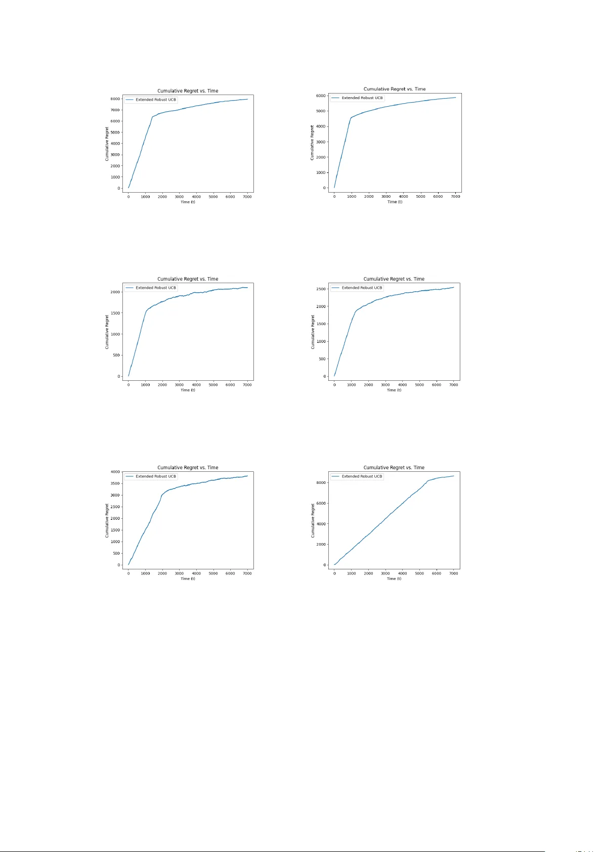
Extended UCB Policies for Multi-armed Bandit Problems

Extended UCB P olicies for Multi-Armed Bandit Problems Keqin Liu 1* , Tiansh uo Zheng 2 and Zhi-Hua Zhou 3,4 1* Sc ho ol of Mathematics and Ph ysics, Xi’an Jiaotong-Liverpo ol Univ ersity , 111 Ren’ai Road, Suzhou, 215123, Jiangsu, China. 2 Sc ho ol of Mathematics, Nanjing Univ ersity , 22 Hank ou Road, Nanjing, 210093, Jiangsu, China. 3 National Key Lab oratory for No v el Soft w are T echnology , 163 Xianlin Road Road, Nanjing, 210023, Jiangsu, China. 4 Sc ho ol of Artificial Intelligence, Nanjing Univ ersity , 163 Xianlin Road, Nanjing, 210023, Jiangsu, China. *Corresp onding author(s). E-mail(s): keqin.liu@xjtlu.edu.cn ; Con tributing authors: 221501001@smail.nju.edu.cn ; zhouzh@nju.edu.cn ; Abstract The m ulti-armed bandit (MAB) problems are widely studied in fields of op era- tions researc h, sto c hastic optimization, and reinforcemen t learning. In this paper, w e consider the classical MAB mo del with hea vy-tailed rew ard distributions and in tro duce the extended robust UCB p olicy , which is an extension of the results of Bubeck et al. [ 5 ] and Lattimore [ 22 ] that are further based on the pioneer- ing idea of UCB p olicies [e.g. Auer et al. 3 ]. The previous UCB p olicies require some strict conditions on rew ard distributions, whic h can b e difficult to guar- an tee in practical scenarios. Our extended robust UCB generalizes Lattimore’s seminary work (for moments of orders p = 4 and q = 2 ) to arbitrarily chosen p > q > 1 as long as the t wo momen ts ha ve a kno wn con trolled relationship, while still ac hieving the optimal regret growth order O (log T ) , th us providing a broadened application area of UCB policies for hea vy-tailed rew ard distributions. F urthermore, we achiev e a near-optimal regret order without any knowledge of the rew ard distributions as long as their p -th momen ts exist for some p > 1 . Finally , w e briefly present our earlier work on ligh t-tailed rew ard distributions for a complete illustration of the amazing simplicity and p o wer of UCB p olicies. 1 1 In tro duction As a protot yp e of reinforcemen t learning, a classical m ulti-armed bandit (MAB) model consists of a pla y er and a bandit machine with K arms. Under resource constrain ts, the play er can only choose one arm to pull at each time step. The ob jective of the pla yer is to identify and select the b est arm so that the long-term exp ected reward is maximized. Clearly , the pla yer’s action inv olves balancing the trade-off betw een exploration and exploitation, i.e., choosing an arm to learn its statistics vs. choosing an arm app earing to b e b est based on past observ ations. Sp ecifically , each arm i offers a random reward according to an unknown distribution X i when pulled by the play er (or agent). Each rew ard distribution has a mean, sa y θ i . The play er who has limited kno wledge ab out the underlying reward distributions (no knowledge ab out the means { θ i } ), has to c ho ose only one of these arms to play and accrue a rew ard at eac h time step, given the reward history so far observed. The play er aims to maximize the rew ard rate that accrues as the time horizon T grows. In many applications of online decision-making problems, such as Internet advertising and recommendation systems, the MAB mo del is widely assumed, with n umerous algorithms proposed for efficient reinforcemen t learning, e.g. Zhao [ 38 ], Lattimore and Szep esv´ ari [ 23 ]. W e p oin t out that the w ay kno wledge is acquired becomes crucial to maximizing the long-term rew ard rate in mo dern AI systems [ 31 ]. Since knowledge can b e treated as data in general, the struggle b etw een exploration (sampling) and exploitation (consuming) as a fundamental dilemma is expressly reflected in the MAB mo del [ 3 , 5 , 21 , 24 , 28 ]. T o address the k ey issue in the conflict b et ween exploration and exploitation, w e emphasize on the fact that it is imp ossible for the play er to know exactly the sp ecific v alues of rew ard means within any finite horizon of time. Instead, the only information the play er p ossesses is the (lo cal) reward history , and the play er has to learn from this to make a decision at each time step. Based on the limited historical information, the pla yer has to choose b etw een tw o sp ecific options. The first option is to explore an apparen tly suboptimal arm with a lo wer a verage rew ard, as there is alwa ys a p ossibility that the truly b est arm may not giv e the b est av erage rew ard in the past sample path. The second option is to exploit an arm with the highest av erage reward offered so far. Robbins [ 28 ] considered a simple t w o-armed bandit mo del and sho wed that there is a p olicy to achiev e the b est av erage reward asymptotically as time go es to infinity . Man y y ears later,Lai and Robbins [ 21 ] proposed a muc h stronger p erformance measure referred to as regret, whic h represen ts the exp ected total loss compared to the ideal scenario in which the play er kno ws which arm has the highest reward mean from the v ery beginning. Giv en a set of K arms with reward distributions F = { F 1 , F 2 , . . . , F K } with means { θ i } K i =1 and a p olicy π , the regret R F π ( T ) is defined as (without loss of generalit y , w e can assume that θ 1 ≥ θ i for 1 ≤ i ≤ K ) R F π ( T ) = X θ i <θ 1 E [ s i ( T )]∆ i , (1) where ∆ i = θ 1 − θ i , (2) 2 and s i ( T ) denotes the n umber of times that arm i w as chosen during time steps 1 to T under the p olicy π . Certainly , a low er regret growth rate indicates b etter p erformance of a p olicy and also a higher efficiency of learning. F urthermore, any sublinear regret order with T implies the asymptotic ac hiev ement of the maximum time-a verage rew ard as T → ∞ . Strikingly , Lai and Robbins [ 21 ] pro v ed an asymptotic lo wer b ound O (log T ) on the regret gro wth rate, under the assumption that the probability density/mass function of eac h reward distribution has the form f ( · ; θ ), where f is kno wn but parameter θ is unknown. They also prop osed an asymptotically optimal policy for a family of distributions, under which the optimal regret can b e achiev ed asymptotically , b oth the logarithmic order and the leading co efficien t. Auer et al. [ 3 ] proposed a class of p olicies featured b y UCB (upp er confidence bound), ac hieving logarithmic regret if the rew ard distributions hav e finite supp ort on a closed interv al [ a, b ] ⊂ R with a, b ∈ R kno wn to the play er. Their UCB1 and UCB1-T uned p olices perform very w ell for the classical MAB problem with a theoretically pro ven regret bound for any finite time horizon. UCB p olicies are widely applied in machine learning dev elopments (e.g. recommendation systems [ 17 , 32 ]) and in v arious reinforcement learning algorithms suc h as Mon te Carlo T ree Search (MCTS) [ 20 ], which is frequently used in gaming AIs [ 27 ] and forms a k ey step in the design of AlphaGo Zero [ 16 ]. 1.1 Ligh t-T ailed and Heavy-T ailed MAB Mo dels In the literature, MAB was first addressed under the assumption that all reward dis- tributions are light-tailed, i.e., the sample mean conv erges to the true mean faster so learning b ecomes easier compared to the hea vy-tailed case. Specifically , light-tailed (or sub-Gaussian) distributions usually hav e only a relatively small probability of pro- ducing a significan tly shifted random sample from its exp ectation; while heavy-tailed distributions hav e a relatively high probabilit y of pro ducing a large deviation. There are several p opular light-tailed probability distributions, suc h as Bernoulli, Gaussian, Laplacian, and Exp onen tial. Sp ecifically , the class of light-tailed distributions requires the (local) existence of the moment-generating function of the asso ciated random v ariable and is therefore referred to as the lo cally sub-Gaussian distributions [ 10 ]. F or- mally , a random v ariable X is called light-tailed if there exists some u 0 > 0 such that its moment-generating function is well defined on [ − u 0 , u 0 ] [ 10 ]: M ( u ) := E [exp( uX )] < ∞ , ∀| u | ≤ u 0 . (3) The ab o ve condition is equiv alen t to [ 10 ]: E [exp( u ( X − E X ))] ≤ exp( ζ u 2 / 2) , ∀| u | ≤ u 0 , ∀ ζ ≥ sup | u |≤ u 0 M (2) ( u ) , (4) where M (2) ( · ) denotes the second deriv ative of M ( · ). Note that the ab ov e upp er bound on M ( u ) has a form of the moment-generating function of the Gaussian distribution, th us the name “sub-Gaussian” has b een adopted. 3 The terminology “heavy-tailed”, opposite to “ligh t-tailed”, implies that the rew ard distribution can pro duce large v alues with high probabilities, leading to nonexistence of its momen t-generating function (even lo cally). Compared to the ligh t-tailed class, the heavy-tailed one is harder to learn in terms of the rank of their means. Bub ec k et al. [ 5 ] prop osed the robust UCB algorithm, under the assumption that there exists a kno wn p > 1 suc h that E [ | X i | p ] exists and is upper bounded by a kno wn parameter, for all 1 ≤ i ≤ K . Robust UCB shows significant progress for the heavy-tailed MAB mo del by ac hieving the optimal logarithmic order of regret growth. Subsequently , Lattimore [ 22 ] developed a new UCB p olicy referred to as the sc ale fr e e algorithm . This algorithm remov es the general assumption of a known upp er b ound on the p - th moment. Instead, it allo ws the v ariance and the squared fourth moment to scale freely as long as their ratio (kurtosis) is b ounded by a known parameter. But this assumption restricts p to b e no less than 4 (not too hea vy-tailed). In this paper, w e extend Lattimore’s work to any p > 1 with a tighter regret upp er b ound in the case of p = 4 with low discrimination where arm means are close and learning the arm rank b ecomes c hallenging. First, we assume that the pla y er knows a constant C p,q for some p and q ( p > q > 1) suc h that 1 E [ | X − E X | p ] ≤ C p,q [ E [ | X − E X | q ] ] p/q . (5) W e p oin t out that the kno wledge of sp ecific v alues of p and q is not required. F urther- more, the requirement of knowledge of C p,q can also b e remo v ed with an arbitrarily small sacrifice of the regret order as seen in Sec. 2.1 . The ab o ve inequality is a direct generalization of the assumption of kurtosis in Lattimore [ 22 ] where p = 4 and q = 2. F or a sp ecific example, supp ose that X has a P areto distribution of type II I with cum ulative distribution function [ 2 ] F ( x ) =    1 −  1 +  x − a σ  1 /γ  − 1 , x > a 0 , x ≤ a , where 0 < γ < 1 and σ > 0. Simple computations sho w that E [ | X − E X | p ] = C ( p, q , γ ) [ E [ | X − E X | q ] ] p/q for 1 < q < p < 1 /γ , where I ( p, γ ) := Z + ∞ 0  x − γ π sin γ π  p x 1 /γ γ x (1 + x 1 /γ ) 2 d x, C ( p, q , γ ) = I ( p, γ ) /I ( q , γ ) p/q . Note that the moment of this distribution is a function of σ . When σ increases, the momen t of any fixed order also increases if it exists. The robust UCB p olicy requires 1 By Jensen’s inequality , the existence of the p -th moment implies the existence of the q -th moment for any 1 < q < p . 4 the knowledge of p and an upp er b ound of the p -th momen t [ 5 ]. Therefore, for an arm with an unknown σ , w e cannot apply the robust UCB p olicy . F urthermore, le arning efficiency can b e improv ed if a larger p can b e used (tighter b ound on the tail, but the corresp onding momen t bound b ecomes harder to kno w or compute a priori ). It is thus b etter to eliminate the need for any prior kno wledge regarding the sp ecific v alues or b ounds on the moments. This motiv ates Lattimore [ 22 ] to consider the scale free algo- rithm. How ev er, Lattimore’s algorithm requires sp ecific v alues of p and q ( p = 2 q = 4) and cannot deal with the v ery heavy-tailed case (for p close to 1). Such requirements significan tly limited the application of the scale free algorithm. In contrast, our algo- rithm only requires p > 1 while p can b e unkno wn or unspecified. F urthermore, our algorithm achiev es near-optimal regret even without any sp ecific kno wledge on the rew ard distributions including C p,q . These results significantly broaden the applica- bilit y of the scale free algorithm. After we generalize Lattimore’s work, we will give a correction to a minor flaw of a lemma in Bub ec k et al. [ 5 ] that subsequently caused a small error in the computation of the regret upp er b ound in Lattimore [ 22 ]. 1.2 Related W ork The theory of frequen tist MAB has b een developed for a long perio d of time, and v arious milestones hav e b een made since Lai and Robbins [ 21 ]. In con trast to the Ba yesian mo del, the frequentist MAB do es not assume a priori kno wledge of the initial probabilit y or state of the system but learns the core parameters solely through the past sampling history , e.g., computing an upp er confidence b ound as a function of the frequency that an arm is selected and the v alues of the observed samples. This wa y of decision-making in the balance of exploration with exploitation contrasts with the Ba yesian mo del in whic h the tradeoff is usually addressed b y dynamic programming for the transitional characteristics of the system or the observ ation mo del [ 13 ]. After the UCB1 policy b y Auer et al. [ 3 ], many other policies of the UCB class hav e been prop osed in the literature. Maillard et al. [ 26 ] directed their attention to the prosp ect of KL div ergence betw een probabilit y distributions. They in tro duced the KL-UCB algorithm, which notably tightened the regret b ound. This improv emen t was ac hieved under the assumption of bounded rewards with known bounds. F urthermore, KL- UCB p olicy achiev es the asymptotic low er b ound of regret growth rate for this class of rew ards given in Burnetas and Katehakis [ 6 ]. Kaufmann et al. [ 19 ] com bined the Ba yesian metho d with the UCB class and prop osed Bay es-UCB for b ounded rewards with known b ounds, achieving a theoretical regret b ound similar to that of KL-UCB. Numerical exp erimen ts demonstrated the high efficiency of learning b y Bay es-UCB for Gaussian rew ard distributions. A surv ey of such UCB policies can b e found in Burtini et al. [ 7 ]. These p olicies w ere neither implemen ted nor prov ed to achiev e the logarithmic regret growth in the case of unbounded rew ard distributions. In 2011, the first author of this pap er prop osed UCB1-L T with a pro ven logarithmic upp er b ound on the regret growth rate for the class of all light-tailed rew ard distributions [ 24 ], filling the gap for the case of unbounded ligh t-tailed reward distributions. T ogether with the extended robust UCB for the heavy-tailed class focused in this pap er, w e provide a relativ ely complete picture of UCB p olicies for general reward distributions. W e will first present our UCB p olicy for the hea vy-tailed class as the main con tent of this 5 pap er, follo wed b y a brief presentation of UCB1-L T. These results demonstrate the simplicit y and strong p erformance of UCB for all rew ard distributions. The UCB for the hea vy-tailed case is of course more complicated b ecause the pla yer needs to extract more information from past observ ation in con trast to the simple form (e.g. sample mean) of UCB as in the ligh t-tailed case. After 2011, Bub eck and Cesa-Bianchi [ 4 ] extended UCB1-L T to ( α , ψ )-UCB under a more general assumption that the (ligh t- tailed) reward moment-generating function is b ounded by a conv ex function ψ for all u ∈ R . F or the case of heavy-tailed reward distributions, we hav e men tioned that Bub ec k et al. [ 5 ] prop osed the robust UCB policy under the assumption that an upp er bound of the moments is known. The robust UCB p olicy uses different mean estimators rather than the empirical one and remark ably ac hieves the logarithmic regret gro wth rate. Under certain regularity conditions, the robust UCB p olicy may adopt three different mean estimators: the truncated mean estimator, the median-of-means estimator, and the Catoni mean estimator [ 8 ]. The truncated mean estimator requires the knowledge of an upp er b ound on the origin moments, which is not very effective in the case that the rew ard mean is far a wa y from zero. The median-of-means estimator considers the (cen tral) moment and th us patc hes up the deficiency of the truncated mean estimator: the mean estimation will not b e affected when the rew ard distributions are transformed b y translations. The Catoni mean estimator is more complicated and can only be used when the rew ard distributions hav e v ariances ( p ≥ 2). But when applied in the robust UCB policy , it gives a m uc h smaller regret co efficien t than the other tw o estimators. Recently , Chen et al. [ 11 ] show ed the result of applying the Catoni mean estimator to the case of p < 2, but the p erformance was not prov en to be b etter than the truncated mean and the median-of-means estimators. Finer estimations when extending the Catoni mean estimator to the case of p < 2 are interesting for future in vestigations. Several recent pap ers also considered the heavy-tailed MAB model and made significan t progress. W ei and Sriv asta v a [ 36 ] proposed the robust MOSS p olicy with logarithmic regret growth. Agra wal et al. [ 1 ] established a p olicy called KL inf -UCB, whic h achiev es a logarithmic upp er b ound on regret v ery close to the asymptotic lo wer b ound pro ved by Burnetas and Katehakis [ 6 ]. F or other non-classical MAB models, the hea vy-tailed model has also b een considered [ 30 , 37 ]. Ho wev er, these p olicies do not eliminate the knowledge requirement of an upp er b ound of moments, whic h has b een remo v ed from the extended robust UCB p olicy proposed in this paper. Note that Genalti et al. [ 12 ] considered the case where no kno wledge of the momen ts is a v ailable except for the existence of momen ts of order greater than 1, but a relatively strong assumption of the distribution (a larger probability mass on the negative semi- axis) was needed to achiev e logarithmic regret. There are also p olicies without follo wing the idea of UCB. The ϵ -greedy p olicy w as well studied, and many p olicies were prop osed using its idea, e.g., the constan t ϵ - decreasing p olicy [ 34 ], GreedyMix [ 9 ], and ϵ n -greedy [ 3 ]. The Deterministic Sequencing of Exploration and Exploitation (DSEE) policy [ 25 , 33 ] also ac hiev es logarithmic regret for both cases of single play er and multiple play ers (with kno wledge of upp er bound on momen ts). Other recent progresses on v arian ts of MAB, such as adv ersarial bandits, con textual bandits, and linear bandits, can b e found in [ 14 , 18 , 23 ]. In the follo wing 6 table, w e list the main results found in the literature for classical MAB with hea vy- tailed reward distributions for comparisons with ours. Papers Results Logarithmic Regret Bound Assumption Bubeck et al. [ 5 ] P i :∆ i > 0  v ∆ i  1 /ϵ log T E [ | X i − θ i | 1+ ϵ ] ≤ v (known) , ∀ i Lattimore [ 22 ] P i :∆ i > 0  ( κ − 1)∆ i + σ 2 i ∆ i  log T Kurt[ X i ] ≤ κ (known) , ∀ i, σ i := p V ar( X i ) W ei and Sriv astav a [ 36 ] P i :∆ i > 0 log T ∆ 1+ ϵ ϵ i K ! 1 ∆ 1 /ϵ i E [ | X i − θ i | 1+ ϵ ] ≤ v (known) , ∀ i Agraw al et al. [ 1 ] † P i :∆ i > 0 log T K L inf ( F i ,θ 1 ) E [ | X i − θ i | 1+ ϵ ] ≤ v (known) , ∀ i Genalti et al. [ 12 ] P i :∆ i > 0   v ∆ i  1 /ϵ + ∆ i P ( X i  =0)  log T E [ X 1 1 {| X 1 | >M } ] ≤ 0 , ∀ M ≥ 0 Ours P i :∆ i > 0 ∆ i  144(1 + C p,q )(6 v 1 q q + 2 q )(∆ i + 1 ∆ i )  M ( p,q ) log T , wher e M ( p, q ) = 1 / [(1 − 1 q )(1 − q p )] > 1 v p /v p/q q ≤ C p,q (known) , 1 < q < p, ∀ i, v l := E [ | X i − θ i | l ] † K L inf ( η, x ) := inf { K L ( η , F ) : E [ | X | 1+ ϵ ] ≤ v and E X ∼F [ X ] ≥ x } 2 Hea vy-T ailed Rew ard Distributions 2.1 The Extended Robust UCB P olicy Consider K arms offering random rewards { X 1 , X 2 , . . . , X K } with heavy-tailed distri- butions F = { F 1 , F 2 , . . . , F K } . In con trast with the light-tailed class, a heavy-tailed distribution may yield a very high (or low) reward realization with a high probability . Consequen tly , the empirical mean estimator X i,s = 1 s P s j =1 X i,j for a sequence of i.i.d. random v ariables { X i,j } s j =1 ma y not work prop erly to estimate the exp ectation of X i for arm i . The app endix of Bub eck et al. [ 5 ] has shown that under the assumption of hea vy-tailed distributions, with probability at least 1 − δ , 1 s s X j =1 X i,j ≤ θ i +  3 E | X i − θ i | r δ s r − 1  1 r , where 1 < r ≤ 2. Ho w ever, this bound is to o loose to obtain a UCB p olicy for ac hieving logarithmic regret gro wth. T o remedy this issue, w e adopt the median-of- means estimator prop osed in Bub eck et al. [ 5 ]. Definition 1 F or a finite i.i.d. sequence of random v ariables { X i,j } s j =1 dra wn from a distri- bution F i , define the median-of-means estimator ˆ µ ( { X i,j } s j =1 , k ) with k ( k ≤ s ) bins as the median of k empirical means    1 N ( l +1) N X j = lN +1 X i,j    k − 1 l =0 , where N = ⌊ s/k ⌋ . The following lemma offers an appro ximation of the pro ximity betw een the median- of-means estimator, utilizing a sp ecific num b er of bins, and the actual mean. It should b e noted that this lemma is similar to Lemma 2 in Bub eck et al. [ 5 ]. How ever, there is a minor flaw in the pro of of the latter, which will b e explained later. Moreov er, there exist differences b et w een the tw o lemmas, prompting us to restate and establish their distinctions in the following exp osition. 7 Lemma 1 Given any ϵ > 0 . Supp ose that log δ − 1 > 1 /ϵ, s ≥ (8 + ϵ ) log δ − 1 8 log( δ − 1 ) + 1 ϵ log( δ − 1 ) − 1 and v = E [ | X i − θ i | p ] < ∞ for some p such that p > 1 . Then with pr ob ability at le ast 1 − δ , the me dian-of-me ans estimator ˆ µ ( { X i,j } s j =1 , ⌈ 8 log δ − 1 ⌉ ) ≥ θ i − (12 v ) 1 /p  (8 + ϵ ) log ( δ − 1 ) s  ( p − 1) /p . Also, with pr ob ability at le ast 1 − δ , ˆ µ ( { X i,j } s j =1 , ⌈ 8 log δ − 1 ⌉ ) ≤ θ i + (12 v ) 1 /p  (8 + ϵ ) log ( δ − 1 ) s  ( p − 1) /p . With the help of the median-of-means estimator, w e can now define the upper confidence b ound for the extended robust UCB p olicy . As mentioned in ( 5 ), w e first assume that for an y arm distribution X i ∈ F with mean θ i , there is a known moment con trol co efficien t C p,q (1 < q < p ) such that E [ | X i − θ i | p ] ≤ C p,q [ E [ | X i − θ i | q ]] r , (6) where r = p/q . Definition 2 Let k = ⌈ 8 log δ − 1 ⌉ , χ = (8+ ϵ ) log δ − 1 s . Giv en an arbitrary ϵ > 0, a moment order p > 1, another moment order 1 < q < p , and the moment con trol co efficien t C p,q , define the upp er confidence bound of the extended robust UCB as (v alue of the fraction is set to + ∞ if divided by 0) ˜ µ ( { X i,j } s j =1 , δ ) := sup          θ ∈ R : θ ≤ ˆ µ ( { X i,j } s j =1 , k ) + 12 ˆ µ ( {| X i,j − θ | q } s j =1 , k ) max  0 , 1 − C ′ χ ( p − q ) /p  ! 1 /q χ ( q − 1) /q          , where C ′ = (12( C p,q + 1)) q /p . (7) Note that this upper confidence bound alwa ys exists, since the left-hand side of the ab o v e inequality tends to −∞ as θ → −∞ , while the right-hand side tends to + ∞ . Lemma 2 Supp ose that the c onditions in Lemma 1 ar e satisfie d, then with pr ob ability at le ast 1 − 2 δ , we have ˜ µ ( { X i,j } s j =1 , δ ) ≥ θ i . Corollary 1 Under the c onditions of L emma 1 , with pr ob ability at le ast 1 − δ , we have ˆ µ ( { Y i,j } s j =1 , k ) − v q ≤ C ′ v q χ ( p − q ) /p . 8 Please see ( 27 ) for the definitions of Y i,j , v q , Y i , v p . Finally , with the upper confidence b ound ˜ µ ( { X i,j } s j =1 ), we complete the extended robust UCB p olicy as follo ws. Algorithm 1: The Extended Robust UCB Policy π ∗ Input: ϵ > 0, K : the num b er of arms Initialize: s i ← 0 and { X i,j } s i j =1 an empty sequence for each arm i , 1 ≤ i ≤ K for t ← 1 to T do for i ← 1 to K do if s i = 0 then Set arm i ’s upp er confidence b ound to + ∞ end else Compute arm i ’s upp er confidence b ound as ˜ µ ( { X i,j } s i j =1 , t − 2 ) end end Cho ose an arm j that maximizes the upp er confidence b ound and obtain rew ard x Up date: s j ← s j + 1 and app end x to sequence { X j,k } s j k =1 end Here we present the main theorem that the extended robust UCB p olicy achiev es the logarithmic order of regret gro wth. Theorem 1 Supp ose p > q > 1 such that the p -th or der moments exist for al l F i ∈ F and ( 6 ) is satisfie d with known C p,q . Then for any ϵ > 0 , the r e gr et R F π ∗ ( T ) of the extende d r obust UCB p olicy π ∗ has the lo garithmic or der with r esp e ct to the time horizon T . Sp e cific al ly, we have R F π ∗ ( T ) ≤ P i :∆ i > 0 C i ( T )∆ i with C i ( T ) := h 36(1 + 8 ϵ ) + (16 + 2 ϵ )  144(1 + C p,q )(6 v 1 q q + 2 q )(∆ i + 1 ∆ i )  M ( p,q ) i log T + 11 , wher e M ( p, q ) := 1 / ((1 − 1 q )(1 − q p )) and T ≥ 9 2 ϵ + 3 2 . F rom the ab o v e, we observ e that the upp er b ound on regret increases with C p,q but decreases with p . This matc hes the in tuition that a tigh ter known b ound on the momen t ratio or a higher moment order adopted mak es the learning process easier due to less v ariation assumed in the samples. F urthermore, for an y fixed q , the upper b ound increases with v q . This is also easy to explain since a larger moment indicates a larger deviation from a sample to the true mean. Mean while, if q increases and b ecomes close to p , then the denominator of M ( p, q ) will approach 0 and the upp er b ound b ecomes w orse. This is because a larger v alue of p/q offers more global information on moments with different orders to facilitate the learning of the unknown distributions. Also, as ∆ i → 0 for some i , the upper b ound goes to infinity (since M ( p, q ) > 1) because it will b e harder to distinguish the b est arm from arm i . Finally , if the arm num b er K is increased with other parameters including ∆ i relativ ely fixed within the original 9 orders, the upp er b ound is clearly increased linearly with K due to the definition of regret. T o pro ve Theorem 1 , we just need to show the following core lemma to b ound the time s i sp en t on each sub optimal arm i b y the extended robust UCB p olicy . Lemma 3 The exp e cte d numb er of times E [ s i ( T )] that a sub optimal arm is chosen by the extende d r obust UCB p olicy π ∗ has an upper b ound of the lo garithmic or der with T . Sp e cific al ly, we have E [ s i ( T )] ≤ C i ( T ) wher e C i ( T ) is define d ab ove. Finally , we conduct Mon te Carlo sim ulation examples based on Laplace distribu- tions, Student-t distributions, and P areto distributions of type I I I (see Sec. 1.1 ). F rom Fig. 1 – 4 , w e observ e that the regret rate gro ws linearly at the b eginning to prepare the ground for ranking until at least one arm has a finite UCB (i.e., χ defined in ( 24 ) b ecomes sufficien tly small such that, within the sup op erator of ˜ µ ( { X i,j } s i j =1 , t − 2 ), not only the denominator is nonzero but also the gro wth rate of the righ t-hand side with θ becomes small). In Fig. 1 , w e compare the actual regret for different v alues of C p,q and observ e that the regret becomes larger for larger C p,q . In Fig 2 , the regret becomes smaller as p become s larger. F urthermore, the regret increases with v q and K as sho wn in Fig. 3 and Fig. 4 , resp ectively . All these observ ations match our theoretical analysis on the upp er b ound ab o ve. (a) Laplace with C p,q = 1 . 68 × 10 3 (b) Student-t with C p,q = 2 . 09 × 10 3 Fig. 1 : Comparison for different C p,q Note that if C p,q is unknown, then the play er can simply choose any increasing function f with f ( t ) → + ∞ as t → + ∞ to replace C p,q and ac hiev e a regret arbitrarily close to logarithmic order without requiring any knowledge of the reward moments (see App endix F for a pro of ). 10 (a) Pareto I II with p = 12 (b) Pareto I II with p = 15 Fig. 2 : Comparison for different p (a) Laplace with v q = 24 (b) Laplace with v q = 384 Fig. 3 : Comparison for different v q (a) Student-t with K = 2 (b) Student-t with K = 4 Fig. 4 : Comparison for different K 11 2.2 F urther Analysis and Comparison of The Extended Robust UCB No w we consider the sp ecific chosen v alues of p and q to further improv e the efficiency of the extended robust UCB p olicy . Case 1. Supp ose that the p ′ -th order of m omen ts of rew ard distributions exists with p ′ > 2 for all arms. Then we can choose p and q such that p = 2 q ≤ p ′ . Inequality ( 29 ) can b e refined to E [ | Y i − v q | p/q ] = E Y 2 i + v 2 q − 2 v q E Y i = E Y 2 i − v 2 q = v p − v 2 q ≤ ( C p,q − 1) v p/q q . (8) Hence, we can refine C ′ from ( 7 ) to C ′ = q 12( C p,q − 1) , (9) whic h can b e muc h smaller than the original definition ( 7 ). Next, we lo ok at the definition of χ M in App endix E that guaran tees the three inequalities ( 39 ), ( 40 ) and ( 41 ) to hold. The refinement of C ′ leads to a smaller right- hand side for all these inequalities, i.e. the constant χ M will b e larger and the regret upp er b ound will be smaller, which further implies that the p olicy’s selection will con verge to the b est arm faster. Case 2. Assume that the 4-th order of momen ts of reward distributions exists as in Lattimore [ 22 ]. Then we can c ho ose p = 4 and q = 2. In this case, our UCB in Definition 2 can b e rewritten as ˜ µ ( { X i,j } s j =1 , δ ) := sup        θ ∈ R : θ ≤ ˆ µ ( { X i,j } s j =1 , k ) + s 12 ˆ µ ( { ( X i,j − θ ) 2 } s j =1 , k ) max  0 + , 1 − C ′ √ χ  χ        . In other words, C p,q degenerates to an upper b ound on kurtosis. The function B ( x ) defined in ( 36 ) b ecomes B ( x ) = 24 τ ( x ) 1 − 48 xτ ( x )  1 + C ′ √ x  + 576 √ xτ ( x ) 1 − 48 xτ ( x ) , and the three inequalities ( 39 ), ( 40 ) and ( 41 ) are refined to 1 > C ′ √ x, (10) 1 > 48 xτ ( x ) , (11) ∆ i ≥ √ v 2 x  p B ( x ) + 2 √ 3  . (12) Under these refined estimations for χ M , the leading co efficient of log T in ( 46 ) is significan tly reduced. Now we compare the extended robust UCB and the scale free 12 algorithm proposed in Lattimore [ 22 ], under the same assumption sp ecified at the b eginning of Case 2. W e first address a flaw of Lemma 2 in Bubeck et al. [ 5 ]. This lemma, crucial in Lattimore [ 22 ] for deriving the regret upper b ound of the scale free algorithm, is examined more closely below. F or clarit y and coherence with the notation employ ed in this pap er, we present the follo wing adapted version. A Flawe d Statement in Bub e ck et al. [ 5 ] : Let δ ∈ (0 , 1) and p ∈ (1 , 2]. Let { X i,j } s j =1 b e i.i.d. random v ariables with mean E X i = θ i and (cen tered) p -th momen t v p . Let k ′ = ⌊ min { 8 log (e 1 / 8 δ − 1 ) , s/ 2 }⌋ . Then with probability at least 1 − δ , ˆ µ  { X i,j } s j =1 , k ′  ≤ θ i + (12 v p ) 1 /p  16 log (e 1 / 8 δ − 1 ) s  ( p − 1) /p . The last inequality in the pro of of this statement in Bub ec k et al. [ 5 ] assumes that exp( − k ′ / 8) ≤ δ , equiv alen t to k ′ ≥ 8 log δ − 1 . How ever, the definition of k ′ in this statemen t is k ′ = ⌊ min { 8 log (e 1 / 8 δ − 1 ) , s/ 2 }⌋ . In the following, we give the corrected version of the ab o v e statement. Lemma 4 L et δ ∈ (0 , 1) and p ∈ (1 , 2] . L et { X i,j } s j =1 b e i.i.d. r andom variables with me an E X i = θ i and (c enter e d) p -th moment v p , wher e s is chosen such that ⌊ s/ 2 ⌋ ≥ 8 log δ − 1 . L et k ′ = ⌊ min { 8 log(e 1 / 8 δ − 1 ) , s/ 2 }⌋ . Then with pr ob ability at le ast 1 − δ , ˆ µ  { X i,j } s j =1 , k ′  ≤ θ i + (12 v p ) 1 /p 16 log(e 1 / 8 δ − 1 ) s ! ( p − 1) /p . The next theorem shows that with a prop erly chosen parameter ϵ > 0, the upp er b ound given in ( 46 ) is also tighter than that in Lattimore [ 22 ] in long run if ∆ i is small, i.e., arms are hard to b e distinguished (the low-discrimination case). In the following theorem, we formally state this result while correcting the upp er b ound in Lattimore [ 22 ] by Lemma 4 . Theorem 2 Choose any 8 < ϵ < 280 − 16 √ 2 2 √ 2+3 ( ≈ 44 . 158 ) and let δ = t − 2 . The upp er b ound given in L attimor e [ 22 ] of E [ s i ( T )] is gr e ater than that given in ( 46 ) for sufficiently lar ge T and sufficiently smal l ∆ i . That is, after dividing b oth r e gr et upp er b ounds by log δ − 1 and letting T → + ∞ , we have (8 + ϵ )  8 ϵ + max  8 ϵ , 1 χ M  < 3648 max  ( C ′ ) 2 12 , v 2 ∆ 2 i  + 16 (13) for sufficiently smal l ∆ i . The r e gr et upp er b ound of the sc ale fre e algorithm pr op ose d in L attimor e [ 22 ] is thus asymptotic al ly lar ger than that of the extende d robust UCB p olicy for ϵ ∈ (8 , 280 − 16 √ 2 2 √ 2+3 ) . 13 F urthermore, we show that the regret of the extended robust UCB deviates from the theoretical low er b ound (in the non-parametric setting) by only a constant factor and a constant term as in the scale free algorithm of Lattimore [ 22 ]. First, we restate the low er b ound derived in Lattimore [ 22 ] as follows. Theorem 3 L et H κ 0 b e the set of distributions that have kurtosis less than κ 0 . Assume ∆ > 0 and κ 0 ≥ 7 / 2 . Supp ose that X ∈ H κ 0 has a me an of µ , a positive varianc e of σ 2 , and a kurtosis of k . Then inf { KL( X, X ′ ) : X ′ ∈ H κ 0 and E [ X ′ ] > µ + ∆ } ≤ ( min {− log(1 − p ) , C 1 ∆ 2 σ 2 } , if C 0 √ k ( k + 1) ∆ σ < κ 0 − log(1 − p ) , otherwise , (14) wher e C 0 , C 1 > 0 ar e universal c onstants and p = min { ∆ /σ, 1 /κ 0 } . Based on this, we can dra w the following conclusion: Theorem 4 L et δ = t − 2 . Under Case 2, the r e gr et of the extende d r obust UCB p olicy applie d to H κ 0 ( κ 0 ≥ 7 / 2 ) differs fr om the lower b ound of r e gr et by a c onstant factor and a c onstant term. F urthermore, we give another upp er b ound that shows a sublinear regret in terms of arm num ber K . Recall the upper b ound on regret in Theorem 1 . W e ha ve R F π ∗ ( T ) = X i :∆ i > 0 ∆ i E [ s i ( T )] = X i :∆ i > 0 ∆ i [ E [ s i ( T )]] 1 / M ( p,q ) [ E [ s i ( T )]] 1 − 1 / M ( p,q ) ≤ X i :∆ i > 0 ∆ i h M 1 + M 2 ( p, q )( ∆ 2 i + 1 ∆ i ) M ( p,q )  2 log T i 1 / M ( p,q ) [ E [ s i ( T )]] 1 − 1 / M ( p,q ) ≤ X i :∆ i > 0 M 3 ( p, q )(∆ 2 i + 1)(log T ) 1 / M ( p,q ) [ E [ s i ( T )]] 1 − 1 / M ( p,q ) ≤ M 3 ( p, q )(log T ) 1 / M ( p,q ) h X i :1 ≥ ∆ i > 0 2[ E [ s i ( T )]] 1 − 1 / M ( p,q ) + X i :∆ i > 1 2∆ 2 i [ E [ s i ( T )]] 1 − 1 / M ( p,q ) i ≤ 2 M 3 ( p, q )(log T ) 1 / M ( p,q ) h K 1 / M ( p,q ) T 1 − 1 / M ( p,q ) + X i :∆ i > 1 ∆ 2 i T 1 − 1 / M ( p,q ) i ≤ M 3 ( p, q )(log T ) 1 / M ( p,q ) T 1 − 1 / M ( p,q ) h K 1 / M ( p,q ) + X i :∆ i > 1 ∆ 2 i i where M 1 = 19 + 144 /ϵ, M ( p, q ) = 1 / ((1 − 1 /q )(1 − q /p )) > 1 , T ≥ 9 2 ϵ + 3 2 , and M 2 ( p, q ) = (8 + ϵ )  144(1 + C p,q )(6 v 1 q q + 2 q )  M ( p,q ) , 14 M 3 ( p, q ) =  M 1 + 2 M 2 ( p, q )  1 / M ( p,q ) . It is desirable to remo ve the dependency of regret b ound on ∆ i as well and this will b e considered in the future work. 3 Ligh t-T ailed Rew ard Distributions W e p oin t out that our p olicy and results also w ork for the light-tailed reward distri- butions since our construction depends only on the existence of momen ts. Ho wev er, as mentioned in Sec. 1.2 , the UCB could b e significantly simplified for the light-tailed class where learning rew ard means b ecomes muc h easier. F urthermore, the leading constan t of the logarithmic regret upp er b ound can also b e greatly reduced as shown in [ 24 ]. Therefore, we now formally but briefly discuss the work in [ 24 ] that extended the UCB policy for distributions with known finite supp orts in [ 3 ] to all ligh t-tailed distributions. W e will also compare our work with some subsequent work following [ 24 ]. T ogether with ab o ve results for the heavy-tailed class, we see a complete picture of the b eaut y and p o wer of UCB as w ell as what information needs to b e extracted in its sp ecific design based on how the samples represent the true means. 3.1 The UCB1-L T Policy The empirical mean is adopted in estimating the upp er confidence b ound for the class of light-tailed rew ard distributions. As before, let X i,s denote the empirical mean 1 s P s j =1 X i,j for arm i , where { X i,j } s j =1 form the i.i.d. random reward sequence drawn from an unknown distribution X i ∈ F . Lemma 5 (Bernstein-typ e b ound) F or i.i.d. r andom variables { X i,j } s j =1 dr awn from a light- taile d distribution X i (with me an θ i ) with a finite moment-gener ating function M ( u ) over r ange u ∈ [ − u 0 , u 0 ] for some u 0 > 0 . We have, ∀ ϵ > 0 , P ( X i,s − θ i ≥ ϵ ) ≤ ( exp( − s 2 ζ ϵ 2 ) , ϵ < ζ u 0 exp( − su 0 2 ϵ ) , ϵ ≥ ζ u 0 , (15) wher e ζ > 0 satisfies ζ ≥ sup | u |≤ u 0 M (2) ( u ) . A similar b ound also holds for P ( X i,s − θ i ≤ − ϵ ) by symmetry. The pro of of the abov e lemma follo ws a similar argument as in V ershynin [ 35 ]. Using the Bernstein-type b ound by Lemma 5 , w e propose the UCB1-L T p olicy as follo ws. 15 Algorithm 2: The UCB1-L T Policy Input: a 1 ≥ 8 ζ , a 2 ≥ a 1 / ( ζ u 0 ), K : the num b er of arms Initialize: s i ← 0 and X i ← 0 for each arm i , 1 ≤ i ≤ K for t ← 1 to T do for i ← 1 to K do if s i = 0 then Assign + ∞ to the upp er confidence b ound end else if q a 1 log t s i < ζ u 0 then Compute the upp er confidence b ound as X i + q a 1 log t s i end else Compute the upp er confidence b ound as X i + a 2 log t s i end end end Cho ose an arm j that maximizes the upp er confidence b ound and obtain rew ard x X j ← x + s j X j s j +1 and s j ← s j + 1 end The UCB1-L T policy considers t wo upp er confidence bounds and alternatively uses one of them according to v alues of t and s i ( t − 1). T o minimize the theoretical regret upp er b ound, we can c ho ose a 1 = 8 ζ and a 2 = 8 u 0 . The following theorem shows that UCB1-L T achiev es logarithmic regret gro wth for the light-tailed reward distributions. Theorem 5 F or the light-taile d r ewar d distributions, the r e gr et of the UCB1-L T p olicy satisfies the fol lowing ine quality: R F π ( T ) ≤ X i : θ i <θ 1 ∆ i  max  4 a 1 ∆ 2 i , 2 a 2 ∆ i  log T + 1 + π 2 3  . (16) In App endix A , w e compare our UCB1-L T policy with the ( α, ψ )-UCB p olicy prop osed in Bub ec k and Cesa-Bianchi [ 4 ]. 4 Conclusion and Ac kno wledgmen t In this paper, we ha v e prop osed t w o order-optimal UCB p olicies, namely the extended robust UCB and UCB1-L T, dealing with the heavy-tailed and ligh t-tailed rew ard distributions in the frequentist m ulti-armed bandit problems, resp ectiv ely . W e are grateful for the help from Mr. Haoran Chen during the initial stage of this pro ject, and Dr. Y ao qing Y ang from Dartmouth College in improving this article. 16 References [1] Agra w al, S., Juneja, S. K. and Ko olen, W. M. (2021). Regret minimization in hea vy-tailed bandits. Pr o c e e dings of the Thirty F ourth Confer enc e on L e arning The ory, PMLR , 134:26–62. [2] Arnold, B. C. (2008). P areto and generalized pareto distributions. Mo deling Inc ome Distributions and L or enz Curves , 119–145. [3] Auer, P ., Cesa-Bianc hi, N. and Fisc her, P . (2002). Finite-time analysis of the m ultiarmed bandit problem. Machine L e arning , 47:235-256. [4] Bubeck, S. and Cesa-Bianchi, N. (2012). Regret analysis of sto c hastic and non- sto c hastic m ulti- armed bandit problems. F oundations and T r ends in Machine L e arning , 5:1-122. [5] Bubeck, S., Cesa-Bianc hi, N. and Lugosi, G. (2013). Bandits with heavy tail. IEEE T r ansactions on Information The ory , 59:7711-7717. [6] Burnetas, A. N. and Katehakis, M. N. (1996). Optimal adaptiv e p olicies for sequen tial allo cation problems. A dvanc es in Applie d Mathematics , 17:122-142. [7] Burtini, G., Lo eppky , J. and Lawrence, R. (2015). A surv ey of online exp erimen t design with the sto chastic multi-armed bandit. arXiv pr eprint [8] Catoni, O. (2012). Challenging the empirical mean and empirical v ariance: a deviation study . A nnales de l’I.H.P. Pr ob abilit´ es et statistiques , 48(4):1148–1185. [9] Cesa-Bianc hi, N. and Fischer, P . (1998). Finite-time regret b ounds for the m ul- tiarmed bandit problem. Pr o c e e dings of the Fifte enth International Confer enc e on Machine L e arning , 100-108. [10] Charek a, P ., Charek a, O. and Kennendy , S. (2006). Lo cally sub-gaussian ran- dom v ariable and the strong law of large n um b ers. Atlantic Ele ctr onic Journal of Mathematics , 1:75-81. [11] Chen, P ., Jin, X., Li, X. and Xu, L. (2021). Generalized catoni’s m-estimator under finite α -th moment assumption with α ∈ (1,2). Ele ctr onic Journal of Statistics , 15:5523-5544. [12] Genalti, G., Marsigli, L., Gatti, N. and Metelli, A. M. (2024). ( ϵ, u )-adaptiv e regret minimization in heavy-tailed bandits. Pr o c e e dings of Machine L e arning R ese ar ch , 247:1-34. [13] Gittins, J. C., Glazebro ok, K. D. and W eb er, R. R. (2011). Multi-Arme d Bandit A l lo c ation Indic es. Wiley , Chichester, 2nd Edition. 17 [14] Zhong, H., Huang, J., Y ang, L. and W ang, L. (2021). Breaking the moments condition barrier: No- regret algorithm for bandits with sup er heavy-tailed pay offs. A dvanc es in Neur al Information Pr o c essing Systems , 34:15710-15720. [15] Hoeffding, W. (1994). Probability inequalities for sums of b ounded random v ariables. The Col le cte d Works of Wassily Ho effding , 409–426. [16] Holcom b, S. D., Porter, W. K., Ault, S. V., Mao, G. and W ang, J. (2018). Ov erview on deepmind and its alphago zero ai. Pr o c e e dings of the 2018 International Confer enc e on Big Data and Educ ation , 67–71. [17] Ie, E., Hsu, C.-w., Mladeno v, M., Jain, V., Narv ek ar, S., W ang, J., W u, R. and Boutilier, C. (2019). Recsim: A configurable simulation platform for recommender systems. arXiv pr eprint [18] W ang, J., Zhao, P . and Zhou, Z. (2023). Revisitingw eighted strategy for non- stationary parametric bandits. Pr o c e e dings of the Twenty Sixth International Confer enc e on Artificial Intel ligenc e and Statistics, PMLR , 206:7913-7942. [19] Kaufmann, E., Capp´ e, O. and Garivier, A. (2012). On bay esian upp er confidence b ounds for bandit problems. Pr o c e e dings of the Fifte enth International Confer enc e on Artificial Intel ligenc e and Statistics, PMLR , 22:592-600 [20] Kocsis, L. and Szep esv´ ari, C. (2006). Bandit based mon te-carlo planning. Eur op e an Confer enc e on Machine L e arning , 282–293. [21] Lai, T. L. and Robbins, H. (1985). Asymptotically efficient adaptiv e allocation rules. A dvanc es in Applie d Mathematics , 6:4–22. [22] Lattimore, T. (2017). A scale free algorithm for sto chastic bandits with b ounded kurtosis. A dvanc es in Neur al Information Pr o c essing Systems , 30:1–10. [23] Lattimore, T. and Szepesv´ ari, C. (2020). Bandit A lgorithms. Cambridge Univ ersity Press. [24] Liu, K. and Zhao, Q. (2011a). Extended UCB p olicy for m ulti-armed bandit with ligh t-tailed reward distributions. arXiv pr eprint [25] Liu, K. and Zhao, Q. (2011b). Multi-armed bandit problems with hea vy-tailed rew ard distributions. 2011 49th Annual Al lerton Confer enc e on Communic ation, Contr ol, and Computing (A l lerton) , 485–492. [26] Maillard, O.-A., Munos, R. and Stoltz, G. (2011). A finite-time analysis of multi- armed bandits problems with kullback-leibler divergences. Pr o c e e dings of the 24th A nnual Confer enc e on L e arning The ory, PMLR , 19:497–514. [27] P o wley , E. J., Whitehouse, D. and Cowling, P . I. (2013). Bandits all the wa y down: UCB1 as a simulation p olicy in monte carlo tree search. 2013 IEEE Confer enc e on 18 Computational Intel ligenc e in Games (CIG) , 1–8. [28] Robbins, H. (1952). Some asp ects of the sequential design of exp erimen ts. Bul letin of the A meric an Mathematic al So ciety , 58:527–535. [29] Rudin, W. (1974). R e al and Complex A nalysis. T ata McGraw-Hill, 2nd Edition. [30] Shao, H., Y u, X., King, I. and Lyu, M. R. (2018). Almost optimal algorithms for linear stochastic bandits with hea vy-tailed pa yoffs. A dvanc es in Neur al Information Pr o c essing Systems , 31:8430-8439. [31] Silv er, D., Schritt wieser, J., Simony an, K., Antonoglou, I., Huang, A., Guez, A., Hub ert, T., Baker, L., Lai, M., Bolton, A. et al. (2017). Mastering the game of go without human knowledge. Natur e , 550:354-359. [32] Song, L., T ekin, C. and V an Der Schaar, M. (2014). Online learning in large- scale con textual recommender systems. IEEE T r ansactions on Servic es Computing , 9:433–445. [33] V akili, S., Liu, K. and Zhao, Q. (2013). Deterministic sequencing of exploration and exploitation for multi-armed bandit problems. IEEE Journal of Sele cte d T opics in Signal Pr o c essing , 7:759–767. [34] V ermorel, J. and Mohri, M. (2005). Multi-armed bandit algorithms and empirical ev aluation. In Eur op e an Confer enc e on Machine L e arning , 437–448. [35] V ershynin, R. (2010). Introduction to the non-asymptotic analysis of random matrices. arXiv pr eprint [36] W ei, L. and Sriv astav a, V. (2020). Minimax p olicy for hea vy-tailed bandits. IEEE Contr ol Systems L etters , 5:1423–1428. [37] Y u, X., Shao, H., Lyu, M. R. and King, I. (2018). Pure exploration of multi- armed bandits with hea vy-tailed pay offs. Pr o c e e dings of the 34th Confer enc e on Unc ertainty in Artificial Intel ligenc e , 937-946. [38] Zhao, Q. (2019). Multi-armed bandits: Theory and applications to online learning in netw orks. Synthesis L e ctur es on Communation Networks , 12:1-165. 19 A F rom UCB1-L T to ( α, ψ )-UCB After the establishment of UCB1-L T by Liu and Zhao [ 24 ], Bubeck and Cesa-Bianchi [ 4 ] subsequently prop osed the ( α, ψ )-UCB under a more general assumption on the momen t generating functions. Specifically , the ( α, ψ )-UCB p olicy assumes that the distribution of rew ard X i ∈ F satisfies the follo wing condition: there exists a conv ex function ψ defined on R such that for all λ > 0, log E h e λ ( X i − θ i ) i ≤ ψ ( λ ) and log E h e λ ( θ i − X i ) i ≤ ψ ( λ ) . (17) F or example, if X i is b ounded in [0 , 1] as assumed in UCB1, one can choose ψ ( λ ) = λ 2 8 and ( 17 ) becomes the w ell-known Ho effding’s lemma [ 4 ]. Since + ∞ is allow ed in the range of ψ , this assumption is more general than that in UCB1-L T. The Legendre- F renc hel transform ψ ∗ of ψ is defined as ψ ∗ ( ϵ ) := sup λ ∈ R λϵ − ψ ( λ ) . The upp er confidence b ound of ( α , ψ )-UCB at time t is defined as I i ( t ) := X i,s i ( t − 1) + ( ψ ∗ ) − 1  α log t s i ( t − 1)  . (18) Theorem 6 (Bub ec k and Cesa-Bianc hi [ 4 ]) Assume that the r eward distributions satisfy ( 17 ) . Then ( α, ψ ) -UCB with α > 2 achieves R F π ( T ) ≤ X θ i <θ 1  α ∆ i ψ ∗ (∆ i / 2) log T + α α − 2  . (19) F or the UCB1-L T p olicy , we can choose ψ ( λ ) = ( ζ λ 2 2 , λ ≤ u 0 + ∞ , λ > u 0 . (20) Then ( 17 ) b ecomes the same assumption as in UCB1-L T (see ( 4 )). In this case, we ha ve ψ ∗ ( ϵ ) = ( ϵ 2 2 ζ , | ϵ | < ζ u 0 u 0 ( | ϵ | − ζ u 0 2 ) , | ϵ | ≥ ζ u 0 . Th us the inv erse ( ψ ∗ ) − 1 ( x ) of ψ ∗ for x ≥ 0 will b e ( ψ ∗ ) − 1 ( x ) = ( √ 2 ζ x, 0 ≤ x < ζ u 2 0 2 x u 0 + ζ u 0 2 , x ≥ ζ u 2 0 2 . 20 F urthermore, if we choose α = 4, then the upper confidence b ound defined in ( 18 ) b ecomes I i ( t ) = X i,s i ( t − 1) +    q 8 ζ log t s i ( t − 1) , log t s i ( t − 1) < ζ u 2 0 8 4 log t u 0 s i ( t − 1) + ζ u 0 2 , log t s i ( t − 1) ≥ ζ u 2 0 8 . (21) If we choose a 1 = 8 ζ and a 2 = 8 u 0 in UCB1-L T, we get the same UCB under the condition log t s i ( t − 1) < ζ u 2 0 8 . F or the case log t s i ( t − 1) ≥ ζ u 2 0 8 , the upper confidence bound of ( α, ψ )-UCB is not larger than that of UCB1-L T and thus may ac hieve a smaller theoretical upp er b ound of regret as follows: R F π ( T ) ≤ X θ i <θ 1 ( r (∆ i ) log T + 2 ) , (22) where r (∆ i ) = ( 32 ζ ∆ i , ∆ i < 2 ζ u 0 8∆ i u 0 (∆ i − ζ u 0 ) , ∆ i ≥ 2 ζ u 0 . Note that this regret bound is b etter than ( 16 ) in Theorem 5 for UCB1-L T as T b ecomes sufficien tly large, as shown in the following lemma. Lemma 6 Cho ose the p ar ameter α in ( α, ψ ) -UCB such that α ≤ 4 , and assume that Assump- tion ( 4 ) is satisfie d and thus ψ ( λ ) is chosen as in ( 20 ) . Then the lo garithmic r e gr et upp er b ound in Theor em 6 has a le ading c onstant no lar ger than that in The or em 5 , i.e. X θ i <θ 1 α ∆ i ψ ∗ (∆ i / 2) ≤ X θ i <θ 1 ∆ i max  4 a 1 ∆ 2 i , 2 a 2 ∆ i  . No w w e compare the actual p erformance b et ween ( α , ψ )-UCB and UCB1-L T through numerical exp erimen ts shown in Fig. 5 . Assume that the arms are offering rew ards according to 19 normal distributions. The means of reward distributions are 0 . 5 , 1 . 0 , 1 . 5 , . . . , 9 . 5 with standard deviations all set to 60. A Monte Carlo (MC) sim- ulation with 100 runs and time p eriod T = 50000 is shown b elo w. The horizontal axis in both figures is the time step t . The first figure only sho ws T from 10000 to 50000 for b etter display , while the second one ranges from 1 up to 50000. The vertical axis of the left figure is the logarithmic regret a veraged from the 100 MC runs (to approximate the exp ectation), while of the righ t one is the appro ximately exp ected time-av erage rew ard. The parameters for UCB1-L T and ( α, ψ )-UCB are resp ectiv ely u 0 = 1 and α = 2 . 5 or 4 with ζ = 3600 as their common parameter. These results reveal an interesting phenomenon: the actual performance of UCB- L T is similar to that of ( α, ψ )-UCB which has a b etter theoretical regret b ound ov er long-run for α = 4. How ever, a smaller choice of α slightly improv es the p erformance of ( α, ψ )-UCB o ver long-run as consistent with the theoretical bound in ( 19 ) whose leading constant of the logarithmic order decreases as α decreases. 21 Fig. 5 : Performance comparison b et ween UCB1-L T and ( α, ψ )-UCB B Pro of of Lemma 1 Observ e that s ≥ ⌈ 8 log δ − 1 ⌉ holds under the given condition in the lemma. F or simplicit y of presentation, we in tro duce some symbols as b elo w. Let k := ⌈ 8 log δ − 1 ⌉ , (23) χ := (8 + ϵ ) log δ − 1 s , (24) η := (12 v ) 1 /p χ ( p − 1) /p , (25) ˆ µ l := 1 N ( l +1) N X j = lN +1 X i,j , l = 0 , 1 , . . . , k − 1 . (26) According to the app endix of Bub ec k et al. [ 5 ], ξ := P ( ˆ µ l > θ i + η ) ≤ 3 v N p − 1 η p = 1 4 N p − 1 χ p − 1 . Note that N = ⌊ s/ ⌈ 8 log δ − 1 ⌉⌋ . Since s ≥ (8 + ϵ ) log δ − 1 8 log( δ − 1 )+1 ϵ log( δ − 1 ) − 1 , a direct com- putation yields ξ ≤ 1 / 4. Then using Hoeffding’s inequalit y for the tail of a binomial distribution [ 15 ], we hav e P  ˆ µ ( { X i,j } s j =1 , k ) > θ i + η  ≤ P k − 1 X l =0 I ( ˆ µ l ≥ θ i + η ) ≥ k 2 ! ≤ exp( − 2 k (1 / 2 − ξ ) 2 ) ≤ δ. Similarly , the other inequality also holds by symmetry . □ 22 C Pro of of Lemma 2 Recall the notations introduced b y ( 23 ), ( 24 ) and ( 7 ). If ˜ µ ( { X i,j } s j =1 , δ ) = + ∞ , the inequalit y holds with probability 1. Assume that ˜ µ ( { X i,j } s j =1 , δ ) < + ∞ , i.e. 1 − C ′ χ ( p − q ) /p > 0 . Define Y i := | X i − θ i | q , Y i,j := | X i,j − θ i | q , (27) v q := E Y i , v p := E [ | X i − θ i | p ] . F rom Lemma 1 , we hav e P    θ i − ˆ µ ( { X i,j } s j =1 , k ) (12 v q ) 1 /q ≤ χ ( q − 1) /q and v q − ˆ µ ( { Y i,j } s j =1 , k )  12 E [ | Y i − v q | p/q ]  q /p ≤ χ ( p − q ) /p    ≥ 1 − 2 δ. (28) F rom Lemma 1 and by the definition of C p,q , we hav e E [ | Y i − v q | p/q ] ≤ E [ Y p/q i + v p/q q ] = E h | X i − θ i | p + v p/q q i = v p + v p/q q ≤ ( C p,q + 1) v p/q q . (29) Merging the tw o inequalities ( 28 ) and ( 29 ), with probability at least 1 − 2 δ , we hav e θ i ≤ ˆ µ ( { X i,j } s j =1 , k ) + 12 ˆ µ ( {| X i,j − θ i | q } s j =1 , k ) max  0 , 1 − C ′ χ ( p − q ) /p  ! 1 /q χ ( q − 1) /q . The pro of is thus completed by the definition of ˜ µ ( { X i,j } s j =1 , δ ). □ D Pro of of Corollary 1 This corollary is a direct consequence of Lemma 1 and the inequality in ( 29 ). □ 23 E Pro of of Lemma 3 In addition to notations ( 23 ), ( 24 ) and ( 7 ), we introduce tw o new notations: τ ( x ) := 1 1 − C ′ x ( p − q ) /p , (30) ζ := 12 τ ( χ ) ˆ µ  {| X i,j − ˜ µ ( { X i,j } s j =1 , δ ) | q } , k  . (31) By the definition of ˜ µ ( { X i,j } s j =1 , δ ), we hav e ˜ µ ( { X i,j } s j =1 , δ ) = ˆ µ ( { X i,j } s j =1 , k ) + ζ 1 /q χ ( q − 1) /q . (32) W e need to consider the probability of the following even t: ˜ µ ( { X i,j } s j =1 , δ ) − θ i ≤ ∆ i , (33) where ∆ i is defined in ( 2 ). First we estimate an upp er bound of ζ . Supp ose that τ ( χ ) > 0, we hav e   X i,j − ˜ µ ( { X i,j } s j =1 , δ )   q ≤ 2 q − 1 | X i,j − θ i | q + 2 q − 1 | θ i − ˜ µ ( { X i,j } s j =1 , δ ) | q . Recall that Y i,j = | X i,j − θ i | q defined in ( 27 ). Thus ζ ≤ 12 τ ( χ )  2 q − 1 ˆ µ  { Y i,j } s j =1 , k  + 2 q − 1 | θ i − ˜ µ ( { X i,j } s j =1 , δ ) | q  ≤ 12 τ ( χ )  2 q − 1 ˆ µ  { Y i,j } s j =1 , k  +2 2 q − 2  | θ i − ˆ µ ( { X i,j } s j =1 , k ) | q + | ˆ µ ( { X i,j } s j =1 , k ) − ˜ µ ( { X i,j } s j =1 , δ ) | q  =12 τ ( χ )  2 q − 1 ˆ µ  { Y i,j } s j =1 , k  + 2 2 q − 2  | θ i − ˆ µ ( { X i,j } s j =1 , k ) | q + ζ χ q − 1  . The inequality ab o ve uses ( 32 ) and also the fact that | a + b | q ≤ 2 q − 1 ( | a | q + | b | q ) b y the conv exity of | x | q ( q > 1) and Jensen’s inequality [ 29 ]. Supp ose that 1 > 3 · 2 2 q χ q − 1 τ ( χ ) , (34) then ζ ≤ 12 τ ( χ )  2 q − 1 ˆ µ ( { Y i,j } s j =1 , k ) + 2 2 q − 2 | θ i − ˆ µ ( { X i,j } s j =1 , k ) | q  1 − 3 · 2 2 q χ q − 1 τ ( χ ) . Supp ose that δ and s meet the conditions in Lemma 1 . Then with probability at least 1 − 2 δ , we hav e | ˆ µ ( { X i,j } s j =1 , k ) − θ i | ≤ (12 v q ) 1 /q χ ( q − 1) /q . (35) 24 Using ( 35 ) and Corollary 1 , by defining a function B ( x ) for simplicity as B ( x ) := 6 · 2 q τ ( x ) 1 − 3 · 2 2 q x q − 1 τ ( x )  1 + C ′ x ( p − q ) /p  + 3 · 2 2 q τ ( x ) · 12 x ( q − 1) 1 − 3 · 2 2 q x q − 1 τ ( x ) , (36) then with probability at least 1 − 3 δ , we hav e ζ ≤ v q B ( χ ) . (37) No w we go back to the upp er bound estimation of ˜ µ ( { X i,j } s j =1 , δ ) − θ i . Using Lemma 1 again and ( 37 ), with probability at least 1 − 3 δ , we ha ve ˜ µ ( { X i,j } s j =1 , δ ) − θ i =( ˜ µ ( { X i,j } s j =1 , δ ) − ˆ µ ( { X i,j } s j =1 , k )) + ( ˆ µ ( { X i,j } s j =1 , k ) − θ i ) = ζ 1 /q χ ( q − 1) /q + ( ˆ µ ( { X i,j } s j =1 , k ) − θ i ) ≤ v 1 /q q B ( χ ) 1 /q χ ( q − 1) /q + (12 v q ) 1 /q χ ( q − 1) /q = v 1 /q q χ ( q − 1) /q  B ( χ ) 1 /q + 12 1 /q  . Therefore, if v 1 /q q χ ( q − 1) /q  B ( χ ) 1 /q + 12 1 /q  ≤ ∆ i (38) holds, then ( 33 ) is true with probability at least 1 − 3 δ . Again, we need to emphasize the assumptions under which ( 33 ) is true with prob- abilit y at least 1 − 3 δ : τ ( χ ) > 0, ( 34 ) and ( 38 ). Equiv alently , the following three inequalities are required for x = χ : 1 >C ′ x ( p − q ) /p , (39) 1 > 3 · 2 2 q x q − 1 τ ( x ) , (40) ∆ i ≥ v 1 /q q x ( q − 1) /q ( B ( x ) 1 /q + 12 1 /q ) . (41) Observ e that b oth τ ( x ) and B ( x ) decrease as x decreases and lim x ↘ 0 x ( q − 1) /q ( B ( x ) 1 /q + 12 1 /q ) = 0 . So one can alwa ys c ho ose a χ M > 0 such that ( 39 ), ( 40 ) and ( 41 ) hold for x ≤ χ M . Note that we also need the conditions log δ − 1 > 1 /ϵ and s ≥ (8 + ϵ ) log δ − 1 8 log δ − 1 + 1 ϵ log δ − 1 − 1 to apply Lemma 1 . 25 Next, we b ound E [ s i ( T )] for any i suc h that θ i < θ 1 and prov e the logarithmic regret growth by ( 1 ). Define I ( X ) := ( 1 , X o ccurs 0 , X do esn’t o ccur to denote the ch aracteristic function of an even t X . Let δ = t − 2 . W e use the notation A t = i to indicate that arm i is c hosen at time t . F or an y i suc h that θ i  = θ 1 , note that A t = i implies ˜ µ ( { X 1 ,j } s 1 ( t − 1) j =1 , t − 2 ) ≤ ˜ µ ( { X i,j } s i ( t − 1) j =1 , t − 2 ). W e ha ve s i ( T ) = T X t =1 I ( A t = i ) ≤ T X t =1 I  ˜ µ ( { X 1 ,j } s 1 ( t − 1) j =1 , t − 2 ) ≤ θ 1  + T X t =1 I  ˜ µ ( { X i,j } s i ( t − 1) j =1 , t − 2 ) ≥ θ 1  . (42) W e will b ound the first part of the righ t-hand side of ( 42 ) by Lemma 2 . Note that log δ − 1 > 1 /ϵ is equiv alent to t > exp  1 2 ϵ  . W rite l 0 := max  exp  1 2 ϵ  ,  (8 + ϵ ) log T 2 8 log T 2 + 1 ϵ log T 2 − 1  . (43) Also note that for sufficiently large T , the function log x 2 8 log x 2 +1 ϵ log x 2 − 1 is increasing for x ∈ [ l 0 + 1 , + ∞ ). W e then ha ve T X t =1 I  ˜ µ ( { X 1 ,j } s 1 ( t − 1) j =1 , t − 2 ) ≤ θ 1  ≤ l 0 + T X t = l 0 +1 I  ˜ µ ( { X 1 ,j } s 1 ( t − 1) j =1 , t − 2 ) ≤ θ 1 and s 1 ( t − 1) ≥ (8 + ϵ ) log T 2 8 log T 2 + 1 ϵ log T 2 − 1  ≤ l 0 + T X t = l 0 +1 I  ˜ µ ( { X 1 ,j } s 1 ( t − 1) j =1 , t − 2 ) ≤ θ 1 and s 1 ( t − 1) ≥ (8 + ϵ ) log t 2 8 log t 2 + 1 ϵ log t 2 − 1  . By Lemma 2 , we hav e E " T X t =1 I  ˜ µ ( { X 1 ,j } s 1 ( t − 1) j =1 , t − 2 ) ≤ θ 1  # ≤ l 0 + ∞ X t =1 2 t 2 ≤ l 0 + π 2 3 . No w we b ound the second part of the right-hand side of ( 42 ). Define l 1 := max  l 0 ,  8 + ϵ χ M log T 2  . (44) 26 F or sufficiently large T , w e hav e T X t =1 I  ˜ µ ( { X i,j } s i ( t − 1) j =1 , t − 2 ) ≥ θ 1  ≤ l 1 + T X t = l 1 +1 I  ˜ µ ( { X i,j } s i ( t − 1) j =1 , t − 2 ) − θ i ≥ ∆ i and s i ( t − 1) ≥ l 1  . (45) By the definition of χ in ( 24 ) and the choice of χ M , using ( 33 ), we hav e E " T X t =1 I  ˜ µ ( { X i,j } s i ( t − 1) j =1 , t − 2 ) ≥ θ 1  # ≤ l 1 + π 2 2 . Finally , we ha ve E [ s i ( T )] ≤ l 0 + l 1 + 5 π 2 6 . F or sufficiently large T , we can assume that l 0 = l (8 + ϵ ) log T 2 8 log T 2 +1 ϵ log T 2 − 1 m . Therefore, the ab o ve inequality b ecomes E [ s i ( T )] ≤  (8 + ϵ ) log( T 2 ) 8 log ( T 2 ) + 1 ϵ log ( T 2 ) − 1  + max  (8 + ϵ ) log( T 2 ) 8 log ( T 2 ) + 1 ϵ log ( T 2 ) − 1  ,  8 + ϵ χ M log( T 2 )  + 5 π 2 6 . (46) The pro of is then completed b y an ob vious b ound on the right-hand side for sufficiently large T . □ F Pro of of Near-Optimal Regret without Kno wing C p,q Recall all three required assumptions whic h are related to C p,q : 1 >C ′ x 1 − q p , (47) 1 > 3 · 2 2 q x q − 1 τ ( x ) , (48) ∆ i ≥ v 1 /q q x ( q − 1) /q ( B ( x ) 1 /q + 12 1 /q ) . (49) F rom the previous deduction, we conclude that E [ s i ( T )] ≤ l 0 + l 1 + 5 π 2 6 , where l 0 = max {⌊ e 1 2 ϵ ⌋ , ⌈ (8 + ϵ ) log T 2 8 log T 2 +1 ϵ log T 2 − 1 ⌉} = O (log T ) and l 1 = max { l 0 , ⌈ 8+ ϵ χ M log T 2 ⌉} . If we consider the case of replacing C p,q b y f ( T ) as long as T is large enough, χ M (an 27 upp er b ound of x ) here actually b ecomes a T -relev ant v alue satisfying three inequal- ities, while the v ariation does not dep end on the index of a sp ecific arm since those requiremen ts are established for all arms to satisfy . No w we only need to figure out the order of 1 χ M to prov e our statement. F or simplicity , we will discuss the three inequalities in turn. Recall that we use f ( T ) instead of C p,q and fo cus on the case when f ( T ) ≥ C p,q , i.e. T > t 0 for some t 0 > 0. Note that χ M < 1 [12( f ( T )+1)] q p − q ⇒ ( 47 ). Therefore, 1 χ M = O ( f ( T ) q p − q ) . (50) Let c 0 = ∆ i , c 1 = v 1 q q , c 2 = 12 1 q , c 3 = (9 · 2 q +1 ) 1 q , c 4 = 3 · 2 q . W e ha ve τ ( χ M ) · χ q − 1 M < 1 c 4 ⇐ ⇒ χ M < [ 1 c 4 · τ ( χ M ) ] 1 q − 1 ⇒ ( 48 ). Since τ ( χ M ) > 1 and c 4 > 1, ( 48 ) holds if χ M < [ 1 c 4 · τ ( χ M ) ] q q − 1 . (51) After combining conditions given in ( 47 ) and ( 48 ), we see that ( 49 ) holds if c 0 ≥ c 1 · χ 1 − 1 q M " c 2 + c 3 ( τ ( χ M ) 1 − c 4 χ q − 1 M τ ( χ M ) ) 1 q # . This indicates that we only require c 0 [1 − c 4 χ q − 1 M τ ( χ M )] 1 q ≥ c 1 c 2 χ 1 − 1 q M + c 1 c 3 χ 1 − 1 q M τ ( χ M ) 1 q to achiev e ( 49 ). A simple analysis shows the left side ≥ c 0 [1 − c 4 χ q − 1 M τ ( χ M )] while the right side ≤ c 1 c 2 χ 1 − 1 q M + c 1 c 3 χ 1 − 1 q M τ ( χ M ). Therefore, we only require that c 0 ≥ c 0 c 4 χ q − 1 M τ ( χ M ) + c 1 c 2 χ 1 − 1 q M + c 1 c 3 χ 1 − 1 q M τ ( χ M ) = χ 1 − 1 q M [ c 0 c 4 χ q + 1 q − 2 M τ ( χ M ) + c 1 c 2 + c 1 c 3 τ ( χ M )] . By the fact that χ M ≤ 1, the ab o ve inequalit y which is a stricter v ersion of ( 49 ) holds if c 0 ≥ χ 1 − 1 q M [( c 0 c 4 + c 1 c 3 ) τ ( χ M ) + c 1 c 2 ] , i.e. χ M ≤ [ c 0 k · τ ( χ M ) + b ] q q − 1 , (52) where k = c 0 c 4 + c 1 c 3 , b = c 1 c 2 . 28 F urthermore, by comparing ( 51 ) with ( 52 ), they will simultaneously hold if χ M ≤  min { 1 , c 0 } max { k + b, c 4 } · τ ( χ M )  q q − 1 = h d (1 − (12( f ( T ) + 1)) q p χ 1 − q p ) M i q q − 1 , where d = min { 1 ,c 0 } max { k + b,c 4 } . Since χ M < 1, we only require that χ M ≤ ( d 1 + [12( f ( T ) + 1)] q p d ) 1 D , D = 1 − max { 1 q , q p } > 0 . (53) Finally , through a comparison b et w een ( 50 ) and ( 53 ), we hav e 1 χ M = O ( f ( T ) max { q pD , q p − q } ) = O ( f ( T ) q pD ). By setting l 0 = max { t 0 , ⌊ e 1 2 ϵ ⌋ , ⌈ (8 + ϵ ) log T 2 8 log T 2 +1 ϵ log T 2 − 1 ⌉} , we hav e l 1 = O ( f ( T ) q pD log T ) and R F π ( T ) = O ( l 0 + l 1 + 5 π 2 6 ) = O ( f ( T ) q pD log T ). □ G Pro of of Theorem 2 First note that, since ∆ i is sufficiently small and ϵ , C ′ are not related to ∆ i , we only need to show that (noticing that ϵ > 8 implies (8 + ϵ ) 8 ϵ ≤ 16) (8 + ϵ ) 1 χ M < 3648 v 2 ∆ 2 i . (54) Equiv alently , it is sufficient to show that x ′ := (8 + ϵ )∆ 2 i 3648 v 2 < χ M (55) for sufficiently small ∆ i . In order to prov e the ab o ve, we need to show that ( 10 ), ( 11 ) and ( 12 ) are all true for x = x ′ based on the definition of χ M . F or ( 10 ), let x = x ′ , we ha ve 1 > C ′ ∆ i 8 q ϵ +8 57 v 2 , which is true for small ∆ i . F urthermore, ( 11 ) b ecomes 1 > 6(8 + ϵ )∆ 2 i 1 456 v 2 − √ 57 C ′ ∆ i p (8 + ϵ ) v 2 , whic h also holds for sufficien tly small ∆ i . F or ( 12 ), let x = x ′ and the inequalit y b ecomes ( ϵ + 8)    √ 6 v u u t v 2  √ 57( C ′ + 24)∆ i q ϵ +8 v 2 + 456  456 v 2 − √ 57 C ′ ∆ i p ( ϵ + 8) v 2 − 6∆ 2 i ( ϵ + 8) + √ 3    2 < 912 . (56) 29 T aking the limit ∆ i → 0, ( 56 ) b ecomes  6 √ 2 + 9  ( ϵ + 8) < 912, whic h holds for ϵ < 280 − 16 √ 2 2 √ 2+3 . By contin uity , w e conclude that ( 55 ) holds for sufficien tly small ∆ i if ϵ < 280 − 16 √ 2 2 √ 2+3 . □ H Pro of of Theorem 4 If ∆ i of arm i is large, that is, if ( 10 ) and ( 11 ) directly lead to ( 12 ), then E [ s i ( T )] / log T is upp er b ounded by a constant not related to ∆ i . W e are interested in the case where ∆ i is small, i.e., when ( 12 ) b ecomes the main constraint of χ M : ∆ i = √ v 2 χ M  p B ( χ M ) + 2 √ 3  . (57) By ( 10 ), since B ( x ) is an increasing function of x , B ( χ M ) is b ounded by a constan t only related to C ′ . W e ha ve 1 χ M ≤ C B v 2 ∆ 2 i , (58) where C B = B (1 /C ′ 2 ) is a constant. Note that lim sup E [ s i ( T )] log T ≤ 2(8 + ϵ )  1 + max  8 ϵ , 1 χ M  ≤ 2(8 + ϵ )  1 + max  8 ϵ , C B v 2 ∆ 2 i  . (59) With the lo wer b ound in the non-parametric setting in Burnetas and Katehakis [ 6 ] and Theorem 3 , the pro of is finished immediately . □ I Pro of of Theorem 5 Define c ( t, s ) :=    q a 1 log t s , q a 1 log t s < ζ u 0 a 2 log t s , q a 1 log t s ≥ ζ u 0 . Similar to the pro cedure in Auer et al. [ 3 ], for any integer L > 0 and n such that θ i < θ 1 , we hav e E [ s i ( T )] ≤ L + T X t =1 P { X i,t + c ( t, s i ( t − 1)) ≥ X 1 ,t + c ( t, s 1 ( t − 1)) and s i ( t − 1) > L } ≤ L + ∞ X t =1 t − 1 X s =1 t − 1 X k = L P   1 k k X j =1 X i,j + c ( t, k ) ≥ 1 s s X j =1 X 1 ,j + c ( t, s )   30 ≤ L + ∞ X t =1 t − 1 X s =1 t − 1 X k = L P   1 k k X j =1 X i,j ≥ θ i + c ( t, k )   + P   1 s s X j =1 X 1 ,j ≤ θ 1 − c ( t, s )   + P ( θ i + 2 c ( t, k ) > θ 1 ) . Cho ose L 0 = ⌈ max { 4 a 1 log T ( θ 1 − θ i ) 2 , 2 a 2 log T θ 1 − θ i }⌉ . W e ha ve, ∀ k ≥ L 0 , c ( t, k ) ≤ max ( r a 1 log t k , a 2 log t k ) ≤ max ( r a 1 log t L 0 , a 2 log t L 0 ) ≤ max ( s a 1 log t ( θ 1 − θ i ) 2 4 a 1 log T , a 2 log t θ 1 − θ i 2 a 2 log T ) ≤ θ 1 − θ i 2 . Then E [ s i ( T )] ≤ L 0 + ∞ X t =1 t − 1 X s =1 t − 1 X k = L 0 P   1 k k X j =1 X i,j ≥ θ i + c ( t, k )   + P   1 s s X j =1 X 1 ,j ≤ θ 1 − c ( t, s )   . No w we b ound the probabilities b y the Bernstein-type b ound ( 15 ). If r a 1 log t k < ζ u 0 , then P   1 k k X j =1 X i,j ≥ θ i + c ( t, k )   = P   1 k k X j =1 X i,j ≥ θ i + r a 1 log t k   ≤ exp   − k 2 ζ r a 1 log t k ! 2   ≤ t − 4 ; otherwise P   1 k k X j =1 X i,j ≥ θ i + c ( t, k )   = P   1 k k X j =1 X i,j ≥ θ i + a 2 log t k   31 ≤ exp  − k u 0 2 a 2 log t k  ≤ t − 4 . The same argument also applies to P  1 s P s j =1 X 1 ,j ≤ θ 1 − c ( t, s )  . T ogether w e hav e E [ s i ( T )] ≤ L 0 + 2 ∞ X t =1 t − 1 X s =1 t − 1 X k = L 0 t − 4 ≤ max  4 a 1 log T ( θ 1 − θ i ) 2 , 2 a 2 log T θ 1 − θ i  + 1 + π 2 3 , A direct substitution of the ab o v e into ( 1 ) completes the pro of. □ J Pro of of Lemma 6 W e only need to show that αx ψ ∗ ( x/ 2) ≤ x max  4 a 1 x 2 , 2 a 2 x  (60) for any x > 0. F rom ( 20 ), w e hav e αx ψ ∗ ( x/ 2) = ( 8 αζ x , 0 < x < 2 ζ u 0 2 αx u 0 ( x − ζ u 0 ) , x ≥ 2 ζ u 0 . F rom UCB1-L T, we hav e a 1 ≥ 8 ζ and a 2 ≥ a 1 / ( ζ u 0 ) ≥ 8 /u 0 , then x max  4 a 1 x 2 , 2 a 2 x  ≥ max  32 ζ x , 16 u 0  = ( 32 ζ x , 0 < x < 2 ζ u 0 16 u 0 , x ≥ 2 ζ u 0 . Since 8 αζ x ≤ 32 ζ x as α ≤ 4 and 2 αx u 0 ( x − ζ u 0 ) ≤ 16 u 0 as x ≥ 2 ζ u 0 , ( 60 ) is prov ed. □ 32