Semi-Analytical Model for Design and Analysis of On-Orbit Servicing Architecture

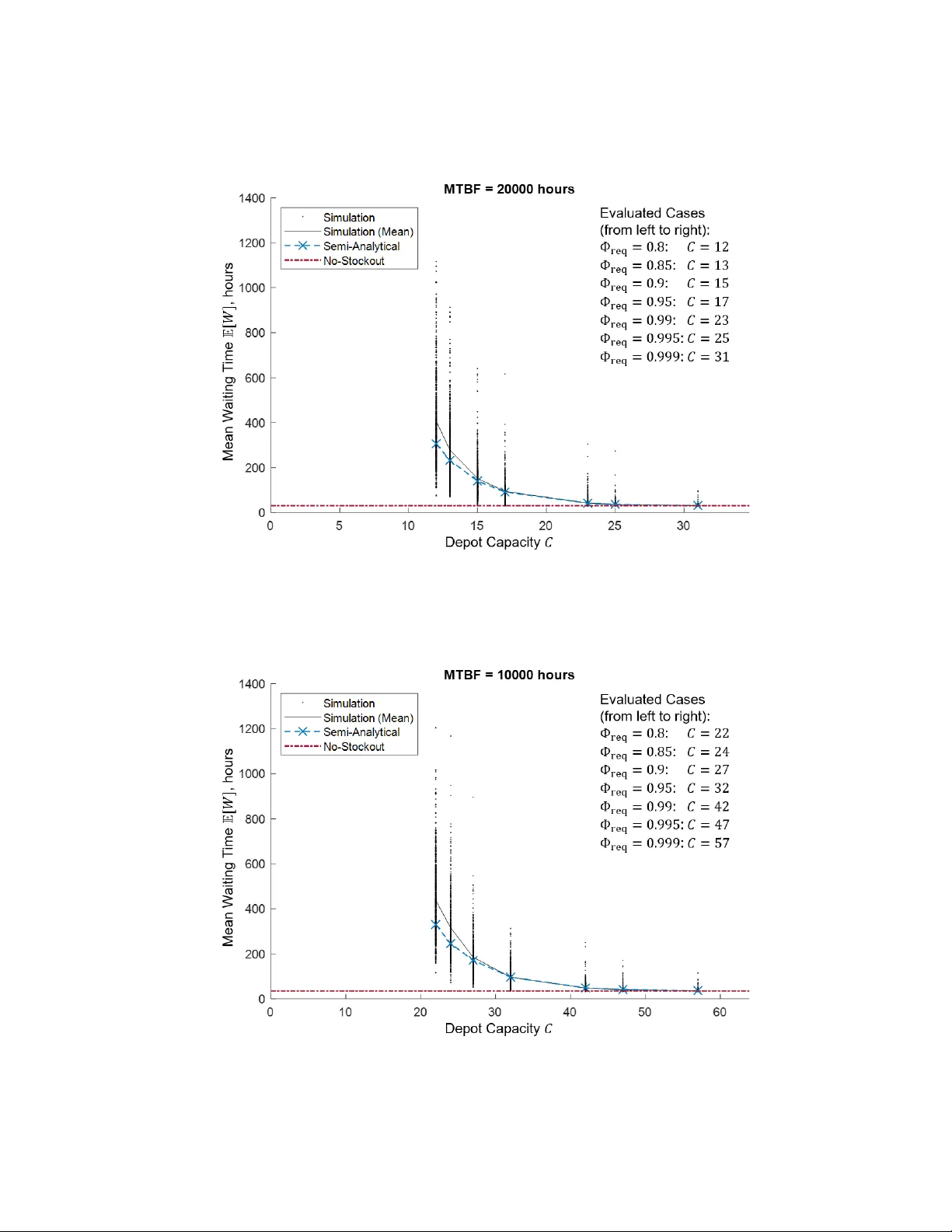
Semi- Anal ytical Model f or Design and Anal y sis of On-Orbit Servicing Ar chitectur e K oki Ho ∗ Georgia Ins titute of T ec hnology, Atlanta, GA, U .S.A. Hai W ang † Sing apore Manag ement U niver sity, Singapor e, Sing apor e Carnegie Mellon Univ ersity , Pittsburgh, P A, U .S.A. Paul A. DeT rempe ‡ Stanf ord Univ ersity , Stanf ord, CA, U.S.A. T r istan Sar ton du Jonchay § , and Kento T omita ¶ Georgia Institute of T echnology , Atlanta, GA, U .S.A. Robo tic on-orbit servicing (OOS) is expected to be a k e y technology and concept f or future sustainable space e xploration. This paper de velops a nov el semi-analytical model f or OOS system analy sis, responding to the gro wing needs and ongoing trend of robotic OOS. An OOS infrastructure system is considered whose goal is to pro vide responsiv e services to the random failures of a set of customer modular satellites distributed in space (e.g., at the geosynchr onous orbit). The considered OOS architectur e comprises a servicer that tra v els and pro vides module- replacement services to the customer satellites, an on-orbit depot to stor e the spares, and a series of launch v ehicles to replenish the depot. The OOS system performance is anal yzed b y ev aluating the mean w aiting time bef ore service com pletion f or a giv en failure and its relationship with the depot capacity . By uniquely lev eraging queueing theory and in v entory management methods, the dev eloped semi-analytical model is capable of analyzing the OOS system performance without relying on computationally costly simulations. The effectiv eness of the proposed model is demonstrated using a case study compared with simulation results. This paper is expected to pro vide a critical step to push the researc h frontier of analytical/semi- analytical model de v elopment f or comple x space systems design. Nomenclatur e ∗ Assistant Professor , Daniel Guggenheim School of Aerospace Engineering, Atlanta, GA, AIAA Senior Member † Assistant Professor , School of Inf ormation Sys tems, Singapore, Singapore; Visiting Assistant Prof essor, Heinz College of Information Sys tems and Public Policy , Pittsburgh, P A, U.S.A. ‡ M.S. Student, Depar tment of Aeronautics and Astronautics, Stanf ord, CA § Ph.D. Student, Daniel Guggenheim School of Aerospace Engineering, Atlanta, GA, AIAA Student Member ¶ Ph.D. Student, Daniel Guggenheim School of Aerospace Engineering, Atlanta, GA, AIAA Student Member C = on-orbit depot spare capacity , in units of modules D = spare demand, in units of modules per hour L = lead time, in units of hours N = number of customer satellite modules, in units of modules S = service time, in units of hours S inbound = inbound trav el time, in units of hours S outbound = outbound trav el time, in units of hours S repair = repair time, in units of hours S stoc kout = e xtra ser vice time due to stoc kout, in units of hours T l = launch inter v al, in units of hours T s = time until stock out, in units of hours W = waiting time until ser vice completion, in units of hours W q = waiting time in queue, in units of hours α = mean individual module failure rate, in units of f ailures per hour β = mean launch rate, in units of launches per hour λ = mean sys tem-lev el spare demand rate, in units of modules per hour Φ = fill rate Φ req = fill rate requirement f · = probability density function E [ · ] = e xpected value { L ∗ · } ( θ ) = Laplace-S tieltjes transf or m of a function I. Introduction No wada ys, there has been increasing interest in dev eloping on-orbit infrastr ucture systems that enable sustainable space exploration. Ov er the last sev eral decades, research and de v elopment in autonomous and robotics sys tems ha v e significantly raised the technology readiness le v el of robotic on-orbit servicing (OOS) [ 1 – 3 ]. Engineers en vision space-based servicing infrastr uctures to pro vide refueling and repair services or to manufacture larg e str uctures directl y in orbit. The recent trend of satellite modular ization is also enabling the concepts of “ser vicing-friendly” spacecraft that are composed of multiple small str uctural modules with standardized interface mechanisms [ 4 – 7 ]. These OOS infrastructure sys tems and ser viceable satellite designs are e xpected to be game-changing technologies for the satellite industry [8 – 12]. 2 T raditionally , most OOS concepts studied in the literature hav e assumed a dedicated robotic spacecraft to repair or refuel the customer satellites [ 13 – 15 ]. The ser vicer w ould visit a predefined set of satellites and be discarded once the mission is ov er . The advantag e of this concept is that the flight path of the ser vicer can be optimized before launch to pro vide the best value to the ser vice operation. Ho w ev er , although such a “disposable" ser vicer may be a fa v orable concept in the near ter m, it is not a sustainable solution f or OOS in the longer ter m. Alternativel y , a more sustainable concept is to use a per manent reusable ser vicing infrastructure that responds to random failures [ 11 , 16 ]. One e xample of such a concept would include a ser vicer replacing defectiv e modules with ne w module spares, an on-orbit depot stor ing the spare modules, and a ser ies of launch vehicles supplying new modules from Ear th to the depot on a regular basis. When a module fails on a satellite, the OOS system dispatches a ser vicer with a ne w spare to that satellite to replace the failed module with the spare. This concept can provide timely and responsive services to the random failures spontaneously and thus enable sustainable space exploration. Ho w ev er , despite the potential advantag e of a permanent responsiv e OOS infrastructure sys tem, its design and operations planning are substantiall y more complex and challenging compared with the traditional dedicated ser vicer concepts. This is because the analy sis of a responsive OOS sys tem would need to consider the interactions betw een the infrastructure elements as w ell as the full supply chain of the spare modules, including the queue of the ser vices and the in v entory of the spare depot. W e need an efficient model to analyze the design of such a comple x OOS sy stem. In response to this background, we dev elop a nov el semi-analytical model to e valuate the OOS sys tem design and anal ysis. Giv en a set of distr ibuted modular satellites (i.e., customer satellites) with random failure rates, the proposed model can analyze the performance of the ser vicing sys tem considering the spares’ supply chain. Specifically , it can ev aluate the mean waiting time bef ore ser vice completion for a given customer satellite failure and its tradeoff relationship with the depot capacity . The dev eloped semi-anal ytical model uniquel y lev erages queueing theory and inv entor y management methods. Queueing theor y is the mathematical theory of waiting in lines; it models real-wor ld queueing sys tems using distributions of customer ar rival, ser vice time, and queue discipline [ 17 ]. Inv entor y management refers to the process of order ing, storing, and using inv entor y , such as ra w materials, components, and end products; inv entor y control methods can be applied to find an order policy that balances in v entory cost and demand shor tage [ 18 ]. Based on these theor ies, the dev eloped model for the OOS system contains a set of coupled submodels: (1) a queueing submodel that models the mean waiting time before ser vice completion for a module failure; and (2) an inv entor y control submodel that models the replenishment of the on-orbit depot from the g round. The results from the semi-analytical model are compared with simulation results for different real-w orld cases, and the accuracy of the proposed model is demonstrated. A f e w remarks need to be made about the value and contr ibution of the semi-analytical model dev eloped in this paper . Con v entionally , the anal ysis of space sy stems with random failures and repairs (e.g., OOS systems) has been performed using computationally costly discrete-ev ent or ag ent-based simulations [ 11 , 13 , 16 , 19 – 21 ]. Ho w ev er , as space 3 sys tems become complex, designing and ev aluating their per f or mance using only simulations becomes computationally challenging. While simulations are effectiv e f or detailed design, there is a growing need f or the dev elopment of more efficient, yet r igorous, analy sis methods to enable quick per f or mance ev aluation for systems design and trade space e xploration. Although analytical or semi-analytical models hav e been recently introduced gradually in space systems design [ 22 , 23 ], this research direction remains largel y une xplored. This paper introduces the first semi-analytical approach with an integrated queueing and in v entory model f or comple x space systems analy sis. The dev eloped approach enables the e valuation of the OOS sys tem performance without relying on computationally costl y simulations, reducing the computational time from hours down to seconds. The model de v eloped in this paper is e xpected to be a cr itical step in pushing forward this research frontier of anal ytical/semi-analytical model dev elopment f or space sys tems design. The rest of the paper is org anized as f ollow s. Section II discusses the ov er vie w of the considered OOS architecture. Section III explains the main contr ibution of the work: a semi-analytical model f or the OOS system. Section IV assesses the results from the proposed model using simulations with a realistic application e xample, and Section V concludes the paper . II. Overvie w of On-Orbit Servicing Infrastructure This paper considers an OOS architecture to pro vide module-replacement ser vices to a set of customer satellites distributed in space (e.g., at the geosynchronous orbit). The customer satellites are modular , where each module can fail and be replaced independently . The servicing architecture comprises three main components: the servicer, the on-orbit depot, and the launch v ehicles. The on-orbit depot stores modules which are brought to customers by the ser vicer when f ailures (i.e., demand f or ser vices) happen. The launch v ehicles are used to refill the depot. An illustration of the considered ser vicing architecture is shown in Fig. 1. Fig. 1 Illustration of customer , servicer , and resupply architecture. The ov er vie w of the concept of operations is as f ollo ws. The ser vicer remains docked to the depot while a waiting a customer satellite module f ailure. Once a customer satellite module fails, the ser vicer per f or ms a maneuv er to the 4 failed module. After the rendezvous and docking with the customer satellite, the servicer per f or ms the repair operation, defined as the replacement of a failed module with a spare module, and then retur ns to the depot via another maneuver . Customers receiv e ser vices in the order in which the y failed. If a failure happens while the servicer is busy , it has to wait until the ser vicer becomes av ailable (i.e., completes all the previous services in the queue) to receiv e the ser vice. The servicer can only car r y one spare module, and thus it must retur n to the depot to load a new spare and, if needed, refuel itself prior to the ne xt repair trip. The spare inv entor y in the depot is monitored regularl y , and the launch v ehicle visits the depot for its resupply f ollowing a stochas tic launch schedule. III. Semi-Anal ytical Model This section provides an o verview of the problem statement, the details of the dev eloped model, and the proposed solution method based on the model. A. Problem Statement W e dev elop a no v el semi-anal ytical model to ev aluate the OOS system design and analy sis without relying on computationally costl y simulations. As the first step, this subsection conv er ts the concept of operations of the considered OOS system into a mathematical problem. The ov erall concept of operations can be expressed in a schematic diag ram in Fig. 2. Follo wing the architecture discussed in Section II, the model contains a set of customer satellite modules operated in orbit; when a failure happens to a module, it is added to the queue for ser vice operations and is processed on a first-come-first-serv ed (FCFS) basis. T o sustain the service operations, the depot is replenished from the ground regularl y . In this study , we consider all modules to be identical for simplicity , and the failures of each module are assumed to f ollo w a (mutuall y independent) Poisson process. Fig. 2 Schematic representation of the customer satellite modules and servicing architecture. 5 The queue f or the services needs to be analyzed r igorously to capture both the ser vice time and the waiting time. The service time is the time during which the ser vicer is dedicated to a ser vice operation (i.e., from the moment when the servicer becomes av ailable for a ser vice operation until it returns to the depot upon completion of that ser vice). The waiting time, on the other hand, is defined as the time that a customer satellite module failure (i.e., demand) has to wait until it is ser viced (i.e., from the moment when a failure happens until its repair service is completed by the ser vicer). Mathematically , we can define the service time S and the waiting time W as follo ws: S = S stoc kout + S outbound + S repair + S inbound (1) W = W q + S stoc kout + S outbound + S repair (2) where S stoc kout is the delay of the service when the depot is f ound to be out of stoc k ∗ ; S outbound and S inbound are the outbound and inbound (i.e., retur n) tra v el times; S repair is the repair time; and W q is the waiting time in the queue. Here, S outbound and S inbound can be f ound from the (kno wn) distribution of the positions of the customer satellites; these times can also include the time for the operations needed bef ore and/or after each repair tr ip (e.g., loading a new spare, refueling). S repair is assumed to be a fixed value in this paper but can be varied if needed. The ev aluation of the remaining terms requires an integ rated queueing and inv entor y control analy sis; S stoc kout is an output from the inv entor y control analy sis, and W q is an output from the queueing analy sis. Note that W q depends on the ser vice times of all the previous repairs in the queue, and the length of the queue itself is also probabilistic. This coupled relationship makes the problem challenging. The considered in v entor y control strategy of the depot can be modeled as a modified version of the order-up-to policy [ 24 ]. Namel y , o v er e v er y exponentiall y distributed time inter val T l ∼  ( β ) , we revie w the inv entor y and order C − ( I + I 0 ) units from the ground, where C is the capacity of the depot, I is the cur rent in v entor y lev el, and I 0 is the replenishment on the wa y (i.e., orders being processed). Here, the in v entor y lev el I is defined as the number of units ph ysicall y in stoc k minus the number of back orders, where the back orders are used to track the unmet demand due to stoc kout so that it can be deliv ered at subsequent oppor tunities. The revie w frequency is dr iv en b y the launch frequency of the rocket with a mean launch rate β . The exponential distribution f or the launch interval has been sho wn to be a good approximation; see Appendix of Ref. [ 22 ]. A constant lead time L is added between the revie w oppor tunity and the actual delivery of the spares in order to account f or the processing of the order , the manufacturing of the units, the loading of the units onto the rock et, and the flight time to the depot. Fig. 3 summar izes the considered in v entor y control policy . A ke y consideration f or the inv entor y per f or mance is the fill rate Φ , representing the percentage of the spare demand ∗ T echnically speaking, S stock out is not a service time, but w e consider it as par t of the service time so that the queueing and in ventory control methods can be coupled naturally . 6 Fig. 3 Order-up-to policy for the depot inv entory control. that is met without stock out. W e assume that w e are given a fill rate requirement Φ req (typically close to one), and our goal is to analyze the mean waiting time E [ W ] and the depot capacity C . The tradeoff between E [ W ] and C cor responds to a cost-perf or mance tradeoff. W e prefer a lo w-cos t and high-performance OOS sy stem, which can be inter preted as a sys tem with a small C and a small E [ W ] ; how ev er, as shown later , a smaller C typically indicates a larg er E [ W ] , and thus the tradeoff between these tw o needs to be considered. Particularl y , we are interested in the behavior of E [ W ] vs. C around the knee region of the cur ve † , which represents the depot capacity C abo v e which little additional saving is e xpected in the mean waiting time E [ W ] . In practice, this indicates the solution point bey ond which it is not worth in v esting more on e xpanding the depot capacity consider ing the small per f or mance gain (i.e., waiting time reduction); the definition of that e xact solution would depend on the cost model f or the depot and the (monetar y) penalty model f or the waiting time, both of which are application-dependent. In this paper , instead, w e aim to dev elop a general method to efficientl y ev aluate the solutions around that knee region rather than specifying the e xact point. This concept is sho wn in Fig. 4. Note that this knee region cor responds to where Φ req is close to one; therefore, in later numer ical examples, w e particularly f ocus on the solutions around Φ req = 0 . 95 or abov e, which is tr ue for a realistic reliable OOS sys tem. B. Proposed Model This subsection introduces the proposed model to analyze the performance of the OOS sys tem. The dev eloped model lev erages queueing theor y and in v entor y control methods; the integrated queueing and inv entor y model is † There are multiple definitions of the knee point/region in the multi-objective optimization literature [ 25 , 26 ]; in this paper, we use the concept of "the knee of the cur ve" to represent the region around the point of diminishing returns. 7 Fig. 4 Solutions around the knee region of the curv e of mean waiting time vs. depot capacity summarized in Fig. 5. The inputs to the model include the probability distributions of the trav el and repair times ( f S outbound , f S repair , f S inbound ), the individual module failure rate α , the number of modules N , the length of lead time L , the mean launch rate β , and the required fill rate Φ . The integrated queueing and inv entor y control model takes those inputs and derives the mean waiting time E [ W ] and the depot capacity C . The queueing and the inv entory control submodels interact as follo ws: the queueing submodel generates the spare demand (i.e., module failure) distribution f D , which is f ed into the in v entor y control submodel to calculate the probability distribution of the e xtra ser vicing time due to stoc k out f S stock out ; this distribution is fed back into the queueing submodel. Since it is difficult to analyticall y handle the spare demand distribution f D due to its state-dependent nature, we approximate this b y a P oisson process with the corresponding mean demand rate λ . In this wa y , f D can be characterized using onl y λ , which is par t of the output from the queueing submodel. (N ote that this value is not just the consolidation of the individual module failure rate α because the system failure rate is state-dependent; see Section III.B.1.) This approximation is demonstrated to per f or m w ell in later numer ical simulations. Fig. 5 Integrated queueing and in v entory model for the OOS system. The f ollowing subsubsections introduce the details of the queueing submodel and inv entory control submodel in the 8 integrated model as w ell as their mathematical coupling. 1. Queueing Submodel The queueing par t of the OOS problem can be modeled using a finite-source queue. A finite-source queue represents the case where the number of customer satellite modules is finite. Consequently , as the number of failed modules increases, the number of activ e modules decreases, thus decreasing the sys tem-lev el f ailure rate. This fact makes the f ailure rate state-dependent (i.e., the failure rate depends on the number of active modules), and thus makes the problem challenging. Using Kendall’ s notation [27, 28], the considered queue is wr itten as M / G / 1 / N / N (or M / G / 1 // N depending on the literature [29]). The meaning of each letter is as f ollo ws: • M : The ar rival process is Marko vian (Poisson process). • G : The service time distribution is general. • 1 : The number of servicers is one. • N : The number of failures allow ed in the queue is N . • N : The size of the source population is N . The general solution for the M / G / 1 / N / N queue can be f ound using the Laplace-Stieltjes transf or m of the ser vice time distribution. Denoting the Laplace-Stieltjes transf or m of a function f as { L ∗ f } ( θ ) , the mean spare demand rate λ becomes: λ = 1 − P 0 E [ S ] (3) where P 0 =  1 + N E [ S ] α N − 1  n = 0  N − 1 n  B n  − 1 (4) B n =            1 if n = 0  n i = 1  1 − { L ∗ f S } ( i α ) { L ∗ f S } ( i α )  if n = 1 , 2 , . . . , N − 1 (5) The mean waiting time E [ W ] is: E [ W ] = N λ − 1 α − E [ S inbound ] (6) The der ivation of the abo v e equations can be f ound in Ref s. [ 30 ] and [ 31 ] ‡ . Here, the mean and the probability distribution of the ser vice time, E [ S ] and f S , can be f ound using Eq. (1) , where the distributions of S outbound , S repair , and S inbound are known and the distribution of S stoc kout can be found using the inv entor y analy sis (see Eq. (12) ). Also, λ in ‡ The last term of Eq. (6) (i.e., the subtraction of E [ S inbound ] ) is added to accommodate our definition of the waiting time. 9 Eq. (3) is used to generate the demand distribution f D with a Poisson assumption as discussed abo v e: f D ( i ; λ , t ) = λ i t i e − λ t i ! (7) This f D is then fed into the in v entor y control analy sis. Note that an implicit assumption for this queueing analy sis is that, since the servicer’ s retur n tra v el time S inbound is included as par t of the ser vice time, the replaced module does not resume nor mal operation (i.e., module f ailure process does not restart) until the ser vicer retur ns to the depot after its ser vice. This appro ximation is reasonable in practice especially when the module’ s mean time between failures (MTBF) is sufficiently long, as demonstrated in the later comparison with simulations. 2. Inventory Control Submodel The inv entor y control analy sis f or the OOS problem contains tw o par ts: finding C given Φ req and finding f S stock out . For the order -up-to policy [24], the fill rate Φ is defined as f ollow s: Φ = 1 −  ∞ 0  ∞ i = 1 max ( 0 , i − C ) f D ( i ; λ , t + L ) f T l ( t ; β ) d t  ∞ 0  ∞ i = 1 i f D ( i ; λ , t ) f T l ( t ; β ) d t = 1 − β λ  ∞ 0 ∞  i = 1 max ( 0 , i − C ) f D ( i ; λ , t + L ) f T l ( t ; β ) d t (8) where the exponential launch inter val distribution is as f ollow s: f T l ( t ; β ) = β e − β t (9) and the demand distribution f D can be f ound in Eq. (7) . The numerator of the second ter m in Eq. (8) is the expected bac korder ov er a launch interval and a lead time , whereas the denominator is the expected demand ov er a launc h interval . The reason why the numerator considers both the launch interval and the lead time (instead of only the launch interval) can be intuitiv el y e xplained with the f ollo wing example. Consider a case where an order is made at a point when the in v entory lev el is I units, and there is no other replenishment order on the wa y . In this case, the order w ould be deliv ered after L time steps when the in v entory lev el is I − I L units, where I L is the additional units of demand during the lead time L . Because the order only delivers C − I units using the information when the order w as made, the actual in v entory r ight after the replenishment deliv er y is ( I − I L ) + ( C − I ) = C − I L instead of the full capacity C . Therefore, a stoc kout (and thus a back order) happens when the demand betw een this deliv er y and the ne xt deliv er y (i.e., o v er one launch inter val), denoted as I I , e xceeds C − I L ; this corresponds to when the summation of the demand o v er an interval ( I I ) and the demand ov er the lead time ( I L ) ex ceeds C . This e xplains why the fill rate computation needs to take into 10 consideration the back order o ver both the launch inter v al and the lead time. For a more r igorous derivation of the fill rate expression in Eq. (8), see R ef. [24]. A closed-form e xpression for Φ (Eq. (8)) can be der iv ed as f ollow s: Φ = 1 − β λ  ∞ 0 ∞  i = 1 max ( 0 , i − C ) f D ( i ; λ , t + L ) f T l ( t ; β ) d t = 1 − β λ  ∞ 0 ∞  i = 1 i β e − β t λ C + i ( t + L ) C + i e − λ ( t + L ) ( C + i ) ! d t = 1 − β λ       e − λ L  λ β + λ  C λ β C  j = 0 { ( β + λ ) L } j j ! + L λ      1 − e − λ L C − 1  j = 0 ( λ L ) j j !      +  λ β − C       1 − e − λ L C  j = 0 ( λ L ) j j !            This e xpression allow s us to ev aluate the fill rate Φ giv en a depot capacity C . With this e xpression, we can find the minimum C that satisfies a given fill rate requirement Φ req : min C (10) s.t. Φ ≥ Φ req (11) Since Φ is a monotonically increasing function of C , the solution to this problem can be f ound simply by iterativel y incrementing C until Φ ≥ Φ req is satisfied. Using the depot capacity C , we can der iv e the e xpression f or the additional service time due to stock out S stoc kout , which is then fed back to the queueing analy sis. S stoc kout corresponds to the extra "ser vice" time that the first repair finding the depot to be out of stock needs to wait before the ser vicer can depart for the repair ser vice. The impact of this e xtra ser vice time then propagates to the remaining repairs through their waiting times in the queue W q . T o der iv e the e xpression f or S stoc kout , we consider the f ollo wing two cases. If the time it takes to hav e C + 1 units of demand (i.e., f ailures), denoted as T s , is the same or longer than the sum of the launch interval and the lead time ( T l + L ), then no extra service time is added to the repairs in that inter val. If that is not the case ( T l + L > T s ), then w e add an extra ser vice time S stoc kout cor responding to T l + L − T s to the first unit of repair demand that finds the depot to be out of stock. Considering that only one out of λ 1 β units of repair demand on av erage in each launch inter val can potentiall y be affected, S stoc kout can be wr itten as f ollow s: S stoc kout =            max ( T l + L − T s , 0 ) with p = β λ 0 with p = 1 − β λ (12) where T l and T s themsel v es are also random variables follo wing the probability density functions f T l ( t ; β ) and f T s ( t ; λ , C + 1 ) , respectivel y . f T l ( t ; β ) can be f ound using Eq. (9) , and f T s ( t ; λ , C + 1 ) can be expressed with an Erlang 11 distribution because of the Poisson demand approximation: f T s ( t ; λ , C + 1 ) = λ C + 1 t C e − λ t C ! = f D ( C ; λ , t ) λ (13) Note that this is a conservativ e approximation; in reality , S stoc kout can be shorter because the impact of stock out does not take effect until all the ongoing repairs in the queue with the in-stoc k spares are completed. One comment about the assumption behind the inv entor y control submodel needs to be added: the considered model does not ha v e an upper limit on the number of units a rock et can car r y ev en when there are a larg e number of back orders; although w e ha v e a rocket capacity constraint in reality , this assumption is reasonable when the solutions are near the knee region, where a stoc kout happens rarely . In later simulations, a rock et capacity constraint up to C units is enforced, and the proposed model is demonstrated to approximate the simulation results w ell ne v er theless. 3. Coupling betw een the Queueing and Inv entor y Control Submodels W e next look at how the queueing submodel and the inv entor y control submodel are mathematically coupled. Firs t, we consider the queueing submodel and der iv e the e xpressions for λ and E [ W ] f or a given distribution of S stoc kout . Examining Eqs. (3) - (6) , w e can see that the only complication for this process is obtaining the e xpressions for E [ S ] and { L ∗ f S } ( θ ) . E [ S ] can be expressed as: E [ S ] = E [ S stoc kout ] + E [ S outbound ] + E  S repair  + E [ S inbound ] (14) Similarl y , lev eraging the con v olution theorem for the Laplace-Stieltjes transf orm, { L ∗ f S } ( θ ) can be expressed as: { L ∗ f S } ( θ ) =  L ∗ f S stock out  ( θ )  L ∗ f S outbound  ( θ )  L ∗ f S repair  ( θ )  L ∗ f S inbound  ( θ ) (15) The terms f or S outbound , S repair , and S inbound in Eqs. (14) - (15) can be der iv ed using orbital mechanics; der iving this analytical e xpression is trivial because we know the ex act locations of the customer satellites. Thus, if we are giv en the closed-f or m e xpressions f or E [ S stoc kout ] and  L ∗ f S stock out  ( θ ) from the inv entor y control submodel, λ and E [ W ] can be f ound analyticall y . Ne xt, we e xamine the ter ms f or S stoc kout in Eqs. (14) - (15) , E [ S stoc kout ] and  L ∗ f S stock out  ( θ ) , through the inv entor y control submodel. These ter ms can be analyticall y expressed using C (obtained from Eqs. (10) - (11) ) and λ . W e first derive  L ∗ f S stock out  ( θ ) and use that to find E [ S stoc kout ] .  L ∗ f S stock out  ( θ ) = β λ  L ∗ f max ( T l + L − T s , 0 )  ( θ ) +  1 − β λ  (16) 12 Focusing on  L ∗ f max ( T l + L − T s , 0 )  ( θ ) ,  L ∗ f max ( T l + L − T s , 0 )  ( θ ) =  ∞ 0   t l + L 0 e − θ ( t l + L − t s ) β e − β t l λ C + 1 t C s e − λ t s C ! d t s  d t l +  ∞ 0   ∞ t l + L β e − β t l λ C + 1 t C s e − λ t s C ! d t s  d t l = β β + θ  λ λ − θ  C + 1 e − θ L  1 − C  n = 0 e −( λ − θ ) L ( β + θ )( λ − θ ) n ( β + λ ) n + 1 n  i = 0 { ( β + λ ) L } i i !  + C  n = 0 e − λ L β λ n ( β + λ ) n + 1 n  i = 0 { ( β + λ ) L } i i ! (17) Thus, we hav e obtained a closed-f or m e xpression f or  L ∗ f S stock out  ( θ ) . Using  L ∗ f S stock out  ( θ ) , E [ S stoc kout ] can be f ound as f ollo ws: E [ S stoc kout ] = − d d θ  L ∗ f S stock out  ( θ ) | θ = 0 = β λ  L + 1 β − C + 1 λ + C  n = 0 ( C + 1 − n ) e − λ L β λ n − 1 ( β + λ ) n + 1 n  i = 0 { ( β + λ ) L } i i !  (18) As we can see in the resulting expressions, the ter ms needed for the expressions of λ and E [ W ] depend on the distribution of S stoc kout (i.e., through the queueing analy sis), and this distr ibution of S stoc kout depends on λ (i.e., through the inv entor y control analy sis). Theref ore, this sys tem of equations needs to be solv ed concur rently § . C. Solution Method With the proposed coupled queueing and inv entor y control submodels, our goal is to find the solution of the mean waiting time E [ W ] and the depot capacity C f or a giv en fill rate requirement Φ req that is close to one (i.e., around the knee region of the E [ W ] vs. C curve). The coupled equations f or these two submodels generall y cannot be solv ed fully analyticall y; a standard numer ical solv er such as the fsolve function in MA TLAB can be lev eraged. The solution of these coupled equations enables us to find both E [ W ] (i.e., from the queueing analy sis) and C (i.e., from the inv entor y analy sis) f or a given Φ req . The performance of solving a set of coupled equations depends on the initial value. As the initial value f or solving our problem, we propose to use the no-stoc k out case, i.e., b y setting S stoc kout = 0 . In this case, f S stock out is not needed for the queueing analy sis, and theref ore the loop between the queueing and inv entor y control submodels is decoupled. Thus, w e can independently find the mean w aiting time E [ W ] and mean demand rate λ via Eqs. (3) - (6) . For highly reliable realistic OOS applications (i.e., Φ req ≈ 1 ), this solution is e xpected to be close from the tr ue solution, and thus ser v es as § A comment on the practical implementation: some ter ms in the der iv ed equations can span many orders of magnitude (e.g., the first ter m of Eq. (17) ), which can potentially cause numer ical instability . One technique to av oid such an issue is to implement the multiplications in those terms as additions in the log-domain. 13 a good initial value for the fsolve function. IV . Application Example This section applies the proposed method to an example case with realistic parameters and assesses the accuracy of the proposed model with simulations. The considered example case contains 10 customer satellites with 5 modules each that are ev enly distributed ov er the g eosynchronous orbit, and the depot is collocated with one of these satellites. The outbound and inbound trav el times are computed based on the phasing maneuv er between the depot and the satellite with the failed module, and the operations needed betw een each repair tr ip (e.g., loading a new spare, refueling) are assumed to be near -instantaneous ¶ . See Appendix f or the specific phasing maneuver strategy chosen in this e xample. The values of the ke y parameters are listed in T able 1. Three cases f or the module MTBF are considered. T able 1 Simulation Parameters. MTBF stands for the mean time between failures. Parameter V alue Repair time S repair 4 hours Launch lead time L 2160 hours Mean launch inter v al 1 / β 1213.4 hours MTBF per module 1 / α 20000, 10000, 4000 hours For the considered application case, the dev eloped semi-anal ytical model is used to derive the mean w aiting time vs. depot capacity cur ve ‖ . T o assess the accuracy of the proposed semi-analytical model, we use the depot capacity derived from the analy sis and ev aluate the cor responding waiting time of the system via simulations; the mean w aiting time results from the simulations are compared with those from the semi-analytical model. For each giv en set of the MTBF and the depot capacity , 500 simulation r uns are per f ormed ov er a time horizon of 200000 hours (i.e., ∼ 22 . 8 y ears). The simulation methods used in this paper are based on Ref. [ 16 ]. As discussed previousl y , to reflect the reality , the simulations enf orce a rock et capacity constraint that prev ents the replenishment rock et from delivering more units than the depot capacity ev en when there are back orders. W e ev aluate the cases with fill rate requirements Φ req = 0 . 8 , 0 . 85 , 0 . 9 , 0 . 95 , 0 . 99 , 0 . 995 , 0 . 999 , and expect the proposed model to perform well (i.e., approximate the simulation results accurately) when Φ req is close to one. The results of the semi-analytical model and the simulations are shown in Figs. 6-8. For the simulation results, the av eraged waiting times o v er the time hor izon for each 200000-hour r un are ev aluated f or the cor responding depot capacities and are sho wn as individual black dots in Figs. 6-8; additionall y , their means o v er the 500 simulations f or each depot capacity are connected b y a black solid line. The semi-analytical results for each fill rate are sho wn as ¶ The spare loading and refueling operations are assumed as near-ins tantaneous while the repair operations are not because the f ormer are generall y routine operations with a cooperativ e target (i.e., depot), whereas the latter include additional dedicated and inv olv ed operations with a non-cooperativ e target (i.e., failed customer satellites). This assumption can be easily relaxed by including additional cor responding service times. ‖ For this illustrativ e example, the fsolve function in MATLAB is used with the function tolerance of 10 − 4 , the optimality tolerance of 10 − 4 , and the step tolerance of 10 − 4 . 14 crosses connected by a blue dashed line in Figs. 6-8. In addition, w e derive the mean waiting time with no stoc kout (i.e., infinite capacity), shown as a horizontal red dash-dot line in Figs. 6-8. Fig. 6 Mean w aiting time vs. depot capacity f or mean time betw een f ailure = 20000 hours. The cases with various fill rate requirements Φ req = 0 . 8 , 0 . 85 , 0 . 9 , 0 . 95 , 0 . 99 , 0 . 995 , 0 . 999 are shown (from left to right) as crosses. The no-stock out case is also sho wn f or ref erence. Fig. 7 Mean w aiting time vs. depot capacity f or mean time betw een f ailure = 10000 hours. The cases with various fill rate requirements Φ req = 0 . 8 , 0 . 85 , 0 . 9 , 0 . 95 , 0 . 99 , 0 . 995 , 0 . 999 are shown (from left to right) as crosses. The no-stock out case is also sho wn f or ref erence. 15 Fig. 8 Mean waiting time vs. depot capacity for mean time betw een failur e = 4000 hours. The cases with various fill rate requirements Φ req = 0 . 8 , 0 . 85 , 0 . 9 , 0 . 95 , 0 . 99 , 0 . 995 , 0 . 999 are shown (from left to right) as crosses. The no-stock out case is also sho wn f or ref erence. The quantitative comparison of the results from the model and simulations is also sho wn in T able 2. Note that the er ror betw een the model and the simulations is caused b y both the approximation made in the model and the randomness in the simulations due to the finite number of r uns. From the results, w e can observe that the proposed method explores the relationship betw een the mean waiting time and the depot capacity around the knee region. Its e valuation of the mean waiting time achie v es an accuracy of < 5% when Φ req ≥ 0 . 95 . Note that, in practice, the OOS sy stem w ould be designed to ha v e a high fill rate (i.e. Φ req ≥ 0 . 95 ) in order to achie v e reasonable waiting times f or ser vice; therefore, the approximation in the dev eloped model ser ves a purpose. Additionall y , we can also obser v e that the no-stoc kout solution ser v es as an optimistic low er bound on the mean w aiting time. This no-stock out case cor responds to an ideal OOS system with infinite depot capacity and can be used as a first-order approximation of the mean waiting time. Overall, the results demonstrate the accuracy and utility of the proposed semi-analytical model for the considered OOS application. One benefit of the proposed model is that it does not require computationally costly simulations f or ev aluation. For the considered e xample, the simulations take more than 15 hours to complete the ev aluation of all cases with Python 3.6, whereas the semi-analytical model only takes approximatel y 5 seconds in total with MA TLAB R2019a ∗∗ . Although the e xact computational time depends on the implementation details, the substantial computational cost sa ving pro vided b y the de v eloped model is e vident. The dev eloped model provides an efficient high-lev el design anal ysis and optimization ∗∗ All tests w ere per f ormed on an Intel Core i7-8650U CPU @ 1.90GHz platf orm with 16GB RAM. 16 T able 2 Comparison between the semi-analytical results W semi-analytical and the simulation results W simulation . The no-stock out mean waiting time is also included for ref erence. The error in E [ W ] is ev aluated as    E  W semi-analytical  − E [ W simulation ]  / E [ W simulation ]   . MTBF , hours Φ req C E  W semi-analytical  hours E [ W simulation ] , hours Er ror in E [ W ] 20000 0.8 12 306.1 406.4 24.7% 0.85 13 232.1 278.5 16.7% 0.9 15 140.5 151.9 7.5% 0.95 17 91.5 94.2 2.9% 0.99 23 41.3 42.1 2.0% 0.995 25 36.6 36.6 0.0% 0.999 31 31.6 31.4 0.8% no-stoc k out – 30.5 – – 10000 0.8 22 330.1 437.9 24.6% 0.85 24 245.7 315.9 22.2% 0.9 27 171.3 185.0 7.4% 0.95 32 96.6 96.0 0.5% 0.99 42 48.4 47.5 1.8% 0.995 47 41.4 40.9 1.4% 0.999 57 36.8 36.5 0.6% no-stoc k out – 35.5 – – 4000 0.8 48 449.4 603.9 25.6% 0.85 54 323.5 399.9 19.1% 0.9 61 233.6 271.6 14.0% 0.95 73 143.4 149.7 4.2% 0.99 98 81.7 81.0 0.9% 0.995 109 73.5 72.9 0.8% 0.999 134 67.2 68.8 2.3% no-stoc k out – 65.8 – – method with sufficient accuracy for early -stag e sy stems design, complementing the e xisting costl y simulation techniques f or detailed design. V . Conclusion This paper dev elops a no v el semi-anal ytical model f or OOS sys tem analy sis based on queueing theory and inv entor y management methods. W e consider an OOS system that provides responsive ser vices to the random failures of a number of modular customer satellites in orbit. The considered OOS architecture comprises a servicer that pro vides module-replacement services to the customer satellites, an on-orbit depot that stores the spare modules, and a ser ies of launch vehicles to refill the depot. The dev eloped model is capable of analyzing the queue of the ser vice operations as w ell as the logistics of the spares, ev aluating the mean waiting time bef ore ser vice completion f or a given failure and its relationship with the depot capacity . The case study show s that the results from the semi-analytical model approximate 17 the solution well without computationally costl y simulations. Although this paper uses a simple OOS application case to demonstrate the v alue of the dev eloped model, the dev eloped general approach can be applied to more comple x OOS problems with reasonable modifications. Possible e xtensions include: (1) emplo ying a ser vicer that can carr y multiple spares (i.e., servicing multiple customers in one tr ip); (2) consider ing multiple types of spares, repair operations, or ev en ser vicer spacecraft; and (3) applying alternative inv entor y control policies for the depot. W e expect that this paper opens up a broad range of applications of semi-analytical models to OOS system design. A ckno wledgment The authors thank Br ian Hardy for running the simulations needed f or this paper and Hang W oon Lee and Onalli Gunasekara for revie wing this paper . Funding Sources This w ork is par tially suppor ted by the Defense Adv anced Researc h Projects Ag ency (D ARP A) Y oung F aculty A ward D19AP00127. The content of this paper does not necessar ily reflect the position or the policy of the U .S. Go v er nment, and no official endorsement should be inferred. Approv ed f or public release; distribution is unlimited. Appendix: Assump tion on Phasing Maneuv er in the Application Example This appendix summar izes the assumption on the phasing maneuv ers at the g eosynchronous orbit used in the e xample in this paper . Note that although this par ticular maneuv er strategy is chosen as an ex ample, the proposed method is compatible with other maneuv er strategies as well. The trav el time f or each phasing maneuv er o ver an angular separation ∆Θ (defined as the initial phasing angle of the servicer with respect to the targ et) at a circular orbit of radius r targ et ( ∼ 42160 km in the case of the geosync hronous orbit) is deter mined in the f ollowing wa y . W e first define two integer parameters k 1 ≥ 1 and k 2 ≥ 0 , where k 1 is the number of orbits the ser vicer tra v els in the phasing orbit and k 2 is the number of orbits the targ et trav els in its circular orbit before the rendezv ous. Using the definition of k 2 , the trav el time can be e xpressed as: t trav el = ( ∆Θ + 2 π k 2 )  r 3 targ et G M E (19) where G is the univ ersal gravitational constant and M E is the mass of the Ear th. Fur ther more, using the definition of k 1 , w e can find the relationship between the tra v el time and the semimajor axis of the phasing orbit a : t trav el = 2 π k 1  a 3 G M E (20) 18 Combining Eqs. (19)-(20) to an e xpression f or a using k 1 and k 2 : a =  ∆Θ + 2 π k 2 2 π k 1  2 3 r targ et (21) In the considered e xample, the values of k 1 and k 2 are chosen so that they minimize the tra v el time while satisfying the follo wing requirement: a ≥ r targ et + R E + h crit 2 (22) where R E is the radius of the Earth, and h crit is the minimum altitude f or the phasing orbit. In the numer ical example, h crit = 10000 km is used. This minimum altitude is applied to ensure minimum inter f erence of the servicer with the en vironment at lo w er orbits (e.g., atmospheric drag, orbital debr is, other satellites). N ote that the minimum tra v el time indicates the minimum f easible k 2 according to Eq. (19) ; theref ore, our goal is equiv alent to finding the minimum possible integer k 2 ≥ 0 that yields a f easible integer k 1 ≥ 1 with respect to the constraint in Eq. (22) . Such a solution can be found by using a simple iterative process. Ref erences [1] “NAS A Satellite servicing projects division, ” https://sspd.gsfc.nasa.gov/ , [Accessed 8/22/2019]. [2] “J AXA Manipulator flight demonstration, ” http://iss.jaxa.jp/shuttle/flight/mfd/index_e.html , [A ccessed 8/22/2019]. [3] “D ARP A R obotic servicing of g eosynchronous satellites (RSGS), ” http://www.darpa.mil/program/robotic- servicing- of- geosynchronous- satellites , [Accessed 8/22/2019]. [4] Sullivan, B., and Akin, D., “A sur v ey of serviceable spacecraft failures, ” AIAA Space 2001 Conf erence and Exposition , American Institute of Aeronautics and Astronautics, Res ton, Virigina, 2001. doi:10.2514/6.2001- 4540. [5] Hill, L., Barnhar t, D., Fo w ler , E., Hunter , R., Hoag, L. M., Sullivan, B., and Will, P ., “The Market f or Satellite Cellular ization: A historical view of the impact of the satlet mor phology on the space industry, ” AIAA SP A CE 2013 Confer ence and Exposition , American Institute of Aeronautics and Astronautics, Res ton, Virginia, 2013. doi:10.2514/6.2013- 5486. [6] Kerzhner , A. A., Ingham, M. D., Khan, M. O., Ramirez, J., De Luis, J., Hollman, J., Arestie, S., and Sternberg, D., “Architecting Cellularized Space Systems using Model-Based Design Exploration, ” AIAA SP A CE 2013 Conf erence and Exposition , American Institute of Aeronautics and Astronautics, Res ton, Virginia, 2013. doi:10.2514/ 6.2013- 5371. [7] Jaeger , T ., and Mirczak, W ., “Satlets - The Building Blocks of Future Satellites - And Which Mold Do Y ou Use?” AIAA SP A CE 2013 Conf erence and Exposition , Amer ican Institute of A eronautics and Astronautics, Res ton, Virginia, 2013. doi:10.2514/6.2013- 5485. 19 [8] Saleh, J. H., Lamassoure, E., and Hastings, D. E., “Space Systems Flexibility Provided by On-Orbit Servicing: Part 1, ” Journal of Spacecraft and Roc kets , V ol. 39, No. 4, 2002, pp. 551–560. doi:10.2514/2.3844. [9] Lamassoure, E., Saleh, J. H., and Hastings, D. E., “Space Systems Flexibility Provided by On-Orbit Servicing: Part 2, ” Journal of Spacecraft and Roc kets , V ol. 39, No. 4, 2002, pp. 561–570. doi:10.2514/2.3845. [10] Saleh, J. H., Lamassoure, E. S., Hastings, D. E., and Ne wman, D. J., “Fle xibility and the V alue of On-Orbit Ser vicing: New Customer -Centric Perspectiv e, ” Jour nal of Spacecraft and Rocke ts , V ol. 40, No. 2, 2003, pp. 279–291. doi:10.2514/2.3944. [11] Long, A., Richards, M., and Hastings, D. E., “On-Orbit Ser vicing: A Ne w V alue Proposition f or Satellite Design and Operation, ” Journal of Spacecraft and Roc kets , V ol. 44, No. 4, 2007, pp. 964–976. doi:10.2514/ 1.27117. [12] Saleh, J. H., “W eaving time into system architecture: new perspectives on flexibility , spacecraft design lifetime, and on-orbit servicing, ” Ph.D. thesis, Massachusetts Institute of T echnology , 2001. [13] Y ao, W ., Chen, X., Huang, Y ., and van T ooren, M., “On-orbit servicing system assessment and optimization methods based on lifecy cle simulation under mixed aleatory and epistemic uncer tainties, ” Acta Astronautica , V ol. 87, 2013, pp. 107–126. doi:10.1016/j.actaastro.2013.02.005. [14] Zhao, S., Gur fil, P ., and Zhang, J., “Optimal ser vicing of geostationary satellites considering ear th ’ s tr iaxiality and lunisolar effects, ” Journal of Guidance, Control, and Dynamics , V ol. 39, 2016, pp. 2219–2231. doi:10.2514/ 1.G001424. [15] V erstraete, A. W ., Anderson, D., St. Louis, N. M., and Jennif er , H., “Geosynchronous Earth Orbit Robotic Ser vicer Mission Design, ” Journal of Spacecraft and Rocke ts , V ol. 55, 2018, pp. 1444–1452. doi:10.2514/ 1.A33945. [16] Sarton du Joncha y, T ., and Ho, K., “Quantification of the responsiv eness of on-orbit servicing infrastructure f or modular ized earth- orbiting platf or ms, ” Acta Astr onautica , V ol. 132, No. A ugust 2016, 2017, pp. 192–203. doi:10.1016/j.actaastro.2016.12.021. [17] Larson, R. C., and Odoni, A. R., U rban Operations Resear ch , Dynamic Ideas, 2007. [18] Simchi-Le vi, D., Chen, X., and Bramel, J., The Logic of Logistics: Theor y , Algorithms, and Applications for Logistics Manag ement , Spr inger , 2014. [19] Baldesarra, M., “A Decision-Making Frame w ork to Deter mine the V alue of On-Orbit Servicing Compared to R eplacement of Space T elescopes, ” , 2007. [20] Richards, M., Shah, N., and Hastings, D., “ Agent Model of On-Orbit Ser vicing Based on Orbital T ransfers, ” AIAA SP A CE Conf erence and Exposition , 2007. doi:10.2514/ 6.2007- 6115. [21] Sears, P ., and Ho, K., “Impact Evaluation of In-Space Additiv e Manufacturing and Recy cling T echnologies f or On-Orbit Servicing, ” Journal of Spacecraft and Roc kets , V ol. 56, No. 6, 2018, pp. 1498–1508. doi:10.2514/1.A34135. [22] Jak ob, P ., Shimizu, S., Y oshikaw a, S., and Ho, K., “Optimal Satellite Constellation Spare Strategy Using Multi-Echelon In ventory Control, ” Journal of Spacecraft and Rocke ts , V ol. 56, No. 5, 2019. doi:10.2514/1.A34387. 20 [23] Chen, Z., Chen, H., and Ho, K., “ Analytical Optimization Method for Space Logistics, ” Jour nal of Spacecr af t and Roc kets , V ol. 55, No. 6, 2018, pp. 1582–1586. doi:10.2514/1.A34159. [24] Cachon, G. P ., and T er wiesch, C., Matc hing Supply with Demand: An Introduction to Operations Management , 3 rd ed., McGra w-Hill Education, 2012. doi:10.2307/1271510. [25] Das, I., “On characterizing the “knee” of the Pareto cur ve based on Normal-Boundar y Intersection, ” Structural Optimization , V ol. 18, 1999, pp. 107–115. doi:10.1007/ BF01195985. [26] Sudeng, S., and W attanapongsakorn, N., “Finding Knee Solutions in Multi-Objectiv e Optimization Using Extended Angle Dominance Approach, ” Information Science and Applications , edited b y K. J. Kim, Springer Berlin Heidelberg, Berlin, Heidelberg, 2015, pp. 673–679. doi:10.1007/978- 3- 662- 46578- 3_79. [27] Kendall, D. G., “Stochas tic Processes Occur r ing in the Theory of Queues and their Analy sis by the Method of the Imbedded Mark ov Chain, ” The Annals of Mathematical Statistics , V ol. 24, No. 3, 1953. doi:10.1214/ aoms/1177728975. [28] Lee, A. M., Applied Queueing Theor y , MacMillan, Ne w Y ork, NY , 1966. [29] Sztrik, J., “Queueing theor y and its Applications, a personal vie w, ” Proceedings of the 8th International Conf erence on Applied Inf ormatics , 2010. [30] T akács, L., Introduction to the Theor y of Queues , Oxf ord Univ ersity Press, Ne w Y ork, NY , 1962. [31] Gupta, U . C., and Rao, T . S. S. S. V ., “A recursive method to compute the steady state probabilities of the machine inter f erence model: (M/G/1) K, ” Computers and Operations Resear c h , V ol. 21, No. 6, 1994, pp. 597–605. doi:10.1016/0305- 0548(94)90075- 2. 21