Learning How to Listen: A Temporal-Frequential Attention Model for Sound Event Detection

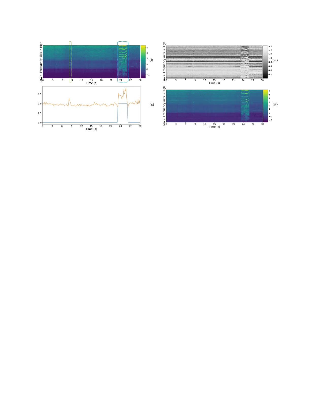
LEARNING HO W TO LISTEN: A TEMPORAL-FREQ UENTIAL A TTENTION MODEL FOR SOUND EVENT DETECTION Y u-Han Shen, K e-Xin He, W ei-Qiang Zhang Department of Electronic Engineering, Tsinghua Uni versity , Beijing, China yhshen@hotmail.com, hekexinchn@163.com, wqzhang@tsinghua.edu.cn ABSTRA CT In this paper, we propose a temporal-frequential attention model for sound ev ent detection (SED). Our network learns how to listen with two attention models: a temporal attention model and a frequential attention model. Proposed system learns when to listen using the temporal attention model while it learns where to listen on the frequency axis using the frequential attention model. W ith these two models, we attempt to make our system pay more attention to important frames or segments and important frequency components for sound event detection. Our proposed method is demonstrated on the task 2 of Detection and Classification of Acoustic Scenes and Events (DCASE) 2017 Challenge and achieves competiti ve performance. Index T erms — sound e vent detection, con volutional neural network, recurrent neural network, attent ion model, temporal- frequential attention 1. INTRODUCTION Now adays, sound ev ent detection (SED), also named as acoustic ev ent detection(AED), is considered as a popular topic in the field of acoustic signal processing. The aim of SED is to temporally locate the onset and offset times of target sound ev ents present in an audio recording. The Detection and Classification of Acoustic Scenes and Events (DCASE) Challenge is an international challenge concerning SED, and has been held for several years. In DCASE 2017 Challenge, the theme of task 2 is “detection of rare sound e vents” [1]. It provides dataset [2] and baseline for rare sound ev ent detection in synthesized recordings. Here, “rare” means that target sound events (babycry , glassbreak, gunshot) would occur at most once within a 30-second recording. And the mean duration of target sound event is very short: 2.25 s for babycry , 1.16 s for glassbreak, 1.32 s for gunshot, leading to a serious problem of data imbalance. All audio recordings are notated with ground-truth labels of e vent class, onset and offset time. According to the task description, a separate system should be developed for each of the three target event classes to detect the temporal occurrences of these ev ents [1]. Among the submissions in DCASE 2017, most models are based on deep neural networks. Both of the top 2 teams [3, 4] utilized Conv olutional Recurrent Neural Networks (CRNN) as their main architecture. They combined Conv olutional Neural Networks (CNN) with Recurrent Neural Networks (RNN) to make frame-le vel predictions for tar get ev ents and then adopted post-processing to get the onset and offset time of sound ev ents. Kao et al. [5] proposed a Region-based Conv olutional Recurrent Neural Network (R-CRNN) The corresponding author is W ei-Qiang Zhang. to improve previous work in 2018. In our work, we followed the main architecture of those three models and used CRNN as main classifier . Inspired by the excellent performance of attention model in machine translation [6], image caption [7], speaker verification [8], audio tagging [9], we proposed an attention model for SED. Cur- rently , most attention models in speech and audio processing only concentrate on time domain. W e proposed a temporal-frequential attention model to focus on important frequency components as well as important frames or segments. Our attention model can learn ho w to listen by e xtracting not only temporal information b ut also spectral information. Besides, we visualized the weights of attention models to show what our models ha ve actually learnt. The rest of this paper is organized as follows: in Section 2, we introduce our methods in detail, mainly including feature extraction, baseline and temporal-frequential attention model. The dataset, experiment setup and ev aluation metric are illustrated in Section 3. The results and analysis are presented in Section 4. Finally , we conclude our work in Section 5. 2. METHODS 2.1. System ov erview As shown in Figure 1, our proposed system is a CRNN architecture with temporal-frequential attention model. The input of our system is a 2-dim acoustic feature. It is fed into a frequential attention model to produce frequential attention weights. Our system learns to focus on specific frequency components of audios using those attention weights. The input acoustic feature will multiply with those attention weights and then pass through CRNN architecture. Compared with traditional CRNN [3, 4], we add a temporal attention model to let our system pay different attention to different frames. The temporal attention weights will multiply with the outputs of CRNN by element-wise. A sigmoid activ ation is used to get normalized probabilities. Then we utilize post processing to get final detection outputs. 2.2. Feature extraction The acoustic feature used in our work is log filter bank energy (Fbank). The sampling rate of input audios is 44.1kHz. T o e xtract Fbank feature, each audio is divided into frames of 40 ms duration with shifts of 20 ms. Then we apply 128 mel-scale filters cov ering the frequency range 300 to 22050 Hz on the magnitude spectrum of each frame. Finally , we take logarithm on the amplitude and get Fbank feature. The extracted Fbank feature is normalized to zero mean and unit standard de viation before being fed into neural networks. Fig. 1 . Illustration of overall system. 2.3. Baseline W e adopt state-of-the-art CRNN as baseline. The input is Fbank feature of 30-second audios. And the output of our system gi ves binary predictions for each segment with time resolution of 80 ms (4 times of the input frame shift 20 ms). The CRNN architecture consists of three parts: con volutional neural network (CNN), recurrent neural network (RNN) and fully- connected layer . The architecture of our CRNN is similar to that in [5], and it is shown in Figure 2. The CNN part contains four conv olutional layers, and each layer is followed by batch normalization [10], ReLU activ ation unit and dropout layer [11]. W e add two residual connections [12] to impro ve the performance of CNN. Max-pooling layers (on both time axis and frequency axis) are used to maintain the most important information on each feature map. At the end of CNN, the extracted features over different con volutional channels are stacked along the frequency axis. The RNN part is a bi-directional gated recurrent unit (bi-GRU) layer . Compared with uni-directional GR U, bi-GRU can e xtract temporal structures of sound events better . W e add the outputs of forward GRU and backward GR U to get final outputs of bi-GR U. The size of the output of bi-GR U is (375, U ), where U is the number of GR U units. After the bi-GR U, a single fully-connected layer with sigmoid activ ation is used to give classification result for each segment (4 frames). The output denotes the presence probabilities of the target ev ent in each segment. In order to determine the presence of an event, a binary predic- tion is given for each segment with a constant threshold of 0.5. These predictions are post-processed with a median filter of length 240 ms. Since at most one event would occur in a 30-s audio, we select the longest continuous sequence of positive predictions to get the onset and offset of tar get events. 2.4. Learning when to listen As sho wn in Figure 1, we add a temporal attention model at the end of CNN to enable our system to learn when to listen. This attention model was proposed to ignore irrelev ant sounds and focus Fig. 2 . The architecture of CRNN. The first and second dimensions of con volutional k ernels and strides represent the time axis and frequency axis respecti vely . more on important segments. Unlike the attention model in audio classification [9] that only focuses on positi ve segments (including ev ents), our temporal attention pays more attention to both positive segments and hard negati ve segments (only backgrounds, but easily misclassified as events) because they should be further dif ferentiated. The output of CNN will pass through a fully-connected layer with N t hidden units, followed by an activ ation unit (sigmoid, ReLU, or softmax). Then a global max-pooling on the frequency axis is used to get one weight for each segment. Those attention weights will be normalized along time axis. In our experiments, this operation of normalization has shown great effecti veness because it takes into account the variation of weight factors along time axis instead of considering only current segment. Then we multiply the temporal attention weights with the output of the fully-connected layer after bi-GRU. A sigmoid function is used to normalize the probabilities to [0 , 1] . The final output can be computed as follo ws: ˆ a t = max n ∈{ 1 , 2 , 3 ,...,N t } { σ ( W n C t + b n ) } , (1) a t = T ˆ a t P t ˆ a t , (2) y t = 1 1 + exp( − a t h t ) , (3) where σ ( · ) is an activ ation function, C t denotes the output of CNN, W n and b n represent the weights and bias for the n -th hidden unit respectiv ely , n ∈ { 1 , 2 , 3 , . . . , N t } and N t is the number of hidden units in time attention model. ˆ a t is the candidate temporal attention weight, T is the total number of segments in an audio, a t is the normalized temporal attention weight, and y t is the final output probabilities. 2.5. Learning where to listen Apart from temporal attention model, we proposed a frequential attention model. As we all know , various sound events may have different spectral characteristics. So we assume that we should treat T able 1 . Performance of proposed models and other methods, in terms of ER and F-score (%). *** indicates that class-wise results are not giv en in related paper . W e compare the following models: (1) Baseline: our bi-GR U-based CRNN; (2) CRNN+T A: our bi-GRU-based CRNN with temporal attention model; (3) Proposed: our bi-GRU-based CRNN with temporal-frequential attention model; (4) R-CRNN: Region-based CRNN; (5) 1d-CRNN: DCASE 1st place model; (6) CRNN: DCASE 2nd place model. Model Dev elopment Dataset Evaluation Dataset babycry glassbreak gunshot av erage babycry glassbreak gunshot average Baseline 0.14 | 92.6 0.04 | 98.0 0.19 | 89.6 0.12 | 93.4 0.31 | 83.4 0.08 | 95.9 0.26 | 85.5 0.22 | 88.3 CRNN+T A 0.14 | 92.8 0.03 | 98.4 0.17 | 90.9 0.11 | 94.0 0.25 | 87.4 0.05 | 97.4 0.18 | 90.6 0.16 | 91.8 Proposed 0.10 | 95.1 0.01 | 99.4 0.16 | 91.5 0.09 | 95.3 0.18 | 91.3 0.04 | 98.2 0.17 | 90.8 0.13 | 93.4 R-CRNN [5] 0.09 | *** 0.04 | *** 0.14 | *** 0.09 | 95.5 ****** ****** ****** 0.23 | 87.9 1d-CRNN [3] 0.05 | 97.6 0.01 | 99.6 0.16 | 91.6 0.07 | 96.3 0.15 | 92.2 0.05 | 97.6 0.19 | 89.6 0.13 | 93.1 CRNN [4] ****** ****** ****** 0.14 | 92.9 0.18 | 90.8 0.10 | 94.7 0.23 | 87.4 0.17 | 91.0 those frequenc y components dif ferently based on the characteristic of each frame. The structure of frequential attention model is similar to tempo- ral attention model. The input Fbank feature will go through a fully- connected layer with N f hidden units, followed by an activ ation function (sigmoid, ReLU, or softmax). Here, N f is set to 128 to correspond with the number of mel-filters. Then it is normalized along the frequency axis to get frequential attention weights. Finally , an element-wise multiplication is adopted between the frequential attention weights and input Fbank feature before the feature is fed into CRNN architecture. The weighted feature is computed as follows: ˆ M n,t = σ ( V n F t + c n ) , (4) M n,t = N f ˆ M n,t P n ˆ M n,t , (5) ˜ F t = M t ⊗ F t , (6) where σ ( · ) is an acti vation function, F t is the input acoustic feature, V n and c n represent the weights and bias for the n -th hidden unit respectiv ely . ˆ M n,t is the candidate frequential attention weight, M n,t is the normalized frequential attention weight, ⊗ represents element-wise multiplication and ˜ F t is the weighted feature. 3. EXPERIMENTS 3.1. Dataset W e demonstrate proposed model on DCASE 2017 Challenge task 2 [1]. The task dataset consists of isolated sound events for each target class and recordings of e veryday acoustic scenes to serve as background [2]. There are three tar get event classes: babycry , glassbreak and gunshot. A synthesizer for creating mixtures at different ev ent-to-background ratios is also provided. The dataset is comprised of dev elopment dataset and ev aluation dataset. The dev elopment dataset also consists of two parts: train subset and test subset. Participants are allo wed to use any combination of the provided data for training, and e valuate their models on the test subset of development dataset. Ranking of submitted systems is based on their performance on ev aluation dataset. Detailed information about this task and dataset is av ailable in [1][2]. W e use the synthesizer to generate 3000 mixtures for each class. The e vent-to-background ratios are -6, 0, 6dB, and the ev ent presence probability is set to 0.9 (def ault value: 0.5) in order to gain more positiv e samples and mitigate the problem of data imbalance. W e use the development test subset to optimize our model and finally ev aluate it on the ev aluation dataset. 3.2. Experiment setup Our model is trained using Adam [13] with learning rate 0.001. Due to data imbalance, we use weighted cross-entropy loss function to reduce deletion error . The loss function is computed as follo ws: Loss = − P w ˆ y t log( y t ) + (1 − ˆ y t ) log(1 − y t ) N (7) where y t is the output score of each segment, ˆ y t is ground-truth label, and w is the loss weight for positiv e samples. In our experiments, the v alue of w equals to 10. In order to accelerate training, we adopt pre-training strategy . W e firstly train the baseline CRNN for 10 epoches and then use the pre-trained CRNN to initialize the weights during the training of proposed model. The training is stopped after 200 epoches. The batch size is 64. The number of hidden layer unit in temporal attention model N t is 32. The number of GRU units U is 32. Because our work is a 0/1 classification system, we use sigmoid and ReLU activ ation in attention models. According to experimental results, our system can achie ve the best performance with ReLU activ ation in temporal attention model and sigmoid acti vation in frequential attention model. 3.3. Metrics W e e valuate our method based on two kinds of ev ent-based metrics: ev ent-based error rate (ER) and ev ent-based F-score. Both metrics are computed as defined in [14], using a collar of 500 ms and considering only the event onset. If the output accurately predicts the presence of target ev ent and its onset, we denote it as correct detection. The onset detection is considered accurate only when it is predicted within the range of 500 ms of the actual onset time. ER is the sum of deletion error and insertion error , and F-score is the harmonic a verage of precision and recall. W e compute these metrics using sed eval toolbox [14] pro vided by DCASE organizer . 4. RESUL TS 4.1. Experimental results The performances of proposed models and other methods, in terms of ER and F-score, are shown in T able 1. Results show that temporal attention model can improv e the performance of bi-GR U based CRNN baseline, and frequential attention model can make (a) V isualization of temporal attention weights (b) V isualization of frequential attention weights Fig. 3 . V isualization of attention models. further improv ement. Compared with baseline, proposed method can improve the performance of all classes on both dev elopment dataset and ev aluation dataset. Compared with other state-of-the-art methods, the performance of our model is also competitive. Note that both of the top 2 teams adopt ensemble method. Lim et al. [3] combined the output probabilities of more than four models with different time steps and different data mixtures to make final decision. Cakir et al. [4] utilized the ensemble of sev en architectures. W e can achiev e comparable results on development dataset without any model ensemble. Moreover , the av erage ER only increases slightly from 0.09 to 0.13 on ev aluation dataset. W e believ e that our proposed model has a better capability of generalization. Proposed model achiev es the lowest a verage ER (0.13) and the highest average F-score (93.4%) on ev aluation dataset, outperforming all other methods. 4.2. Visualization of attention models In order to know more about our attention models, we visualize the weights of both temporal attention model and frequential attention model. Presented in Figure 3 is a good example of what our proposed temporal-frequential attention model has actually learnt. Figure 3 (a) and (b) are visualization of temporal attention weights and frequential attention weights respectiv ely . In Figure 3, (i) is the mel-spectrogram of an audio in the ev aluation dataset. In this audio, babycry occurs from 23.13s to 26.16s with “b us” background. There is a “beep” sound at around 9-th second. In (ii), the blue line denotes the output probability and the orange line denotes the temporal attention weights. W e can notice that the weight value is bigger when “beep” and “babycry” occur , which conforms with our previous assumption that temporal attention model gi ves more attention to positive segments and hard negati ve segments. (iii) is the visualization of frequential attention weights and (iv) is the spectrogram of weighted feature. W e can find that the value of frequential attention weight is bigger in lo w- frequency area, which means that our frequential attention pays less attention to high frequenc y components. This can be considered as a low-band filter and frequential attention model can ignore some high-frequency noise. 5. CONCLUSION In this paper , we proposed a temporal-frequential attention model for sound ev ent detection. Proposed model is tested on DCASE 2017 task 2. Our system can achiev e the best performance on DCASE ev aluation dataset e ven without model ensemble. In addition to sound ev ent detection, our temporal-frequential attention model can be applied in speak er verification, speech recognition, audio tagging in the future for further research. 6. REFERENCES [1] Annamaria Mesaros, T oni Heittola, Aleksandr Diment, Benjamin Elizalde, Ankit Shah, Emmanuel V incent, Bhiksha Raj, and Tuomas V irtanen, “DCASE 2017 challenge setup: tasks, datasets and baseline system, ” in Proceedings of the Detection and Classification of Acoustic Scenes and Events 2017 W orkshop , 2017, pp. 85–92. [2] A. Mesaros, T . Heittola, and T . V irtanen, “TUT database for acoustic scene classification and sound event detection, ” in 2016 24th Eur opean Signal Processing Confer ence (EU- SIPCO) , Aug 2016, pp. 1128–1132. [3] H. Lim, J. P ark, K. Lee, and Y . Han, “Rare sound e vent detection using 1d conv olutional recurrent neural networks, ” in Pr oceedings of the Detection and Classification of Acoustic Scenes and Events 2017 W orkshop , 2017, pp. 80–84. [4] E. Cakir and T . V irtanen, “Con volutional recurrent neural networks for rare sound event detection, ” in Pr oceedings of the Detection and Classification of Acoustic Scenes and Events 2017 W orkshop , 2017, pp. 803–806. [5] C.-C. Kao, W . W ang, M. Sun, and C. W ang, “R-CRNN: Region-based Con volutional Recurrent Neural Network for Audio Event Detection, ” arXiv preprint , Aug. 2018. [6] A. V aswani, N. Shazeer, N. Parmar, J. Uszkoreit, L. Jones, A. N. Gomez, L. Kaiser, and I. Polosukhin, “ Attention is All Y ou Need, ” arXiv preprint , June 2017. [7] Jiasen Lu, Caiming Xiong, De vi P arikh, and Richard Socher , “Knowing when to look: Adapti ve attention via a visual sentinel for image captioning, ” in IEEE Conference on Computer V ision and P attern Recognition , 2017, pp. 3242– 3250. [8] F . A. Rezaur rahman Cho wdhury , Q. W ang, I. L. Moreno, and L. W an, “ Attention-based models for text-dependent speaker verification, ” in 2018 IEEE International Confer ence on Acoustics, Speech and Signal Pr ocessing (ICASSP) , April 2018, pp. 5359–5363. [9] Qiuqiang K ong, Y ong Xu, W enwu W ang, and Mark D. Plumbley , “ Audio set classification with attention model: A probabilistic perspectiv e, ” CoRR , vol. abs/1711.00927, 2017. [10] S. Iof fe and C. Szegedy , “Batch normalization: Accelerating deep network training by reducing internal covariate shift, ” in Pr oceedings of The 32nd International Confer ence on Machine Learning , 2015, pp. 448–456. [11] N. Sri vasta va, G. E. Hinton, A. Krizhevsk y , I. Sutske ver , and R. Salakhutdinov , “Dropout: a simple way to prev ent neural networks from o verfitting, ” Journal of Machine Learning Resear ch , v ol. 15, no. 1, pp. 1929–1958, 2014. [12] K. He, X. Zhang, S. Ren, and J. Sun, “Deep residual learning for image recognition, ” in Pr oceedings of IEEE Confer ence on Computer V ision and P attern Recognition , 2016, pp. 770–778. [13] D. Kingma and J. Ba, “ Adam: A method for stochastic optimization, ” arXiv preprint , 2014. [14] Annamaria Mesaros, T oni Heittola, and T uomas V irtanen, “Metrics for polyphonic sound ev ent detection, ” Applied Sciences , vol. 6, no. 6, 2016.