Detecting Cointegrating Relations in Non-stationary Matrix-Valued Time Series

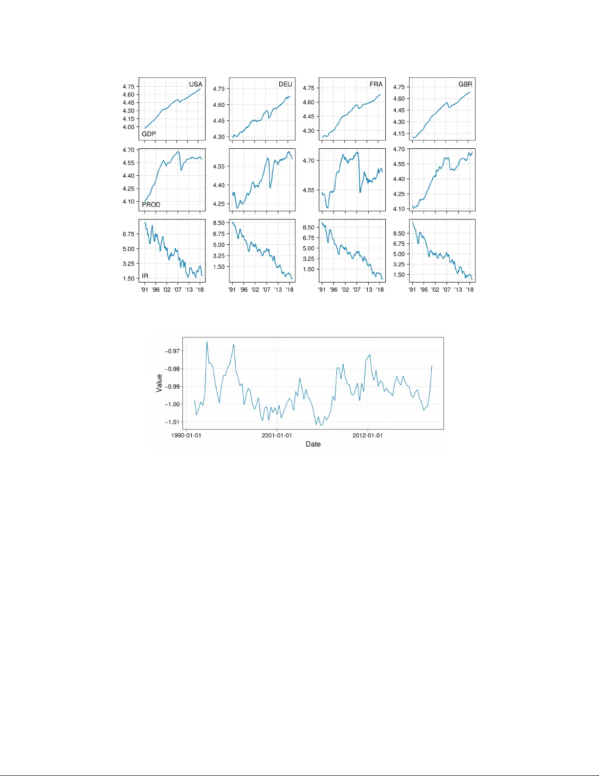
Detecting Coin tegrating Relations in Non-stationary Matrix-V alued Time Series Alain Hecq, Iv an Ricardo ∗ , Ines Wilms Maastric ht Univ ersity , Departmen t of Quantitativ e Economics Jan uary 27, 2025 Abstract This pap er prop oses a Matrix Error Correction Mo del to identify coin tegration relations in matrix- v alued time series. W e hereby allow separate cointegrating relations along the rows and columns of the matrix-v alued time series and use information criteria to select the coin tegration ranks. Through Mon te Carlo sim ulations and a macroeconomic application, we demonstrate that our approac h provides a reliable estimation of the num b er of cointegrating relationships. Keywords : Matrix-v alued time series, Coin tegration rank, Error correction mo del, Information criteria ∗ Corresponding author: Iv an Ricardo, Maastrich t Universit y , Sc ho ol of Business and Economics, Department of Quan titative Economics, P .O.Box 616, 6200 MD Maastrich t, The Netherlands. E-mail: iu.ricardo@maastric htuniv ersity .nl. 1 1 In tro duction Understanding the long-run relationships b et w een key macro economic v ariables is a central fo cus for many economists. Recently , how ever, interest has turned to coin tegration analysis for matrix-v alued time series ( Li and Xiao , 2024 ). Mo deling matrix-v alued time series directly allows researchers to capture long-run relationships across m ultiple dimensions– suc h as b etw een coun tries (ro w dimension) and economic indicators (column dimension) –providing a more comprehensiv e understanding of ho w different economies in teract, co-mo v e, and adjust o v er time. This pap er introduces the Matrix Error Correction Mo del and demonstrates that information criteria can b e reliably used to determine the cointegrating ranks among the different dimensions of the matrix-v alued time series. T o fix ideas, w e first review the standard framework for analyzing multiv ariate cointegrated systems. Let y t , t = 1 , . . . , T , b e an N dimensional time series integrated of order I(1). In the presence of cointegration, the v ector error correction mo del (VECM, see e.g., Johansen and Juselius , 1990 ) ∆y t = d + αβ ′ y t − 1 + p X j =1 Φ j ∆y t − j + e t , (1) captures long-run relationships, where d is the v ector of deterministic terms, 1 and β and α are the N × r coin- tegrating matrix and adjustmen t co efficien ts resp ectiv ely , with r b eing the cointegrating rank. Additionally , Φ j represen ts the j th N × N short-run co efficient matrix, and e t is the N -dimensional error term. When N is small– typically ranging from t w o to five key v ariables –the canonical correlation approac h of Johansen ( 1991 ) can reliably determine the cointegration rank of the matrix Π = αβ ′ . Ho w ever, as N gro ws, this metho d b ecomes less reliable, necessitating alternatives to determine the coin tegrating rank (e.g., Gutierrez , 2003 , Wilms and Croux , 2016 ). T o this end, we exploit the time series’ matrix-v alued structure, where N 1 and N 2 denote the num b er of time series in the ro ws and columns of the observ ed matrix ov er time. F or instance, our empirical analysis examines data from N 1 = 3 economic indicators and N 2 = 4 coun tries o ver T = 116 observ ations, resulting in N 1 N 2 = N = 12 v ariables. This matrix structure allows us to employ a Matrix Error Correction Mo del (MECM), whic h jointly accommo dates the long-run dep endencies across the t w o dimensions of the matrix, similar to the framework recen tly prop osed b y Li and Xiao ( 2024 ). More precisely , we imp ose a Kroneck er structure on the α , β , and Φ j terms of equation ( 1 ) (see Section 2 ). This structure has three b enefits ov er the traditional VECM. First, it enables separate analysis of the cointegration dynamics across the ro ws and columns of the matrix, unlik e the vectorized approac h in equation ( 1 ). W e th us hav e a rank asso ciated with the economic indicators ( r 1 , row rank) and a p otentially differen t rank for the countries ( r 2 , column rank). Second, we allow for a 1 F or simplicity , the deterministic terms are left unrestricted and are not included within the cointegrating vector. 2 partial full-rank cointegrated system where only one of the tw o dimensions of the matrix-v alued time series is rank-restricted. Third, the resulting model is typically far more parsimonious, allo wing for larger data sets than a traditional VECM. While Li and Xiao ( 2024 ) consider the MECM with fixed cointegration ranks mainly from a theoretical p oin t of view, we complement their w ork by pro viding practitioners with practical to ols, in the form of information criteria, to select the cointegration ranks r 1 and r 2 (see Section 3 ). Information criteria hav e b een successfully applied in the cointegration literature ( Aznar and Salv ador , 2002 ; Cheng and Phillips , 2009 ) and can flexibly accommo date matrix-v alued time series. W e demonstrate the go o d p erformance of the information criteria through a Monte Carlo sim ulation study in Section 4 . Finally , our empirical results in Section 5 rev eal a single (restricted) long-run relationship b etw een three economic indicators for the US, German y , F rance, and Great Britain. Replication material for the simulations and empirical analysis are a v ailable at https://github.com/ivanuricardo/MECMrankdetermination . 2 The Matrix Error Correction Mo del Let Y t b e an N 1 × N 2 matrix-v alued time series with I(1) comp onent series that follo ws the MECM( p ) mo del giv en b y ∆Y t = D + U 1 U ′ 3 Y t − 1 U 4 U ′ 2 + p X j =1 Φ 1 ,j ∆Y t − j Φ ′ 2 ,j + E t , (2) where D is the matrix of deterministic terms, U 3 ∈ R N 1 × r 1 and U 4 ∈ R N 2 × r 2 are the coin tegrating ma- trices for the rows and columns of the matrix-v alued time series, U 1 ∈ R N 1 × r 1 and U 2 ∈ R N 2 × r 2 are the corresp onding adjustment co efficients, and Φ 1 ,j ∈ R N 1 × N 1 and Φ 2 ,j ∈ R N 2 × N 2 are the matrix autoregressive co efficien ts ( Li and Xiao , 2024 ). 2 W e assume the errors follow a matrix-v alued normal distribution ( Dawid , 1981 ), namely E t ∼ M V N ( 0 , Σ 1 , Σ 2 ) ⇔ vec( E t ) ∼ N (v ec( 0 ) , Σ 2 ⊗ Σ 1 ) , where Σ 1 ∈ R N 1 × N 1 and Σ 2 ∈ R N 2 × N 2 are p ositive definite matrices capturing the relations b etw een the ro ws and columns of the matrix-v alued errors, M V N ( · , · , · ) denotes the matrix-v alued normal distribution, and N ( · , · ) denotes the m ultiv ariate normal distribution. Reorganizing equation ( 2 ) to the traditional vector- 2 In the case of a stationary matrix AR( p ), different ranks are used for each matrix to distinguish b etw een different right and left null space commonalities in the U i , see Hecq et al. ( 2024 ). 3 v alued set-up, where vec( Y t ) = y t , giv es the restricted VECM ∆y t = d + ( U 2 ⊗ U 1 ) | {z } α ( U 4 ⊗ U 3 ) ′ | {z } β ′ y t − 1 + p X j =1 ( Φ 2 ,j ⊗ Φ 1 ,j ) | {z } Φ j ∆y t − j + e t . The MECM in equation ( 2 ) thus implies a Kroneck er structure on the adjustment co efficients α , the coin- tegrating matrix β , and short-run co efficients Φ j of equation ( 1 ). The imp osed Kroneck er structure puts restrictions on the co efficien ts by s eparating the cointegrating relations and adjustmen t co efficients across the tw o dimensions of the matrix-v alued time series. This sepa- ration not only enhances interpretabilit y but also yields a substantial reduction in the num b er of parameters to be estimated. The total num b er of effectiv e parameters, excluding the constan t term, is giv en b y ψ ( r 1 , r 2 , p ) = r 1 (2 N 1 − r 1 ) + r 2 (2 N 2 − r 2 ) + p ( N 2 1 + N 2 2 ) . (3) As an example, consider a scenario where ( N 1 , N 2 ) = (3 , 4), ( r 1 , r 2 ) = (1 , 1) and p = 2, then the MECM requires estimating 62 parameters, whereas a comparable VECM with N = 12, r = 1, and p = 2 would require estimating 311 parameters. Remark 1. Model ( 2 ) is not uniquely identifiable without additional restrictions on the parameters. T o resolv e this, we imp ose that the top r 1 × r 1 blo c k of U 3 and the top r 2 × r 2 blo c k of U 4 are the iden tit y matrix and set ∥ Σ 1 ∥ F = 1 such that Σ 1 is identified up to a sign change. Iden tification restrictions on the short-run co efficient matrices Φ j are not required, but in case the dimension-sp ecific matrices Φ 1 ,j and Φ 2 ,j are of interest, the same restriction ma y be used, namely , ∥ Φ 1 ,j ∥ F = 1 for j = 1 , . . . , p . Remark 2. W e sp ecify the short-run dynamics in equation ( 2 ) as a matrix autoregression, follo wing Chen et al. ( 2021 ). It is, how ever, possible to replace this with unrestricted autoregressive comp onents. This substitution w ould increase the n umber of lagged autoregressive parameters from N 2 1 + N 2 2 to N 2 1 N 2 2 . Remark 3. While the Kronec ker pro duct structure forms a natural w ay to reduce the dimensionality in MECMs for N 1 × N 2 matrix-v alued data, note that it would b e interesting to introduce a sp ecification test to inv estigate whether the data supp ort the presence of suc h a Kronec k er pro duct structure. T o this end, an interesting av enue for future research w ould b e to extend the sp ecification test of Chen et al. ( 2021 ) for autoregressiv e models with matrix-v alued time series to the MECM model set-up. Remark 4. W e delib erately fo cus on MECMs of mo derate dimension in this pap er. The curren t MECM can, ho w ever, b e extended to high-dimensional settings. Examples of p ossible extensions include applying tec hniques for stationary high-dimensional matrix-v alued time series ( W ang et al. , 2019 ) to the cointegration case (e.g., nonstationary factor mo dels as in Chen et al. , 2025 ), as well as adapting metho ds for vector error 4 correction models (e.g., sparse methods in Liao and Phillips , 2015 ; Wilms and Croux , 2016 or lo w-rank pro cedures in Cubadda and Mazzali , 2023 ) to the high-dimensional MECM set-up. 3 Estimation and Selection of Cointegration Ranks The log-likelihoo d (up to a constant) of the MECM( p ) mo del in equation ( 2 ) for fixed rank r 1 and r 2 is given b y L ( Θ ) = − T N 1 2 log | Σ 1 | − T N 2 2 log | Σ 2 | − 1 2 T X t =1 tr( Σ − 1 1 ( ∆Y t − U 1 U ′ 3 Y t − 1 U 4 U ′ 2 − p X j =1 Φ 1 ,j ∆Y t − j Φ ′ 2 ,j − D ) × Σ − 1 2 ( ∆Y t − U 1 U ′ 3 Y t − 1 U 4 U ′ 2 − p X j =1 Φ 1 ,j ∆Y t − j Φ ′ 2 ,j − D ) ′ ) (4) where Θ collects all parameters. The ob jective function is non-conv ex, but gradien t descent can b e used to solv e problem ( 4 ) in a computationally efficien t wa y (see Appendix A ). In practice, how ever, the ranks r 1 and r 2 are unknown and m ust b e selected. T o this end, w e use standard information criteria, namely , the Ak aik e Information Criterion (AIC, Ak aike , 1974 ) and Bay esian Information Criterion (BIC, Sch warz , 1978 ) AIC( r 1 , r 2 , p ) = − 2 L ( b Θ ) + 2 ψ ( r 1 , r 2 , p ) , BIC( r 1 , r 2 , p ) = − 2 L ( b Θ ) + ln( T ) ψ ( r 1 , r 2 , p ) , where L ( b Θ ) is the v alue of the log-lik eliho o d at the estimated parameters and ψ ( r 1 , r 2 , p ) denotes the effectiv e n um b er of parameters (see eq. 3 ). 4 Sim ulation Study W e conduct a sim ulation study to in vestigate the performance of our rank selection criteria. The data- generating pro cess (DGP) is examined under tw o scenarios. The first is a MECM(0), which omits the short- run dynamics from the model. The second is a MECM(1) with short-run dynamics. Across all settings, we tak e N 1 = 3 and N 2 = 4 in line with our empirical application and generate T + 100 observ ations from the MECM detailed in App endix B , using the first 100 as burn-in and taking T = 100 and T = 250. The rank selection criteria then estimates MECMs across all p ossible combinations of the ranks ( r 1 , r 2 ), and selects the mo del with the low est information criterion v alue. W e explore four settings of a reduced rank in the MECM: (i) fully reduced ( r 1 = r 2 = 1), (ii) partially reduced first dimension ( r 1 = 1 , r 2 = 4), (iii) partially 5 T able 1: MECM(0): Rank selection with AIC or BIC for T = 100 and T = 250 observ ations. T rue Rank Metho d Av erage Ranks Standard Deviation F requency Correct (1,1) AIC (100) (1.02, 1.00) (0.16, 0.00) (0.98, 1.00) BIC (100) (1.02, 1.00) (0.13, 0.00) (0.98, 1.00) AIC (250) (1.01, 1.00) (0.08, 0.00) (0.99, 1.00) BIC (250) (1.01, 1.00) (0.04, 0.00) (0.99, 1.00) (3,1) AIC (100) (3.00, 1.07) (0.00, 0.26) (1.00, 0.93) BIC (100) (3.00, 1.01) (0.00, 0.04) (1.00, 0.99) AIC (250) (3.00, 1.03) (0.00, 0.17) (1.00, 0.97) BIC (250) (3.00, 1.00) (0.00, 0.00) (1.00, 1.00) (1,4) AIC (100) (1.13, 4.00) (0.34, 0.03) (0.87, 1.00) BIC (100) (1.06, 4.00) (0.24, 0.03) (0.94, 1.00) AIC (250) (1.03, 4.00) (0.18, 0.00) (0.97, 1.00) BIC (250) (1.02, 4.00) (0.14, 0.00) (0.98, 1.00) (3,4) AIC (100) (3.00, 4.00) (0.00, 0.00) (1.00, 1.00) BIC (100) (3.00, 4.00) (0.00, 0.00) (1.00, 1.00) AIC (250) (3.00, 4.00) (0.00, 0.00) (1.00, 1.00) BIC (250) (3.00, 4.00) (0.00, 0.00) (1.00, 1.00) reduced second dimension ( r 1 = 3 , r 2 = 1), and (iv) no rank reduction ( r 1 = 3 , r 2 = 4). T o b etter understand the implications of these ranks in the con text of our empirical application with N 1 = 3 economic indicators and N 2 = 4 countries, note that a rank of (1 , 1) indicates one coin tegrating relation among the N = 12 v ariables, suggesting that all indicators mo v e together across different countries. A rank of (1 , 4) reflects four distinct cointegrating relations, where all indicators co-mo v e for each country separately . A rank of (3 , 1) yields three coin tegrating relations, where all countries co-mov e for eac h indicator separately . Finally , with no rank reduction, the model captures a stationary process with no co-mov ements. T able 1 presen ts the results of the simulation study for the MECM(0) DGP . The results for the MECM(1) DGP are similar and given in T able C.1 of App endix C . With a true rank of (1 , 1), all information criteria select the correct rank at a rate ab o v e 95%, with BIC p erforming b est at a rate of ov er 95%. As the num b er of observ ations grows, b oth AIC and BIC select the correct ranks more often. Similar conclusions hold for cases with ranks (3 , 1) and (1 , 4). AIC and BIC select the correct rank at least 85% of the time with T = 100, and it go es up to 100% with T = 250. Under the full rank case, w e alwa ys correctly select the ranks. 6 Figure 1: Time series plots for macro economic economic indicators (ro ws) and countries (columns). Figure 2: The coin tegrated series ( U 4 ⊗ U 3 ) ′ v ec( Y t − 1 ) capturing the long-run dynamics among the 12 v ariables. 5 Application W e consider quarterly macro economic data from 1991Q1 to 2019Q4 ( T = 116) on N 1 = 3 economic indicators across N 2 = 4 countries. This includes the log levels of real gross domestic pro duct (GDP), the log levels of industrial pro duction (PR OD), and the levels of long-term interest rates for the United States (USA), German y (DEU), F rance (FRA), and Great Britain (GBR). The tw elve time series are shown in Figure 1 . All v ariables are found to b e integrated of order I(1) based on Augmented Dic key-F uller tests. W e estimate a MECM(1) for the rank selection criteria and b oth AIC and BIC select (1 , 1) as cointegrating ranks. This implies one restricted coin tegrating relation across all 12 v ariables, which is visualized in Figure 2 without adjustmen t for the short-run dynamics. The corresp onding estimated cointegrating matrices and adjustmen t coefficients are given in T able 2 . 7 Indicators Coun tries b U 1 b U 3 b U 2 b U 4 GDP -0.084 1.000 USA 0.088 1.000 PR OD -0.201 -0.099 DEU 0.774 0.055 IR -7.843 -0.021 FRA 1.103 -1.092 GBR 0.674 -0.196 T able 2: Estimated parameter v alues for indicators and countries. F rom the estimated indicator-sp ecific cointegrating vector b U 3 , we observe that GDP p ositively co-mo v es with industrial production and long-term in terest rates. F or the coun try-sp ecific cointegrating vector b U 4 , the coin tegrating relationship b etw een the USA and F rance is stronger than that b etw een the USA and either German y or Great Britain. Ac knowledgemen ts. W e thank the editor and referee for their constructive comments which substantially impro v ed the quality of the manuscript. The last author w as financially supp orted by the Dutch Research Council (NW O) under grant num b er VI.Vidi.211.032. References Ak aik e, H. (1974), “A new lo ok at the statistical model iden tification,” IEEE T r ansactions on A utomatic Contr ol , 19, 716–723. Aznar, A. and Salv ador, M. (2002), “Selecting the rank of the cointegration space and the form of the in tercept using an information criterion,” Ec onometric The ory , 18, 926–947. Chen, R.; Giannerini, S.; Goracci, G. and T rapani, L. (2025), “Inference in matrix-v alued time series with common stochastic trends and multifactor error structure,” arXiv pr eprint arXiv:2501.01925 . Chen, R.; Xiao, H. and Y ang, D. (2021), “Autoregressive mo dels for matrix-v alued time series,” Journal of Ec onometrics , 222, 539–560. Cheng, X. and Phillips, P . C. B. (2009), “Semiparametric cointegrating rank selection,” The Ec onometrics Journal , 12, S83–S104. Cubadda, G. and Mazzali, M. (2023), “The vector error correction index mo del: representation, estimation and iden tification,” The Ec onometrics Journal , 27, 126–150. Da wid, A. P . (1981), “Some matrix-v ariate distribution theory: Notational considerations and a Bay esian application,” Biometrika , 68, 265–274. 8 Gutierrez, L. (2003), “On the p ow er of panel cointegration tests: a Monte Carlo comparison,” Ec onomics L etters , 80, 105–111. Hecq, A.; Ricardo, I. and Wilms, I. (2024), “Reduced-Rank Matrix Autoregressive Mo dels: A Medium N Approac h,” arXiv pr eprint arXiv:2407.07973 . Johansen, S. (1991), “Estimation and hypothesis testing of cointegration vectors in gaussian vector autore- gressiv e models,” Ec onometric a , 59, 1551–1580. Johansen, S. and Juselius, K. (1990), “Maxim um likelihoo d estimation and inference on cointegration — with applications to the demand for money ,” Oxfor d Bul letin of Ec onomics and Statistics , 52, 169–210. Li, Z. and Xiao, H. (2024), “Cointegrated matrix autoregression mo dels,” arXiv pr eprint arXiv:2409.10860 . Liao, Z. and Phillips, P . C. (2015), “Automated estimation of vector error correction models,” Ec onometric The ory , 31, 581–646. Sc h warz, G. (1978), “Estimating the dimension of a mo del,” The Annals of Statistics , 461–464. W ang, D.; Liu, X. and Chen, R. (2019), “F actor mo dels for matrix-v alued high-dimensional time series,” Journal of Ec onometrics , 208, 231–248. W ang, D.; Zheng, Y. and Li, G. (2024), “High-dimensional lo w-rank tensor autoregressiv e time series mo d- eling,” Journal of Ec onometrics , 238, 105544. Wilms, I. and Croux, C. (2016), “F orecasting using sparse cointegration,” International Journal of F or e c ast- ing , 32, 1256–1267. 9 A Gradien t Ascen t Algorithm W e detail the gradient ascen t algorithm ( W ang et al. , 2024 ) for maximizing the log-likelihoo d given in equation ( 4 ). W e b egin b y initializing the U i for i = 1 , . . . , 4 and Φ 1 ,j , Φ 2 ,j via the pro jection metho d giv en in Chen et al. ( 2021 ). Σ 1 and Σ 2 are initialized to b e the identit y , while D is initialized to the zero matrix. W e then iterate ov er each parameter individually , using the previous parameters as inputs for the next gradien t. W e hereb y denote ∇L x as the partial gradient of parameter x . Algorithm 1 gives the steps. Algorithm 1 Gradient ascent algorithm for MECM Input : Ranks ( r 1 , r 2 ), lag order p , initialization U (0) i for i = 1 , . . . , 4 and Σ (0) i for i = 1 , 2, step size η · , con vergence tolerance ϵ = 0 . 01, maxiter = 500. rep eat s = 1, 2, . . . D ( s ) ← D ( s − 1) + η D ∇L D ( D ( s − 1) ) U ( s ) 1 ← U ( s − 1) 1 + η U 1 ∇L U 1 ( U ( s − 1) 1 ) U ( s ) 3 ← U ( s − 1) 3 + η U 3 ∇L U 3 ( U ( s − 1) 3 ) normalize U ( s ) 3 Σ ( s ) 1 ← Σ ( s − 1) 1 + η Σ 1 ∇L Σ 1 ( Σ ( s − 1) 1 ) normalize Σ ( s ) 1 U ( s ) 2 ← U ( s − 1) 2 + η U 2 ∇L U 2 ( U ( s − 1) 2 ) U ( s ) 4 ← U ( s − 1) 4 + η U 4 ∇L U 4 ( U ( s − 1) 4 ) normalize U ( s ) 4 Σ ( s ) 2 ← Σ ( s − 1) 2 + η Σ 2 ∇L Σ 2 ( Σ ( s − 1) 2 ) for j = 1 , . . . , p do Φ ( s ) 1 ,j ← Φ ( s − 1) 1 ,j + η Φ 1 ,j ∇L Φ 1 ,j ( Φ ( s − 1) 1 ,j ) normalize Φ ( s ) 1 ,j Φ ( s ) 2 ,j ← Φ ( s − 1) 2 ,j + η Φ 2 ,j ∇L Φ 2 ,j ( Φ ( s − 1) 2 ,j ) end for un til L ( Θ ) ( s ) − L ( Θ ) ( s − 1) < ϵ or s = maxiter Return : Σ ( s ) 1 , Σ ( s ) 2 , U ( s ) 1 , U ( s ) 2 , U ( s ) 3 , U ( s ) 4 , Φ ( s ) 1 , Φ ( s ) 2 , D ( s ) B MECM Reparameterization W e reparameterize the MECM in equation ( 2 ) to a stable MAR ( Li and Xiao , 2024 ). The stable MAR reparameterization excluding the constant term is  β ′ Y t ∆ Y t  = A  β ′ Y t − 1 ∆ Y t − 1  +  β ′ E t E t  , where A :=      ( I r 1 γ 2 + β ′ α ) β ′ B α B      . Here, α = ( U 2 ⊗ U 1 ), β = ( U 4 ⊗ U 3 ), and B = ( Φ 2 ⊗ Φ 1 ). The entries of the matrices U 1 , U 2 , U 3 , and U 4 are generated b y sampling from the standard normal distribution and p erforming a QR decomp osition to 10 orthogonalize. If the DGP has short-run dynamics, the same pro cedure is done with the MAR parameters Φ 1 and Φ 2 . Additionally , the error distribution is E t ∼ M V N ( 0 , Σ 1 , Σ 2 ), where Σ 1 and Σ 2 are diagonal with elements generated by fixing a signal-to-noise ratio of 0 . 7. W e use the maximum eigenv alues of A to determine the signal-to-noise ratio and to ensure we generate an I(1) pro cess in our simulation study . C Additional Sim ulation Results The results for the MECM(1) are given in T able C.1 . In the case with ranks (1 , 1) and T = 100, the correct rank is selected in approximately 90% of cases with the AIC, while BIC selects correctly ov er 99% of cases. When the num b er of observ ations is increased, the frequency of correctly selected ranks goes up to 97% for AIC and 98% for BIC. In the case of partially full ranks and full ranks, we see a similar p erformance in the information criteria. Finally , w e inv estigated the case with errors from a multiv ariate normal distribution instead of a matrix-v alued distribution and obtained similar findings. Results are av ailable up on request. T able C.1: MECM(1): Rank selection with AIC or BIC for T = 100 and T = 250 observ ations. T rue Rank Metho d Av erage Rank Std. Rank F req. Correct (1,1) AIC (100) (1.06, 1.03) (0.23, 0.21) (0.94, 0.97) BIC (100) (1.01, 1.00) (0.08, 0.00) (0.99, 1.00) AIC (250) (1.06, 1.02) (0.23, 0.15) (0.94, 0.98) BIC (250) (1.01, 1.00) (0.08, 0.00) (0.99, 1.00) (3,1) AIC (100) (3.00, 1.23) (0.00, 0.59) (1.00, 0.86) BIC (100) (3.00, 1.01) (0.00, 0.08) (1.00, 0.99) AIC (250) (3.00, 1.10) (0.00, 0.40) (1.00, 0.93) BIC (250) (3.00, 1.01) (0.00, 0.03) (1.00, 0.99) (1,4) AIC (100) (1.01, 4.00) (0.05, 0.00) (0.99, 1.00) BIC (100) (1.01, 4.00) (0.03, 0.00) (0.99, 1.00) AIC (250) (1.00, 4.00) (0.00, 0.00) (1.00, 1.00) BIC (250) (1.00, 4.00) (0.00, 0.00) (1.00, 1.00) (3,4) AIC (100) (3.00, 4.00) (0.00, 0.00) (0.99, 1.00) BIC (100) (3.00, 4.00) (0.00, 0.00) (0.99, 1.00) AIC (250) (3.00, 4.00) (0.00, 0.00) (1.00, 1.00) BIC (250) (3.00, 4.00) (0.00, 0.00) (1.00, 1.00) 11