On the Sample Complexity of One Hidden Layer Networks with Equivariance, Locality and Weight Sharing

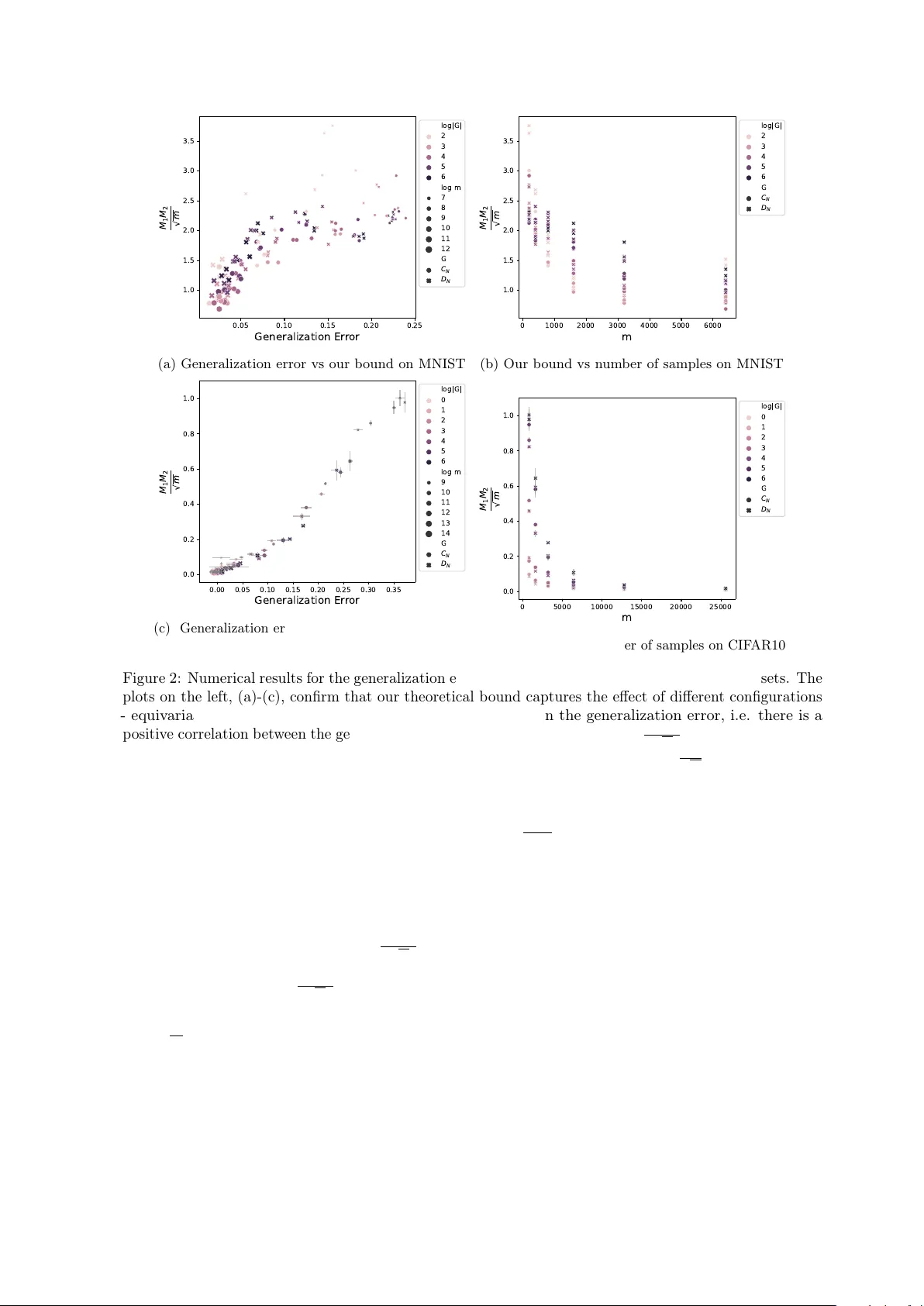
On the Sample Complexit y of One Hidden La y er Net w orks with Equiv ariance, Lo calit y and W eigh t Sharing Arash Beh b o o di Qualcomm AI researc h ∗ Gabriele Cesa Qualcomm AI researc h ∗ Abstract W eight sharing, equiv ariance, and lo cal ﬁlters, as in conv olutional neural netw orks, are b eliev ed to contribute to the sample eﬃciency of neural netw orks. How ever, it is not clear ho w each one of these design c hoices con tributes to the generalization error. Through the lens of statistical learning theory , w e aim to provide insight into this question by characterizing the relativ e impact of each c hoice on the sample complexity . W e obtain low er and upp er sample complexity bounds for a class of single hidden lay er netw orks. F or a large class of activ ation functions, the b ounds dep end merely on the norm of ﬁlters and are dimension-independent. W e also provide b ounds for max-p ooling and an extension to m ulti-lay er net works, b oth with mild dimension dependence. W e pro vide a few tak eaw ays from the theoretical results. It can b e shown that dep ending on the weigh t-sharing mechanism, the non-equiv arian t weigh t-sharing can yield a similar generalization b ound as the equiv ariant one. W e sho w that lo calit y has generalization b eneﬁts, how ev er the uncertaint y principle implies a trade-oﬀ b et ween locality and expressivity . W e conduct extensive exp erimen ts and highlight some consistent trends for these mo dels. 1 In tro duction In recent y ears, equiv ariant neural netw orks hav e gained particular in terest within the machine learning comm unity thanks to their inherent ability to preserve certain transformations in the input data, thereby pro viding a form of inductive bias that aligns with many real-world problems. Indeed, equiv arian t net works hav e shown remark able p erformance in v arious applications, ranging from computer vision to molecular chemistry , where data often exhibit sp eciﬁc forms of symmetry . Equiv arian t net works are closely related to their more traditional counterparts, Conv olutional Neural Netw orks ( CNN s). CNN s are a particular class of neural net works that achiev e equiv ariance to translation. The conv olution op eration in CNN s ensures that the response to a particular feature is the same, regardless of its spatial lo cation in the input data. How ever, equiv ariance extends b ey ond just translation, accommo dating a broader sp ectrum of transformations such as rotations, reﬂections, and scaling. Group Conv olutional Neural Net workss ( GCNN s) [ CW16a ] are the typical example of equiv ariant neural net works. The inductiv e bias in tro duced by equiv ariance, in the form of symmetry preserv ation, oﬀers an in tuitive connection to their generalization capabilities. By enco ding prior knowledge ab out the structure of the data, equiv arian t net works can eﬃciently exploit the inherent symmetries, reducing sample complexity and impro ving generalization p erformance. This ability to generalize from a limited set of examples is crucial to their success. Their mathematical foundation is grounded in group represen tation theory , which provides a p o w erful framework to understand and design neural netw orks that are equiv ariant or inv ariant to the action of a group of transformations. Besides the inductive bias of data symmetry , the generalization b eneﬁts of CNN s and GCNN s are additionally attributed to the weigh t-sharing implemented by the conv olution op eration and the locality implemen ted by the smaller ﬁlter size. In this pap er, we study the impact of equiv ariance, weigh t-sharing, and locality on generalization within the framework of statistical learning theory . Our focus will b e on neural netw orks with one hidden lay er. Similar to works lik e [ VSS22 ]; [ MS23 ], we b elieve that this study provides a ﬁrst step tow ard a b etter understanding of deep er netw orks. Getting dimension-free generalization error bounds constitutes an important line of researc h in the literature. F ollowing this line of work, we provide v arious dimension-free and norm-based b ounds for one hidden la yer netw orks. See App endix J.1 for discussions on the desiderata of learning theory . ∗ Qualcomm AI Research is an initiativ e of Qualcomm T ec hnologies, Inc. 1 ! ! 𝒙 →⋆→ 𝒙(𝑐 ! ) 𝒙(1) ⋰ 𝒘(1, 𝑐 ! ) 𝒘(1,1) ⋰ 𝒘(𝑐 " , 𝑐 ! ) 𝒘(𝑐 " , 1) ⋰ 𝑾 𝑐 " 1 ⋰ ! 1 ! |𝐺| Pool ing ! 𝑐 " 1 ⋰ → 𝑢 → … → ! 𝒚(𝑐 " ) 𝒚(1) ⋰ → σ 𝒚 Input with 𝑐 ! channels output with 𝑐 " channels Group convolution with 𝑐 ! channels: 𝒚 𝑗 = / 𝒘 #$% & ! %'" ⋆ 𝒙(𝑖 ) Wei ght sh arin g with 𝑐 ! channels: 𝒚 𝑗 = / / 𝒘 #$% 𝑘 𝑩 ( ) ('" & ! %'" 𝒙(𝑖) Fina l o utpu t ! ! 𝑩 #$# 𝑩 " ⋰ Fixed mat rice s Locality with !𝑂 * rece ptive fiel d si ze: 𝒚 𝑗 = / 𝒘 #$% + 𝜙 , 𝒙 𝑖 ,-. ) / ! & ! %'" ! ! ! 𝒘 %&'( ) ! 𝒘 %&'( ) 𝜙 #$# 𝒙 𝑖 𝜙 " 𝒙 𝑖 ⋰ ! ! ! ! ! Each patch 𝜙 , 𝒙 𝑖 ! has only 𝑂 * ! element Summary of impacts on the generalization error Group convolution with 𝑐 ! channels: factor 𝒘 #$% #- & " $%-.& ! / Wei ght sh arin g with 𝑐 ! channels: factor max !"# $ % $ 𝒘 &'( ) 𝑘 𝒃 *'! $ *+, &" - ! '("#- " % Locality with !𝑂 * rece ptive fiel d si ze: fac tor 𝑂 * |𝐺| 𝒘 #$% #- & " $%-.& ! / ! 𝒃 "$" ! 𝒃 0)0$" 𝒘 &'( 𝑘 𝑩 * 𝒘 #$% + 𝜙 , 𝒙 𝑖 × → ! 𝜙 + 𝒙 𝑖 → → → Learnable weight Figure 1: Visualization of the net work arc hitectures with equiv ariance, lo cality , and weigh t sharing. On the right, we also summarize how each choice impacts the generalization error in our theory . Con tributions. W e consider a class of one hidden la yer netw orks where the ﬁrst la yer is a multi-c hannel equiv arian t lay er follow ed b y p oin t-wise non-linearity , a p ooling lay er, and the ﬁnal linear lay er. W e assume that the ℓ 2 -norm of the parameters of each lay er is b ounded. F or arc hitectures based on group con volution with p oint-wise non-linearit y , we provide generalization b ounds for v arious p o oling op erations that are en tirely dimension-free. W e obtain a similar norm-based b ound for general equiv ariant netw orks. W e also provide a low er b ound on Rademacher complexity that shows the tigh tness of our b ound. W e extend the results to max-p o oling, com bining v arious cov ering num ber arguments for Rademacher complexit y analysis. The b ound is only dimension-dep enden t on the n umber of hidden lay er c hannels and logarithmic-dep enden t on the group size; otherwise, it is indep enden t of other dimensions. W e also extend the result to m ulti-lay er net works and discuss its limitations. W e show that no gain is observ ed if the analysis is conducted for the netw orks parameterized in the frequency domain. When a lay er replaces the equiv arian t la yer with, not necessarily equiv arian t, w eight-sharing, w e also provide a dimension-free b ound. By studying the b ound, it can be seen that some particular weigh t-sharing schemes, although not all, can pro vide similar generalization guarantees. Next, we give another b ound for netw orks with lo cal ﬁlters and sho w that the lo cality can bring additional gain on top of equiv ariance. W e will then show a trade-oﬀ b et w een locality in the spatial and frequency domains, whic h is imp ortant for band-limited inputs. The uncertain ty principle characterizes the trade-oﬀ. Finally , we pro vide the n umerical v eriﬁcation of our b ounds. The generalization b ounds are all obtained using Rademacher complexity analysis. W e relegate all pro ofs to the appendix. Notations. W e introduce some of the notations used throughout the pap er. W e deﬁne [ n ] := { 1 , . . . , n } for n ∈ N . The term ∥·∥ refers to the ℓ 2 -norm, which for the space of matrices is the F robenius norm. The sp ectral norm of a matrix A is denoted by ∥ A ∥ 2 → 2 . A p ositiv ely homogeneous activ ation function σ ( · · · ) is a function that satisﬁes σ ( λx ) = λσ ( x ) for all λ ≥ 0 . The loss functions are assumed to b e 1 -Lipsc hitz. The matrix of the training data is denoted b y X = [ x 1 . . . x m ] . The terms L ( h ) and ˆ L ( h ) denotes, resp ectiv ely , the test and the training error. 2 Preliminaries Con volution: a simple example. W e start with a simple example of familiar con volutional neural net works, indulging some of the subtleties needed for our later discussions. F or an RGB image input, each con volution ﬁlter will slide o ver the input image and act on its receptiv e ﬁeld b y simple multiplication. If we translate the pixels of the input image, ignoring the c orner pixels, the output of the previous con volution op eration w ould just get translated as w ell. The act of translation is an example of a gr oup 2 action , and the fact that this act shifts the con volution output is an example of equiv ariance prop erty 1 . In what follo ws, we work with a generalized notion of action captured b y group theory , which studies ob jects like translation and rotation that can combine and hav e an inv erse element. W e introduce k ey concepts from group and representation theories necessary to presen t our main results in App endix A . In the rest of this w ork, w e will generally assume a c omp act group G . Note that this includes any ﬁnite group. F or the most part, we will consider A b elian groups, i.e., comm utative groups (suc h as planar rotations or perio dic translations). Equiv ariance. Given tw o spaces X , Y carrying an action of a group G , a function ϕ : X → Y is said to b e equiv ariant with resp ect to G if ϕ ( g .x ) = g .ϕ ( x ) for any x ∈ X , i.e. if ϕ comm utes with the group’s action. F or example, the spaces X , Y could b e vector spaces, and the group action . : G × X → X could b e a linear function. Group Conv olution. If G is a ﬁnite group, the most p opular design choice to construct equiv arian t net works relies on the group conv olution op erator [ CW16a ], thereb y generalizing t ypical con volutional neural net works (CNNs). Sp eciﬁcally , given an input signal x : G → R o ver G and a ﬁlter w : G → R , the group conv olution pro duces another output signal y : G → R deﬁned as: y ( g ) = ( w ⊛ G x )( g ) := X h ∈ G w ( g − 1 h ) x ( h ) . (1) Note that the signals x, w , y can b e represen ted as vectors x , w , y ∈ R | G | ; hence, the con volution op eration can b e expressed as y = W x , where W ∈ R | G |×| G | is a group-circulant matrix encoding G -con volution with the ﬁlter w . Lik e in classical CNNs, one typically considers multi-c hannel input signals x : G → R c 0 , ﬁlters w : G → R c 1 × c 0 and output signals y : G → R c 1 . W e represent a multi-c hannel signal x : G → R c 0 as a stack of features ov er the group G , namely , a tensor ( x (1) , . . . , x ( c 0 )) of shape | G | × c 0 (i.e. with c 0 c hannels and eac h x ( i ) ∈ R | G | ). Then, a con volution lay er consists of c 1 con volutional ﬁlters { w j , j ∈ [ c 1 ] } , eac h of size | G | × c 0 , parametrized by p er-c hannel conv olutions w ( j,i ) ∈ R | G | , i ∈ [ c 0 ] ; the conv olution op eration, whic h yields the output channel j , is giv en by y ( j ) = c 0 X i =1 w ( j,i ) ⊛ G x ( i ) ∈ R | G | , j ∈ [ c 1 ] In summary , a group conv olution lay er can b e visualized as W z }| {      W (1 , 1) W (2 , 1) . . . W ( c 0 , 1) W (1 , 2) W (2 , 2) . . . W ( c 0 , 2) . . . . . . . . . . . . W (1 ,c 1 ) W (2 ,c 1 ) . . . W ( c 0 ,c 1 )      · x z }| {      x (1) ∈ R | G | x (2) ∈ R | G | . . . x ( c 0 ) ∈ R | G |      = y z }| {      y (1) ∈ R | G | y (2) ∈ R | G | . . . y ( c 1 ) ∈ R | G |      (2) Here, any W ( i,j ) ∈ R | G |×| G | blo c k is a group circulan t matrix corresp onding to G , which enco des a G -con volution parameterised b y a ﬁlter w i,j ∈ R | G | . Note that the output of the con volution is a | G | × c 1 signal, i.e. it contains a diﬀerent v alue y ( g , j ) for each group element g ∈ G and output channel j ∈ [ c 1 ] . Note also that the group G naturally acts on a signal x : G → R c as g : x 7→ g .x , with [ g .x ]( h ) = x ( g − 1 h ) . Then, one can show that the group con volution op erator ab ov e is equiv ariant with resp ect to this action on its input and output, i.e., w ⊛ G g .x = g . ( w ⊛ G x ) . A dditionally , it is well known, e.g,. [ CGW18 ]; [ KT18 ], that group conv olutions with learnable ﬁlters in this form parameterize the most general linear equiv arian t maps betw een feature spaces of signals o ver a compact group G . Finally , GCNN t ypically uses an activ ation function applied p oint-wise on the con volution output. In our 1-lay er architecture, a ﬁrst con volution lay er is follow ed by a p oin twise activ ation lay er and, then, a p er-c hannel - av erage or max - p o oling la yer, whic h pro duces c 1 in v ariant features. These ﬁnal features are mixed with the ﬁnal linear lay er u . See Figure 1 for more details. The ﬁnal net work is then given as: h u , w ( x ) := u ⊤ P ◦ σ    P c 0 i =1 w (1 ,i ) ⊛ G x ( i )) . . . P c 0 i =1 w ( c 1 ,i ) ⊛ G x ( i ))    (3) 1 W e would like to emphasize again that the example is not perfect. First, the con volution in CNN is a cross-correlation. Second, the conv en tional CNNs are only approximately translation equiv ariant because of the ﬁnite input size and the corner pixels. 3 where P ( · ) is the p o oling op eration, and w := ( w ( j,i ) ) j ∈ [ c 1 ] ,i ∈ [ c 0 ] is the concatenation of all kernels. 3 Related W orks Equiv ariant and Geometric Deep Learning Previous works attempted to improv e mac hine learning mo dels b y lev eraging prior kno wledge about the symmetries and the geometry of a problem [ Bro+21 ]. A v ariet y of design strategies hav e b een explored in the literature to achiev e group equiv ariance, for example via equiv arian t MLPs [ S ha93 ]; [ Sha89 ]; [ FWW21 ], group conv olution [ CW16a ]; [ KT18 ]; [ Bek+18 ], Lie group conv olution [ Bek20 ]; [ Fin+20 ], steerable conv olution [ CW16b ]; [ CGW18 ]; [ W or+17 ]; [ WHS18 ]; [ W ei+18 ]; [ Tho+18 ]; [ WC19 ]; [ F uc+20 ]; [ Bra+21 ]; [ CL W22 ] and, very recen tly , by using geometric algebra [ RBF23 ]; [ Bre+23 ], to only mention a few. Other previous approaches include [ Mal12 ]; [ DDK16 ]; [ Def+19 ]. Some of these ideas ha ve also been used to generalize conv olution beyond groups to more generic manifolds via the framew ork of Gauge equiv ariance [ Coh+19 ]; [ W ei+21 ]. While equiv ariance is generally considered a p o werful inductive bias that improv es data eﬃciency , this large selection of equiv arian t designs raises the following question: What impact do diﬀerent arc hitectural c hoices hav e on p erformance, and to what exten t do they aid generalization? Generalization Prop erties of Equiv arian t net works Some previous works tried to answ er some asp ects of this question. [ Sha91 ] is one of the ﬁrst works studying the relation b et ween inv ariance and generalization. F or example, [ Sok+17a ] extend the robustness-based generalization b ounds found in [ Sok+17b ] by assuming the set of transformations of interest change the inputs drastically , thereb y pro ving that the generalization error of a G -in v arian t classiﬁer scales 1 / p | G | , where | G | is the cardinality of the ﬁnite equiv ariance group G . [ BM19 ] study the stabilit y of some particular compact group equiv ariant mo dels and also describ e an asso ciated Rademac her complexity and generalization b ound. [ Lyl+20 ] in vestigate the eﬀect of in v ariance under the lenses of the P AC-Ba yesian framework but do not pro vide an explicit b ound. Later, [ EZ21 ] use V C-dimension analysis and deriv e more concrete b ounds. [ Ele22 ] studies compact-group equiv ariance in P AC learning framew ork and equates learning with equiv ariant h yp otheses and learning on a reduced data space of orbit represen tatives to obtain a sample complexity b ound. [ SIK21 ] prop ose a similar idea, pro ving that equiv arian t mo dels w ork in a reduced space, the Quotien t F eature Space ( QFS ), whose volume directly aﬀects the generalization error. While the result relaxes the robustness assumption in [ Sok+17a ], the ﬁnal b ound is sub optimal with resp ect to the sample size. P AC learnability under transformation inv ariance is also studied in [ SMB22 ]. [ ZAH21 ] c haracterize the generalization b eneﬁt of inv arian t mo dels using an argumen t based on the cov ering n umber induced by a set of transformations. More recen tly , [ BCC22 ] leverages a represen tation-theoretic construction of equiv arian t netw orks and provides a norm-based P AC-Ba y esian generalization b ound inspired by [ NBS18 ]. Finally , [ PT23 ] considers a more general setting, allowing for appro ximate, partial, and missp eciﬁed equiv ariance and studying ho w the relation b et ween data and mo del equiv ariance error impacts generalization. Generalization in generic neural netw orks Many works in the literature hav e previously inv estigated the generalization prop erties of deep learning metho ds. [ Zha+17 ] ﬁrst noted that a model trained on random lab els can achiev e small training errors while producing arbitrarily large generalization errors. This result raised a new challenge in the ﬁeld since p opular uniform complexit y measures suc h as V C dimensions are inconsistent with this ﬁnding. This inspired many recen t works whic h tried to explain generalization in terms of other quan tities, such as margin or norms of the learnable weigh ts; a few non-exhaustiv e examples are [ WM19 ]; [ Sok+17b ]; [ NBS18 ]; [ Aro+18 ]; [ BFT17 ]; [ GRS18 ]; [ DR18a ]; [ LS19 ]; [ VSS22 ]; [ Led+21 ]; [ VL20 ]. The P AC Bay esian framework is a particularly p opular metho d. It has b een applied to neural netw orks in man y previous w orks, e.g. see [ NBS18 ]; [ BG22 ]; [ DR17 ]; [ DR18b ]; [ DR18a ]; [ Dzi+20 ]; [ Lot+22 ]. [ Jia+20 ] p erform a thorough exp erimen tal comparison of many complexit y measures and identiﬁes some failure cases; see also [ NK19 ]; [ Koe+21 ]; [ NDR21 ] for further discussion on uniform complexit y measures and their limitations. The norm-based bounds can still be tigh t and informative for shallo w net works considered in this work. Generalization b ounds for Conv olutional neural netw orks As one of the most p opular deep learning architectures, conv olutional neural netw orks (CNNs) hav e received particular attention in the literature. Generalization studies on CNNs are esp ecially relev ant for our wor k since we fo cus signiﬁcantly on equiv ariance to ﬁnite and ab elian groups, which can often b e realiz ed via p erio dic con volution. [ Pit+19 ]; 4 [ LS19 ]; [ VSS22 ]; [ Led+21 ] previously studied these architectures. The authors in [ VSS22 ] represen ted a con volutional la yer as a linear lay er applied on lo cal patches and used Rademac her complexity to get the b ound. In [ LS19 ], the bound is derived using V apnik-Chervonenkis analysis [ VC15 ]; [ GG01 ] and dep ends on the n umber of parameters but indep endent of the n umber of pixels in the input. In [ Gra+22 ], the authors use tw o co vering-n umbers-based b ounds for Rademac her complexity analysis of conv olutional mo dels. Please see Appendix J for further discussions. 4 Sample Complexit y Bounds F or Equiv arian t Net w orks W e consider the group conv olutional netw orks as deﬁned in eq. 3 . W e assume that the input to the net work is b ounded as ∥ x ∥ ≤ b x 2 . Consider the following h yp othesis space: H := { h u , w : ∥ u ∥ ≤ M 1 , ∥ w ∥ ≤ M 2 } , (4) where u ∈ R c 1 , w ∈ R c 0 c 1 | G | . The hypothesis space is the group conv olution netw ork class that has b ounded Euclidean norm on the k ernels. F or this net work, w e derive dimension-free b ounds. Since the p o oling op eration is a p erm utation inv ariant op eration, w e can use Theorem 7 in [ Zah+17 ] to sho w that one can alwa ys ﬁnd t wo functions ϕ : R | G | +1 → R and ρ : R → R | G | +1 suc h that P ◦ z = ϕ  1 | G | P | G | i =1 ρ ( z i )  . W e can provide the following generalization b ound for a subset of such represen tations, namely for p ositiv ely homogeneous ϕ : R → R and ρ : R → R . Theorem 4.1. Consider the hyp othesis sp ac e H deﬁne d in e q. 4 . If P ( · ) is the p o oling op er ation r epr esente d as P ◦ z = ϕ ( 1 | G | 1 ⊤ ρ ( z )) , wher e the two functions ρ ( · ) , ϕ ( · ) and the activation function σ ( · ) ar e al l 1 -Lipschitz p ositively homo gene ous activation function, then with pr ob ability at le ast 1 − δ and for al l h ∈ H , we have: L ( h ) ≤ ˆ L ( h ) + 2 b x M 1 M 2 √ m + 4 r 2 log(4 /δ ) m . The pro of leverages Rademacher complexity analysis and is presented in App endix C.5 . Note that the assumption of positively homogeneity is only needed to utilize the p eeling technique of [ GRS18 ]. W e exp ect that similar techniques from [ VSS22 ] can b e used to extend the result to Lipsc hitz activ ation functions. A verage p o oling. Consider now the sp ecial case of av erage p o oling op eration P ( x ) = 1 | G | 1 ⊤ x . This is a linear lay er; therefore, it can b e combined with the last la yer u to yield a standard t wo-la y er neural net work. W e can utilize the results from [ VSS22 ]; [ GRS18 ]. The combination of the la yer u and av erage p ooling is a linear lay er with the norm M 1 / p | G | , and the matrix W , a circulant matrix, has the F robenius norm p | G | M 2 . The product of these norms w ould b e b ounded by M 1 M 2 . Being a sp ecial case of the mo del in [ VSS22 ], w e can use their results oﬀ-the-shelf to get an upp er b ound on the sample complexity that dep ends only on M 1 M 2 for Lipschitz-activ ation functions (Theorem 2 of [ VSS22 ]). W e provide an indep enden t pro of for p ositiv ely homogeneous activ ation functions in App endix C.2 with a clean form. Note that the authors in [ VSS22 ] pro vide a result for a verage p o oling that con tains the term O ϕ , the maximal num ber of patc hes that any single input co ordinate app ears. In our case, this term equals | G | , whic h is canceled out b y the av erage p ooling term. Their bound dep ends on the spectral norm of the underlying circulant matrix, which can b e bigger than the norm of the ﬁlter pro vided here. But, their pro of can b e rework ed with the norm of conv olutional ﬁlter instead, in which case, their result will be our sp ecial case. Impact of group size. The ab o v e theorem is dimension-free, and there is no dep endence on the n umber of input and output channels c 0 and c 1 , as w ell as the group size | G | . Note that for av erage p ooling and suﬃciently smo oth activ ation functions, w e can use even the stronger result (Theorem 4 of [ VSS22 ]) and get a b ound that dep ends on M 1 M 2 → 2 / p | G | , where M 2 → 2 is the sp ectral norm of W . This manifests the impact of group size on the generalization similar to [ Sok+17a ]; [ BCC22 ]. 2 F or all the results in the pap er, we can use a data-dep enden t bound on the input. Namely , it suﬃces to assume that max i ∈ [ m ] ∥ x i ∥ ≤ b x . 5 Max p ooling. W e cannot rely on the previous results for the max p o oling op eration since the peeling argumen t w ould not w ork. Theorem 7 and 8 of [ VSS22 ] provide a bound for max p o oling, how ev er their net work do es not contain the linear aggregation u after max-po oling, and their b ound contains dimension dep endencies suc h as log ( | G | c 1 ) or log ( m ) . W e pro vide v arious b ounds for max p o oling in App endix C.3 and C.4 . The pro of technique is diﬀeren t from the abov e results. Again, the bounds hav e diﬀerent dimension dep endencies. W e believe these dep endencies are proof artifacts. Removing them w ould b e an in teresting direction for future work. T o summarize, w e hav e established that for a single hidden lay er group con volution net work, w e can ha ve a dimension-free b ound that depends merely on the norm of ﬁlters. R emark 4.2 (F requency Domain Analysis) . The authors in [ BCC22 ] impro ved the P AC-Ba y esian gener- alization b ound by conducting their analysis using the represen tation in the frequency domain. In our Rademac her analysis, suc h a shift would not bring an y additional gain, and we recov er the same b ound. W e provide the details in the supplemen tary materials. 4.1 Bounds for Multi-La yer Equiv ariant Netw ork In this section, we study a simple extension to multi-la yer group equiv arian t netw orks. Consider the follo wing net work with L hidden lay er: h u , { w ( l ) ,l ∈ [ L ] } ( x ) := u ⊤ P ◦ σ ( W ( L ) σ ( W ( L − 1) . . . σ ( W (1) ) x . . . ) (5) where P ( · ) is the av erage p o oling op eration, σ ( · ) is the ReLU function. Eac h linear lay er W l is the same as the mapping in eq. 2 but with c l − 1 and c l as the input and output channels. The new hypothesis space is given by: H ( L ) :=  h u , { w ( l ) ,l ∈ [ L ] } : ∥ u ∥ ≤ M 1 , ∥ w i ∥ ≤ M i +1 , i ∈ [ L ]  . (6) W e hav e the following theorem. Theorem 4.3. Consider the hyp othesis sp ac e H ( L ) deﬁne d in e q. 6 . W ith pr ob ability at le ast 1 − δ and for al l h ∈ H , we have: L ( h ) ≤ ˆ L ( h ) + 2 b x | G | L − 1 2 M 1 M 2 . . . M L +1 √ m + 4 r 2 log(4 /δ ) m . The pro of can b e found in App endix C.6 . W e ﬁrst comment on the dimension dep endency of the b ound. Although our b ound has no dep endence on the num ber of input and hidden la yer channels, it still has dep endence on | G | ( L − 1) / 2 . It is not entirely dimension-free. Using some other techniques, for example, see Section 3 in [ GRS18 ], it can b e improv ed to ( L − 1) log | G | for L > 1 . Ho wev er, dimension dep endence is only one concern of the ab o ve result. It is worth p ointing out that the generalization b ounds for deep er netw orks suﬀer from many shortcomings and generally fail to correlate w ell with the empirical generalization error. F or example, v arious norm b ounds were considered in [ Jia+20 ], and the correlation with the generalization error was explored. Generally , the norm-based b ounds p erformed p o orly , while sharpness-a ware b ounds show ed promises. Besides, in [ NK19 ], the norm-based bounds w ere sho wn to increase drastically with the training set size, leading to looser bounds with increasing training set size. Therefore, we think these norm-based b ounds hav e limitations in deep net work generalization analysis. 4.2 Lo w er b ound on the Rademacher Complexity Analysis A natural question that migh t come up is whether the obtained b ound is tight or not. In this section, we pro vide an answ er to this b y sho wing that the Rademac her complexity is low er b ounded similarly for a class of netw orks. Theorem 4.4. Consider the hyp othesis sp ac e H deﬁne d in e q. 4 . If P ( · ) is the aver age p o oling op er ation, and σ ( · ) is the R eLU activation function, then ther e is a data distribution such that the R ademacher c omplexity is lower b ounde d by c b x M 1 M 2 √ m wher e c is an indep endent c onstant. The pro of is provided in the Appendix E . Note that Rademac her complexity (RC) b ounds are kno wn to b e tigh t for shallow mo dels, such as SVMs. Indeed, if one ﬁxes the ﬁrst lay er and only trains the last linear lay er with weigh t decay , the model is equiv alen t to hard-margin SVM, for whic h RC b ounds are tigh t. W e also pro vide additional evidence in the n umerical result section. 6 5 General Equiv ariant Net w orks The fo cus of our analysis in the ab ov e section has been on group conv olutional netw orks and related arc hitectures. In particular, w e had considered the equiv ariance for ﬁnite Ab elian groups for which the ﬁlters were implemen ted using m ulti-channel con volution op eration. W e now look at the general equiv arian t netw orks w.r.t. a compact group. As we will see, the analysis for these netw orks would b e based on their MLP structure. W e follow the pro cedure describ ed in [ CW16b ]; [ CL W22 ]; [ WHS18 ]. W e assume a general input space where the action of the compact group G on the space is given by a linear map ρ 0 ( g ) for g ∈ G . F or this space, the ﬁlters of the ﬁrst la yer, similarly to GCNs, are parametrized in the frequency domain. The generalization of F ourier analysis to compact groups is done via the notion of irr e ducible r epr esentations (irreps). An irrep, t ypically denoted b y ψ , can be though t as a frequency component of a signal ov er the group. Using to ols from the representation theory , the map ρ 0 ( g ) can b e represented in the frequency domain as the direct sum of irreps Q ⊤ 0  L ψ L m 0 ,ψ i =1 ψ  Q 0 where m 0 ,ψ is the multiplicit y of the irrep ψ . The matrix Q 0 is a unitary matrix representing the generalized F ourier transform given by ˆ x = Q 0 x . See App endix A.1 for detailed deﬁnitions. A similar frequency domain representation can b e obtained for the hidden lay er in terms of irreps, eac h with m ultiplicity m 1 ,ψ . The blo c k diagonal structure of ﬁlters in the multi-c hannel GCNs given in eq. 33 is no w obtained b y a general blo ck-diagonal structure. The equiv arian t neural netw ork is represen ted as h ˆ u , ˆ W := ˆ u ⊤ Q 2 σ   Q 1 M ψ m 1 ,ψ M i =1 m 0 ,ψ X j =1 ˆ W ( ψ , i, j ) ˆ x ( ψ , j )   . Since w e are working with the p oin t-wise non-linearity σ in the sp atial domain , tw o unitary transformations Q 1 and Q 2 are applied as F ourier transforms from the frequency domain to the spatial domain. The last lay er ˆ u should b e chosen to yield a group in v arian t function, whic h means that the vector ˆ u only aggregates the frequencies of the trivial represen tation ψ 0 , and it is zero otherwise. T o use an analogy with group conv olutional netw orks, Q 1 and Q 2 are the F ourier matrices, and ˆ u is a combination of the p ooling, which pro jects into the trivial represen tation of the group, and the last aggregation step. The general equiv arian t netw orks are deﬁned in F ourier space as follows: H ˆ u , ˆ W := n h ˆ u , ˆ W : ∥ ˆ u ∥ ≤ M 1 ,    ˆ W    ≤ M 2 o . Note that the hypothesis space assumes a b ounded norm of the ﬁlters’ parameters in the frequency domain. F or this hypothesis space, we can get a similar dimension-free bound. Theorem 5.1. Consider the hyp othesis sp ac e H ˆ u , ˆ W of e quivariant networks with b ounde d weight norms. If the activation function σ ( · ) is 1-Lipschitz p ositively homo gene ous, then with pr ob ability at le ast 1 − δ for al l h ∈ H ˆ u , ˆ W , we have: L ( h ) ≤ ˆ L ( h ) + 2 b x M 1 M 2 √ m + 4 r 2 log(4 /δ ) m . The proof is presented in App endix D . This result provides another dimension-free b ounds for equiv arian t net works that dep end merely on the norm of the kernels. Note that the netw ork has a standard MLP structure, so the result can b e obtained using techniques used in [ GRS18 ]. Also, note that cons tructing equiv arian t net works in the frequency domain is useful in steerable net works to deal with contin uous rotation groups [ PG21 ]; [ CL W22 ], while the parametrization in the spatial domain is pursued in works lik e [ Bek20 ]; [ Fin+20 ]. 6 Generalization Bounds for W eigh t Sharing In this section, w e try to answer the question whether the gain of our b ound lies in the sp eciﬁc equiv arian t arc hitecture or weigh t sharing. The answ er is subtle. Indeed, an arbitrary t yp e of weigh t sharing will not bring out the generalization gain. How ev er, weigh t-sharing schemes can lead to a similar gain without necessarily b eing equiv arian t. 7 F or a fair comparison with the group con volution netw ork explained abov e, we consider an architecture with the same num ber of eﬀectiv e parameters shared similarly . The weigh t-sharing netw ork is sp eciﬁed as follo ws: h w.s. u , w ( x ) := u ⊤ P ◦ σ      P c 0 c =1  P | G | k =1 w (1 ,c ) ( k ) B k  x ( c ) . . . P c 0 c =1  P | G | k =1 w ( c 1 ,c ) ( k ) B k  x ( c )      , (7) where B k ’s are ﬁxed | G | × | G | matrices inducing the weigh t sharing scheme. These matrices are not trained using data and merely sp ecify how the weigh ts are shared in the net work. F or example, if B k ’s are chosen as the basis for the space of circulant matrices, the setup b oils down to the group conv olution net work. The corresp onding hypothesis space is deﬁned as: H w.s. =  h w.s. u , w ( x ) : ∥ u ∥ ≤ M 1 , ∥ w ∥ B ≤ M w.s. 2  where ∥ w ∥ B := max l ∈ [ | G | ]          | G | X k =1 w ( j,c ) ( k ) b ⊤ k,l   c ∈ [ c 0 ] ,j ∈ [ c 1 ]        F . The following prop osition provides a purely norm-based generalization b ound. Prop osition 6.1. F or the class of functions h in the hypothesis space H w.s. with the av erage p ooling op eration P , σ ( · ) as a 1 -Lipsc hitz positively homogeneous activ ation function, the generalization error is b ounded as: L ( h ) ≤ ˆ L ( h ) + 2 b x M 1 M w.s. 2 √ m + 4 r 2 log(4 /δ ) m . Note that if b k,l ’s are the ro ws of the circulan t matrices, then w e end up with the same result as b efore with M w.s. 2 = M 2 . Interestingly , if the vectors { b k,l : k ∈ [ | G | ] } ’s are orthogonal to eac h other for each l ∈ [ | G | ] , and all of them hav e unit norm, i.e., ∥ b k,l ∥ = 1 , then we also get M w.s. 2 = M 2 . The conclusion is that the weigh t sharing can impact the generalization similarly to the group conv olution, even if the construction do es not arise from the group conv olution. T his does not generally hold, particularly if the ro w vectors of matrices B k are not orthogonal. Note that throughout the paper, w e hav e not assumed an ything regarding the underlying distribution, which can b e without symmetry . On the other hand, the gain of equiv ariance shows itself for distributions with built-in symmetries if w e assume that the underlying task has in v ariance or equiv ariance prop ert y . 7 Generalization Bounds for Lo cal Filters In previous sections, we observed that the impact of equiv ariance on the generalization is v ery similar to that of w eight sharing under an appropriately chosen basis. Another argumen t relates the generalization b eneﬁts of conv olutional neural netw orks to the use of lo cal ﬁlters, where the same ﬁlter is applied to a n umber of patc hes. The patches hav e low er dimensions, and the ﬁlters similarly hav e low er dimensions than the total input dimension. Note that this goes beyond the b eneﬁt of w eight sharing men tioned in the previous section. One example is Theorem 6 in [ VSS22 ]; we follow their setup. In their case, each con volution op eration w ( j,k ) ⊛ G x ( k ) can b e represented as  w ⊤ ( j,k ) ϕ 1 ( x ( k )) . . . w ⊤ ( j,k ) ϕ | G | ( x ( k ))  , where ϕ l ( · ) represents the patch l . Each patch selects a subset of input entries. The patches Φ = { ϕ l , l ∈ [ | G | ] } are assumed to b e lo c al , in the sense that eac h coordinate in x ( k ) appears at most in O Φ n umber of patches with O Φ < | G | . More formally , for any vector x and a set S ⊂ [ | G | ] , deﬁne the v ector x S := ( x i ) i ∈ S , i.e., with entries selected from the index in S . Deﬁne the patch ϕ l : R | G | → R n ′ as ϕ l ( x ) := x S l for a subset S l . The group conv olution netw ork with lo cality is deﬁned as: h Φ u , w ( x ) = u ⊤ P ◦ σ       P c 0 k =1  w ⊤ (1 ,k ) ϕ l ( x ( k ))  l ∈ [ | G | ] . . . P c 0 k =1  w ⊤ ( c 1 ,k ) ϕ l ( x ( k ))  l ∈ [ | G | ]       . 8 By reorganizing the w eights in each ro w corresponding to each patch, the whole net work is presented as u ⊤ P ◦ σ ( W x ) , where we assume that the matrix W conforms to the set of patc hes Φ . The hypothesis space with lo cality is deﬁned as H Φ = { h Φ u , w ( x ) : ∥ u ∥ ≤ M 1 , ∥ w ∥ ≤ M 2 } . F or this class of functions, it can b e shown that there is a generalization b eneﬁt in using lo cal ﬁlters b esides the gain of equiv ariance or prop er weigh t sharing. This conclusion is captured in the follo wing result. Prop osition 7.1. Consider the hypothesis space of functions H Φ constructed by patc hes Φ , the av erage p ooling operation P , 1 -Lipschitz p ositively homogeneous activ ation function σ . Let O Φ b e the maximal n umber of patches that any input en try app ears in. Then, with probabilit y at least 1 − δ and for all h ∈ H Φ , we hav e: L ( h ) ≤ ˆ L ( h ) + 2 s O Φ | G | b x M 1 M 2 √ m + 4 r 2 log(4 /δ ) m . Compared with the result ab o ve, the lo calit y assumption brings an additional improv ement of O Φ | G | . Although the pro of fo cuses on av erage p o oling and group conv olution, the same results can b e obtained for weigh t sharing. W e should only change the ﬁlter parametrization from the matrix B k basis to the v ector b asis b k giv en as  P | G | k =1 w ( j,c ) ( k ) b k  . The architecture considered in [ VSS22 ] is a single-channel version of our result (see more discussions in App endix J ). In that case, the diﬀerence in their bounds is in using the sp ectral norm of W . How ever, their pro of only needs a b ound on the Euclidean norm of weigh ts, which would end in the same result as ours. The analysis so far has fo cused on the lo cal ﬁlters in the spatial domain. Ho w ever, the ﬁlters are also applied p er frequency in the frequency domain and are, therefore, local. This can b e seen from the blo c k diagonal structure of ﬁlters ( L ψ ˆ w ( ψ )) . In this sense, the ﬁlters in the frequency domain are already lo cal. When the ﬁlters are band-limited in the frequency domain, w e hav e an additional notion of lo cality . In practice, this is useful when the input is also band-limited; therefore, not all the frequencies are useful for learning. This in tro duces a fundamental trade-oﬀ for lo cality b eneﬁts arising from the uncertaint y principle [ DS89 ]; [ FS97 ]. A ccording to the uncertain ty principle, the band-limited ﬁlters with B non-zero comp onen ts will hav e at least | G | /B non-zero entries in the spatial domain (see Section I for more details). The trade-oﬀ is captured in the following prop osition. Prop osition 7.2. Consider the hypothesis space of group conv olution netw orks with band-limited ﬁlters. If the ﬁlters hav e B non-zero en tries in the frequency domain, then the generalization error term in Prop osition 7.1 for the smallest spatial ﬁlters is at least of order O ( b x M 1 M 2 / √ mB ) . As it can be seen, the assumption of band-limitedness can p otentially bring the gain of order 1 /B if the ﬁlters are spatially lo cal. T o summarize, there is a gain in using lo cal ﬁlters. How ev er, since band-limited ﬁlters are more eﬃcient for band-limited signals, the uncertaint y principle imp oses a minimum spatial size for band-limited ﬁlters. 8 Numerical Results Let us ﬁrst introduce the tw o family of groups we consider in our exp erimen ts: the cyclic gr oup C n con taining n discrete rotations and the dihe dr al gr oup D n of n discrete rotations and n reﬂections (see Def. A.2 and Def. A.3 for precise deﬁnitions of these groups). In this section, we v alidate our theoretical results on a v ariation of the rotated MNIST and CIF AR10 datasets where we consider a simpler binary classiﬁcation task (determining whether a digit is smaller or larger than 4 in MNIST and whether an image b elongs to the ﬁrst 5 classes of CIF AR10 or not). Rather than working with raw images, w e pre-pro cess the dataset b y linearly pro jecting each image via a ﬁxed randomly initialized G = D 32 -steerable conv olution lay er [ WC19 ] to a single 6400 -dimensional feature vector 3 - interpreted as a c 0 = 100 -channels signal o ver G = D 32 ; see App endix K for more details 3 This is a random linear transformation of the input images in to feature vectors: the reader can think of this as analogous to reshaping an image b efore feeding it into an MLP , but with some care to preserve rotation and reﬂection equiv ariance. Note also that, since the output ( 6400 ) is muc h larger than the num b er of input pixels, this transformation is practically inv ertible and preserves all relev ant input information. 9 0.05 0.10 0.15 0.20 0.25 Generalization Er r or 1.0 1.5 2.0 2.5 3.0 3.5 M 1 M 2 m log|G| 2 3 4 5 6 log m 7 8 9 10 11 12 G C N D N (a) Generalization error vs our b ound on MNIST 0 1000 2000 3000 4000 5000 6000 m 1.0 1.5 2.0 2.5 3.0 3.5 M 1 M 2 m log|G| 2 3 4 5 6 G C N D N (b) Our bound vs num b er of samples on MNIST 0.00 0.05 0.10 0.15 0.20 0.25 0.30 0.35 Generalization Er r or 0.0 0.2 0.4 0.6 0.8 1.0 M 1 M 2 m log|G| 0 1 2 3 4 5 6 log m 9 10 11 12 13 14 G C N D N (c) Generalization error vs our b ound on CIF AR10 0 5000 10000 15000 20000 25000 m 0.0 0.2 0.4 0.6 0.8 1.0 M 1 M 2 m log|G| 0 1 2 3 4 5 6 G C N D N (d) Our b ound vs num b er of samples on CIF AR10 Figure 2: Numerical results for the generalization error on the rotated MNIST and CIF AR 10 datasets. The plots on the left, (a)-(c), conﬁrm that our theoretical b ound captures the eﬀect of diﬀerent conﬁgurations - equiv ariance groups G , training set sizes m and datasets - on the generalization error, i.e. there is a p ositiv e correlation b et ween the generalization error and our theoretical bound M 1 M 2 √ m across all these cases. On the right, (b)-(d), we v erify the bound decreases following a trend similar to 1 √ m and approaching zero for large training set sizes m . and Fig. 5 for a visualization of this linear pro jection. When constructing equiv ariance to a subgroup G < D 32 , this feature v ector is in terpreted as a c 0 = 100 · | D 32 | | G | -c hannels signal o ver G . W e design our equiv arian t netw orks as in Eq. 3 and use c 1 · | G | ≈ 2000 total intermediate channels for all groups G in the MNIST exp eriments and c 1 · | G | ≈ 4000 in the CIF AR10 ones. The dataset is then augmented with random D 32 transformations to mak e it symmetric. Hence, we exp ect that G -equiv arian t mo dels with G closer to D 32 to p erform b est. In these exp erimen ts, we are in terested in how well our theoretical b ound correlates with the observed trends. In particular, w e fo cus on the M 1 M 2 √ m term which is the main comp onen t in our b ounds. In Fig 2 , w e ev aluate the netw orks on diﬀerent v alues of training set size m and on diﬀerent equiv ariance groups G . W e ﬁrst observe that the M 1 M 2 √ m term correlates well with the empirical generalization error on b oth the MNIST dataset in Fig. 2a and the CIF AR10 dataset in Fig. 2c . In particular, larger groups G ac hieve b oth low er generalization error and low er v alue of our norm b ound. W e also note that this term decreases as 1 / √ m in Fig. 2b , which indicates that our b ound b ecomes non-v acuous as m increases, and w e do not suﬀer from deﬁciencies of other norm based bounds [ NK19 ]. Ov erall, these r esults suggest that our b ound c an explain gener alization acr oss diﬀer ent choic es of e quivarianc e gr oup G , as wel l as diﬀer ent tr aining settings . Next, we inv estigate how other equiv arian t design choices aﬀect generalization and verify if our b ound can mo del this eﬀect. Precisely , when parameterizing the ﬁlters ov er the group G in the frequency (i.e. irr eps ) domain (as in Sec 5 ), it is common to only use a smaller subset of all frequencies. A bandlimited sub-set of frequencies can b e interpreted as a form of lo calit y in the frequency domain, in analogy to the lo cal ﬁlters 10 in Sec 7 . In Fig. 3 , w e exp eriments on CIF AR10 with diﬀerent v ariations of our equiv ariant architecture obtained by v arying the maximum frequency used to parameterize ﬁlters. In these experiments, we keep the training dataset size ﬁxed to m = 3200 and w e only consider the largest groups (since a wider range of frequencies in [0 , . . . , N / 2] can b e chosen). In Fig. 3 , we ﬁnd that our b ound c aptur es the eﬀe ct of lo c ality in the fr e quency domain on the gener alization . Figure 3: Our bound vs. the gener- alization error on CIF AR10 (training set size m = 3200 ) when v arying the maxim um frequency used to param- eterize the ﬁlters, which is the lo cal- it y eﬀect in the frequency domain. Eac h dot and its error bars repre- sen t the mean and standard deviation o ver at least 3 runs with the same conﬁguration. As exp ected, ar chi- te ctur es lever aging a lower fr e quency design achieve lower gener alization err or and our b ound can exactly cap- ture this eﬀect. Note that increased frequencies are still b eneﬁcial for the ﬁnal test p erformance: we study the trade-oﬀ b et ween generalization and test p erformance as a function of the mo del frequency in Fig. 4 . 0.05 0.10 0.15 0.20 0.25 0.30 M 1 M 2 m G = C 1 6 G = D 1 6 0.05 0.10 0.15 0.20 Generalization Er r or 0.05 0.10 0.15 0.20 0.25 0.30 M 1 M 2 m G = C 3 2 0.05 0.10 0.15 0.20 Generalization Er r or G = D 3 2 Max F r eq. 0 1 2 3 4 6 8 10 12 14 16 In Fig. 3 , w e observed that higher frequencies typically lead to worse generalization. F or this reason, w e include a ﬁnal study to explore the eﬀect of lo calit y in the frequency domain - i.e., band-limitation - on the ﬁnal test performance of the mo dels and the asso ciated trade-oﬀs b etw een generalization and expressivit y . Fig. 4 compares the generalization error with the ﬁnal test accuracy of some of our mo dels when v arying the maxim um frequency of the ﬁlters and the training set size m . This visualization highligh ts a particular behavior: lo w-frequency models tend to ac hieve low er generalization error b ecause of worse data ﬁtting (low er test accuracy). Con versely , higher frequency mo dels often show higher generalization errors (esp ecially in the low data regime) but ac hieve m uch higher test p erformance. Moreo ver, high-frequency mo dels b eneﬁt the most from increased dataset size m . These prop erties lead to the (multiple) V-shap ed patterns in Fig. 4 : on the sm aller datasets (ligh t dots in Fig. 4 ), while increasing frequencies leads to improv ed test accuracy , it also increases the generalization error. On the other hand, in the larger dataset (dark dots in Fig. 4 ), higher frequencies directly improv e the test p erformance and even show minor impro vemen ts in generalization error. When v arying dataset size, these diﬀerent b eha viors form multiple V-shap ed patterns in Fig. 4 (highligh ted with the dotted lines). 11 Figure 4: T est accuracy vs. Generalization error on CIF AR10 when v arying the max- imum fr e quency used to parameterize the ﬁlters and the training set size m . Each dot is the av erage p erformance ov er at least 3 runs with the same conﬁguration. In Fig. 3 , w e found that higher frequencies correlated with higher generalization error: here, we study the trade-oﬀ betw een generalization and test p erformance. F or each dataset size m , increasing the frequency impro ves the test p erformance until a certain saturation point; b ey ond that, increased frequencies mostly lead to increased generalization error. W e highligh t this eﬀect b y drawing four dotted lines following the trends for v arying frequen- cies with G = C 32 on four diﬀerent dataset sizes m : the diﬀerent slop es of the curves corresp ond to the diﬀerent saturation eﬀects. 8.1 Main Insigh ts from Numerical Results W e would like to summarize some of the main insights from the numerical examples, some of which p ose in teresting theoretical questions. The generalization error seems to b e lo west at the medium group sizes as seen in MNIST or CIF AR exp erimen ts, although the trend is unclear. There s eems to be a group size that leads to the low est generalization error, and if this conjecture is correct is an op en question. The other observ ation is ab out the relation b et w een test accuracy and the generalization error. In general, it can b e seen that the highest test accuracies ha ve lo wer generalization errors in all the plots in Figure 4 . It is interesting to directly explore the impact of the group size on the test error, whic h requires a diﬀeren t mac hinery . 9 Conclusion In this work, w e provided v arious generalization b ounds on equiv arian t net works with a single hidden la yer as w ell as a b ound for m ulti-lay er neural net works. W e hav e used Rademacher complexity analysis to deriv e these b ounds, where the pro ofs were based on either direct analysis of the Rademacher complexit y or cov ering num b er arguments. The b ounds are mostly dimension-free, as they do not dep end on the input and output dimensions. They only dep end on the norm of learnable w eights. The situation changes for multi-la y er scenarios and max-po oling where some dimension dependency appears in the b ound. In ligh t of the results on the limitation of uniform complexit y b ounds for deep er neural netw orks [ NK19 ]; [ Jia+20 ], we b eliev e that the b ound on m ulti-lay er scenario w ould suﬀer from similar limitations. How ev er, the emergence of some dimensions in the bound for max-p ooling seems related to how cov ering num b er argumen t was applied. Whether the dependency can b e remov ed for max-p o oling is an in teresting researc h direction. W e hav e considered equiv arian t mo dels in spatial and frequency domains, mo dels with weigh t sharing, and local ﬁlters. The ﬁrst insight from our analysis is that suitable weigh t-sharing tec hniques should b e able to provide similar guarantees. This is not surprising, as we did not assume any symmetry in the data distribution. Other w orks in the literature hav e highlighted the b eneﬁt of equiv ariance if such symmetries exist - see, for example, [ SIK21 ]; [ Sok+17a ]. Finally , lo cal ﬁlters can p oten tially provide an additional gain, although the story for band-limited ﬁlters is more subtle. W e also pro vide a low er b ound on Rademacher complexity . W e ha ve conducted extensive numerical exp erimen ts and in vestigated the correlation b et ween our generalization error and the true error, as well as the relation b etw een the n umber of samples, group size, and frequency . W e ha ve fo cused on positively homogeneous activ ation functions. W e exp ect that the result can be extended to general Lipschitz activ ations using tec hniques in [ VSS22 ]. How ev er, the current pro of techniques would 12 not work for norm-based nonlinearities used in equiv ariant literature [ W or+17 ]; [ W ei+18 ]; [ WC19 ]. W e encourage readers to consult App endix J for comparison with other works and future directions. References [Aro+18] Sanjeev Arora et al. “ Stronger Generalization Bounds for Deep Nets via a Compression Approac h”. In : International Confer enc e on Machine L e arning . 2018, pp. 254–263. [BCC22] Arash Behbo odi, Gabriele Cesa, and T aco S. Cohen. “ A pac-bay esian generalization bound for equiv arian t net works”. In: A dvanc es in Neur al Information Pr o c essing Systems 35 (2022), pp. 5654–5668. [Bek+18] Erik J. Bekkers et al. “ Roto-translation cov ariant conv olutional netw orks for medical image analysis”. In: International Confer enc e on Me dic al Image Computing and Computer-Assiste d Intervention (MICCAI) . 2018. [Bek20] Erik J Bekkers. “ B-Spline CNNs on Lie groups”. In: International Confer enc e on L e arning R epr esentations . 2020. [BFT17] P eter L Bartlett, Dylan J F oster, and Matus J T elgarsky. “ Spectrally-normalized margin b ounds for neural netw orks”. In: A dvanc es in Neur al Information Pr o c essing Systems 30 . Ed. by I. Guy on et al. Curran Asso ciates, Inc., 2017, pp. 6240–6249. [BG22] F elix Biggs and Benjamin Guedj. “ Non-V acuous Generalisation Bounds for Shallo w Neural Net works”. In: arXiv:2202.01627 [cs, stat] (F eb. 2022). arXiv: 2202.01627. url : http : //arxiv.org/abs/2202.01627 (visited on 03/07/2022). [BM02] P eter L Bartlett and Shahar Mendelson. “ Rademac her and Gaussian Complexities: Risk Bounds and Structural Results”. In: J. Mach. L e arn. R es. 3.No v (2002), pp. 463–482. [BM19] Alb erto Bietti and Julien Mairal. “ Group Inv ariance, Stability to Deformations, and Com- plexit y of Deep Con volutional Representations”. In: J. Mach. L e arn. R es. 20.1 (Jan. 2019), pp. 876–924. [Bra+21] Johannes Brandstetter et al. “ Geometric and physical quan tities improv e e (3) equiv arian t message passing”. In: arXiv pr eprint arXiv:2110.02905 (2021). [Bre+23] Johann Brehmer et al. “ Geometric Algebra T ransformers”. In: arXiv pr eprint (2023). [Bro+21] Mic hael M Bronstein et al. “ Geometric deep learning: Grids, groups, graphs, geo desics, and gauges”. In: arXiv pr eprint arXiv:2104.13478 (2021). [CGW18] T aco S. C ohen, Mario Geiger, and Maurice W eiler. “ A General Theory of Equiv arian t CNNs on Homogeneous Spaces”. In: arXiv pr eprint arXiv:1811.02017 (2018). [CL W22] Gabriele Cesa, Leon Lang, and Maurice W eiler. “ A Program to Build E(N)-Equiv ariant Steerable CNNs”. In: International Confer enc e on L e arning R epr esentations . 2022. url : https://openreview.net/forum?id=WE4qe9xlnQw . [Coh+19] T aco Cohen et al. “ Gauge equiv arian t conv olutional netw orks and the icosahedral CNN”. In: International c onfer enc e on Machine le arning . PMLR. 2019, pp. 1321–1330. [CW16a] T aco S. Cohen and Max W elling. “ Group Equiv arian t Conv olutional Netw orks”. In: [cs, stat] (F eb. 2016). arXiv: 1602.07576. [CW16b] T aco S. Cohen and Max W elling. “ Steerable CNNs”. In: ICLR 2017 . Nov. 2016. [DDK16] Sander Dieleman, Jeﬀrey De F au w, and Kora y Kavuk cuoglu. “ Exploiting Cyclic Symmetry in Con volutional Neural Netw orks”. In: International Confer enc e on Machine L e arning (ICML) . 2016. [Def+19] Mic haël Deﬀerrard et al. “ DeepSphere: a graph-based spherical CNN”. In: International Confer enc e on L e arning R epr esentations . 2019. [DR17] Gin tare Karolina Dziugaite and Daniel M. Roy. “ Computing nonv acuous generalization b ounds for deep (sto c hastic) neural net works with many more parameters than training data”. In: arXiv pr eprint arXiv:1703.11008 (2017). 13 [DR18a] Gin tare Karolina Dziugaite and Daniel Roy. “ En tropy-SGD optimizes the prior of a P AC- Ba yes b ound: Generalization prop erties of En tropy-SGD and data-dep enden t priors”. en. In: International Confer enc e on Machine L e arning . July 2018, pp. 1377–1386. [DR18b] Gin tare Karolina Dziugaite and Daniel M. Roy. “ Data-dep endent P A C-Ba yes priors via diﬀeren tial priv acy”. In: A dvanc es in Neur al Information Pr o c essing Systems . 2018, pp. 8430– 8441. [DS89] Da vid L. Donoho and Philip B. Stark. “ Uncertain ty Principles and Signal Reco very”. en. In: SIAM Journal on Applie d Mathematics 49.3 (June 1989), pp. 906–931. (Visited on 10/16/2023). [Dzi+20] Gin tare Karolina Dziugaite et al. “ In search of robust measures of generalization”. In: A dvanc es in Neur al Information Pr o c essing Systems 33 (2020), pp. 11723–11733. [Ele22] Bryn Elesedy. “ Group symmetry in P A C learning”. en. In: ICLR 2022 W orkshop on Ge omet- ric al and T op olo gic al R epr esentation L e arning . 2022, p. 9. [EZ21] Bryn Elesedy and Sheheryar Zaidi. “ Prov ably strict generalisation b eneﬁt for equiv ariant mo dels”. In: International Confer enc e on Machine L e arning . PMLR, 2021, pp. 2959–2969. [Fin+20] Marc Finzi et al. “ Generalizing conv olutional neural net works for equiv ariance to lie groups on arbitrary contin uous data”. In: International Confer enc e on Machine L e arning . PMLR, 2020, pp. 3165–3176. [FR13] Simon F oucart and Holger Rauhut. A Mathematic al Intr o duction to Compr essive Sensing . Applied and Numerical Harmonic Analysis. New Y ork, NY: Springer New Y ork, 2013. url : http://link.springer.com/10.1007/978- 0- 8176- 4948- 7 (visited on 06/18/2016). [FS97] Gerald B. F olland and Alladi Sitaram. “ The uncertain ty principle: A mathematical survey”. en. In: The Journal of F ourier Analysis and Applic ations 3.3 (May 1997), pp. 207–238. (Visited on 10/16/2023). [F uc+20] F abian F uchs et al. “ SE(3)-T ransformers: 3D Roto-T ranslation Equiv arian t Atten tion Net- w orks”. In: A dvanc es in Neur al Information Pr o c essing Systems . Ed. b y H. Laro c helle et al. V ol. 33. Curran Asso ciates, Inc., 2020, pp. 1970–1981. url : https://proceedings.neurips. cc/paper_files/paper/2020/file/15231a7ce4ba789d13b722cc5c955834- Paper.pdf . [FWW21] Marc Finzi, Max W elling, and Andrew Gordon Wilson. “ A practical metho d for constructing equiv arian t multila yer p erceptrons for arbitrary matrix groups”. In: International c onfer enc e on machine le arning . PMLR. 2021, pp. 3318–3328. [GG01] Ev arist Giné and Armelle Guillou. “ On consistency of k ernel density estimators for randomly censored data: rates holding uniformly o ver adaptiv e interv als”. In: Ann. Inst. Henri Poinc ar e Pr ob ab. Stat. 37.4 (Aug. 2001), pp. 503–522. [Gra+22] Florian Graf et al. “ On measuring excess capacit y in neural net works”. In: A dvanc es in Neur al Information Pr o c essing Systems 35 (2022), pp. 10164–10178. [GRS18] Noah Golowic h, Alexander Rakhlin, and Ohad Shamir. “ Size-Indep enden t Sample Complexity of Neural Netw orks”. en. In: Confer enc e On L e arning The ory . July 2018, pp. 297–299. [Gun+18] Suriy a Gunasek ar et al. “ Implicit bias of gradien t descent on linear conv olutional netw orks”. In: A dvanc es in neur al information pr o c essing systems 31 (2018). [Jia+20] Yiding Jiang et al. “ F antastic Generalization Measures and Where to Find Them”. In: International Confer enc e on L e arning R epr esentations . 2020. [K o e+21] F rederic Koehler et al. “ Uniform Conv ergence of In terp olators: Gaussian Width, Norm Bounds and Benign Overﬁtting”. en. In: A dvanc es in Neur al Information Pr o c essing Systems . May 2021. url : https://openreview.net/forum?id=FyOhThdDBM (visited on 05/19/2022). [KT18] Risi Kondor and Sh ubhendu T riv edi. “ On the generalization of equiv ariance and conv olution in neural netw orks to the action of compact groups”. In: International Confer enc e on Machine L e arning (ICML) . 2018. [La w+22] Hannah Lawrence et al. “ Implicit Bias of Linear Equiv ariant Netw orks”. In: International Confer enc e on Machine L e arning . PMLR. 2022, pp. 12096–12125. [Led+21] An toine Ledent et al. “ Norm-based generalisation b ounds for deep multi-class con volutional neural netw orks”. In: 35th AAAI Confer enc e on Artiﬁcial Intel ligenc e . AAAI Press, 2021, pp. 8279–8287. 14 [Lot+22] Sanae Lotﬁ et al. “ P AC-ba yes compression b ounds so tight that they can explain gener- alization”. In: A dvanc es in Neur al Information Pr o c essing Systems 35 (2022), pp. 31459– 31473. [LS19] Philip M. Long and Hanie Sedghi. “ Size-free generalization b ounds for conv olutional neural net works”. In: arXiv:1905.12600 [cs, math, stat] (May 2019). arXiv: 1905.12600. [L T11] Mic hel Ledoux and Michel T alagrand. Pr ob ability in Banach sp ac es: isop erimetry and pr o- c esses . Classics in mathematics. OCLC: o cn751525992. Berlin ; London: Springer, 2011. [Lyl+20] Clare Lyle et al. “ On the Beneﬁts of Inv ariance in Neural Netw orks”. In: arXiv pr eprint arXiv:2005.00178 (2020). [LZA21] Zhiyuan Li, Yi Zhang, and Sanjeev Arora. “ Wh y Are Conv olutional Nets More Sample- Eﬃcien t than F ully-Connected Nets?” In: International Confer enc e on L e arning R epr esenta- tions . 2021. [Mal12] Stéphane Mallat. “ Group inv ariant scattering”. In: Communic ations on Pur e and Applie d Mathematics 65.10 (2012), pp. 1331–1398. [MR T18] Mehry ar Mohri, Afshin Rostamizadeh, and Ameet T alw alk ar. F oundations of machine le arning . 2nd ed. Adaptiv e Computation and Mac hine Learning series. London, England: MIT Press, Dec. 2018. [MS23] Ro ey Magen and Ohad Shamir. “ Initialization-Dep enden t Sample Complexity of Linear Predictors and Neural Netw orks”. In: Thirty-seventh Confer enc e on Neur al Information Pr o c essing Systems . 2023. [NBS18] Behnam Neyshabur, Srinadh Bho janapalli, and Nathan Srebro. “ A P AC-Ba yesian Approach to Sp ectrally-Normalized Margin Bounds for Neural Netw orks”. In: International Confer enc e on L e arning R epr esentations . 2018. [NDR21] Jeﬀrey Negrea, Gintare Karolina Dziugaite, and Daniel M. Roy. In Defense of Uniform Con- ver genc e: Gener alization via der andomization with an applic ation to interp olating pr e dictors . T ech. rep. arXiv:1912.04265. arXiv, Sept. 2021. url : (visited on 05/19/2022). [NK19] V aishnavh Nagara jan and J. Zico Kolter. “ Uniform conv ergence may b e unable to explain generalization in deep learning”. In: A dvanc es in Neur al Information Pr o c essing Systems 32 . Ed. by H. W allac h et al. Curran Asso ciates, Inc., 2019, pp. 11615–11626. [PG21] A drien Poulenard and Leonidas J. Guibas. “ A fun ctional approach to rotation equiv ariant non-linearities for T ensor Field Net works”. In: 2021 IEEE/CVF Confer enc e on Computer Vision and Pattern R e c o gnition (CVPR) . 2021, pp. 13169–13178. [Pis80] G. Pisier. “ Remarques sur un résultat non publié de B. Maurey”. In: Seminar on F unctional A nalysis (Polyte chnique) 13.5 (1980), pp. 1–12. [Pis89] Gilles Pisier. The V olume of Convex Bo dies and Banach Sp ac e Ge ometry . 1st ed. Cam bridge Univ ersity Press, Oct. 1989. [Pit+19] K onstantinos Pitas et al. “ Some limitations of norm based generalization bounds in deep neural netw orks”. In: arXiv:1905.09677 [cs, stat] (May 2019). arXiv: 1905.09677. [PT23] Mircea P etrache and Shubhendu T rivedi. “ Appro ximation-Generalization T rade-oﬀs under (Appro ximate) G roup Equiv ariance”. In: arXiv pr eprint arXiv:2305.17592 (2023). [RBF23] Da vid Ruhe, Johannes Brandstetter, and Patric k F orré. “ Cliﬀord group equiv arian t neural net works”. In: arXiv pr eprint arXiv:2305.11141 (2023). [SB14] Shai Shalev-Shw artz and Shai Ben-Da vid. Understanding machine le arning: fr om the ory to algorithms . New Y ork, NY, USA: Cam bridge Univ ersity Press, 2014. [SC08] Ingo Steinw art and Andreas Christmann. Supp ort ve ctor machines . 1st ed. Information science and statistics. New Y ork: Springer, 2008. [Ser77] Jean-Pierre Serre. Line ar r epr esentations of ﬁnite gr oups . Springer, 1977. [SFH17] Sara Sab our, Nicholas F rosst, and Geoﬀrey E. Hinton. “ Dynamic routing betw een capsules”. In: A dvanc es in neur al information pr o c essing systems 30 (2017). 15 [Sha89] J. Shaw e-T aylor. “ Building symmetries into feedforward net works”. In: 1989 First IEE International Confer enc e on Artiﬁcial Neur al Networks, (Conf. Publ. No. 313) . Oct. 1989, pp. 158–162. [Sha91] John Shaw e-T aylor. “ Threshold Netw ork Learning in the Presence of Equiv alences”. In: A dvanc es in Neur al Information Pr o c essing Systems . Ed. by J. Moo dy, S. Hanson, and R.P . Lippmann. V ol. 4. Morgan-Kaufmann, 1991. url : https : / / proceedings . neurips . cc / paper_files/paper/1991/file/087408522c31eeb1f982bc0eaf81d35f- Paper.pdf . [Sha93] J Shaw e-T a ylor. “ Symmetries and discriminability in feedforw ard netw ork architectures”. In: IEEE T r ans. Neur al Netw. (1993), pp. 1–25. [SIK21] Akiy oshi Sannai, Masaaki Imaizumi, and Makoto Ka wano. “ Improv ed generalization b ounds of group in v arian t/equiv arian t deep netw orks via quotien t feature spaces”. In: Unc ertainty in A rtiﬁcial Intel ligenc e . PMLR, 2021, pp. 771–780. [SMB22] Han Shao, Omar Montasser, and A vrim Blum. “ A theory of pac learnability under trans- formation inv ariances”. In: A dvanc es in Neur al Information Pr o c essing Systems 35 (2022), pp. 13989–14001. [Sok+17a] Jure Sok olić et al. “ Generalization Error of Inv arian t Classiﬁers”. In: Artiﬁcial Intel ligenc e and Statistics . 2017, pp. 1094–1103. [Sok+17b] Jure Sokolić et al. “ Robust Large Margin Deep Neural Netw orks”. In: IEEE T r ansactions on Signal Pr o c essing 65.16 (Aug. 2017), pp. 4265–4280. [Tho+18] Nathaniel Thomas et al. “ T ensor Field Net works: Rotation- and T ranslation-Equiv ariant Neural Netw orks for 3D P oint Clouds”. In: arXiv pr eprint arXiv:1802.08219 (2018). [V C15] V N V apnik and A Y a Cherv onenkis. “ On the Uniform Conv ergence of Relativ e F requencies of Ev ents to Their Probabilities”. en. In: Me asur es of Complexity: F estschrift for Alexey Chervonenkis . Ed. by Vladimir V o vk, Harris P apadop oulos, and Alexander Gammerman. Cham: Springer International Publishing, 2015, pp. 11–30. [VL20] Guillermo V alle-Pérez and Ard A. Louis. Gener alization b ounds for de ep le arning . [cs, stat]. Dec. 2020. url : http://arxiv.org/abs/2012.04115 (visited on 08/08/2022). [VSS22] Gal V ardi, Ohad Shamir, and Nathan Srebro. “ The Sample Complexity of One-Hidden-Lay er Neural Netw orks”. In: arXiv:2202.06233 [cs, stat] (F eb. 2022). url : http : / / arxiv . org / abs/2202.06233 (visited on 03/06/2022). [W C19] Maurice W eiler and Gabriele Cesa. “ General E (2) -Equiv arian t Steerable CNNs”. In: Confer- enc e on Neur al Information Pr o c essing Systems (NeurIPS) . 2019. [W ei+18] Maurice W eiler et al. “ 3D Steerable CNNs: Learning Rotationally Equiv ariant F eatures in V olumetric Data”. In: Confer enc e on Neur al Information Pr o c essing Systems (NeurIPS) . 2018. [W ei+21] Maurice W eiler et al. “ Co ordinate Indep endent Conv olutional Netw orks–Isometry and Gauge Equiv arian t Conv olutions on Riemannian Manifolds”. In: arXiv pr eprint (2021). [WHS18] Maurice W eiler, F red A. Hamprec ht, and Martin Storath. “ Learning Steerable Filters for Rotation Equiv arian t CNNs”. In: Confer enc e on Computer Vision and Pattern R e c o gnition (CVPR) . 2018. [WM19] Colin W ei and T engyu Ma. “ Impro ved Sample Complexities for Deep Netw orks and Robust Classiﬁcation via an All-Lay er Margin”. In: arXiv:1910.04284 [cs, stat] (Oct. 2019). arXiv: 1910.04284. [W or+17] Daniel E. W orrall et al. “ Harmonic Netw orks: Deep T ranslation and Rotation Equiv ariance”. In: Confer enc e on Computer Vision and Pattern R e c o gnition (CVPR) . 2017. [WW23] Zihao W ang and Lei W u. The or etic al A nalysis of Inductive Biases in De ep Convolutional Networks . arXiv:2305.08404 [cs, stat]. Ma y 2023. url : . [Zah+17] Manzil Zaheer et al. “ Deep Sets”. In: A dvanc es in Neur al Information Pr o c essing Systems 30 (2017). [ZAH21] Sic heng Zhu, Bang An, and F urong Huang. “ Understanding the Generalization Beneﬁt of Mo del In v ariance from a Data Perspective”. In: A dvanc es in Neur al Information Pr o c essing Systems . 2021. 16 [Zha+17] Chiyuan Zhang et al. “ Understanding deep learning requires rethinking generalization”. In: ICLR 2017 . 2017. (Visited on 07/24/2018). [Zha02] T ong Zhang. “ Cov ering num b er b ounds of certain regularized linear function classes”. In: Journal of Machine L e arning R ese ar ch 2.Mar (2002), pp. 527–550. A An Ov erview of Represen tation Theory and Equiv arian t Net- w orks W e provide a brief o verview of some useful concepts from (compact group) Representation Theory in this supplemen tary section. Deﬁnition A.1 (Group) . A gr oup a set G of elements together with a binary operation · : G × G → G satisfying the following three group axioms: • Asso ciativit y: ∀ a, b, c ∈ G a · ( b · c ) = ( a · b ) · c • Iden tity: ∃ e ∈ G : ∀ g ∈ G g · e = e · g = g • In verse: ∀ g ∈ G ∃ g − 1 ∈ G : g · g − 1 = g − 1 · g = e The inv erse elements g − 1 of an element g , and the iden tity element e are unique . Moreo ver, if the binary op eration · is also c ommutative , the group G is called ab elian gr oup . T o simplify the notation, w e commonly write ab instead of a · b . The order of a group G is the c ar dinality of its set and is indicated by | G | . A group G is ﬁnite when | G | ∈ N , i.e. when it has a ﬁnite n umber of elemen ts. A compact group is a group that is also a compact top ological space with con tinuous group operation. Every ﬁnite group is also compact (with a discrete top ology). W e now presen t tw o examples of ﬁnite groups that w e used throughout our exp erimen ts, the cyclic and the dihe dr al gr oups . Deﬁnition A.2 (Cyclic Group) . The cyclic gr oup C N of order N ∈ N is the group of N discrete rotations b y angle s which are integer m ultiples of 2 π N , i.e. { R p 2 π N | p ∈ [0 , 1 , . . . , N − 1] } . The binary op eration com bines tw o rotations to generate the sum of the tw o rotations. This is represented b y integer sum mo dulo N , i.e. R p 2 π N · R q 2 π N = R ( p + q mod N ) 2 π N Deﬁnition A.3 (Dihedral Group) . The dihe dr al gr oup D N of order 2 N ∈ N is the group of N discrete rotations (by angles which are integer multiples of 2 π N ) and N reﬂections (generated b y a reﬂection along an axis follow ed by an y of the N rotations), i.e. { R p 2 π N | p ∈ [0 , 1 , . . . , N − 1] } ∪ { R p 2 π N F | p ∈ [0 , 1 , . . . , N − 1] } where F is a reﬂection along an axis. Note that the group D N has size 2 N and contains the group C N as a subgroup. Another imp ortan t concept is that of gr oup action : Deﬁnition A.4 (Group Action) . The action of a group G on a set X is a map . : G × X → X , ( g , x ) 7→ g .x satisfying the following axioms: • iden tity: ∀ x ∈ X e.x = x • compatibilit y: ∀ a, b ∈ G ∀ x ∈ X a. ( b.x ) = ( ab ) .x F or example, a group can act on functions ov er the group’s elements: giv en a signal x : G → R , the action of g ∈ G on x is deﬁned as [ g .x ]( h ) := x ( g − 1 h ) , i.e., g "translates" the function x . The orbit of x ∈ X through G is the set G.x := { g .x | g ∈ G } . The orbits of the elements in X form a p artition of X . By considering the equiv alence relation ∀ x, y ∈ X x ∼ G y ⇐ ⇒ x ∈ G.y (or, equiv alen tly , y ∈ G.x ), one can deﬁne the quotient space X /G := { G.x | x ∈ X } , i.e. the set of all diﬀerent orbits. 17 Deﬁnition A.5 (Linear Represen tation) . Given a group G and a vector space V , a linear represen tation of G is a homomorphism ρ : G → GL ( V ) asso ciating to each elemen t of g ∈ G an in vertible matrix acting on V , such that: ∀ g , h ∈ G, ρ ( g h ) = ρ ( g ) ρ ( h ) . i.e., the matrix m ultiplication ρ ( g ) ρ ( h ) needs to b e compatible with the group comp osition g h . The most simple representation is the trivial r epr esentation ψ : G → R , g 7→ 1 , mapping all elements to the multiplicativ e identit y 1 ∈ V = R . The common 2 -dimensional rotation matrices are an example of represen tation on V = R 2 of the group SO(2) : ρ ( r θ ) =  cos θ − sin θ sin θ cos θ  with θ ∈ [0 , 2 π ) . In the complex ﬁeld C , circular harmonics are other representations of the rotation group: ψ k ( r θ ) = e − ikθ ∈ V = C 1 where k ∈ Z is the harmonic’s frequency . Similarly , these representations can b e constructed also for the ﬁnite cyclic gr oup C N ∼ = Z / N Z : ψ k ( p ) = e − ikp 2 π N ∈ V = C 1 with p ∈ { 0 , 1 , . . . , N − 1 } . Regular Representation A particularly imp ortant representation is the r e gular r epr esentation ρ reg of a ﬁnite group G . This represen tation acts on the space V = R | G | of v ectors represen ting functions o ver the group G . The regular representation ρ reg ( g ) of an element g ∈ G is a | G | × | G | p ermutation matrix . Each vector x ∈ V = R | G | can b e interpreted as a function ov er the group, x : G → R , with x ( g i ) b eing i -th entries of x . Then, the matrix-v ector m ultiplication ρ reg ( g ) x represen ts the action of g on the function x which generates the "translated" function g .x . These represen tations are of high imp ortance b ecause they describ e the features of group conv olution net works. Direct Sum Given tw o represen tations ρ 1 : G → GL ( R n 1 ) and ρ 2 : G → GL ( R n 2 ) , their dir e ct sum ρ 1 ⊕ ρ 2 : G → GL( R n 1 + n 2 ) is a represen tation obtained b y stacking the tw o representations as follo ws: ( ρ 1 ⊕ ρ 2 )( g ) =  ρ 1 ( g ) 0 0 ρ 2 ( g )  . Note that this representation acts on R n 1 + n 2 whic h con tains the concatenation of the vectors in R n 1 and R n 2 . By combining c copies of the r e gular r epr esentation via the direct sum, one obtains a representation of G acting on the features of a group conv olution netw ork with c c hannels. F ourier T ransform The classical F ourier analysis of p eriodic discrete functions can b e framed as the representation theory of the Z / N Z group. This is summarised b y the following result: the regular represen tation of G = Z / N Z is equiv alen t to the direct sum of all circular harmonics with frequency k ∈ { 0 , . . . , N − 1 } , i.e. there exists a unitary matrix F ∈ C N × N suc h that: ρ reg ( p ) = F ∗ M k ψ k ( p ) ! F for p ∈ { 0 , . . . , N − 1 } = Z / N Z and where ψ k is the circular harmonic of frequency k as deﬁned earlier in this section. The unitary matrix F is what is t ypically referred to as the (unitary) discr ete F ourier T r ansform op erator, while its conjugate transp ose F ∗ is the Inverse F ourier T r ansform one. By indexing the dimensions of the vector space V ∼ = C N on whic h ρ reg acts with the elements p ∈ { 0 , . . . , N − 1 } of G = Z / N Z , the F ourier transform matrix can b e explicitly constructed as F k,p = 1 √ N ψ k ( p ) = 1 √ N e − ikp 2 π N (8) One can verify that the matrix is indeed unitary . 18 In representation theoretic terms, the circular harmonics { ψ k } k are referred to as the irreducible represen tations (or irr eps ) of the group G = Z / N Z . While w e are mostly interested in commutativ e (ab elian) ﬁnite groups in this work, this construction can b e easily extended to square-integrable signals o ver non-ab elian compact groups by using the more general concept of irreducible representations [ BCC22 ]; [ CL W22 ]. See also [ Ser77 ] for rigorous details about represen tation theory . Notation Giv en a signal x : G → C , we typically write x ∈ V = C | G | to refer to the vector containing the v alues of x at each group element. Note that this is the vector space on whic h ρ reg acts. W e also use ˆ x = F x to indicate the vector of F ourier co eﬃcients and ˆ x to indicate the function associating to eac h frequency k (or, equiv alently , irrep ψ k ) the corresp onding F ourier coeﬃcient ˆ x ( ψ k ) ∈ C . Group Con volution Giv en a vector space V asso ciated with a representation ρ : G → GL ( V ) of a group G , the gr oup c onvolution w ⊛ G x ∈ C | G | of tw o elements x , w ∈ V is deﬁned as ∀ g ∈ G ( w ⊛ G x )( g ) := w T ρ ( g ) T x . (9) What we deﬁned is tec hnically a group cross-correlation and so it diﬀers from the usual deﬁnitions of con volution ov er groups. W e still refer to it as group con volution to follo w the common terminology in the Deep Learning literature. One can pro ve that group conv olution is equiv ariant to G , i.e.: w ⊛ G ρ ( g ) x = ρ reg ( g ) ( w ⊛ G x ) If V = C | G | , then x, w : G → C can b e interpreted as signals ov er the group, and group con volution take the more familiar form ( w ⊛ G x )( g ) = X h ∈ G w ( g − 1 h ) x ( h ) (10) Finally , we recall tw o imp ortant prop erties of the F ourier transform: given tw o signals w , x : G → C , the follo wing properties hold c g .x ( ψ ) = ψ ( g ) ˆ x ( ψ ) (11) \ w ⊛ G x ( ψ ) = ˆ w ( ψ ) ˆ x ( ψ ) (12) Eq. 11 guarantees that a transformation by g of x do es not mix the co eﬃcients asso ciated to diﬀerent irreps/frequencies. Eq. 12 is the t ypical c onvolution the or em . Finally , some of these results related to the F ourier transform are generalized by the following theorems. This last prop erty is related to the more general result expressed by Schur’s L emma : Theorem A.6 (Sch ur’s Lemma) . L et G b e a c omp act gr oup (not ne c essarily ab elian) and ψ 1 and ψ 2 two irr eps of G . Then, ther e exists a non-zer o line ar map W such that ψ 1 ( g ) W = W ψ 2 ( g ) for any g ∈ G (i.e. an equiv ariant line ar map) if and only if ψ 1 and ψ 2 ar e e quivalent r epr esentations, i.e. they diﬀer at most by a change of b asis Q : ψ 1 ( g ) = Qψ 2 ( g ) Q − 1 for al l g ∈ G . A second result generalizes the notion of F ourier transform to represen tations b eyond the regular one: Theorem A.7 (Peter-W eyl Theorem) . L et G b e a c omp act gr oup and ρ a unitary r epr esentation of G . Then, ρ de c omp oses into a dir e ct sum of irr e ducible r epr esentations of G , up to a change of b asis, i.e. ρ ( g ) = U   M ψ m ψ M i ψ   U T Each irr ep ψ c an app e ar in the de c omp osition with a multiplicity m ψ ≥ 0 . In particular, in the case of a regular represen tation, the c hange of basis is giv en precisely b y the F ourier transform matrix F . The combination of these t wo results is typically used in steerable CNNs and other equiv arian t designs to c haracterize arbitrary equiv arian t netw orks b y reducing the study to individual irreducible components. See also the next section. 19 A.1 Equiv ariant Net works W e now discuss some p opular equiv arian t neural net work designs. In this w ork, we consider r e al v alued netw orks with 2 la yers, i.e., we limit our discussion to a h yp othesis class of the form H :=  u T σ ( W x )  . In a G -equiv arian t net work, the group G carries an action on the intermediate features of the model; these actions are sp eciﬁed by gr oup r epr esentations , which we introduced in the previous section. W e assume the action of an element g ∈ G on the input and the output of the ﬁrst la yer is given resp ectiv ely b y the matrices ρ 0 ( g ) and ρ 1 ( g ) . The ﬁrst lay er, including the activ ation function, is equiv arian t with resp ect to G if: ∀ g ∈ G, σ ( W ρ 0 ( g ) x ) = ρ 1 ( g ) σ ( W x ) Instead, the last la yer of the net work is in v arian t with resp ect to the action of the group G on the input data via ρ 0 , which means that: ∀ g ∈ G, u T σ ( W x ) = u T ρ 1 ( g ) σ ( W x ) = u T σ ( W ρ 0 ( g ) x ) GCNNs A typical wa y to construct netw orks equiv arian t to a ﬁnite group G is via group conv olution , whic h we in tro duced in the previous section; this is the Gr oup Convolution neur al network (GCNN) design [ CW16a ]. Indeed, if the representation ρ 1 is chosen to be the dir e ct sum of c 1 copies of the r e gular r epr esentation ρ reg of G , i.e. ρ 1 = L c 1 ρ reg and the input ρ 0 = L c 0 ρ reg also consists of c 0 copies of the regular representation, then the linear lay er W can alwa ys b e expressed as c 1 × c 0 group-con volution linear op erators as in eq. 9 : W =      W (1 , 1) W (2 , 1) . . . W ( c 0 , 1) W (1 , 2) W (2 , 2) . . . W ( c 0 , 2) . . . . . . . . . . . . W (1 ,c 1 ) W (2 ,c 1 ) . . . W ( c 0 ,c 1 )      where each W ( i,j ) ∈ R | G |×| G | is a G -circular matrix (i.e. rows are "rotations" of eac h others via ρ reg ) of the form: W ( i,j ) =    w T ( i,j ) ρ reg ( g 1 ) . . . w T ( i,j ) ρ reg ( g | G | )    In this case, note that the representation ρ 1 acts via permutation and, therefore, an y activ ation function σ whic h is applied to each en try of W x en try-wise is equiv ariant: this includes the typical activ ations used in deep learning (e.g. ReLU). General linear la yer The represen tation theoretic to ols we introduced earlier allow for a quite general framew ork to describe a wide family of equiv arian t netw orks b ey ond group-conv olution by considering the generalization of the F ourier transform w e discussed in the previous section. By using Theorem A.7 , a representation ρ l (for l = 0 , 1 ) decomposes in to direct sum of irreps as follo ws: ρ l = U l   M ψ m l,ψ M i =1 ψ   U ⊤ l , where U l is an orthogonal matrix, and m l,ψ is the multiplicit y of the irrep ψ in the representation ρ l . If dim ψ is the dimensionality of the irrep ψ , the width of the net work n is equal to P m 1 ,ψ dim ψ , and the input dimension d is giv en b y P m 0 ,ψ dim ψ . Next, by com bining this result with Theorem A.6 , an equiv arian t netw ork can b e parameterized en tirely in terms of irreps, which is analogous to a F ourier space parameterization of a conv olutional net work. Deﬁning c W l = U − 1 l W l U l − 1 , the equiv ariance condition writes as ∀ g ∈ G, c W l   M ψ m l − 1 ,ψ M i =1 ψ ( g )   =   M ψ m l,ψ M i =1 ψ ( g )   c W l . 20 A ctiv ation function Deﬁnition Norm ReLU [ WHS18 ]; [ W or+17 ] η ( ∥ x ∥ ) = ReLU( ∥ x ∥ − b ) ( b < = 0) Squashing [ SFH17 ] η ( ∥ x ∥ ) = ∥ x ∥ 2 ∥ x ∥ 2 +1 Gated [ WHS18 ] η ( ∥ x ∥ ) = 1 1+ e − s ( x ) ∥ x ∥ T able 1: Equiv arian t activ ation functions This induces a blo c k structure in ˆ W l , where the ( ψ , i ; ψ ′ , j ) -th blo c k blo c k maps the i -th input blo c k transforming according to ψ to the j -th output blo ck transforming under ψ ′ , with i ∈ [ m l − 1 ,ψ ] and j ∈ [ m l,ψ ′ ] . By Theorem A.6 , there are no linear maps equiv ariant to ψ and ψ ′ whenev er these represen tations are in-equiv alen t; this implies the matrix ˆ W l is sparse since its ( ψ , i ; ψ ′ , j ) -th block is non-zero only when ψ ∼ = ψ ′ . Then, the non-zer o ( ψ , i, j ) -th blo c k (here, we drop the redundan t ψ ′ index) is denoted by ˆ w i,j ( ψ ) and should comm ute with ψ ( g ) for any g ∈ G . This is achiev ed by expressing this matrix as a linear com bination of a few ﬁxed basis matrices spanning the space; see [ BCC22 ]; [ CL W22 ] for more details. In the special case of GCNN with abelian group G , each irrep in the intermediate features o ccurs exactly c 1 times. Similarly , if the input represen tation ρ 0 consists of c 0 copies of the regular representation, each irrep app ears exactly c 0 times in ρ 0 . Then, ˆ w i,j ( ψ ) is the F ourier transform of the ﬁlter w ( i,j ) ∈ R | G | at the frequency/irrep ψ . A ctiv ation function σ Eac h mo dule in an equiv arian t netw ork should commute with the action of the group on its own input in order to guarantee the ov erall equiv ariance of the mo del. Hence, the activ ation function σ used in the intermediate lay er should b e equiv arian t with resp ect to ρ 1 ( g ) as well, i.e., σ ( ρ 1 ( g ) x ) = ρ 2 ( g ) σ ( x ) , ∀ g ∈ G . Diﬀerent activ ation functions are used in the literature. As we use unitary representations, one can use norm nonlinearities, σ ( x ) = η ( ∥ x ∥ ) x ∥ x ∥ for a suitable function η : R + 0 → R + 0 . It can b e seen that σ ( ρ 1 ( g ) x ) = ρ 1 ( g ) σ ( x ) . Some examples are norm ReLU [ W or+17 ], squashing [ SFH17 ] and gated nonlinearities [ WHS18 ]. As introduced in the GCNN paragraph, when the intermediate representation is built from the regular represen tation, an y p oin t wise activ ation is admissible: since the group’s action p erm utes the features’ en tries in the spatial domain, it intert wines with the non-linearit y applied entry-wise. There exist also other type of activ ations, suc h as tensor-pro duct non-linearities (based on the Clebsh-Gordan transform) but we do not consider them here. Last la y er u The last la yer maps the features after the activ ation to a single scalar and is assumed to b e inv arian t. This linear lay er can b e thought of as a sp ecial case of the general framework ab o v e, with the choice of output representation ρ 2 b eing a collection of trivial r epr esentations , i.e., ρ 2 ( g ) = I is the iden tity . Since the trivial representation is an irrep, b y Theorem A.6 , this linear map only captures the in v ariant information in the output of the activ ation function. In the case of a GCNN with point wise activ ation σ , this la yer acts as an av eraging p o oling op erator ov er the | G | en tries of each c hannel and learns the weigh ts to linearly combine the c 1 indep enden t c hannels. Note that one can also include a custom p o oling op erator P ( · ) (e.g., max-p o oling) b et ween the activ ation lay er σ and the ﬁnal la yer u lik e in eq. 3 : this giv es additional freedom to construct the ﬁnal inv ariant features b ey ond just av erage p ooling. B Mathematical Preliminaries This section gathers the main to ols we will use throughout the pro ofs. First, we introduce the decoupling technique [ FR13 ], which will be used in the pro of of the next lemma. Theorem B.1. L et ϵ = ( ϵ 1 , . . . , ϵ m ) b e a se quenc e of indep endent r andom variables with E ϵ i = 0 for al l i ∈ [ m ] . L et x j,k , j, k ∈ [ m ] b e a double se quenc e of elements in a ﬁnite-dimensional ve ctor sp ac e V . If F : V → R is a c onvex function, then: E F    m X j,k =1 j  = k ϵ j ϵ k x j,k    ≤ E F   4 m X j,k =1 ϵ j ϵ ′ k x j,k   , (13) 21 wher e ϵ ′ is an indep endent c opy of ϵ . The following lemma can b e found in [ FR13 ], namely inequality (8.22), within the proof of Prop osition 8.13. W e re-state the lemma and the proof here, as it is of indep enden t interest. Lemma B.2. F or any p ositive semideﬁnite matrix B , for 8 β ∥ B ∥ 2 → 2 < 1 , and R ademacher ve ctor ϵ , we have E ϵ  exp  β ϵ ⊤ B ϵ  ≤ exp  β T r( B ) 1 − 8 β ∥ B ∥ 2 → 2  . Pr o of. W e start by using Theorem B.1 : E  exp  β ϵ ⊤ B ϵ  = E   exp   β X j =1 B j j + β X j  = k ϵ j ϵ k B j k     ≤ (exp ( β T r( B ))) E   exp   4 β X j,k ϵ j ϵ ′ k B j k     Then using the inequalit y E exp( β P m l =1 a 1 ϵ l ) ≤ E exp( β 2 P m l =1 a 2 1 / 2) , we hav e: E   exp   4 β X j,k ϵ j ϵ ′ k B j k     ≤ E    exp    8 β 2 X k   X j ϵ j B j k   2       Next, we can see that: X k   X j ϵ j B j k   2 = ∥ B ϵ ∥ 2 =    B 1 / 2 B 1 / 2 ϵ    2 ≤    B 1 / 2    2 2 → 2    B 1 / 2 ϵ    2 = ∥ B ∥ 2 → 2 ϵ ⊤ B ϵ . Therefore, for 8 β ∥ B ∥ 2 → 2 < 1 , w e get: E  exp  β ϵ ⊤ B ϵ  ≤ exp ( β T r( B )) E  exp  8 β 2 ∥ B ∥ 2 → 2 ϵ ⊤ B ϵ  ≤ exp ( β T r( B )) E  exp  β ϵ ⊤ B ϵ  8 β ∥ B ∥ 2 → 2 . Rearranging the terms yields the ﬁnal result. B.1 Rademac her Complexit y Bounds The generalization analysis of this pap er is based on the Rademac her analysis. W e summarize the main theorems here. The terms L ( h ) and ˆ L ( h ) denotes, resp ectively , the test and the training error, formally deﬁned as follows: L ( h ) = E x ∼ P x ( ℓ ◦ h ( x )) , ˆ L ( h ) = 1 m m X i =1 ℓ ◦ h ( x i ) . (14) The empirical Rademacher complexit y is deﬁned as: R S ( G ) = E ϵ sup g ∈G 1 m m X i =1 ϵ i g ( x i ) , (15) Theorem B.3 (Theorem 26.5, [ SB14 ]) . L et H b e a family of functions, and let S b e the tr aining se quenc e of m samples dr awn fr om the distribution D m . L et ℓ b e a r e al-value d loss function satisfying | ℓ | ≤ c . Then, for δ ∈ (0 , 1) , with pr ob ability at le ast 1 − δ we have, for al l h ∈ H , L ( h ) ≤ ˆ L ( h ) + 2 R S ( ℓ ◦ H ) + 4 c r 2 log(4 /δ ) m . (16) 22 Using Theorem B.3 , w e can focus on ﬁnding upp er b ounds for the empirical Rademacher complexity of ℓ ◦ H . Below, w e sho w how to remov e the loss function ℓ ( · ) and fo cus on H . A function ϕ : R → R is called a contraction if | ϕ ( x ) − ϕ ( y ) | ≤ | x − y | for all x, y ∈ R , or equiv alen tly if the function is 1 -Lipschitz. The con traction lemma is a standard result in equation 4.20 of [ L T11 ]. W e will use that for the Rademacher complexity analysis. Lemma B.4. L et ϕ i : R → R b e contr actions such that ϕ i (0) = 0 . If G : R → R is a c onvex and incr e asing function, then E G sup t ∈ T m X i =1 ϵ i ϕ i ( t i ) ! ≤ E G sup t ∈ T m X i =1 ϵ i t i ! . (17) Let’s rewrite the Rademac her term, including the loss function explicitly: R S ( ℓ ◦ H ) = E ϵ " sup h ∈H 1 m m X i =1 ϵ i ℓ ◦ h ( x i ) # . W e assume a 1 -Lipsc hitz loss function, for which w e can use the contraction lemma, 4.20 in [ L T11 ], to get: R S ( ℓ ◦ H ) ≤ R S ( H ) . So ﬁnding an upper bound on R S ( H ) is suﬃcien t for the generalization error analysis. B.2 Dudley’s Inequalit y and Cov ering Number Bounds Although, for most of the pro ofs, we try to directly b ound the Rademacher complexity , there is a wa y of b ounding it using the cov ering num ber of the underlying set. The cov ering n umber of a set G is the minim um num b er of balls required to cov er the set G with the centers within the set, the distances deﬁned according to a metric d , and the radius ﬁxed of a giv en size ϵ . It is denoted by N ( G , d 0 , ϵ ) . The cov ering can b e understo o d is a wa y approximating each p oin t in G b y a set of ﬁnite p oints of G with the ﬁdelit y ϵ . The following result can b e found in many references including [ FR13 ]; [ BFT17 ]; [ MR T18 ]. Theorem B.5 (Dudley’s Inequality) . The R ademacher c omplexity c an b e upp er b ounde d using the c overing numb er as fol lows E ϵ sup g ∈G 1 m m X i =1 ϵ i g ( x i ) ≤ inf α> 0   4 α + 4 √ 2 √ m Z B S ; G 2 α p log N ( G , d, u ) d u   (18) wher e d 0 ( s, t ) is metric deﬁne d on G for any s, t ∈ G as fol lows: d ( s, t ) = 1 m m X i =1 ( s ( x i ) − t ( x i )) 2 ! 1 / 2 (19) and B S ; G = sup g ∈G r P m i =1 g ( x i ) 2 m . The idea is to ﬁnd a b ound on the cov ering num b er and then use Dudley’s inequality to bound the Rademac her complexit y . C Pro of of Main Theorems C.1 Rademac her Complexit y Bounds for Group Con v olutional Netw orks Consider the group con volutional netw ork with c 0 input channel, c 1 in termediate c hannels, and a last la yer with p ooling and aggregation. The input space is assumed to b e R | G |× c 0 . Remember that the net work w as given as follows: h u , w ( x ) = u ⊤ P ◦ σ    P c 0 k =1 w (1 ,k ) ⊛ G x ( k ) . . . P c 0 k =1 w ( c 1 ,k ) ⊛ G x ( k )    = u ⊤ P ◦ σ ( W x ) , 23 where P ( · ) is the p o oling op eration. W e denote the ﬁrst conv olution lay er with the circulant matrix W x . T o ﬁnd a b ound on the Rademacher complexity , W e start with the following inequalit y , whic h is shared across the pro ofs of some of the other theorems in the pap er: E ϵ sup u , w 1 m m X i =1 ϵ i u ⊤ P ◦ σ ( W x i ) ! = M 1 m E ϵ sup w      m X i =1 ϵ i P ◦ σ ( W x i )      ! . (20) The ab o ve result follows from the Cauc hy-Sc h wartz inequality and p eels oﬀ the last aggregation la yer. W e contin ue the pro ofs from this step. C.2 Pro of for Positiv ely Homogeneous Activ ation F unctions with A verage P o oling (Theorem C.1 ) Theorem C.1. Consider the hyp othesis sp ac e H deﬁne d in e q. 4 . If P ( · ) is the aver age p o oling op er ation, σ ( · ) is a 1 -Lipschitz p ositively homo gene ous activation function, then with pr ob ability at le ast 1 − δ and for al l h ∈ H , we have: L ( h ) ≤ ˆ L ( h ) + 2 b x M 1 M 2 √ m + 4 r 2 log(4 /δ ) m . Pr o of. F or an input x ∈ R | G |× c 0 , the action of the group G on each c hannel is giv en b y the p erm utation of the entries. Supp ose that the G − p erm utations are given b y Π 1 , . . . , Π | G | . W e hav e: E ϵ sup w      m X i =1 ϵ i P ◦ σ ( W x i )      ! = E ϵ    sup w        m X i =1 ϵ i    1 | G | 1 ⊤ σ  P c 0 k =1 w (1 ,k ) ⊛ G x i ( k )  . . . 1 | G | 1 ⊤ σ  P c 0 k =1 w ( c 1 ,k ) ⊛ G x i ( k )               = E ϵ      sup w          m X i =1 ϵ i | G | X l =1 1 | G |      σ  P c 0 k =1 w ⊤ (1 ,k ) Π l x i ( k )  . . . σ  P c 0 k =1 w ⊤ ( c 1 ,k ) Π l x i ( k )                     ≤ E ϵ      sup w | G | X l =1 1 | G |          m X i =1 ϵ i      σ  P c 0 k =1 w ⊤ (1 ,k ) Π l x i ( k )  . . . σ  P c 0 k =1 w ⊤ ( c 1 ,k ) Π l x i ( k )                     ≤ | G | X l =1 1 | G | E ϵ      sup w          m X i =1 ϵ i      σ  P c 0 k =1 w ⊤ (1 ,k ) Π l x i ( k )  . . . σ  P c 0 k =1 w ⊤ ( c 1 ,k ) Π l x i ( k )                     where we used triangle inequalities for the ﬁrst inequality . The second inequalit y follows from swapping the suprem um and the sum. Consider an arbitrary summand for a giv en l . W e ﬁrst use the moment inequalit y to get: E ϵ      sup w          m X i =1 ϵ i      σ  P c 0 k =1 w ⊤ (1 ,k ) Π l x i ( k )  . . . σ  P c 0 k =1 w ⊤ ( c 1 ,k ) Π l x i ( k )                     ≤ v u u u u u u t E ϵ      sup w          m X i =1 ϵ i      σ  P c 0 k =1 w ⊤ (1 ,k ) Π l x i ( k )  . . . σ  P c 0 k =1 w ⊤ ( c 1 ,k ) Π l x i ( k )                2      . (21) 24 W e can contin ue the deriv ation as follows. First, deﬁne w ( j, :) := ( w j,i ) i ∈ [ c 0 ] , which is the w eights used for generating the channel j . Now, using the assumption of p ositiv ely homogeneity , w e hav e: E ϵ      sup w          m X i =1 ϵ i      σ  P c 0 k =1 w ⊤ (1 ,k ) Π l x i ( k )  . . . σ  P c 0 k =1 w ⊤ ( c 1 ,k ) Π l x i ( k )                2      = E ϵ   sup w c 1 X j =1 m X i =1 ϵ i σ c 0 X k =1 w ⊤ ( j,k ) Π l x i ( k ) !! 2   = E ϵ   sup w c 1 X j =1   w ( j, :)   2 m X i =1 ϵ i σ 1   w ( j, :)   c 0 X k =1 w ⊤ ( j,k ) Π l x i ( k ) !! 2   , Since ∥ w ∥ 2 ≤ M 2 2 , we hav e c 1 X j =1   w ( j, :)   2 ≤ M 2 2 . W e use a similar trick to the pap er [ GRS18 ] to fo cus only on one channel for the rest: E ϵ   sup w c 1 X j =1   w ( j, :)   2 m X i =1 ϵ i σ 1   w ( j, :)   c 0 X k =1 w ⊤ ( j,k ) Π l x i ( k ) !! 2   ≤ M 2 2 E ϵ   sup w sup j ∈ [ c l ] m X i =1 ϵ i σ 1   w ( j, :)   c 0 X k =1 w ⊤ ( j,k ) Π l x i ( k ) !! 2   ≤ M 2 2 E ϵ   sup ˜ w : ∥ ˜ w ∥≤ 1 m X i =1 ϵ i σ c 0 X k =1 ˜ w ⊤ ( k ) Π l x i ( k ) !! 2   . No w, w e can use the contraction lemma and get: E ϵ   sup ˜ w : ∥ ˜ w ∥≤ 1 m X i =1 ϵ i σ c 0 X k =1 ˜ w ⊤ ( k ) Π l x i ( k ) !! 2   ≤ E ϵ   sup ˜ w : ∥ ˜ w ∥≤ 1 m X i =1 ϵ i c 0 X k =1 ˜ w ⊤ ( k ) Π l x i ( k ) ! 2   ≤ E ϵ   sup ˜ w : ∥ ˜ w ∥≤ 1 c 0 X k =1 ˜ w ⊤ ( k ) m X i =1 ϵ i Π l x i ( k ) !! 2   ≤ E ϵ        m X i =1 ϵ i Π l x i      2   ≤ mb 2 x , (22) where we used the fact that the permutation matrix Π l is unitary . Putting all this together, we get: | G | X l =1 1 | G | E ϵ      sup w          m X i =1 ϵ i      σ  P c 0 k =1 w ⊤ (1 ,k ) Π l x i ( k )  . . . σ  P c 0 k =1 w ⊤ ( c 1 ,k ) Π l x i ( k )                     ≤ | G | X l =1 1 | G | b x M 1 M 2 √ m = b x M 1 M 2 √ m , whic h ﬁnalizes the desired results. C.3 Max p o oling Op eration - Co v ering Number Based Results Single Channel Output. Before going into another result for max p o oling, we fo cus on a simpler example. W e assume ReLU activ ation throughout this subsection. First, consider the following netw ork: h w ( x ) = P ◦ σ c 0 X k =1 w (1 ,k ) ⊛ G x ( k ) ! where P ( · ) is the max p o oling op eration. Just lik e abov e, we assume that the norm of the parameters is b ounded b y M 2 while the input norm is b ounded by b X . A sp ecial case of this setup has been considered in [ VSS22 ] in Theorem 7, where c 0 = 1 . W e recap their pro of, providing a more reﬁned ﬁnal b ound. The only diﬀerence is that, in our pro of, we use Dudley’s inequality . 25 Theorem C.2 (Single Channel Max p ooling) . Consider the hyp othesis sp ac e H of single channel gr oup c onvolutional network with P ( · ) as max p o oling, and σ ( · ) as R eLU. With pr ob ability at le ast 1 − δ and for al l h ∈ H , we have: L ( h ) ≤ ˆ L ( h ) + b x M 2 √ m  144 √ 2 q log(2(8 √ m + 2) m | G | + 1) log( m )  + 4 r 2 log(4 /δ ) m . Pr o of. The pro of consists of deriving the cov ering num b er N ( H , d, u ) and then using Dudley’s inequality . W e hav e included the essen tial comp onents of suc h pro ofs in the section on mathematical preliminaries. First, we can rewrite the conv olution as: c 0 X k =1 w (1 ,k ) ⊛ G x ( k ) = c 0 X k =1 w ⊤ (1 ,k ) Π g x ( k ) ! g ∈ G =  w ⊤ 1 x g  g ∈ G , where w 1 is the vectorized form of concatenated conv olution vectors, and x g is the vectorized form of concatenated Π g x ( k ) . Using this notation, we hav e: d ( h w , h v ) = 1 m m X i =1  P ◦ σ  w ⊤ x i,g  g ∈ G − P ◦ σ  v ⊤ x i,g  g ∈ G  2 ! 1 / 2 , and using the Lipsc hitz contin uity of max-po oling and ReLU, w e get:    P ◦ σ  w ⊤ x g  g ∈ G − P ◦ σ  v ⊤ 1 x g  g ∈ G    ≤ max g ∈ G   ( w − v ) ⊤ x g   . This means that it suﬃces to get a cov ering num ber for the linear function ( w ⊤ x i,g ) i ∈ [ m ] ,g ∈ G on the extended dataset. W e use the following lemma from [ Zha02 ], whic h is stronger than a similar result using Maurey’s empirical lemma [ Pis80 ]; [ Pis89 ]. Lemma C.3. If h ( x ) = w ⊤ x with ∥ x ∥ p ≤ b x and ∥ w ∥ q ≤ w for 2 ≤ p ≤ ∞ and 1 /p + 1 /q = 1 , then for al l u > 0 log N ( H , ∥·∥ ∞ , u ) ≤ (36( p − 1) w b x /u ) 2 log(2(4 w b x /u + 2) m + 1) . wher e m is the numb er of samples. This lemma b ounds the ℓ ∞ -norm cov ering n umber, which is an upp er b ound on the co vering num ber N ( H , d, u ) used in Dudley’s inequality . In our case, the eﬀective num b er of samples is m | G | , and therefore the co vering num b er is b ounded as: log N ( H , d, u ) ≤ (36 b x M 2 /u ) 2 log(2(4 b x M 2 /u + 2) m | G | + 1) . W e just need to plug the abov e cov ering num b er in to Dudley’s inequalit y and use standard inequalities: 4 α + 4 √ 2 √ m Z B S ; H 2 α p log N ( H , d, u ) d u ≤ 4 α + 4 √ 2 √ m Z b x .M 2 2 α (36 b x M 2 /u ) p log(2(4 b x M 2 /u + 2) m | G | + 1) . d u ≤ 4 α + 4 √ 2 √ m (36 b x M 2 ) p log(2(4 b x M 2 /α + 2) m | G | + 1) log( b x M 2 / 2 α ) b y cho osing α = b x .M 2 / 2 √ m , we get the following b ound: 2 b x M 2 √ m + 4 √ 2 √ m (36 b x M 2 ) q log(2(8 √ m + 2) m | G | + 1) log( √ m ) , whic h yields the desired result. Note that the b ound is indep endent of the n umber of channels c 0 , but has logarithmic dependence on the group size, as well as other constan t terms. In comparison with [ VSS22 ], w e do not hav e the dep endence on the spectral norm of the circulant matrix, although, as we indicated b efore, their proof w orks w ell the norm of parameters as well. In this sense, our result can be seen as the generalization of [ VSS22 ] to the m ulti-channel input. 26 Multi-Channel Output. Next, we focus on the following setup with m ulti-channel conv olution given b y th e matrix W : h u , w ( x ) = u ⊤ P ◦ σ ( W x ) . W e hav e the following theorems for this case. Theorem C.4 (Multiple Channel Max po oling) . Consider the hyp othesis sp ac e H of multiple channel gr oup c onvolutional network with P ( · ) as max p o oling, and σ ( · ) as R eLU. With pr ob ability at le ast 1 − δ and for al l h ∈ H , we have: L ( h ) ≤ ˆ L ( h ) + b x M 1 M 2 √ c 1 √ m  288 √ 2 q log(2(16 √ m + 2) m | G | + 1) log( m )  + 4 r 2 log(4 /δ ) m . Pr o of. W e would need a co vering n umber for h u , w ( X ) := ( h u , w ( x 1 ) , . . . , h u , w ( x m )) in ℓ 2 -norm. W e do this in tw o steps similar to the strategy in [ BFT17 ]. As the ﬁrst step, we ﬁnd a δ 1 -co vering u k for the follo wing set: H 1 = { P ◦ σ ( W X ) : ∥ w ∥ ≤ M 2 } where we used the notation W X to denote the concatenation of all points in the training set, namely: W X = ( P ◦ σ ( W x 1 ) , . . . , P ◦ σ ( W x m )) . T o simplify the notation, we assume that that matrix op erations are broadcasted through X as if we ha ve parallel compute ov er x i ’s. The second step consists of ﬁnding a δ 2 -co vering for the set of u ⊤ u k for each u k ’s from the ﬁrst cov ering. Using these tw o cov erings, W e ha ve: d ( h u , w ( X ) , v l ) ≤ d  h u , w ( X ) , u ⊤ u k  + d  u ⊤ u k , v l  ≤ M 2 d ( P ◦ σ ( W X ) , u k ) + d  u ⊤ u k , v l  ≤ M δ 1 + δ 2 (23) where the norm d is deﬁned in eq. 19 for an y functions deﬁned ov er the dataset ( x 1 , . . . , x m ) . Besides, w e assumed the p oin ts v l and u k are chosen from the cov er to satisfy the norm inequalities ab ov e. The ﬁnal cov ering num b er is the pro duct of the co vering num b ers from each step with the cov ering radius M δ 1 + δ 2 . W e start with the second step, namely to cov er the following set for any u k in the ﬁrst co ver: H 2 ,k := { u ⊤ u k : ∥ u ∥ ≤ M 1 } . The elements of the ﬁrst cov er, u k , are themselves instances of the ﬁrst lay er of the netw ork. Therefore, w e can b ound the second cov ering num ber for all k as follows: N ( H 2 ,k , d, δ 2 ) ≤ sup W N ( { u ⊤ P ◦ σ ( W X ) : ∥ u ∥ ≤ M 2 } , d, δ 2 ) . This is an instance of cov ering linear functions. W e will use the following result from [ Zha02 ], which lev erages Maurey’s empirical lemma. Lemma C.5. If h ( x ) = w ⊤ x with ∥ x ∥ p ≤ b x and ∥ w ∥ q ≤ w , then log N ( H , d, u ) ≤ (2 wb x /u ) 2 log(2 m + 1) . wher e m is the numb er of samples. Since the norm of u is bounded by M 1 , we only need to b ound the norm of u k . First, note that ∥ P ◦ σ ( W X ) ∥ 2 = P m i =1 ∥ P ◦ σ ( W x i ) ∥ 2 . F or each element of the sum, we can get the following upp er 27 b ound: ∥ P ◦ σ ( W x i ) ∥ 2 = c 1 X i =1      P ◦ σ c 0 X k =1 w ( i,k ) ⊛ G x ( k ) !      2 ≤ c 1 X i =1      max c 0 X k =1 w ( i,k ) ⊛ G x ( k ) !      2 ≤ c 1 X i =1 c 0 X k =1   max  w ( i,k ) ⊛ G x ( k )    ! 2 ≤ c 1 X i =1 c 0 X k =1   w ( i,k )   ∥ x ( k ) ∥ ! 2 ≤ c 1 X i =1 c 0 X k =1   w ( i,k )   2 ! c 0 X k =1 ∥ x ( k ) ∥ 2 ! ≤ ∥ x ∥ 2 c 1 X i =1 c 0 X k =1   w ( i,k )   2 ≤ b 2 x M 2 1 , where the ﬁrst inequality follo ws from the prop erty of ReLU, and the thrid inequality follo ws from Y oung’s con volutional inequalit y . Using this inequalit y , w e can use Lemma C.5 to get the following: log N ( H 2 ,k , d 0 , δ 2 ) ≤ (2 b x M 1 M 2 √ m/δ 2 ) 2 log(2 m + 1) . (24) No w we can mov e to the cov ering n umber for H 1 = { P ◦ σ ( W X ) : ∥ w ∥ ≤ M 1 } . Given that the ReLU function is 1-Lipschitz, it suﬃces to ﬁnd a cov ering for P ( W X ) , and note that the cov ering norm is a mixed norm, namely: d ( P ( W X ) , U ) = 1 m m X i =1 ∥ P ( W x i ) − U i ∥ 2 ! 1 / 2 =   1 m m X i =1 c 1 X j =1 max c 0 X k =1 w ( j,k ) ⊛ G x i ( k ) ! − U i,j ! 2   1 / 2 . T o ﬁnd the co vering n umber, we use the following set of inequalities: d ( P ( W X ) , U ) ≤   max i ∈ [ m ] c 1 X j =1 max c 0 X k =1 w ( j,k ) ⊛ G x i ( k ) ! − U i,j ! 2   1 / 2 ≤   max i ∈ [ m ] c 1 X j =1   w ( j, :)   2 max c 0 X k =1 w ( j,k )   w ( j, :)   ⊛ G x i ( k ) ! − U i,j   w ( j, :)   ! 2   1 / 2 . Supp ose that we ﬁnd a co ver ˜ U i,j that satisﬁes the follo wing inequality max i ∈ [ m ] ,j ∈ [ c 1 ]      max c 0 X k =1 w ( j,k )   w ( j, :)   ⊛ G x i ( k ) ! − ˜ U i,j      ≤ δ 1 M 1 . (25) Then, it is easy to see that since P c 1 j =1   w ( j, :)   2 ≤ M 1 , then d ( P ( W X ) , U ) =   1 m m X i =1 c 1 X j =1 max c 0 X k =1 w ( j,k ) ⊛ G x i ( k ) ! −   w ( j, :)   ˜ U i,j ! 2   1 / 2 ≤ δ 1 . T o ﬁnd suc h cov ering, ﬁrst ﬁnd a cov er for this set:    max c 0 X k =1 ˜ w ( k ) ⊛ G x i ( k ) !! i ∈ [ m ] : ∥ ˜ w ∥ ≤ 1    . 28 Note that this is a sp ecial case of the cov ering num b er of the single-c hannel netw orks, which w e had computed ab ov e. This set is the super-set of functions represen ted by each c hannel when the weigh ts are normalized to hav e unit norm. W e ﬁnd c 1 indep enden t cov ers, one for each channel, and this will giv e us the desired cov ering in eq. 25 . W e use the co vering num b er for the single c hannel case using M 2 = 1 and u = δ 1 / M 2 (whic h basically do es not change the b ound on the co vering n umber) to get the ultimate co vering n umber for this lay er given by: log N ( H 1 , d, δ 1 ) ≤ c 1 N ( H , d, δ 1 / M 2 ) ≤ c 1 (36 b x M 2 /δ 1 ) 2 log(2(4 b x M 2 /δ 1 + 2) m | G | + 1) . (26) The ﬁnal co vering num b er is the pro duct of the new co vering num b er, and what w e obtained for the last lay er. Therefore, using the inequality eq. 23 and the cov ering num bers eq. 24 and eq. 26 , the ﬁnal co vering n umber can be bounded as: log N ( H , d, δ ) ≤ log max k N ( H 2 ,k , d, δ / 2) + log N ( H 1 , d, δ / 2 M 1 ) ≤ (4 b x M 1 M 2 √ m/δ ) 2 log(2 m + 1) + c 1 (72 b x M 1 M 2 /δ ) 2 log(2(8 b x M 1 M 2 /δ + 2) m | G | + 1) ≤ 2 c 1 (72 b x M 1 M 2 /δ ) 2 log(2(8 b x M 1 M 2 /δ + 2) m | G | + 1) . W e can plug in to Dudley’s inequalit y , whic h gives us the following b ound: 4 α + 4 √ 2 √ m Z B S ; H 2 α p log N ( H , d, u ) d u ≤ 4 α + 4 √ 2 √ m √ c 1 (72 b x M 1 M 2 ) p log(2(8 b x M 1 M 2 /α + 2) m | G | + 1) log( b x M 1 M 2 / 2 α ) . W e can c ho ose α = b x .M 1 M 2 / 2 √ m , and we get the following b ound: 2 b x M 1 M 2 √ m + 2 √ 2 √ m √ c 1 (72 b x M 1 M 2 ) q log(2(16 √ m + 2) m | G | + 1) log( m ) The result follows from a standard inequalit y . Apart from constant terms and other logarithmic terms, this new theorem has an extra dep endence on √ c 1 , which is the dimension of the output c hannels. F or the rest, we reco ver the term b x M 1 M 2 / √ m whic h is what we expected. Unfortunately , for max-po oling, the dep endence on √ c 1 seems to b e the artifact of using the cov ering num b er argument. As w e will see in the next section, the direct analysis of Rademac her complexity sho ws that the dependence on c 1 can b e completely remov ed with the price of additional dep endence on the group size and input dataset. R emark C.6 . The co vering argumen t ab ov e is strictly b etter than the metho d used in Lemman 3.2 of [ BFT17 ] for cov ering matrix products. If w e use this lemma, we get a co vering n umber of the form: log( N ( H 1 , d, u )) ≤ c 1  b x M 2 | G | u  2 log(2 | G | 2 c 1 c 0 ) . As one can see, we hav e now further dimension dep endence in the bound, basically on the n umber of input channels c 0 and | G | . In the original pap er, they could use mixed norms ∥·∥ q ,s to get rid of some of the dimension dep endencies, which w e cannot do in our setting. C.4 Homogeneous non-decreasing activ ation with max p o oling The follo wing result provides a similar upp er b ound for max-p ooling. A bit of notation: ﬁx the training data matrix X . Denote the p ermutation action of the group element l ∈ G b y Π l . The v ector l = ( l 1 , . . . , l m ) ∈ [ | G | ] m determines the group permutation index individually applied to each training data p oin ts. F or each l , we get the group-augmen ted version of the dataset denoted as X l = (Π l 1 x 1 . . . Π l m x m ) . Theorem C.7. Consider the hyp othesis sp ac e H deﬁne d in e q. 4 . Supp ose that P ( · ) is the max p o oling op er ation, and σ ( · ) is a 1 -Lipschitz and non-de cr e asing p ositively homo gene ous activation function. Fix the tr aining data matrix X . Then with pr ob ability at le ast 1 − δ and for al l h ∈ H , we have: L ( h ) ≤ ˆ L ( h ) + 2 M 1 M 2 g ( X ) √ m + 4 r 2 log(4 /δ ) m , 29 with g ( X ) deﬁne d as: g ( X ) = r 8 log( | G | ) M max 2 ,X + b 2 x + q 8 log( | G | ) M max 2 ,X b 2 x wher e M max 2 ,X = max l   X ⊤ l X l   2 → 2 for the gr oup-augmente d tr aining data matrix X l . The pro of for max p ooling leverages new tec hniques and is presented in App endix C.4 . The generalization b ound in the ab o ve theorem is completely dimension-free (apart from a logarithmic dep endence on the group size in g ( X ) ). The norm dep endency is also quite minimal. The b ound merely depends on the Euclidean norm of parameters p er la yer. Note that the norm is computed for the conv olutional kernel w , whic h is tighter than both sp ectral and F robenius norm of the resp ectiv e matrix W . Finally , there is no dep endency on the dimension or the num b er of input and output channels ( c 0 , c 1 ). The term M max 2 ,X is new compared to other results in the literature. This term essentially captures the co v ariance of the data in the quotient feature space. The term M max 2 ,X is deﬁned in terms of the sp ectral norm, whic h is lo wer-bounded b y the norm of column vectors, namely b x . See App endix C.4 for more discussions on M max 2 ,X . W e start from eq. 20 , where the ﬁrst lay er is p eeled oﬀ. One of the key ideas behind the pro of is that if σ ( · ) is p ositiv ely homogeneous and non-decreasing, the activ ation σ ( · ) and the max op eration can swap their place. W e hav e: E ϵ sup w      m X i =1 ϵ i P ◦ σ ( W x i )      ! = E ϵ    sup w        m X i =1 ϵ i    max σ  P c 0 k =1 w (1 ,k ) ⊛ G x i ( k )  . . . max σ  P c 0 k =1 w ( c 1 ,k ) ⊛ G x i ( k )               = E ϵ    sup w        m X i =1 ϵ i    σ  max P c 0 k =1 w (1 ,k ) ⊛ G x i ( k )  . . . σ  max P c 0 k =1 w ( c 1 ,k ) ⊛ G x i ( k )               Then, similar to the previous pro of, we use the follo wing momen t inequality: E ϵ    sup w        m X i =1 ϵ i    σ  max P c 0 k =1 w (1 ,k ) ⊛ G x i ( k )  . . . σ  max P c 0 k =1 w ( c 1 ,k ) ⊛ G x i ( k )               ≤ v u u u u u t E ϵ     sup w        m X i =1 ϵ i    σ  max P c 0 k =1 w (1 ,k ) ⊛ G x i ( k )  . . . σ  max P c 0 k =1 w ( c 1 ,k ) ⊛ G x i ( k )            2     W e can then use the peeling-oﬀ tec hnique similar to the pro of ab ov e for the term inside the s quare root: E ϵ     sup w        m X i =1 ϵ i    σ  max P c 0 k =1 w (1 ,k ) ⊛ G x i ( k )  . . . σ  max P c 0 k =1 w ( c 1 ,k ) ⊛ G x i ( k )            2     = E ϵ      sup w          m X i =1 ϵ i      σ  max l ∈ [ | G | ] P c 0 k =1 w ⊤ (1 ,k ) Π l x i ( k )  . . . σ  max l ∈ [ | G | ] P c 0 k =1 w ⊤ ( c 1 ,k ) Π l x i ( k )                2      = E ϵ   sup w c 1 X j =1 m X i =1 ϵ i σ max l ∈ [ | G | ] c 0 X k =1 w ⊤ ( j,k ) Π l x i ( k ) !! 2   ≤ M 2 2 E ϵ   sup w : ∥ w ∥≤ 1 m X i =1 ϵ i σ max l ∈ [ | G | ] c 0 X k =1 w ⊤ ( k ) Π l x i ( k ) !! 2   30 T o contin ue, we deﬁne l ∈ [ | G | ] m as the vector of ( l 1 , . . . , l m ) with l i ∈ [ | G | ] . No w, we can ﬁrst use the con traction inequalit y and some other standard techniques to get the follo wing: E ϵ   sup w : ∥ w ∥≤ 1 m X i =1 ϵ i σ max l ∈ [ | G | ] c 0 X k =1 w ⊤ ( k ) Π l x i ( k ) !! 2   ≤ E ϵ   sup w : ∥ w ∥≤ 1 m X i =1 ϵ i max l ∈ [ | G | ] c 0 X k =1 w ⊤ ( k ) Π l x i ( k ) !! 2   (27) ≤ E ϵ   sup w : ∥ w ∥≤ 1 max l m X i =1 ϵ i c 0 X k =1 w ⊤ ( k ) Π l i x i ( k ) !! 2   = E ϵ   sup w : ∥ w ∥≤ 1 max l c 0 X k =1 w ⊤ ( k ) m X i =1 ϵ i Π l i x i ( k ) !! 2   ≤ E ϵ   max l      m X i =1 ϵ i Π l i x i      2   where we abuse the notation Π l i x i to denote the c hannel-wise application of the p ermutation to x i (assuming x i is shap ed as | G | × c 0 ). W e use the same term Π l i x i to denote its v ectorized version to av oid the notation ov erhead. No w, see that for β > 0 , : β E ϵ   max l      m X i =1 ϵ i Π l i x i      2   = E ϵ   log exp max l β      m X i =1 ϵ i Π l i x i      2   ≤ log E ϵ   max l exp β      m X i =1 ϵ i Π l i x i      2   ≤ log E ϵ   X l exp β      m X i =1 ϵ i Π l i x i      2   W e can no w use the Lemma B.2 . Note that, in our case, we ha ve:      m X i =1 ϵ i Π l i x i      2 = ∥ X l ϵ ∥ 2 = ϵ ⊤ X ⊤ l X l ϵ , where ϵ = ( ϵ 1 , . . . , ϵ m ) , l = ( l 1 , . . . , l m ) , and X l = (Π l 1 x 1 . . . Π l m x m ) . W e now c ho ose B = X ⊤ l X l in Lemma B.2 to get: log E ϵ   X l exp β      m X i =1 ϵ i Π l i x i      2   ≤ log X l exp β T r( X ⊤ l X l ) 1 − 8 β   X ⊤ l X l   2 → 2 !! = log X l exp β T r( X ⊤ X ) 1 − 8 β   X ⊤ l X l   2 → 2 !! ≤ log X l exp β mb 2 x 1 − 8 β M max 2 ,X !! ≤ log | G | m exp β mb 2 x 1 − 8 β M max 2 ,X !! where M max 2 ,X = max l   X ⊤ l X l   2 → 2 . Note that we ha ve assumed 8 β M max 2 ,X ≤ 1 . W e then ha ve: E ϵ   max l      m X i =1 ϵ i Π l i x i      2   ≤ m log( | G | ) β + mb 2 x 1 − 8 β M max 2 ,X 31 Note that max β a β + b 1 − cβ = ac + b + 2 √ abc, obtained for β = 1 /  c + p bc/a  . W e need to assume that 8 β M max 2 ,X ≤ 1 , whic h means: 8 M max 2 ,X ≤  8 M max 2 ,X + q 8 M max 2 ,X b 2 x / log | G |  . This is alwa ys true, so c ho osing β accordingly , we hav e: E ϵ   max l      m X i =1 ϵ i Π l i x i      2   ≤ 8 m log( | G | ) M max 2 ,X + mb 2 x + m q 8 log( | G | ) M max 2 ,X b 2 x , whic h giv es us the total b ound: M 1 M 2 r 8 log( | G | ) M max 2 ,X + b 2 x + q 8 log( | G | ) M max 2 ,X b 2 x √ m R emark C.8 . Ignoring the term M max 2 ,X , the b ound is dimension-free. The term M max 2 ,X dep ends on the data matrix’s sp ectral norm with normalized columns. Remember that: M max 2 ,X = max l   X ⊤ l X l   2 → 2 . The sp ectral norm of X ⊤ X is the sp ectral norm of the sample co v ariance matrix of the data. Consider an extreme case of i.i.d data samples with the diagonal cov ariance matrix; the spectral norm of X ⊤ X will b e O ( m ) as m → ∞ . The situation remains the same for an arbitrary cov ariance matrix. In other w ords, this b ound is lo ose for large samples. Ho w ever, in small samples, the sp ectral norm can b e smaller (for example, assume X is approximately an orthogonal matrix). It is imp ortant to note that the term M max 2 ,X app ears for b ounding E ϵ  max l ∥ P m i =1 ϵ i Π l i x i ∥ 2  , which itself app eared in the step eq. 27 . W e can consider max-po oling as a Lipschitz p ooling operation and use tec hniques similar to [ VSS22 ]; [ Gra+22 ] to b ound the term. How ever, this would incur an additional logarithmic dep endence on the input dimension and m , but it will be tigh ter as m → ∞ . Ideally , the ultimate generalization b ound should be the minim um of these tw o cases. C.5 General P o oling In this section, we consider the case of general p ooling. The pro of steps are similar to the classical a verage p ooling case, so we presen t it more compactly . W e ﬁrst peel oﬀ the last lay er and use the moment inequalit y: E ϵ sup w      m X i =1 ϵ i P ◦ σ ( W x i )      ! = E ϵ      sup w          m X i =1 ϵ i      ϕ  1 | G | 1 ⊤ σ  P c 0 k =1 w (1 ,k ) ⊛ G x i ( k )   . . . ϕ  1 | G | 1 ⊤ σ  P c 0 k =1 w ( c 1 ,k ) ⊛ G x i ( k )                      ≤ v u u u u u u t E ϵ      sup w          m X i =1 ϵ i      ϕ  1 | G | 1 ⊤ σ  P c 0 k =1 w (1 ,k ) ⊛ G x i ( k )   . . . ϕ  1 | G | 1 ⊤ σ  P c 0 k =1 w ( c 1 ,k ) ⊛ G x i ( k )                 2      . 32 The next step is to use the peeling argumen t and con traction inequality step by step: E ϵ      sup w          m X i =1 ϵ i      ϕ  1 | G | 1 ⊤ σ  P c 0 k =1 w (1 ,k ) ⊛ G x i ( k )   . . . ϕ  1 | G | 1 ⊤ σ  P c 0 k =1 w ( c 1 ,k ) ⊛ G x i ( k )                 2      = E ϵ   sup w c 1 X j =1 m X i =1 ϵ i ϕ 1 | G | 1 ⊤ σ c 0 X k =1 w ( j,k ) ⊛ G x i ( k ) !!! 2   = E ϵ   sup w c 1 X j =1   w ( j, :)   2 m X i =1 ϵ i ϕ 1 | G | 1 ⊤ σ 1   w ( j, :)   c 0 X k =1 w ( j,k ) ⊛ G x i ( k ) !!! 2   ≤ M 2 2 E ϵ   sup w m X i =1 ϵ i ϕ 1 | G | 1 ⊤ σ 1 ∥ w ∥ c 0 X k =1 w ( k ) ⊛ G x i ( k ) !!! 2   ≤ M 2 2 E ϵ   sup w m X i =1 ϵ i 1 | G | 1 ⊤ σ 1 ∥ w ∥ c 0 X k =1 w ( k ) ⊛ G x i ( k ) !! 2   ≤ M 2 2 1 | G | | G | X l =1 E ϵ   sup w m X i =1 ϵ i σ 1 ∥ w ∥ c 0 X k =1 w ⊤ ( k ) Π l x i ( k ) !! 2   And then we can re-use what w e prov ed in eq. 22 to get: E ϵ   sup w m X i =1 ϵ i σ 1 ∥ w ∥ c 0 X k =1 w ⊤ ( k ) Π l x i ( k ) !! 2   = E ϵ   sup w m X i =1 ϵ i 1 ∥ w ∥ c 0 X k =1 w ⊤ ( k ) Π l x i ( k ) !! 2   ≤ mb 2 x . Putting all of this together, we get the ﬁnal theorem. C.6 Pro of for Multi-La y er Group Conv olutional Netw orks In this section, w e prov e Theorem 4.3 . W e start again by simply p eeling oﬀ the last la yer: E ϵ sup u , { w ( l ) ,l ∈ [ L ] } 1 m m X i =1 ϵ i u ⊤ P ◦ σ  W L x ( L − 1) i  ! = M 1 m E ϵ sup { w ( l ) ,l ∈ [ L ] }      m X i =1 ϵ i P ◦ σ ( W x ( L − 1) i )      ! , (28) where, for brevity , w e use x ( L − 1) to denote the output of the hidden la yer L − 1 . W e can expand the a verage po oling op eration and use the p ositiv e homogeneity prop ert y of ReLU function to E ϵ sup { w ( l ) ,l ∈ [ L ] }      m X i =1 ϵ i P ◦ σ ( W x ( L − 1) i )      ! ≤ | G | X g =1 1 | G | E ϵ      sup { w ( l ) ,l ∈ [ L ] }          m X i =1 ϵ i      σ  P c L − 1 k =1 w ( L ) , ⊤ (1 ,k ) Π g x ( L − 1) i ( k )  . . . σ  P c L − 1 k =1 w ( L ) , ⊤ ( c L ,k ) Π g x ( L − 1) i ( k )                     33 and then, we fo cus on a single term and use simple Jensen to get: E ϵ      sup { w ( l ) ,l ∈ [ L ] }          m X i =1 ϵ i      σ  P c L − 1 k =1 w ( L ) , ⊤ (1 ,k ) Π g x ( L − 1) i ( k )  . . . σ  P c L − 1 k =1 w ( L ) , ⊤ ( c L ,k ) Π g x ( L − 1) i ( k )                     ≤ v u u u u u u t E ϵ      sup { w ( l ) ,l ∈ [ L ] }          m X i =1 ϵ i      σ  P c L − 1 k =1 w ( L ) , ⊤ (1 ,k ) Π g x ( L − 1) i ( k )  . . . σ  P c L − 1 k =1 w ( L ) , ⊤ ( c L ,k ) Π g x ( L − 1) i ( k )                2      , and we can con tinue with a similar approach to simplify this further: E ϵ      sup { w ( l ) ,l ∈ [ L ] }          m X i =1 ϵ i      σ  P c L − 1 k =1 w ( L ) , ⊤ (1 ,k ) Π g x ( L − 1) i ( k )  . . . σ  P c L − 1 k =1 w ( L ) , ⊤ ( c L ,k ) Π g x ( L − 1) i ( k )                2      = E ϵ    sup { w ( l ) ,l ∈ [ L ] } c L X j =1    w ( L ) ( j, :)    2   m X i =1 ϵ i σ   1    w ( L ) ( j, :)    c L − 1 X k =1 w ( L ) , ⊤ ( j,k ) Π g x ( L − 1) i ( k )     2    ≤ M 2 L E ϵ   sup { w ( l ) ,l ∈ [ L − 1] , ˜ w ( L ) :    ˜ w ( L )    ≤ 1 } m X i =1 ϵ i σ c L − 1 X k =1 ˜ w ( L ) , ⊤ ( k ) Π g x ( L − 1) i ( k ) !! 2   ≤ M 2 L E ϵ   sup { w ( l ) ,l ∈ [ L − 1] }      m X i =1 ϵ i  x ( L − 1) i       2   , where Π g is a unitary matrix and was remov ed. Now, we hav e remov ed the last lay er from the b ound, and we can focus on the rest of la yers. E ϵ   sup { w ( l ) ,l ∈ [ L − 1] }      m X i =1 ϵ i  x ( L − 1) i       2   = E ϵ      sup { w ( l ) ,l ∈ [ L − 1] }          m X i =1 ϵ i      σ  P c L − 2 k =1 w ( L − 1) , ⊤ (1 ,k ) ⊛ x ( L − 2) i ( k )  . . . σ  P c L − 2 k =1 w ( L − 1) , ⊤ ( c L − 1 ,k ) ⊛ x ( L − 2) i ( k )                2      = E ϵ    sup { w ( l ) ,l ∈ [ L − 1] } | G | X g =1 c L − 1 X j =1    w ( L − 1) ( j, :)    2   m X i =1 ϵ i σ   1    w ( L − 1) ( j, :)    c L − 2 X k =1 w ( L − 1) , ⊤ ( j,k ) Π g x ( L − 2) i ( k )     2    ≤ | G | X g =1 E ϵ    sup { w ( l ) ,l ∈ [ L − 1] } c L − 1 X j =1    w ( L − 1) ( j, :)    2   m X i =1 ϵ i σ   1    w ( L − 1) ( j, :)    c L − 2 X k =1 w ( L − 1) , ⊤ ( j,k ) Π g x ( L − 2) i ( k )     2    ≤ | G | M 2 L − 1 E ϵ   sup { w ( l ) ,l ∈ [ L − 2] }      m X i =1 ϵ i  x ( L − 2) i       2   . Note that the last step inv olves the very same p eeling argumen t for each term in the sum, and we remo ved it. Doing this iteratively , we can p eel oﬀ all the lay ers, and get the ﬁnal result. It is worth noting that the authors [ GRS18 ] provide a w ay of con verting exp onen tial depth dependence to p olynomial dep endence. Using this technique we can change the depth dep endence from | G | L − 1 / 2 to ( L − 1) log | G | for L > 1 . See Section 3 of [ GRS18 ] for more discussions. 34 C.6.1 A generalization b ound for gradual p ooling In this part, we consider a version of the multi-la y er netw ork with gradual p o oling. W e consider the follo wing model: ˆ h u , { w ( l ) ,l ∈ [ L ] } ( x ) := u ⊤ P L ◦ σ ( W ( L ) σ ( W ( L − 1) . . . P 1 ◦ σ ( W (1) ) x . . . ) , (29) where the p o oling op eration c hanges the group size of eac h lay er gradually to 1 as follows: ˆ G 0 = G P 1 ( G 1 = ˆ G 0 / ˆ G 1 ) − − − − − − − − − − → ˆ G 1 P 2 ( G 2 = ˆ G 1 / ˆ G 2 ) − − − − − − − − − − → ˆ G 2 − → . . . ˆ G L − 1 P L ( G L = ˆ G L − 1 / ˆ G L − − − − − − − − − − − − → ˆ G L = 1 . In other words, the p o oling la yer at lay er l p ools from the cosets G l := ˆ G l − 1 / ˆ G l , for example by av eraging out the elements of each left cosets. It can be seen as moving the operation from the group ˆ G l − 1 to ˆ G l . This also means that: G = | ˆ G 0 | = | G 1 || ˆ G 1 | = | G 1 || G 2 || ˆ G 2 | = · · · = | G 1 | × · · · × | G L | . Deﬁne the corresp onding hypothesis space of functions with gradual p ooling as follo ws: H ( L − g .p. ) := n ˆ h u , { w ( l ) ,l ∈ [ L ] } : ∥ u ∥ ≤ M 1 , ∥ w i ∥ ≤ M i +1 , i ∈ [ L ] o . (30) W e hav e the following theorem for this net work. Theorem C.9. Consider the hyp othesis sp ac e in e q. 30 c onsisting of functions deﬁne d in e q. 29 . With pr ob ability at le ast 1 − δ and for al l h ∈ H ( L − g .p. ) , we have: L ( h ) ≤ ˆ L ( h ) + 2 L Y l =1 | ˆ G l | ! b x M 1 M 2 . . . M L +1 √ m + 4 r 2 log(4 /δ ) m . Pr o of. F or the rest of the pro of, for simplicity , we assume that the elements of G l = ˆ G l − 1 / ˆ G l is represented b y a member in ˆ G l − 1 suc h that any elemen t in ˆ G l − 1 can b e written uniquely as g ′ .g where g ′ = ˆ G l , g ∈ G l . The key for the pro of is the intuitiv e observ ation that at eac h lay er, we could use the group size utilized at that lay er, more formally: E ϵ   sup { w ( l ) ,l ∈ [ L − 1] }      m X i =1 ϵ i P L − 1 ◦ σ c L − 2 X k =1 w ( L − 1) (1 ,k ) ⊛ x ( L − 2) i ( k ) !      2   = E ϵ    sup { w ( l ) ,l ∈ [ L − 1] } X g ′ ∈ ˆ G L − 1       m X i =1 ϵ i 1 G L − 1 G L − 1 X g =1 σ c L − 2 X k =1 w ( L − 1) , ⊤ (1 ,k ) Π L − 1 g ′ g x ( L − 2) i ( k ) !       2    ≤ 1 G L − 1 E ϵ   sup { w ( l ) ,l ∈ [ L − 1] } X g ′ ∈ ˆ G L − 1 G L − 1 X g =1      m X i =1 ϵ i σ c L − 2 X k =1 w ( L − 1) , ⊤ (1 ,k ) Π L − 1 g ′ g x ( L − 2) i ( k ) !      2   ≤ 1 G L − 1 E ϵ   sup { w ( l ) ,l ∈ [ L − 1] } X g ∈ ˆ G L − 2      m X i =1 ϵ i σ c L − 2 X k =1 w ( L − 1) , ⊤ (1 ,k ) Π L − 1 g x ( L − 2) i ( k ) !      2   ≤ ˆ G L − 2 G L − 1    w ( L − 1) (1 , :)    2 E ϵ   sup { w ( l ) ,l ∈ [ L − 2] }      m X i =1 ϵ i  x ( L − 2) i       2   ≤ ˆ G L − 1    w ( L − 1) (1 , :)    2 E ϵ   sup { w ( l ) ,l ∈ [ L − 2] }      m X i =1 ϵ i  x ( L − 2) i       2   . 35 Using the ab ov e argument, we can revisit the proof abov e and see that: E ϵ   sup { w ( l ) ,l ∈ [ L − 1] }      m X i =1 ϵ i x ( L − 1) i      2   = E ϵ      sup { w ( l ) ,l ∈ [ L − 1] }          m X i =1 ϵ i      P L − 1 ◦ σ  P c L − 2 k =1 w ( L − 1) , ⊤ (1 ,k ) ⊛ x ( L − 2) i ( k )  . . . P L − 1 ◦ σ  P c L − 2 k =1 w ( L − 1) , ⊤ ( c L − 1 ,k ) ⊛ x ( L − 2) i ( k )                2      ≤ | ˆ G L − 1 | M 2 L − 1 E ϵ   sup { w ( l ) ,l ∈ [ L − 2] }      m X i =1 ϵ i  x ( L − 2) i       2   . W e omitted man y steps in the pro of as they are exactly similar to the proof abov e. R emark C.10 . W e would like to highligh t that the gradual po oling breaks the equiv ariance with resp ect to the original G , and it is not a common practice in geometric deep learning to do it, in contrast with t ypical con volutional neural netw orks. D General Equiv ariant Net w orks The general equiv ariant netw orks are deﬁned in F ourier space as follows: H ˆ u , ˆ w := n ˆ u ⊤ Q 2 σ ( Q 1 ˆ W ˆ x ) o . Here, we assumed that the input is already represen ted in the F ourier space ˆ x . The input and hidden lay er represen tations are the direct sums of the group irreps ψ eac h, resp ectively , with the m ultiplicity m 0 ,ψ and m 1 ,ψ . Since w e are working with the point-wise non-linearity σ in the sp atial domain , t wo unitary transformations Q 1 and Q 2 are applied as F ourier transforms from the irrep space to the spatial domain. Finally , to get an in v arian t function, the vector ˆ u only mixes the frequencies of the trivial represen tation ψ 0 , and it is zero otherwise. T o use an analogy with group conv olutional netw orks, Q 1 and Q 2 are the F ourier matrices, and ˆ u is a combination of the po oling, which pro jects in to the trivial representation of the group, and the last aggregation step. The h yp othesis space is represented as H :=    ˆ u ⊤ Q 2 σ   Q 1 M ψ m 1 ,ψ M i =1 m 0 ,ψ X j =1 ˆ W ( ψ , i, j ) ˆ x ( ψ , j )      . W e start the pro of as follo ws: E ϵ sup ˆ u , ˆ W 1 m m X i =1 ϵ i ˆ u ⊤ Q 2 σ ( Q 1 ˆ W ˆ x i ) ! ≤ M 1 m E ϵ sup ˆ W      m X i =1 ϵ i σ ( Q 1 ˆ W ˆ x i )      ! . ≤ M 1 m   E ϵ   sup ˆ W      m X i =1 ϵ i σ ( Q 1 ˆ W ˆ x i )      2     1 / 2 36 F rom this step, w e can re-use the p o oling op eration: E ϵ   sup ˆ W      m X i =1 ϵ i σ ( Q 1 ˆ W ˆ x i )      2   = E ϵ   sup ˆ W X j m X i =1 ϵ i σ  q ⊤ 1 ,j ˆ W ˆ x i  ! 2   = E ϵ    sup ˆ W X j    q ⊤ 1 ,j ˆ W    2   m X i =1 ϵ i σ   1    q ⊤ 1 ,j ˆ W    q ⊤ 1 ,j ˆ W ˆ x i     2    ≤ E ϵ    sup ˆ W X j    q ⊤ 1 ,j ˆ W    2 sup ˆ W ,j   m X i =1 ϵ i σ   1    q ⊤ 1 ,j ˆ W    q ⊤ 1 ,j ˆ W ˆ x i     2    ≤ M 2 2 E ϵ    sup ˆ W ,j   m X i =1 ϵ i σ   1    q ⊤ 1 ,j ˆ W    q ⊤ 1 ,j ˆ W ˆ x i     2    Note that we used the following: c 1 X j =1    q ⊤ 1 ,j ˆ W    2 =    Q 1 ˆ W    2 =    ˆ W    2 ≤ M 2 2 . Then, using the con traction lemma, w e obtain: E ϵ    sup ˆ W ,j   m X i =1 ϵ i σ   1    q ⊤ 1 ,j ˆ W    q ⊤ 1 ,j ˆ W ˆ x i     2    ≤ E ϵ    sup ˆ W ,j   m X i =1 ϵ i   1    q ⊤ 1 ,j ˆ W    q ⊤ 1 ,j ˆ W ˆ x i     2    = E ϵ    sup ˆ W ,j   1    q ⊤ 1 ,j ˆ W    q ⊤ 1 ,j ˆ W m X i =1 ϵ i ˆ x i !   2    ≤ E ϵ        m X i =1 ϵ i ˆ x i      2   ≤ mb 2 x . E Lo w er Bound on Rademac her Complexit y - Pro of of Theorem 4.4 W e now pro vide a lo wer b ound on the Rademacher complexity for a verage p o oling and ReLU activ ation function. The authors in [ BFT17 ] and [ GRS18 ] pro vide lo wer b ounds on the Rademacher complexit y . Their results, ho wev er, do not apply for group equiv arian t arc hitectures given the underlying structure of w eight k ernels. Similar to [ GRS18 ], our result holds for a class of data distributions. As the starting point, w e can again p eel oﬀ of the last lay er: E ϵ sup u , w 1 m m X i =1 ϵ i u ⊤ P ◦ σ ( W x ) ! = M 1 m E ϵ sup w      m X i =1 ϵ i P ◦ σ ( W x i )      ! . (31) The next step is to ﬁnd a low er b ound on the righ t hand side. F or that, w e consider only weigh t kernels 37 that are non-zero in the ﬁrst channel and zero otherwise. Plugging in the av erage p o oling, this means: E ϵ sup w      m X i =1 ϵ i P ◦ σ ( W x i )      ! ≥ E ϵ      sup w ∈W 1          m X i =1 ϵ i      1 | G | 1 ⊤ σ  P c 0 k =1 w (1 ,k ) ⊛ G x i ( k )  0 . . . 0                    (32) where W 1 is the set of weigh t kernels with zero c hannels everywhere except the ﬁrst channel. This can b e further simpliﬁed to: E ϵ      sup w ∈W 1          m X i =1 ϵ i      1 | G | 1 ⊤ σ  P c 0 k =1 w (1 ,k ) ⊛ G x i ( k )  0 . . . 0                    = E ϵ       sup w ∈W 1           m X i =1 ϵ i | G | X l =1 1 | G |       σ  P c 0 k =1 w ⊤ (1 ,k ) Π l x i ( k )  0 . . . 0                       = E ϵ   sup w ∈W 1       m X i =1 ϵ i | G | X l =1 1 | G | σ c 0 X k =1 w ⊤ (1 ,k ) Π l x i ( k ) !         W e assume data distributions ov er x suc h that each channel x ( k ) is supp orted in a single orthant. Without loss of generality assume that x ( k ) ’s are supported o ver the p ositiv e orthan t, which means that 1 ⊤ x ( k ) = ∥ x ( k ) ∥ 1 . W e also assume that the data points hav e maxim um norm ∥ x i ∥ = B . No w consider a subset ˆ W + 1 of W 1 suc h that w (1 ,k ) = w (1 ,k ) 1 , where w (1 ,k ) is a p ositive scalar v alue. With all these assumptions, we get: E ϵ   sup w ∈W 1       m X i =1 ϵ i | G | X l =1 1 | G | σ c 0 X k =1 w ⊤ (1 ,k ) Π l x i ( k ) !         ≥ E ϵ   sup w ∈ ˆ W + 1       m X i =1 ϵ i | G | X l =1 1 | G | σ c 0 X k =1 w ⊤ (1 ,k ) Π l x i ( k ) !         = E ϵ   sup w ∈ ˆ W + 1       m X i =1 ϵ i | G | X l =1 1 | G | σ c 0 X k =1 w (1 ,k ) 1 ⊤ Π l x i ( k ) !         = E ϵ   sup w ∈ ˆ W + 1       m X i =1 ϵ i | G | X l =1 1 | G | σ c 0 X k =1 w (1 ,k ) 1 ⊤ x i ( k ) !         = E ϵ sup w ∈ ˆ W + 1      m X i =1 ϵ i c 0 X k =1 w (1 ,k ) 1 ⊤ x i ( k ) !      ! , where the last step follows from the p ositiveness of w (1 ,k ) ’s and the assumption on the data distribution. W e can no w simplify the last b ound further to get: E ϵ sup w ∈ ˆ W + 1      m X i =1 ϵ i c 0 X k =1 w (1 ,k ) 1 ⊤ x i ( k ) !      ! = E ϵ sup w ∈ ˆ W + 1      c 0 X k =1 w (1 ,k ) m X i =1 ϵ i 1 ⊤ x i ( k ) !      ! = M 2 E ϵ           m X i =1 ϵ i    1 ⊤ x i (1) . . . 1 ⊤ x i ( c 0 )              . 38 Using Khintc hine’s inequality , we can conclude that there is a constan t c > 0 suc h that E ϵ           m X i =1 ϵ i    1 ⊤ x i (1) . . . 1 ⊤ x i ( c 0 )              ≥ c v u u u u t m X i =1           1 ⊤ x i (1) . . . 1 ⊤ x i ( c 0 )           2 2 = c v u u t m X i =1 c 0 X k =1 ( 1 ⊤ x i ( k )) 2 = c v u u t m X i =1 c 0 X k =1 ∥ x i ( k ) ∥ 2 1 ≥ c v u u t m X i =1 c 0 X k =1 ∥ x i ( k ) ∥ 2 2 = c v u u t m X i =1 ∥ x i ∥ 2 2 = B √ m. F or the last steps, w e ha ve used the assumptions on the data distribution. This yields the intended low er b ound. R emark E.1 . The low er b ounds on the sample complexity are commonly obtained via fat-shattering dimension as in [ VSS22 ]. The construction of input-lab el samples shattered by non-equiv arian t netw orks w ould not extend to equiv arian t net works (ENs), as the ENs can only shatter data p oints that satisfy the exact symmetry . There are works on V C dimension of ENs, ho wev er they are not dimension-free and do not include norm bounds similar to ours. F F requency Domain Analysis Let’s consider the represen tation in the frequency domain. The F ourier transform is given by a unitary matrix F . F or simplicit y , here w e assume the simplest setting of a c ommutative c omp act gr oup G , for whic h w e hav e: F ( w ⊛ G x ) = diag( ˆ w ) ˆ x , where ˆ x = F x , and diag ( ˆ w ) arises from the F ourier based decomp osition of the circulan t matrix W . Each frequency comp onent in ˆ w is an irreducible representation of the group G denoted by ψ . Commutativit y implies that eac h irrep has a multiplicit y equal to 1 in the F ourier transform. Therefore, using the direct sum notation, we ha ve: diag( ˆ w ) = M ψ ˆ w ( ψ ) , (33) See the Supplementary Materials A for more details. Note that the point-wise non-linearity should b e applied in the spatial domain, so w e need an in verse F ourier transform b efore activ ation. The netw ork represen tation in the F ourier space is given by: h u , w ( x ) := u ⊤ P ◦ σ      F ∗ P c 0 i =1  L ψ ˆ w (1 ,i ) ( ψ )  ˆ x ( i )) . . . F ∗ P c 0 i =1  L ψ ˆ w ( c 1 ,i ) ( ψ )  ˆ x ( i ))      (34) where F ∗ denotes the conjugate transpose of the unitary matrix F . Note that we ha ve not touched the last lay ers. The last lay er merely fo cuses on getting an inv ariant representation. W e show that conducting the Rademac her analysis in the frequency domain brings no additional gain. The situation may b e diﬀerent if the input is bandlimited. W e summarize this result in the following prop osition. Prop osition F.1. F or the hypothesis space H deﬁned in eq. 4 , the a verage p o oling op eration, σ ( · ) as a 1 -Lipsc hitz p ositiv ely homogeneous activ ation function, the generalization error is b ounded as O ( b x M 1 M 2 √ m ) . 39 Pr o of. Consider the net work represented in the frequency domain as follows: h u , w ( x ) := u ⊤ P ◦ σ      F ∗ P c 0 i =1  L ψ ˆ w (1 ,i ) ( ψ )  ˆ x ( i )) . . . F ∗ P c 0 i =1  L ψ ˆ w ( c 1 ,i ) ( ψ )  ˆ x ( i ))      (35) A few clariﬁcations before con tinuing further. Consider the circular con volution w ⊛ G x . Note that the decomp osition  L ψ ˆ w ( ψ )  is obtained by using the F ourier decomp osition of the equiv alen t circulant matrix: F ∗   M ψ ˆ w ( ψ )   F = W , and therefore, when using Par sev al’s relation, w e should b e careful to include the group size as follows: X ψ ˆ w ( ψ ) 2 = ∥ W ∥ F = | G | ∥ w ∥ 2 . No w, let’s con tinue the proof. F or av erage p o oling, w e can start by p eeling oﬀ the last linear lay ers and a verage p o oling and contin ue from there, namely from eq. 21 . Note that l ’th en try can b e computed using an inner product with the l ’th ro w of F ∗ , represented by f ∗ l . W e hav e: E ϵ      sup w          m X i =1 ϵ i      σ  f ∗ l P c 0 k =1  L ψ ˆ w (1 ,k ) ( ψ )  ˆ x i ( k ))  . . . σ  f ∗ l P c 0 k =1  L ψ ˆ w ( c 1 ,k ) ( ψ )  ˆ x i ( k ))                2      = E ϵ    sup w c 1 X j =1   m X i =1 ϵ i σ   f ∗ l c 0 X k =1   M ψ ˆ w ( j,k ) ( ψ )   ˆ x i ( k ))     2    = E ϵ    sup w c 1 X j =1   ˆ w ( j, :)   2   m X i =1 ϵ i σ   1   ˆ w ( j, :)   f ∗ l c 0 X k =1   M ψ ˆ w ( j,k ) ( ψ )   ˆ x i ( k ))     2    , where we used the p ositiv ely homogeneity prop ert y of the activ ation function, and w e deﬁned:   ˆ w ( j, :)   2 = X ψ ,k ∈ [ c 0 ] ˆ w ( j,k ) ( ψ ) 2 . W e can use P arsev al’s theorem, and based on the discussion abov e, we know that: X j ∈ [ c 1 ]   ˆ w ( j, :)   2 = | G | X j ∈ [ c 1 ]   w ( j, :)   2 ≤ | G | M 2 2 . And then, we can contin ue similarly to the pro of of av erage p ooling: E ϵ    sup w c 1 X j =1   ˆ w ( j, :)   2   m X i =1 ϵ i σ   1   ˆ w ( j, :)   f ∗ l c 0 X k =1   M ψ ˆ w ( j,k ) ( ψ )   ˆ x i ( k ))     2    ≤ | G | M 2 2 E ϵ    sup ˆ w : ∥ ˆ w ∥≤ 1   m X i =1 ϵ i σ   f ∗ l c 0 X k =1   M ψ ˆ w ( k ) ( ψ )   ˆ x i ( k ))     2    40 F rom which w e can con tinue using con traction inequality: E ϵ    sup ˆ w : ∥ ˆ w ∥≤ 1   m X i =1 ϵ i σ   f ∗ l c 0 X k =1   M ψ ˆ w ( k ) ( ψ )   ˆ x i ( k ))     2    ≤ E ϵ    sup ˆ w : ∥ ˆ w ∥≤ 1   m X i =1 ϵ i   f ∗ l c 0 X k =1   M ψ ˆ w ( k ) ( ψ )   ˆ x i ( k ))     2    ≤ E ϵ    sup ˆ w : ∥ ˆ w ∥≤ 1   f ∗ l c 0 X k =1   M ψ ˆ w ( k ) ( ψ )   m X i =1 ϵ i ˆ x i ( k )) !   2    ≤ sup ˆ w : ∥ ˆ w ∥≤ 1          f ∗ l   M ψ ˆ w ( k ) ( ψ )     k ∈ [ c 0 ]        2 F E ϵ        m X i =1 ϵ i ˆ x i      2   ≤ sup ˆ w : ∥ ˆ w ∥≤ 1          f ∗ l   M ψ ˆ w ( k ) ( ψ )     k ∈ [ c 0 ]        2 F mb 2 x . T o simplify the norm on the left-hand side, it is important to note that eac h entry of f ∗ l has the mo dulus 1 / p | G | , which means that sup ˆ w : ∥ ˆ w ∥≤ 1          f ∗ l   M ψ ˆ w ( k ) ( ψ )     k ∈ [ c 0 ]        2 F ≤ 1 | G | . The term 1 / | G | cancels the term | G | in the previous inequalit y and yields the b ound. The result sho ws that there is no gain in the frequency domain analysis. G Pro ofs for W eigh t Sharing Consider the netw ork: h u , w ( x ) := u ⊤ P ◦ σ      P c 0 c =1  P | G | k =1 w (1 ,c ) ( k ) B k  x ( c ) . . . P c 0 i =1  P | G | k =1 w ( c 1 ,c ) ( k ) B k  x ( c )      . F or the po oling op eration P ( · ) , we consider the a verage p o oling op eration. The Rademacher complexity analysis starts similarly to the proof of group con volution netw orks. This means that we can p eel oﬀ the ﬁrst lay er u and consider a single term in the av erage p ooling operation, namely: E ϵ      sup w          m X i =1 ϵ i P ◦ σ      P c 0 c =1  P | G | k =1 w (1 ,c ) ( k ) B k  x i ( c ) . . . P c 0 c =1  P | G | k =1 w ( c 1 ,c ) ( k ) B k  x i ( c )                    = E ϵ      1 | G | sup w          | G | X l =1 m X i =1 ϵ i σ      P c 0 c =1  P | G | k =1 w (1 ,c ) ( k ) b ⊤ k,l  x i ( c ) . . . P c 0 c =1  P | G | k =1 w ( c 1 ,c ) ( k ) b ⊤ k,l  x i ( c )                    ≤ 1 | G | | G | X l =1 E ϵ      sup w          m X i =1 ϵ i σ      P c 0 c =1  P | G | k =1 w (1 ,c ) ( k ) b ⊤ k,l  x i ( c ) . . . P c 0 c =1  P | G | k =1 w ( c 1 ,c ) ( k ) b ⊤ k,l  x i ( c )                    , 41 where b ⊤ k,l is the l ’th row of B k . F rom here, we can contin ue similarly . First, we use the following moment inequalit y: E ϵ      sup w          m X i =1 ϵ i σ      P c 0 c =1  P | G | k =1 w (1 ,c ) ( k ) b ⊤ k,l  x i ( c ) . . . P c 0 c =1  P | G | k =1 w ( c 1 ,c ) ( k ) b ⊤ k,l  x i ( c )                    ≤ v u u u u u u t E ϵ      sup w          m X i =1 ϵ i σ      P c 0 c =1  P | G | k =1 w (1 ,c ) ( k ) b ⊤ k,l  x i ( c ) . . . P c 0 c =1  P | G | k =1 w ( c 1 ,c ) ( k ) b ⊤ k,l  x i ( c )               2      = v u u u u t E ϵ    sup w c 1 X j =1   m X i =1 ϵ i σ   c 0 X c =1   | G | X k =1 w ( j,c ) ( k ) b ⊤ k,l   x i ( c )     2    . F or the rest, denote (by abuse of notation, we drop the index l when it is eviden t in con text):   w ( j, :)   B :=          | G | X k =1 w ( j,c ) ( k ) b ⊤ k,l   c ∈ [ c 0 ]        F , ∥ w ∥ B := max l ∈ [ | G | ]          | G | X k =1 w ( j,c ) ( k ) b ⊤ k,l   c ∈ [ c 0 ] ,j ∈ [ c 1 ]        F Note that: c 1 X j =1   w ( j, :)   2 B =          | G | X k =1 w ( j,c ) ( k ) b ⊤ k,l   c ∈ [ c 0 ] ,j ∈ [ c 1 ]        2 F ≤ max l ∈ [ | G | ]          | G | X k =1 w ( j,c ) ( k ) b ⊤ k,l   c ∈ [ c 0 ] ,j ∈ [ c 1 ]        2 F ≤ ( M w.s. 2 ) 2 . W e can con tinue the proof as follo ws: E ϵ    sup w c 1 X j =1   m X i =1 ϵ i σ   c 0 X c =1   | G | X k =1 w ( j,c ) ( k ) b ⊤ k,l   x i ( c )     2    ≤ E ϵ    sup w c 1 X j =1   w ( j, :)   2 B   m X i =1 ϵ i σ   1   w ( j, :)   B c 0 X c =1   | G | X k =1 w ( j,c ) ( k ) b ⊤ k,l   x i ( c )     2    ≤ E ϵ    sup w c 1 X j =1   w ( j, :)   2 B   m X i =1 ϵ i σ   1   w ( j, :)   B c 0 X c =1   | G | X k =1 w ( j,c ) ( k ) b ⊤ k,l   x i ( c )     2    ≤ ( M w.s. 2 ) 2 E ϵ    sup w sup j   m X i =1 ϵ i σ   1   w ( j, :)   B c 0 X c =1   | G | X k =1 w ( j,c ) ( k ) b ⊤ k,l   x i ( c )     2    ≤ ( M w.s. 2 ) 2 E ϵ    sup ˆ w   m X i =1 ϵ i σ   c 0 X c =1   | G | X k =1 ˆ w ( c ) ( k ) b ⊤ k,l   x i ( c )     2    , where the supremum is taked ov er all v ectors ˆ w satisfying:          | G | X k =1 ˆ w ( c ) ( k ) b ⊤ k,l   c ∈ [ c 0 ]        F ≤ 1 . 42 W e can use the contraction inequality and the Cauch y-Sch w artz inequality to obtain the follo wing: E ϵ    sup ˆ w   m X i =1 ϵ i σ   c 0 X c =1   | G | X k =1 ˆ w ( c ) ( k ) b ⊤ k,l   x i ( c )     2    ≤ E ϵ    sup ˆ w   m X i =1 ϵ i   c 0 X c =1   | G | X k =1 ˆ w ( c ) ( k ) b ⊤ k,l   x i ( c )     2    = E ϵ    sup ˆ w   c 0 X c =1   | G | X k =1 ˆ w ( c ) ( k ) b ⊤ k,l   m X i =1 ϵ i x i ( c ) !   2    ≤ sup ˆ w          | G | X k =1 ˆ w ( c ) ( k ) b ⊤ k,l   c ∈ [ c 0 ]        2 F E ϵ        m X i =1 ϵ i x i      2   ≤ mb 2 x . H Pro ofs for Lo cal Filters - Prop osition 7.1 Consider the netw ork deﬁned as: h u , w ( x ) = u ⊤ P ◦ σ       P c 0 k =1  w ⊤ (1 ,k ) ϕ l ( x ( k ))  l ∈ [ | G | ] . . . P c 0 k =1  w ⊤ ( c 1 ,k ) ϕ l ( x ( k ))  l ∈ [ | G | ]       = u ⊤ P ◦ σ ( W x ) , where similar to [ VSS22 ], W is the matrix c onforming to the patc hes Φ and the w eights. The ﬁrst steps for a verage p o oling are similar to what we hav e done in Section C.2 . The only diﬀerence is that Π l x ( k ) is replaced with ϕ l ( x ( k )) . W e will not rep eat the arguments and condense them in the following steps: E ϵ sup u , w 1 m m X i =1 ϵ i u ⊤ P ◦ σ ( W x ) ! ≤ M 1 m E ϵ sup w      m X i =1 ϵ i P ◦ σ ( W x i )      ! . ≤ M 1 m | G | X l =1 1 | G | E ϵ      sup w          m X i =1 ϵ i      σ  P c 0 k =1 w ⊤ (1 ,k ) ϕ l ( x i ( k ))  . . . σ  P c 0 k =1 w ⊤ ( c 1 ,k ) ϕ l ( x i ( k ))                     And, we can repeat the p eeling argumen ts to get: E ϵ      sup w          m X i =1 ϵ i      σ  P c 0 k =1 w ⊤ (1 ,k ) ϕ l ( x i ( k ))  . . . σ  P c 0 k =1 w ⊤ ( c 1 ,k ) ϕ l ( x i ( k ))                     ≤ M 2 v u u u t E ϵ   sup ˜ w : ∥ ˜ w ∥≤ 1 m X i =1 ϵ i σ c 0 X k =1 ˜ w ⊤ ( k ) ϕ l ( x i ( k )) !! 2   . The only change in the pro of is about the w ay w e simplify the term in the square ro ot: E ϵ   sup ˜ w : ∥ ˜ w ∥≤ 1 m X i =1 ϵ i σ c 0 X k =1 ˜ w ⊤ ( k ) ϕ l ( x i ( k )) !! 2   ≤ E ϵ   sup ˜ w : ∥ ˜ w ∥≤ 1 m X i =1 ϵ i c 0 X k =1 ˜ w ⊤ ( k ) ϕ l ( x i ( k )) ! 2   ≤ E ϵ   sup ˜ w : ∥ ˜ w ∥≤ 1 c 0 X k =1 ˜ w ⊤ ( k ) m X i =1 ϵ i ϕ l ( x i ( k )) !! 2   ≤ E ϵ        m X i =1 ϵ i ϕ l ( x i )      2   = m X i =1 ∥ ϕ l ( x i ) ∥ 2 . (36) 43 Reference Bound Equiv ariance (Theorem 4.1 ) b x M 1 M 2 √ m W eight sharing (Proposition 6.1 ) b x M 1 M w.s. 2 √ m Lo calit y (Prop osition 7.1 ) q O Φ | G | b x M 1 M 2 √ m Non-Equiv arian t Netw orks [ GRS18 ] b x M 1 ∥ W ∥ F √ m W eight sharing, orthogonal b k,l , k ∈ [ | G | ] b x M 1 M 2 √ m B -sparse ﬁlters (Proposition 7.2 b x M 1 M 2 / √ mB Linear conv olution [ VSS22 ] √ O Φ b x M 1 ∥ W ∥ 2 → 2 √ m CNN with Pooling [ VSS22 ] b x ∥ W ∥ 2 → 2 log m √ log( mc 1 | G | ) √ m [ Gra+22 ] O  b x M 2 log( | G | max( c 0 ,c 1 )) √ ∥ W ∥ 2 → 2 + ∥ w ∥ 2 , 1 √ m  T able 2: The table summarizes the main results of the pap er and compares with the selected prior w orks. The top three ro ws are the main results of the paper expressed in their full generality (Reminder : M w.s. 2 = max l ∈ [ | G | ]      P | G | k =1 w ( j,c ) ( k ) b ⊤ k,l  c ∈ [ c 0 ] ,j ∈ [ c 1 ]     F ). Next three rows summarize the result for the case where the net work is not equiv arian t, the optimal w eight sharing and the band-limited ﬁlters. The b ound from the most relev ant results are also summarized in the last rows of the table. The explicit dimension dep endency of these bounds are highligh ted with a diﬀerent color. No w w e use Jensen inequalit y to get the pro of: E ϵ sup u , w 1 m m X i =1 ϵ i u ⊤ P ◦ σ ( W x ) ! ≤ M 1 M 2 m 1 | G | | G | X l =1 v u u t m X i =1 ∥ ϕ l ( x i ) ∥ 2 ≤ M 1 M 2 m v u u t 1 | G | | G | X l =1 m X i =1 ∥ ϕ l ( x i ) ∥ 2 ≤ M 1 M 2 m s mO Φ b 2 x | G | = M 1 M 2 b x √ m s O Φ | G | . I Uncertain t y Principle for Lo cal Filters - Prop osition 7.2 W e start b y stating the uncertain ty principle for ﬁnite Ab elian groups. Theorem I.1. L et G b e a ﬁnite A b elian gr oup. Supp ose the function f : G → C is non-zer o, and ˆ f is its F ourier tr ansform. W e have | supp( f ) | . | supp( ˆ f ) | ≥ | G | . If the ﬁlters hav e B non-zero entries in the frequency domain, then the uncertain ty principle implies that the ﬁlter in the spatial domain has at least | G | /B non-zero en tries. In other w ords, the smallest ﬁlter size will hav e | G | /B non-zero elements. Therefore, the sm allest p ossible upp er b ound w e can obtain using our approac h will use O Φ = | G | /B . Plugging this in Prop osition 7.1 yields the prop osition. J Comparison with other existing b ounds The following works do not consider the generalization error for equiv ariant net works. How ev er, the con volutional net works, whic h are studied in their w ork, are closely related to our results. W e ha ve also summarized our results and their comparison in T able 2 . Comparison with [ VSS22 ]. Our work is closely related to [ VSS22 ]. W e fo cus on equiv arian t net works and upp er bounds on the sample complexit y . The netw orks considered in this work are sligh tly more general with p er-c hannel linear and non-linear p o oling op erations. They also provide a b ound in Theorem 44 7 of their pap er for po oling operations ρ : R | G | → R that are 1-Lipsc hitz with resp ect to the ℓ ∞ norm. This class includes av erage and max p ooling op erations. Their b ound has logarithmic dimension dep endence, the artifact of using the cov ering n umber-based arguments (see b elow for more discussions). The b ound is also dependent on the sp ectral norm of the matrix W instead of the norm of the weigh t w . It is not clear if the dep endence on the sp ectral norm can b e remo ved in their proof. F or lo cal ﬁlters, they provide a dimension-free b ound that also dep ends on the sp ectral norm of W . How ev er, this time, the dep endence on the sp ectral norm can b e substituted with the norm of the weigh t vector, as it is eviden t from their pro of. In general, all our b ounds dep end only on the norms of the weigh t vector, which is tigh ter than using F robenius or sp ectral norm of W . The authors in [ VSS22 ] provide lo wer b ounds on the sample complexit y , whic h we relegate to future w orks. Comparison with [ Gra+22 ]. The paper of [ Gra+22 ] relies mainly on Maurey’s empirical lemma and cov ers a num ber of argumen ts. Rademacher complexity bounds either w ork directly on b ounding the Rademac her sum through a set of inequalities or utilize chaining argumen ts and Dudley’s integral inequalit y . Dudley’s integral requires an estimate of the cov ering num b er. The main techniques of ﬁnding the cov ering num b er, like v olumetric, Sudako v, and Maurey’s lemma techniques, manifest diﬀerent dimension dep endencies, with the latter usually providing the mildest dep endence. Completely dimension- free b ounds are obtained mainly via the direct analysis of the Rademacher sum. Therefore, the b ounds in [ Gra+22 ] are a mixture of dimension-dep endent and norm-dependent terms. Their b ounds are, how ever, quite general and consider diﬀerent activ ation functions and residual connections. T o inv estigate their b ound further, let’s consider their setup, fo cusing on what matters for the curren t pap er. They consider a net work with L residual blo c ks, where the residual blo c k i has L i la yers. That is: f = σ L ◦ f L ◦ · · · ◦ σ 1 ◦ f 1 with f i ( x ) = g i ( x ) + σ iL i ◦ h iL i ◦ · · · ◦ σ i 1 ◦ h i 1 ( x ) . The activ ation functions σ i and σ ij ha ve resp ectiv ely the Lipsc hitz constants of ρ i and ρ ij . The function g i ( · ) represen ts the residual connection with g i (0) = 0 . The map h ij represen ts the conv olutional op eration with the Kernel K ij . The Lipschitz constan t of the lay er is given b y s ij , which corresp onds to the sp ectral norm of the matrix that c onforms with the la yer (similar to the sp ectral norm of W ). The ℓ 2 , 1 norm of the kernels K ij is b ounded b y b ij (this can b e initialization dep enden t or indep enden t). The norm of K ∈ R c 1 × c 0 × d is deﬁned as ∥ K ∥ 2 , 1 = X i,j ∥ K ( i, : , j ) ∥ 2 . Deﬁne s i = Lip ( g i ) + Q L i j =1 ρ ij s ij . Denote the total num ber of lay ers by L , W ij is the n umber of w eights in the j -th lay er in the i -th residual blo ck. Set W = max W ij . And C ij represen ts the dep endence on the w eight and data norms: C ij = 2 ∥ X ∥ √ m L Y l =1 s l ρ l ! Q L i k =1 s ik ρ ik s i b ij s ij . Deﬁne ˜ C ij = 2 C ij /γ where γ is the margin. The authors ha ve tw o b ounds where the dep endence on W app ears logarithmically or directly . W e fo cus on the former. The equation (16) giv es the generalization error as O   s log(2 W ) P i,j L 2 ˜ C 2 ij m   First, we hav e W = | G | max( c 0 , c 1 ) . Secondly , for the ﬁrst lay er, we hav e: C 11 ≤ b x ( s 11 s 12 ) s 11 s 12 s 11 s 12 b 11 s 11 = b x b 11 s 12 ≤ b x M 2 ∥ w ∥ 2 , 1 , with ∥ w ∥ 2 , 1 = c 0 X j =1 ∥ w : ,j ∥ 2 . Finally , for the last lay er, we get: C 12 ≤ b x ( s 11 s 12 ) s 11 s 12 s 11 s 12 b 11 s 11 = b x b 12 s 11 ≤ b x M 2 ∥ W ∥ 2 → 2 45 Ignoring the constants and margins, the generalization error will b e: O   b x M 2 log( | G | max( c 0 , c 1 )) q ∥ W ∥ 2 → 2 + ∥ w ∥ 2 , 1 √ m   . Apart from its dimension dependence, b oth norms ∥ W ∥ 2 → 2 and ∥ w ∥ 2 , 1 are bigger than ∥ w ∥ used in our b ounds. Therefore, our b ound is tighter. How ever, they consider more general and exhaustive scenarios, including deep netw orks with residual connections and general Lipsc hitz activ ations. Comparison with [ WW23 ]. In [ WW23 ], they study the same set of problems as ours, related to lo calit y and weigh t sharing, but from diﬀeren t p ersp ectiv es. First, the appro ximation theory p ersp ectiv e, studying the class of functions a mo del can approximate, is complemen tary to our pap er on the generalization error using statistical learning theory . The learning theory part of the paper is focused on a particular "separation task" (see (5)) with a ﬁxed input distribution. They also use Rademacher complexit y but b ound it with a cov ering num b er. W e work with general input distributions and arbitrary tasks. Besides, our b ounds are dimen sion independent, while their b ound explicitly dep ends on the input dimension, an artifact of using co vering num b er for b ounding RC. Comparison with [ LZA21 ]. In [ LZA21 ], the authors consider the sample complexit y of conv olutional and fully connected mo dels and construct a distribution for whic h there is a fundamen tal gap betw een them in the sample complexity . Their analysis is based on the V C dimension and uses Benedek-Itai’s lo wer bound. Their ﬁnal b ound is, therefore, dep endent on the input dimension. In contrast, one of the main interests of our pap er w as to explore dimension-free b ounds. W e additionally study the impact of lo calit y and weigh t sharing. J.1 Regarding Norm-based b ounds and Other Desiderata of Learning Theory Dimension F ree and Norm Based Bounds. Dimension-free b ounds are interesting because they hin t at why the generalization error is unaﬀected b y o ver-parametrizing the mo del. In this sense, the notion of dimension refers mainly to the input dimension, the n umber of c hannels, the width of a la yer, and the num b er of lay ers. The same motiv ation existed for obtaining norm-based b ounds for RKHS SVM models. The works of [ GRS18 ] and [ VSS22 ] are t wo recent examples, with the former work providing an extensive review of other dimension-free b ounds. Choosing a prop er norm to get dimension-free b ounds is one of the main questions in learning theory . Naturally , this is easier to get for larger norms lik e F rob enius norms, and the question is if we can hav e similar dimension-free results for smaller norms lik e spectral or, as we show in the pap er, the norm of eﬀective parameters. Tigh teness of Rademacher Complexit y . In the literature around deep learning theory , there are man y w orks questioning the relev ance of classical learning theoretic results, for example, using Rademacher complexit y , norm-based b ounds, and uniform conv ergence. W e can refer, for example, to works suc h as [ NK19 ]; [ Jia+20 ]; [ Zha+17 ]; [ ZAH21 ]. It is fair to ask if Rademac her complexity analysis, in ligh t of these criticisms, can pro vide tight b ounds for our case. First of all, the preceding works fo cused on state-of-the-art deep neural net works with a large num b er of lay ers. Our study is limited to single-hidden la yer neural net works. Second, Rademacher complexit y is indeed tigh t for supp ort v ector machines [ SC08 ]; [ SB14 ]; [ BM02 ]. If we ﬁx the ﬁrst lay er of our netw ork and only train the last lay er, then we hav e a linear mo del, and it is kno wn that training it with Gradient descent will lead to minim um ℓ 2 -norm solutions. F or this sub-class of learning algorithms, the analysis boils to previous w orks on minim um norm classiﬁers as in [ SB14 ] for which the Rademacher complexit y analysis is tigh t. Therefore, w e b elieve that Rademacher complexit y can still b e a relev an t tool for shallo wer models, including those discussed in this pap er. Implicit Bias of Linear Net w orks Previous works also tried to c haracterize the eﬀect of equiv airance on the training dynamics. [ La w+22 ] sho wed that deep equiv arian t linear net works trained with gradient descen t prov ably conv erge to solutions that are sparse in the F ourier domain. While this work fo cuses on the eﬀect of equiv ariance on optimization, the authors suggest that this implicit bias tow ards sparse F ourier solutions can b e beneﬁcial tow ards generalization in bandlimited datasets - which is common for non-discrete compact groups suc h as rotation groups and a common assumption in steerable CNNs. Similar results were also previously obtained in [ Gun+18 ] for standard conv olutional netw orks, which can b e seen as an instance of GCNN with discrete ab elian groups. 46 Figure 5: Graphical represen tation of the equiv ariant linear pro jection used to preprocess the image data. An example image is pro jected with a single ﬁlter rotated 8 times and mirrored and rotated 8 more times. The output is a 8 · 2 = 16 dimensional vector representing a signal ov er G = D 8 . A rotation or mirroring of the input image results in a p eriodic shift or p erm utation of the output channels. Discussions on the Limitations. This paper provided a Rademac her complexity-based b ound for single-hidden lay er equiv arian t net works. W e obtained a low er b ound, which show ed the tightness of our analysis. The n umerical results show ed comp elling scaling behaviors for our bound. How ever, there is still a gap betw een our bound and the generalization error. W e conjecture that the gap is related to the idea of implicit bias. W e conjecture that sto c hastic gradien t descen t training implicitly biases tow ard only a subset of the hypothesis space even smaller than norm-bounded functions. It is an important next step to tie these tw o analyses together b y characterizing the implicit bias, for example, in terms of some kind of norms, and then using Rademacher complexity analysis to ﬁnd a b ound on the generalization error based on the implicit bias. On the other hand, w e provided a low er b ound on the Rademacher complexit y . It w ould b e interesting to obtain such b ounds by ﬁnding the fat-shattering dimension. If tw o p oin ts in the dataset can b e transformed into each other by the action of group G , then the space of G -in v ariant functions cannot shatter suc h datasets. Therefore, the data p oints should b e pick ed on diﬀeren t orbits so they can b e shattered. Suc h construction will b e in teresting in the future. K Exp erimen t Setup T o pre-pro cess the MNIST and the CIF AR10 datasets, w e ﬁrst create a single D 32 steerable conv olution la yer with kernel size equal to the images’ size, one input c hannel and 100 ×| D 32 | = 6400 output c hannels. In particular, under the steerable CNNs framework, we use 100 copies of the r e gular r epr esentation of the group D 32 as output feature t yp e. Alternatively , in the group-conv olution framework, this steerable con volution lay er corresp onds to lifting c onvolution with 100 output channels, mapping a 1 -channel scalar image to a 100 -channels signal ov er the whole R 2 ⋊ D 32 group; b ecause the kernel size is as large as the input image (b ecause we use no padding), the spatial resolution of the output of the con volution is a single pixel, leaving only a feature v ector ov er G = D 32 . This construction guarantees that a rotation of the raw image b y an element of D 32 (and, therefore, of an y of its subgroups) results in a corresp onding shift of the pro jected 100 -channels signal ov er D 32 . Fig. 5 shows an example of an input image pro jected with a single ﬁlter rotated 8 times and mirrored and rotated 8 more times (i.e. enco ded via a G = D 8 steerable conv olution). The output is a 8 · 2 = 16 dimensional vector representing a signal ov er G = D 8 . A rotation or mirroring of the input image results in a p erio dic shift or p ermutation of the output channels. Finally , to a void interpolation artifacts, w e augment our dataset b y directly transforming the pro jected features (which happ ens via simple p ermutation matrices since the group D 32 is discrete), rather than pre-rotating the raw images. Our equiv ariant netw orks consist of a linear lay er (i.e. a group con v olution), follow ed b y a ReLU activ ation and a ﬁnal p ooling and inv ariant linear lay er as in eq. 3 . All MNIST models are trained using the Adam 47 0.010 0.005 0.000 0.005 0.010 0.015 Generalization Er r or 0.010 0.012 0.014 0.016 0.018 0.020 M 1 M 2 m log|G| 0 1 2 3 4 5 6 log m 14 G C N D N Figure 6: Subset of Fig. 2c fo cusing on the mo dels training with the largest dataset size m = 25600 . The mo dels using the smallest equiv ariance groups show increased norms. optimizer with a learning rate of 1 e − 2 for 30 ep ochs, while the CIF AR10 mo dels are trained using with a learning rate of 1 e − 3 for 50 ep ochs. Precisely , w e use the MNIST12K dataset, which has 12K images in the training split and 50K in the test split. All exp erimen ts were run on a single GPU NVIDIA GeF orce R TX 2080 Ti. 48

On the Sample Complexity of One Hidden Layer Networks with Equivariance, Locality and Weight Sharing

Original Paper

Comments & Academic Discussion

Leave a Comment

Original Paper

Related Papers

Comments & Academic Discussion

Leave a Comment