A Scalable Variational Bayes Approach to Fit High-dimensional Spatial Generalized Linear Mixed Models

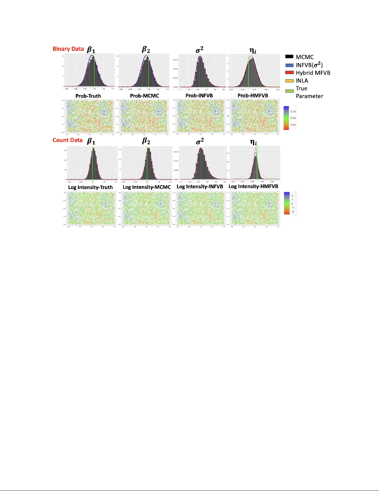
A Scalable V ariational Ba y es Approac h to Fit High-dimensional Spatial Generalized Linear Mixed Mo dels Jin Hyung Lee Departmen t of Statistics, George Mason Universit y and Ben Seiy on Lee ∗ Departmen t of Statistics, George Mason Universit y Abstract Gaussian and discrete non-Gaussian spatial datasets are common across ﬁelds lik e public health, ecology , geosciences, and social sciences. Ba y esian spatial generalized linear mixed mo dels (SGLMMs) are a ﬂexible class of mo dels for analyzing such data, but they struggle to scale to large datasets. Many scalable Ba yesian methods, built up on basis representations or sparse cov ariance matrices, still rely on p osterior sampling via Marko v chain Mon te Carlo (MCMC). V ariational Ba y es (VB) metho ds ha v e b een applied to SGLMMs, but only for small areal datasets. W e prop ose tw o computationally eﬃcient VB approac hes for analyzing mo derately sized and massiv e (millions of lo cations) Gaussian and discrete non-Gaussian spatial data in the contin uous spatial domain. Our metho ds leverage semi-parametric ap- pro ximations of latent spatial pro cesses and parallel computing to ensure computational eﬃciency . The prop osed metho ds deliver inferential and predictiv e p erformance comparable to gold-standard MCMC methods while achieving computational sp eedups of up to 3600 times. In most cases, our VB approaches outp erform state-of-the-art alternativ es suc h as INLA and Hamiltonian Mon te Carlo. W e v alidate our methods through a comparativ e nu- merical study and applications to real-w orld datasets. These VB approaches can enable practitioners to model millions of discrete non-Gaussian spatial observ ations on standard laptops, signiﬁcan tly expanding access to adv anced spatial mo deling to ols. Keywor ds: Spatial Statistics, V ariational Inference, Remote Sensing, Statistical Computing, Basis Representation, P arallel Computing, Non-Gaussian Spatial Data ∗ Corresp onding Author: slee287@gm u.edu 1 In tro duction Spatially-dep enden t non-Gaussian datasets are prev alen t in many scientiﬁc applications with examples including remotely sensed aerosol optical depth ( W ei et al. , 2019 ) or cloud cov er ( Sengupta and Cressie , 2013 ), counts of bird sp ecies in ecological surveys ( Guan and Haran , 2018 ), and ice thic kness measuremen ts in glaciological studies ( F ret w ell et al. , 2013 ). Modern data collection mec hanisms hav e led to exp onential gro wth of these datasets with ov er millions of observ ation locations. In addition, these datasets exhibit complex spatial dep endencies, whic h can b e non-stationary o ver heterogeneous spatial domains. Spatial generalized linear mixed mo dels (SGLMMs) ( Diggle , 1998 ; Zhang , 2002 ) are a ﬂex- ible class of mo dels amenable to b oth Gaussian and many non-Gaussian spatial observ ations. SGLMMs model the random e ﬀects as realizations from a latent Gaussian pro cess (GP) with a spatial co v ariance function. Within the Ba yesian hierarchical modeling framework, statisti- cal inference pro ceeds b y sampling from the p osterior distributions using Marko v Chain Mon te Carlo (MCMC), whic h can b e prohibitive when: (i) the latent v ariables are high-dimensional; (ii) spatial pro cess mo dels require costly multiv ariate Gaussian densit y ev aluations; and (iii) the hea vily cross-correlated spatially dep endent random eﬀects lead to slo w mixing Mark ov c hains. F or a review of existing approaches for Gaussian spatial data, please see Bradley et al. ( 2016 ) and Heaton et al. ( 2018 ). Scalable metho ds hav e b een dev elop ed, but ev en these ha ve limitations. Conjugate metho ds ( Bradley et al. , 2020 ; Polson et al. , 2013 ; Alb ert and Chib , 1993 ; De Oliv eira , 2000 ) emplo y eﬃcien t Gibbs samplers but still require MCMC-based p osterior sampling. Integrated nested Laplace Approximations (INLA) ( Rue et al. , 2009 ), in conjunction with sto chastic partial dif- feren tial equations ( Lindgren et al. , 2011 ), provides appro ximations of the marginal p osterior 1 distributions, but it can underestimate the uncertaint y in estimation and predictions ( F erk- ingstad and Rue , 2015 ) and assumes normalit y of the approximate distributions ( Han et al. , 2013 ). The V ecc hia-Laplace appro ximation ( Zilb er and Katzfuss , 2021 ) b ypasses sampling b y using a Laplace approximation of the latent spatial random eﬀects, but it is restricted to para- metric cov ariance functions and mo derately large datasets ( N = 250 k ). V ariational Ba yes (VB) ( Blei and Jordan , 2006 ; Blei et al. , 2017 ; Jordan et al. , 1999 ) ap- proac hes approximate the p osterior distribution using a v ariational function that minimizes the Kullbac k-Leibler (KL) div ergence b etw een a itself and the p osterior. Mean Field V ariational Ba yes (MFVB) ( Blei and Jordan , 2006 ), h ybrid MFVB metho ds ( W ang and Blei , 2013 ; T ran et al. , 2021 ) and Integrated non-factorized v ariational Bay es (INFVB) ( Han et al. , 2013 ) are p opular v arian ts of VB that can scale to larger datasets. T o the best of our knowledge, only a few studies hav e extended VB metho ds to non-Gaussian SGLMMs for areal spatial data, and none hav e tac kled massive non-Gaussian p oint-referenced spatial datasets in the contin uous spatial domain. Ren et al. ( 2011 ) prop ose a VB approach to ﬁt a Gaussian spatial random eﬀects mo del in the con tinuous spatial domain, but these do not scale to larger datasets. W u ( 2018 ) employs INFVB to accurately quantify the p osterior v ariances; how ever, the prop osed approaches apply to a narro w class of Gaussian spatial mo dels on the discrete spatial domain (areal). Similarly , Song et al. ( 2022 ) examines Gaussian spatial data on a graph structure. Bansal et al. ( 2021 ) and P ark er et al. ( 2022 ) mo del coun t and binary areal spatial datasets using Poly´ a Gamma mixtures to exploit conjugacy and b ypass exp ensiv e expectations. Park er et al. ( 2022 ) utilizes a pro duct-form MFVB, whic h can lead to sev ere underestimation of the p osterior v ariances. Bansal et al. ( 2021 ) emplo ys INFVB, yet their approac hes apply to a narrow class of spatial data — areal count data observed at a small 2 n umber of lo cations. W e propose a computationally-eﬃcien t VB approac h for modeling massiv e Gaussian and dis- crete non-Gaussian datasets within the contin uous spatial domain. Our metho d is speciﬁcally tailored for SGLMMs, where the spatial random eﬀects are either mo deled as Gaussian pro- cesses with parametric cov ariance functions (full-SGLMMs) or spatial basis expansions (basis- SGLMMs). As far as w e are aw are, this study represents the ﬁrst attempt to dev elop a scalable v ariational Bay es metho ds or mo deling massive non-Gaussian spatial datasets ( N > 1 × 10 4 ) within the con tinuous spatial domain. F urthermore, we include an extensiv e comparative analy- sis of our prop osed VB approaches, MCMC algorithms, and INLA across a wide arra y of spatial datasets. A piv otal asp ect of our prop osed metho dology is its accessibility to non-exp erts, fa- cilitating easy ﬁne-tuning of SGLMMs to suit their preferences (e.g., incorp orating/excluding co v ariates, modifying co v ariance functions, or adjusting spatial basis functions). W e provide an o verview of SGLMMs in Section 2. W e discuss v ariational Bay es metho ds in Section 3 and in tro duce our prop osed VB approaches in Section 4. A comparativ e analysis is then p erformed across m ultiple comp eting metho ds using n umerical studies (Section 5) and real data examples (Section 6). Finally , Section 7 pro vides a summary of the study , discusses limitations, and prop oses directions for future research. 2 Spatial Generalized Linear Mixed Mo dels (SGLMMs) Spatial generalized linear mixed mo dels (SGLMMs) ( Diggle , 1998 ) are a highly ﬂexible class of spatial mo dels that can accommo date non-Gaussian observ ations, such as binary ( Hanks et al. , 2015 ), count ( Guan and Haran , 2018 ) and p ositiv e-v alued con tin uous data ( Zilber and Katzfuss , 2021 ). Let Z = { Z ( s i ) } N i =1 denote the observ ations collected at lo cations s i ∈ S ⊆ R 2 and 3 X ∈ R N × p b e the matrix of the corresponding cov ariates. Spatial dep endence is often induced through the spatial random eﬀects ω = { ω ( s i ) } N i =1 ∈ R N , which can b e mo deled as a zero-mean Gaussian Pro cess with co v ariance function C (Ψ) and the asso ciated cov ariance parameters Ψ. F or a ﬁnite set of lo cations, the spatial random eﬀects ω follo w a multiv ariate normal distribution ω ∼ N ( 0 , Σ (Ψ)) with cov ariance matrix Σ (Ψ) ⊂ R N × N suc h that Σ (Ψ) ij = C (Ψ) ij for lo cations s i and s j . A p opular class of stationary and isotropic co v ariance function is the Mat´ ern class ( Stein , 1999 ) with co v ariance parameters Ψ = { σ 2 , ϕ, ν } (see supplement for details). F or SGLMMs, the resulting Ba yesian hierarchical mo del is: Data Mo del: Z | η ∼ F ( · | η ) g ( E [ Z | β , ω ]) := η = X β + ω Pro cess Mo del: ω | Ψ ∼ N ( 0 , Σ (Ψ)) (1) P arameter Mo del: β ∼ p ( β ) , Ψ ∼ p (Ψ) . where F ( · ) is a v alid probability distribution (e.g., Benoulli for binary data, Poisson for coun ts), g ( · ) is the link function, η is the linear predictor and p ( β ) and p (Ψ) denote the prior distribu- tions for β and Ψ, resp ectively . W e infer the unkno wn parameter sets β and Ψ as w ell as the N -dimensional spatial random eﬀects ω by obtaining the p osterior distribution π ( β , Ψ , ω | Z ), whic h is not typically a v ailable in analytical form. Hence, π ( β , Ψ , ω | Z ) is commonly appro xi- mated using a sampling-based approac h suc h as MCMC. Fitting SGLMMs to large datasets (i.e., N > 1 × 10 4 ) can be computationally prohibitive due to rep eated op erations on large matrices and inferring the highly-correlated and N -dimensional spatial random eﬀects ω . T o illustrate, the pro cess mo del in (1) requires ev aluating | Σ (Ψ) | and Σ (Ψ) − 1 with costs scaling at O ( 1 3 N 3 ). Next, the high-dimensional and highly correlated 4 ω can result in slow-mixing Marko v c hains in MCMC ( Haran et al. , 2003 ; Raftery , 1996 ) and diﬃculties inferring all N random v ariables. 2.1 Basis Representations T o ﬁt SGLMMs on large spatial datasets, basis expansions hav e b een used to approximate the laten t spatial random pro cesses ( Cressie , 2015 ; Cressie et al. , 2022 ), particularly for non- Gaussian spatial data ( Sengupta and Cressie , 2013 ; Bradley et al. , 2016 ; Lee and Haran , 2022 ; Lee and Park , 2023 ). The laten t spatial random pro cess { ω ( s i ) } N i =1 is appro ximated by a linear com bination of m spatial basis functions { Φ j ( s ) } m j =1 . Sp eciﬁcally , ω ≈ Φ δ with N × m basis functions matrix Φ =  Φ 1 Φ 2 · · · Φ m  whic h consists of basis functions Φ j ∈ R N with comp onen ts corresp onding to eac h location s i and basis co eﬃcients δ ∈ R m . The Bay esian hierarchical mo del for basis representation SGLMMs (basis-SGLMMs) is: Data Mo del: Z | η ∼ F ( · | η ) g ( E [ Z | β , δ ]) := η = X β + Φ δ Pro cess Mo del: δ | ζ ∼ N ( 0 , Σ ( ζ )) (2) P arameter Mo del: β ∼ p ( β ) , ζ ∼ p ( ζ ) where Σ ( ζ ) is the prior co v ariance matrix for the basis co eﬃcients δ with co v ariance parameters ζ . One example is the independent and identically distributed case where Σ ( ζ ) = Diag m ( τ 2 ) and ζ = τ 2 . T o complete the hierarchical mo del, we sp ecify a prior distribution for ζ ∼ p ( ζ ). Since δ ∈ R m where m << N , basis represen tations oﬀer substan tial dimension reduction and con- siderably decrease the computational ov erhead. Additionally , the design of the basis functions Φ j can help reduce correlation in the estimable basis coeﬃcients δ , resulting in faster-mixing 5 Mark ov chains ( Haran et al. , 2003 ). A wide array of spatial basis functions hav e b een explored in the literature, including bi-square (radial) basis functions ( Cressie and Johannesson , 2008 ; Nyc hk a et al. , 2015 ; Katzfuss , 2017 ), empirical orthogonal functions ( Cressie , 2015 ), wa velets ( Nyc hk a et al. , 2002 ), and multiresolution basis functions ( Nychk a et al. , 2015 ; Katzfuss , 2017 ). Although the dimension reduction ach iev ed through the basis represen tation signiﬁcantly impro ves computational eﬃciency , MCMC metho ds are still required to sample from the p os- terior distributions π ( β , ζ , δ | Z ). The dominating cost of basis-SGLMMs is the matrix-v ector m ultiplication Φ δ whic h incurs O ( N m ) in costs. Therefore, MCMC can b e computationally prohibitiv e for cases with large N (observ ations in the millions) and large m (basis functions). 3 V ariational Inference V ariational Bay es (VB) metho ds approximate a p osterior distributions by optimizing a simpler tractable distribution (v ariational function) to b e close to the target. F or a family of distribu- tions Q , VB metho ds select a distribution q ∗ ( θ ) ∈ Q that minimizes the Kullbac k-Leibler (KL) div ergence ( Jordan et al. , 1999 ; Blei and Jordan , 2006 ) to a target function like the p osterior p ( θ | Z ) such that q ∗ ( θ ) = argmin q ∈ Q KL( q || p ( θ | Z )). The KL div ergence is: KL( q || p ( θ | Z )) = E q h log q ( θ ) p ( θ | Z ) i = − Z q ( θ ) log p ( Z | θ ) · p ( θ ) q ( θ ) d θ + log p ( Z ) . (3) Since the KL divergence is alw ays non-negativ e, minimizing KL( q || p ( θ | Z )) is equiv alent to max- imizing the low er b ound on log p ( Z ), or the Evidence Lo w er Bound (ELBO): E LB O ( q ) := Z q ( θ )log p ( Z | θ ) · p ( θ ) q ( θ ) d θ = E q  log p ( Z | θ ) · p ( θ ) q ( θ )  . (4) 6 Tw o c hallenges include: (1) sp ecifying the family for the v ariational function q ∗ ( θ ) and (2) implemen ting distributional constrain ts ( T ran et al. , 2021 ). Without an y constraints, the v ari- ational function that minimizes the KL div ergence is merely the posterior p ( θ | Z ), whic h is in itself in tractable. In this study , we fo cus on three VB approaches - mean ﬁeld v ariational Bay es (MFVB), Hybrid MFVB, and in tegrated non-factorized v ariational Bay es (INFVB). Mean Field V ariational Ba yes (MFVB) Mean Field V ariational Bay es (MFVB) ( W ain- wrigh t et al. , 2008 ) constrains the v ariational function b y imp osing a pro duct form for q . Here, q ∗ ( θ ) = Q L l =1 q ( θ l ) with parameter partitions θ = ( θ 1 , ..., θ L ) ′ . The function that minimizes KL( q ( θ l ) || p ( θ l )) is ( Ormero d and W and , 2010 ): q l ( θ l ) ∝ exp n E θ − l h log p ( θ l | Z , θ ) io , (5) where E θ − l denotes the exp ectation with resp ect to all other v ariables except θ l . The pro duct- form v ariational function q ∗ ( θ θ θ ) is obtained b y cycling through all θ l using a co ordinate ascent- t yp e algorithm ( Bishop , 2006 ; T ran et al. , 2021 ). Ho wev er, the MFVB approach is sub ject to four key limitations. First, the pro duct form (5) assumes independence across the parameter partitions θ θ θ , whic h can lead to p o or appro ximations of the p osterior. Second, conjugacy in θ l is often needed to obtain an analytical form for q ( θ l ). V ariational inference can b e diﬃcult to deriv e for non-conjugate mo dels b ecause the form in (5) ma y not corresp ond to a known parametric family of distributions. Third, the MFVB approac h ma y result in a v ariational function that drastically underestimates b oth the posterior and p osterior predictive v ariances ( Blei and Jordan , 2006 ; Han et al. , 2013 ; Blei et al. , 2017 ), which can result in o verconﬁden t predictions. Finally , the ﬁrst moments in (5) may not b e a v ailable 7 in closed form, which necessitates exp ensive Monte Carlo-based approximations. Within the con text of SGLMMs, these include E [Σ(Ψ) − 1 | ] or E [log | Σ(Ψ) | ] for large cov ariance matrices. Hybrid MFVB, or ﬁxed form v ariational Ba yes (FFVB) ( Salimans and Knowles , 2013 ), ex- tends MFVB to nonconjugate cases ( W ang and Blei , 2013 ). Since the parametric family for q l ( θ l ) is unknown, q ( θ l ) can b e set as m ultiv ariate normal distribution using either Laplace ap- pro ximations or the delta metho d. Despite its ﬂexibilit y , Hybrid MFVB ma y b e computationally prohibitiv e for mo dels with man y unknown parameters. In tegrated Nonfactorized V ariational Ba yes (INFVB) In tegrated Nonfactorized V ari- ational Ba y es (INFVB) is an alternative VB approac h that pro vides accurate representation s of p osterior v ariance ( Han et al. , 2013 ) and reduces computational w alltimes via parallelized computing. Note that MFVB imposes p osterior indep endence constraints (5), whic h can lead to underestimating p osterior v ariances in the presence of strong inter-block relationships ( Blei and Jordan , 2006 ; Han et al. , 2013 ). INFVB relaxes the constraints of this pro duct form ( Han et al. , 2013 ; W u , 2018 ; Bansal et al. , 2021 ) by constructing a v ariational function based on a disjoin t parameter space θ = ( θ θ θ c , θ θ θ d ) ′ resulting in the v ariational function q INFVB ( θ ) = q ( θ c | θ θ θ d ) q ( θ θ θ d ). Replacing q ( θ ) with q INFVB ( θ ) in (3) results in the following (see supplement S.1 for deriv ations): q ∗ INFVB ( θ ) = argmin q INFVB Z q ( θ d )  Z q ( θ c | θ d )log q ( θ c | θ d ) p ( θ c , θ d | Z ) d θ c + log q ( θ d )  d θ d . (6) Due to the double integrals, the ob jectiv e function in (6) can b e diﬃcult to optimize directly ( Han et al. , 2013 ; W u , 2018 ). T o address this, the parameter sets can b e discretized as θ d = { θ (1) d , θ (2) d · · · θ ( J ) d } in (6) where j ∈ (1 , 2 , ..., J ) denotes the indices for the discretized v alues with J b eing the total num b er of discretized p oints. P artitioning the parameter space yields 8 the j -conditional Evidence Lo wer Bounds (ELBOs) given θ ( j ) d ( Han et al. , 2013 ): E LB O ( j ) : ≈ Z q ( θ c | θ ( j ) d )log p ( Z | θ c , θ ( j ) d ) · p ( θ c , θ ( j ) d ) q ( θ c | θ ( j ) d ) d θ c = E q ( θ c | θ ( j ) d ) " log p ( Z | θ c , θ ( j ) d ) · p ( θ c , θ ( j ) d ) q ( θ c | θ ( j ) d ) # (7) The v ariational functions for q ( θ d ) and q ( θ c ) are approximated using weigh ted a v erages of the conditional v ariational functions q ( θ c | θ ( j ) d ) and the discretized function q ( θ ( j ) d ). The corresp onding normalized w eigh ts are A j = E LB O ( j ) P J j =1 E LB O ( j ) with the j -th conditional E LB O ( j ) from (7). Speciﬁcally , q ( θ d ) is obtained b y m ultiplying A j with the empirical distribution 1( θ d = θ ( j ) d ). Similarly , q ( θ c ) is acquired b y multiplying A j with q ( θ c | θ ( j ) d ) as follows: q ( θ c ) = J X j =1 A j q ( θ c | θ ( j ) d ) , q ( θ d ) = J X j =1 A j 1( θ d = θ ( j ) d ) where A j = E LB O ( j ) P J j =1 E LB O ( j ) (8) Figure 1 provides an ov erview of the INFVB w orkﬂow and additional details for the INFVB pro cedure and algorithms are pro vided in the supplemen t. Figure 1: W orkﬂow diagram of In tegrated Non-F actorized V ariational Bay es (INFVB). 9 4 Our Approac h: V ariational Inference for SGLMMs In this section, we prop ose tw o VB approac hes for ﬁtting SGLMMs. The ﬁrst approach mo dels the laten t spatial pro cess ω as a stationary isotropic Gaussian pro cess (full-SGLMM), consistent with traditional spatial modeling tec hniques, while the second approach utilizes basis expansions (basis-SGLMM) to enable scalabilit y to massiv e datasets. 4.1 F ull Spatial Generalized Linear Mixed Mo dels (full-SGLMM) Consider the full-SGLMM (1) with the option of using one of three data mo dels: Data Model: (Gaussian) Z | β , ω , τ 2 ∼ N ( X β + ω , τ 2 I ) (P oisson) Z | λ ∼ P ois( λ ) where λ = exp( X β + ω ) (Binary) Z | p ∼ Bern( p ) where p = (1 + exp {− X ′ β − ω } ) − 1 Pro cess Mo del: ω | σ 2 , ϕ ∼ N ( 0 , σ 2 R ϕ ) P arameter Mo del: β ∼ N ( µ β , Σ β ) τ 2 ∼ IG( α τ , β τ ) σ 2 ∼ IG( α σ , β σ ) ϕ ∼ p ( ϕ ) Here, Σ (Ψ) in (1) b ecomes σ 2 R ϕ where σ 2 > 0 is the partial sill, R ϕ is the spatial correlation matrix parameterized by ϕ , the range parameter in Mat ´ ern class that gov erns the deca y in spatial dep endence with resp ect to distance. W e prop ose tw o INFVB approac hes diﬀering in the choice of discretized parameter sets, sp eciﬁcally θ θ θ d = ϕ and θ θ θ d = ( ϕ, σ 2 ) ′ . In the ﬁrst case ( θ θ θ d = ϕ ), w e b egin b y grouping γ = ( β , ω ) ′ to a v oid underestimating the p osterior v ariances, which often o ccur in the pro duct-form v ariational function ( Blei et al. , 2017 ). Next, the parameter space is partitioned into tw o comp onents: θ θ θ c = { γ , σ 2 } (or θ θ θ c = { γ , σ 2 , τ 2 } for the Gaussian data mo del) and θ θ θ d = ϕ . W e discretize θ d = { θ (1) d , θ (2) d · · · θ ( J ) d } on a user-sp eciﬁed grid with J 10 p oin ts. F or eac h θ ( j ) d , w e separately p erform MFVB on the parameter blo cks within θ c . F or the j -th partition, initial v alues for E LB O ( j ) 0 , q 0 ( γ | θ ( j ) d ), q 0 ( σ 2 | θ ( j ) d ), and q 0 ( τ 2 | θ ( j ) d ) are set. Then the INFVB algorithm proceeds un til it meets the stopping criterion | E LB O ( j ) k − E LB O ( j ) k − 1 | < ϵ ∗ for a ﬁxed threshold ϵ ∗ . Finally , the weigh ted v ariational functions q ( γ ), q ( σ 2 ), q ( τ 2 ), and q ( ϕ ) are computed using ELBO weigh ts A j . Additional details for constructing and up dating the v ariational functions q ( · ) are pro vided in the following subsection. A multiv ariate normal prior distribution is selected for γ = ( β , ω ) ′ where γ ∼ N ( µ γ , Σ γ ) and µ γ = ( µ β , 0 ) ′ and Σ γ =     Σ β 0 0 σ 2 R ϕ     , σ 2 ∼ IG( α σ , β σ ), and τ 2 ∼ IG( α τ , β τ ). Discretization for the parameters in θ d should b e reﬂectiv e of the resp ectiv e prior distributions (details pro vided in Section 4.3). The general INFVB mo del-ﬁtting pro cedure is outlined in Algorithm 1. An extension using t wo discretized parameters θ θ θ d = ( ϕ, σ 2 ) ′ (Algorithm S.1) is provided in the supplemen t. Algorithm 1 INFVB( ϕ ) Algorithm for full-SGLMMs Initialize Set ϵ ∗ and discr etize { ϕ (1) d , ϕ (2) d , ..., ϕ ( J ) d } for user-sp e ciﬁe d J . for j=1,...,J do Initialize Set E LB O ( j ) 0 , q 0 ( γ | ϕ ( j ) d ) , q 0 ( σ 2 | ϕ ( j ) d ) and k = 1 while | E LB O ( j ) k − E LB O ( j ) k − 1 | > ϵ ∗ do Up date q k ( γ | ϕ ( j ) d ) Up date q k ( σ 2 | ϕ ( j ) d ) Up date E LB O ( j ) k k ← k + 1 end Set q ( γ | ϕ ( j ) d ) = q k ( γ | ϕ ( j ) d ) , q ( σ 2 | ϕ ( j ) d ) = q k ( σ 2 | ϕ ( j ) d ) end Result Weighte d Non-factorize d V ariational F unctions 1. A j = E LB O ( j ) P J i =1 E LB O ( i ) 2. q ( γ ) = Σ J j =1 A j q ( γ | ϕ ( j ) d ) 3. q ( σ 2 ) = Σ J j =1 A j q ( σ 2 | ϕ ( j ) d ) 4. q ( ϕ ) = Σ J j =1 A j 1( ϕ d = ϕ ( j ) d ) 11 V ariational F unctions for Gaussian, P oisson, and Bernoulli Data Mo dels F or Gaus- sian data mo dels, conditional conjugacy exists for β , ω and σ 2 ; in addition, the ω can b e in tegrated out to reduce the n umber of estimable parameters. Hence, the v ariational functions q ( γ | θ ( j ) d ) and q ( σ 2 | θ ( j ) d ) are av ailable in closed form (see supplement). On the other hand, SGLMMs with Poisson and Bernoulli data models do not b eneﬁt from conditional conjugacy for γ , whic h can b e problematic for obtaining the exp ectations in q ( σ 2 ) ∝ E γ [log( p ( γ , σ 2 , Z )] and the E LB O . Monte Carlo metho ds can provide n umerical appro ximations for these expectations; ho wev er, these metho ds can b e costly as their accuracy relies on the num b er of Monte Carlo samples. In this study , w e appro ximate q ( γ ) using a Laplace appro ximation ( W ang and Blei , 2013 ) for P oisson data mo dels and auxiliary v ariable metho ds ( Jaakkola and Jordan , 1997 ; Park er et al. , 2022 ) for Bernoulli data mo dels. Due to space limitations, details for these approximations are provided in the supplement. 4.2 V ariational Metho d for Basis-Represen tation Mo dels The Ba yesian hierarchical mo del for basis-SGLMMs (2) is provided b elo w and the accompanying VB algorithms are pro vided in the supplement (Algorithms S.2 and S.3). Data Model: (Gaussian) Z | β , δ , τ 2 ∼ N ( X β + Φ δ , τ 2 I ) (P oisson) Z | λ ∼ P ois( λ ) where λ = exp( X β + Φ δ ) (Binary) Z | p ∼ Bern( p ) where p = (1 + exp {− X ′ β − Φ δ } ) − 1 Pro cess Mo del: δ | σ 2 ∼ N (0 , σ 2 Σ δ ) P arameter Mo del: β ∼ N ( µ β , Σ β ) , τ 2 ∼ IG( α τ , β τ ) , σ 2 ∼ IG( α σ , β σ ) 12 W e assume that the basis functions con tained in Φ are ﬁxed prior to mo del-ﬁtting. Basis- SGLMMs can b e ﬁtted using b oth Hybrid MFVB and INFVB methods, as the only estimable parameters are γ = ( β , δ ) ′ and σ 2 for count and binary data, and additionally τ 2 for Gaussian data, all of whic h hav e amenable v ariational functions. F or the Hybrid MFVB approac h, Al- gorithm S.2 outlines the pro cedural steps. F or initialization, we set q (0) γ , q (0) σ 2 , ϵ ∗ , and E LB O 0 . The Hybrid MFVB algorithm up dates q ( k ) γ and q ( k ) σ 2 iterativ ely un til reaching a stopping crite- rion. Prior distributions are chosen similarly to the full-SGLMM case. Mo diﬁcations for q ( γ ) are needed for count and binary data, akin to the approach outlined in Section 4.1. As in the previous subsection, we employ normal appro ximations for q k ( γ ); for instance, the Laplace Appro ximation for count data models and the quadratic appro ximation ( Jaakk ola and Jordan , 1997 ) for binary data mo dels. The INFVB metho d discretizes θ θ θ d = σ 2 across J partitions θ d = { θ (1) d , θ (2) d · · · θ ( J ) d } . Algorithm S.3 outlines the pro cedure, which results in weigh ted v ari- ational functions q ( γ ) and q ( σ 2 ) from A j . Please see the supplemen t for necessary deriv ations regarding each case (Hybrid MFVB and INFVB for the Poisson and Bernoulli data mo dels). 4.3 Implemen tation Details The prop osed v ariational metho ds include imp ortant tuning parameters. This includes the n umber of p oin ts J for the discretized parameters θ d in INFVB, the spacing of the discretized parameter sets, and the threshold ϵ ∗ for stopping the INFVB and Hybrid MFVB algorithm. In b oth INFVB implementations for full-SGLMMs, w e discretize ϕ into J = 1 , 000 v alues and the parameter pairs ( ϕ, σ 2 ) into J = 10 , 000 v alues. Discretizing σ 2 in INFVB is a non-trivial c hallenge b ecause the inv erse gamma prior distribution does not hav e a ﬁnite upp er b ound. In practice, we suggest implementing b oth the Hybrid MFVB and INFVB approac h in that order. Hybrid MFVB uses few er computational resources and ma y yield similar results to the INFVB 13 approac h in some cases (e.g., basis SGLMMs). How ev er, Hybrid MFVB may underestimate the p osterior v ariances of the mo del parameters and predictions, making INFVB necessary to correctly approximate the p osterior v ariances. F or INFVB, we recommend selecting the b ounds for σ 2 based on the quan tiles from the resulting v ariational function q ( σ 2 ) obtained via Hybrid MFVB. F or q ( σ 2 ), we set the lo wer and upp er b ounds to b e 0 and 2000, resp ectiv ely . INFVB con tains em barrassingly parallel op erations, whic h can b e distributed across multiple pro cessors. W e emplo y ed 30 cores for eac h im plemen tation of INFVB. If p ossible, w e recommend using J cores (i.e., one core p er discretized v alue of θ ( j ) d ). F or basis-SGLMMs, we explored scenarios with 20, 50, and 100 basis functions. Our proposed VB methods are extremely fast; hence, the practitioner can easily test a wide range of bases and select the appropriate mo del. Finally , we set our stopping criterion ϵ ∗ = 1 × 10 − 4 . Increasing the stopping criterion would end the algorithm earlier but may compromise accuracy . W e employ a VB-subsampling approach to estimate the linear predictor for lo cation i , η i = X ′ i β + ω i and η i = X ′ i β + Φ ′ i δ in the full- and basis-SGLMM cases, resp ectively . The subsampling approac h is embarrassingly parallel and yields p osterior distributions comparable to those from MCMC. F urther details are pro vided in the supplementary section S.6. 5 Sim ulation Study W e demonstrate our prop osed VB approaches through a comparativ e sim ulation study that ev aluates m ultiple sim ulated datasets v arying in size, strength of spatial dependence, and data t yp e, including Gaussian, binary , and count data. W e p erform three types of comparative anal- yses: (1) an extensive comparativ e analysis ﬁtting full-SGLMMs on mo derately-large datasets ( N = 500); (2) basis-SGLMMs on large datasets ( N = 25 , 000); and (3) a separate compar- 14 ison b et w een VB-based metho ds and Hamiltonian Monte Carlo (HMC) using the No U-T urn Sampler (NUTS) implemented in RStan . The VB- and MCMC-based are implemen ted on a high-p erformance c omputing infrastructure with walltimes based on a single 2.4 GHz Intel Xeon Gold 6240R processor.INLA w as implemen ted on an Apple MacBook Pro laptop equipp ed with an M1 Pro c hip. 5.1 Case 1: Mo derately-Large Datasets with F ull-SGLMMs Sim ulation Study Design W e randomly select lo cations s i ∈ D = [0 , 1] 2 ⊂ R 2 for i = 1 , . . . , N , where D represents the spatial domain. Eac h dataset consists of N = 500 lo cations divided into N train = 400 for training and N test = 100 for testing. The vector of observ ations Z = ( Z ( s 1 ) , ..., Z ( s N )) T is generated using the SGLMM framew ork in Section 4.1 with co v ariates X = [ X 1 , X 2 ] where X 1 , X 2 ∼ Unif( − 1 , 1) and β = (1 , 1). F our diﬀeren t sets of spatial random eﬀects ω = { ω ( s i ) : s i ∈ D } are generated from a zero-mean Gaussian Pro cess with Mat´ ern co v ariance function with smo othness ν = 0 . 5, partial sill σ 2 = 1, and range parameters ϕ = { 0 . 1 , 0 . 3 , 0 . 5 , 0 . 7 } . W e generate observ ations Z for the Gaussian, binary , and coun t datasets using the identit y , logit, and log link functions, resp ectiv ely . W e generated 50 replicate datasets for eac h of the 12 scenarios. F or this sim ulation study , we compare the tw o prop osed INFVB metho ds, the Metrop olis—Hastings algorithm, and INLA. The INFVB( ϕ ) approac h discretizes only ϕ , whereas INFVB( ϕ, σ 2 ) discretizes t wo parameters ( ϕ, σ 2 ). See Algorithm 1 and S.1 for details. F or MCMC, we obtained 100,000 posterior samples with conv ergence assessed using batch means standard errors (BMSE) ( Flegal et al. , 2008 ) and visual heuristics of trace plots. F or the INFVB methods, w e set the stopping as threshold as ϵ ∗ = 1 × 10 − 4 (see Algorithm 1). Details on discretizations for ϕ and σ 2 are provided in Section 4.3. INLA ( Rue et al. , 2009 ) employs stochastic partial diﬀerential equations ( Lindgren and Rue , 15 2015 ) to deliver numerical Gaussian appro ximations of the marginal p osterior distributions. Implemen tations are done through the R-INLA pack age av ailable at www.r-inla.org . T o complete the hierarchical model (Section 4.1), w e set parameter mo dels (priors) β j ∼ N (0 , 100), τ 2 ∼ IG(0 . 1 , 0 . 1), σ 2 ∼ IG(0 . 1 , 0 . 1) and ϕ ∼ Unif(0 , √ 2). W e ev aluate predictive p erformance using ro ot mean squared prediction error RMSPE = r 1 N test P N test i =1  Z i − ˆ Z i  2 ! for the Gaussian and count data and the area under the receiver op erating characteristic curve (A UC) for the binary case. T o ev aluate interv al inference, w e consider the contin uous rank ed probabilit y score (CRPS) ( Hersbac h , 2000 ) and compute the co verage of the the 95% credible in terv als. The latter represents the frequency with which the 95% credible interv al for the linear predictor encompasses the true linear predictor. Please see supplment for the CRPS and co verage results. Results The results for the binary and count data are summarized in T able 1 and those for the Gaussian case are in the supplement S.1. Our prop osed VI metho ds and MCMC ha v e near-iden tical predictive p erformance (RMSPE and AUC). How ever, the VI-based methods exhibit dramatic computational sp eedups ranging from factors of 340-to-512 for the binary case and 18-to-20 for coun t data. Note that INFVB for count data requires an additional Laplace appro ximation step; hence, the computational speedup is less pronounced than the binary cases. Though INLA exhibits a substan tial computational sp eedup for the full-SGLMM, achieving up to a 3956-fold impro vemen t compared to MCMC-based metho ds (the gold standard), it yields low er AUC for binary data and higher RMSPE for count data. MCMC, INFVB( ϕ ), and INFVB( ϕ, σ 2 ) yield comparable results for CRPS (T able S.3). Despite its computational sp eedup, INLA underp erforms the other approaches in both CRPS and cov erage. F or all datasets, we ﬁnd that the resulting p osterior distributions are similar across the t wo 16 Binary A UC (W alltime in seconds) Sp eedup MCMC INFVB INFVB INLA INFVB INFVB INLA ( ϕ ) ( ϕ, σ 2 ) ( ϕ ) ( ϕ, σ 2 ) ϕ = 0 . 1 0.71 (8097.17) 0.71 (23.81) 0.71 (16.81) 0.68 (2.05) 340.01 481.66 3955.86 ϕ = 0 . 3 0.73 (8097.16) 0.73 (23.79) 0.73 (16.24) 0.68 (2.07) 340.32 498.47 3907.85 ϕ = 0 . 5 0.73 (8116.32) 0.73 (22.86) 0.73 (15.85) 0.68 (2.14) 354.97 511.99 3799.83 ϕ = 0 . 7 0.73 (8105.36) 0.74 (22.22) 0.74 (15.87) 0.70 (2.08) 364.80 510.80 3893.77 Coun t RMSPE (W alltime in seconds) Sp eedup MCMC INFVB INFVB INLA INFVB INFVB INLA ( ϕ ) ( ϕ, σ 2 ) ( ϕ ) ( ϕ, σ 2 ) ϕ = 0 . 1 2.83 (7627.31) 2.82 (418.20) 2.82 (379.11) 3.77 (2.44) 18.24 20.12 3130.47 ϕ = 0 . 3 2.09 (7700.58) 2.09 (414.15) 2.09 (376.14) 3.42 (2.46) 18.59 20.47 3126.23 ϕ = 0 . 5 1.73 (7738.14) 1.72 (408.98) 1.72 (377.15) 2.79 (2.24) 18.92 20.52 3452.81 ϕ = 0 . 7 1.78 (7735.17) 1.78 (391.20) 1.78 (376.14) 2.75 (2.20) 19.77 20.56 3512.51 T able 1: Comparison of RMSPE (W alltime in seconds) and sp eedup for MCMC, INFVB( ϕ ), INFVB( ϕ, σ 2 ), and INLA for the full-SGLMMs case when N = 500. Results for the binary (top) and coun t datasets (bottom) are provided. The rep orted v alues represen t the av erages across all replicate datasets. INFVB metho ds, MCMC and HMC. This is notable b ecause v ariational approaches hav e been critiqued for underestimating p osterior v ariances. Figure 2 includes comparisons of the p osterior distributions for tw o cases - binary and count data using ϕ = 0 . 7. The ﬁgure also displays the p osterior distributions of linear predictors η i and η j corresp onding to randomly selected lo cations i and j . Note that v ariational Ba yes metho ds, namely MFVB, hav e b een kno wn to underestimate p osterior v ariance ( Han et al. , 2013 ; Blei et al. , 2017 ). Ho wev er, our results suggest that the INFVB metho d with tw o parameter discretizations, INFVB( ϕ, σ 2 ), pro vides accurate appro ximations of the true p osterior distributions. While the single-parameter version INFVB( ϕ ) pro vides comparable prediction results, it do es underestimate p osterior v ariances, particularly with the partial sill parameters σ 2 . F or practitioners, we recommend using the INFVB( ϕ, σ 2 ) as it b etter approximates p osterior v ariances while preserving prediction accuracy . Since INLA mo dels the latent surface using sto chastic partial diﬀeren tial equations (SPDE), as opp osed to a full Gaussian pro cess, comparisons of β 1 , β 2 , σ 2 , and ϕ with the other metho ds 17 ma y not b e reliable. How ever, we b elieve that a comparison of the linear predictors η i ’s is fair. Note that the marginal p osterior distributions for η i and η j from INLA diﬀer to those from the other metho ds. Figure 2: F ull-SGLMM: Comparison of p osterior distributions for MCMC (orange), INFVB( ϕ ) (purple), INFVB( ϕ, σ 2 ) (blue), and INLA (red) when ϕ = 0 . 7 and N = 500. Results for the binary (top panel) and coun t datasets (bottom panel) are provided along with the true parameter v alues (black dashed lines). P osteriors are shown for all estimated parameters and t w o chosen linear predictors, η i and η j . INLA is used only for estimating the linear predictor η i , not the other parameters. 5.2 Case 2: Large Datasets with Basis-SGLMMs Sim ulation Design W e randomly select 25,000 lo cations s i ∈ D = [0 , 1] 2 ⊂ R 2 with N train = 20 , 000 lo cations for training and N test = 5 , 000 reserved for v alidation. The cov ariates ( X 1 and X 2 ), mo del parameters ( β , σ 2 ), and spatial random eﬀects ( ω ) are generated similarly as in the previous section. W e emplo y the basis-SGLMM framework outlined in Section 4 . 2 using the 18 appro ximation ω ≈ Φ δ where Φ is an n × m matrix where each column contains a pre-sp eciﬁed spatial eigen basis function. F or this particular implemen tation, the bases are made up of the m -leading eigenv ectors of a Mat´ ern cov ariance function with smo othness ν = 0 . 5, partial sill σ 2 = 1, and the corresp onding range parameters used to generate the data. W e use the leading m = { 20 , 50 , 100 } basis functions (eigenv ectors) in this simulation study . Though basis function sp eciﬁcation is an activ e area of research, incorp orating basis selection lies b eyond the scop e of this study . W e ﬁt the basis-SGLMM mo dels (Section 4 . 2) using four diﬀerent metho ds - Hybrid MFVB (Algorithm S.2), INFVB( σ 2 ) (Algorithm S.3), MCMC and INLA. Parameter mo dels, stopping criteria for the VB metho ds, and MCMC implementation are similar to those in the previous section. Results Out-of-sample prediction accuracy is comparable across all four mo del-ﬁtting ap- proac hes, as sho wn in T able 2 for the binary and coun t datasets using 50-leading eigen vectors. Ho wev er, the VI-based approaches show stark improv ements in computational eﬃciency as ev- idenced by the large computational sp eedup factors (ov er MCMC). F or the binary case, the sp eedup factor ranges from 3527-to-3649 for Hybrid MFVB and 47-to-50.91 for INFVB. F or coun t datasets, the sp eedup factor is around 148-to-162 for Hybrid MFVB and 7-to-8 for IN- FVB. The coun t data cases require an embedded Laplace approximation, whic h explains the w alltime diﬀerences betw een the binary and coun t cases. The computational cost is lo wer for Hybrid MFVB as it requires a single pro cessor to run the Hybrid MFVB algorithm. Ho wev er, the INFVB( σ 2 ) approac h en tails running m ultiple ( J = 1 , 000) procedures across a limited n um- b er of pro cessors (30 total), which detracts from the computational gains. This speedup would b e more pronounced if more computational resources (pro cessors) were a v ailable. INLA oﬀers a similar speedup to INFVB( σ 2 ) with comparable results, though it is slo wer than Hybrid MFVB. 19 F or the binary data, MCMC, Hybrid MFVB, and INFVB( σ 2 ) yield similar CRPS v alues, whereas INLA demonstrates a higher CRPS (T able S.10). In contrast, for cov erage, all ap- proac hes pro duce comparable results. F or the count data, INLA also exhibits a higher CRPS, consisten t with its p erformance on binary data. Ho wev er, INLA achiev es the b est result in co verage, capturing 92% of the true v alues. Binary A UC (W alltime in seconds) Sp eedup MCMC Hybrid INFVB INLA Hybrid INFVB INLA MFVB ( σ 2 ) MFVB ( σ 2 ) ϕ = 0 . 1 0.75 (688.20) 0.75 (0.19) 0.75 (14.33) 0.75 (14.21) 3649.00 48.03 48.44 ϕ = 0 . 3 0.75 (695.70) 0.75 (0.20) 0.75 (14.56) 0.75 (14.02) 3527.19 47.78 49.63 ϕ = 0 . 5 0.74 (691.34) 0.74 (0.19) 0.74 (14.27) 0.74 (14.33) 3590.63 48.45 48.23 ϕ = 0 . 7 0.73 (685.51) 0.73 (0.19) 0.73 (13.46) 0.73 (14.17) 3641.29 50.91 48.37 Coun t RMSPE (W alltime in seconds) Sp eedup MCMC Hybrid INFVB INLA Hybrid INFVB INLA MFVB ( σ 2 ) MFVB ( σ 2 ) ϕ = 0 . 1 2.06 (721.19) 2.06 (4.44) 2.06 (97.09) 2.11 (18.56) 162.26 7.43 38.85 ϕ = 0 . 3 1.37 (708.39) 1.37 (4.74) 1.37 (90.56) 1.38 (15.50) 149.61 7.82 45.71 ϕ = 0 . 5 1.16 (689.52) 1.16 (4.64) 1.16 (85.72) 1.16 (13.99) 148.75 8.04 49.30 ϕ = 0 . 7 1.08 (683.34) 1.08 (4.34) 1.08 (85.07) 1.08 (13.67) 157.37 8.03 49.98 T able 2: Comparison of RMSPE (w alltime in seconds) and a v erage speedup for MCMC, Hybrid MFVB, INFVB( σ 2 ), and INLA for the basis-SGLMM case when using 50 eigen Bases functions. Results for the binary (top) and coun t datasets (bottom) are provided. The reported v alues represen t the a verages across all replicate datasets. Figure 3 compares the relev an t p osterior distributions for tw o cases - binary and count data when ϕ = 0 . 5. The resulting p osterior distributions are nearly identical across all metho ds, including MCMC, INFVB, Hybrid MFVB, and HMC. Since the predictive p erformances are similar, we suggest using the Hybrid MFVB approach for ﬁtting basis-SGLMMs primarily due to its computational eﬃciency . W e also employ INLA and four other metho ds to estimate the linear predictor η . The results app ear comparable for binary data; how ever, for count data, INLA exhibits a larger v ariance. 20 Figure 3: Basis-SGLMM: Comparison of p osterior distributions for MCMC (blac k), INFVB( σ 2 ) (blue), Hybrid MFVB (red), and INLA (orange) for the case when ϕ = 0 . 5 and N = 25 k . Results for the binary (top panel) and count datasets (b ottom panel) are pro vided. Posteriors shown for mo del parameters and linear predictor η i . INLA is used only for estimating the linear predictor η i , not the other parameters. T rue and predicted latent probabilit y (binary) and log intensit y (coun t) are pro vided for all four methods. 5.3 Case 3: Comparison with Scalable Metho ds (INLA and HMC) W e ev aluate the prop osed VB metho ds to INLA and tw o MCMC algorithms (Metrop olis— Hastings and HMC) through an abridged simulated example. The purp ose of this separate analysis is to compare the VB approach (predictions and walltimes) to a more eﬃcient MCMC sampler such as HMC. W e generate data for b oth the full and basis-SGLMMs as in the previous subsections. The spatial random eﬀects ω come from a zero-mean Gaussian process with Mat´ ern co v ariance function parameterized by ν = 0 . 5, σ 2 = 1, and m ultiple spatial range parameters ϕ = { 0 . 1 , 0 . 3 , 0 . 5 , 0 . 7 } . W e use a total of 16 sim ulated datasets corresp onding to the spatial mo del (full vs. basis-SGLMM), data type (count vs. binary), and spatial range parameters. 21 Binary AUC (W alltime in seconds) Speedup MCMC INFVB INFVB INLA HMC INFVB INFVB INLA HMC ( ϕ ) ( ϕ, σ 2 ) ( ϕ ) ( ϕ, σ 2 ) ϕ = 0 . 1 0.68 (7840.70) 0.67 (24.80) 0.67 (20.06) 0.66 (2.09) 0.69 (1561.60) 316.11 390.78 3748.22 5.02 ϕ = 0 . 3 0.77 (7796.61) 0.77 (18.61) 0.77 (17.01) 0.68 (2.08) 0.79 (1279.33) 418.88 458.49 3755.79 6.09 ϕ = 0 . 5 0.70 (8553.98) 0.70 (29.63) 0.70 (15.96) 0.65 (2.17) 0.70 (1263.89) 288.69 535.93 3936.04 6.77 ϕ = 0 . 7 0.74 (8577.10) 0.73 (27.14) 0.73 (15.55) 0.71 (2.07) 0.75 (1109.72) 316.05 551.65 4141.94 7.73 Count RMSPE (W alltime in seconds) Speedup MCMC INFVB INFVB INLA HMC INFVB INFVB INLA HMC ( ϕ ) ( ϕ, σ 2 ) ( ϕ ) ( ϕ, σ 2 ) ϕ = 0 . 1 1.97 (7468.93) 1.96 (419.96) 1.96 (436.53) 2.25 (2.25) 1.98 (63.02) 17.78 17.11 3316.65 118.51 ϕ = 0 . 3 2.89 (7635.57) 2.90 (406.64) 2.90 (376.93) 4.95 (2.48) 2.90 (106.12) 18.78 20.26 3083.21 71.95 ϕ = 0 . 5 0.99 (7566.05) 0.99 (364.73) 0.99 (371.47) 1.25 (2.08) 0.93 (86.57) 20.74 20.37 3641.89 87.40 ϕ = 0 . 7 1.99 (7571.67) 1.98 (477.54) 1.98 (369.49) 2.27 (2.18) 2.03 (93.25) 15.86 20.49 3473.50 81.20 T able 3: Comparison of RMSPE (w alltime in seconds) and sp eedup for MCMC, INFVB( ϕ ) INFVB( ϕ, σ 2 ), INLA and HMC for the full-SGLMM case. Results for the binary (top) and coun t datasets (b ottom) are provided. Results from this comparativ e analysis (T ables 3 and 4) sho w that VB-based metho ds obtain comparable prediction and inferen tial results as the MCMC-based metho ds, but at a fraction of the time. Although INLA is faster than our approac hes in the full-SGLMM case, it results in lo wer AUC for binary data and higher RMSPE for count data. F or basis-SGLMMs, INLA has comparable predictiv e p erformance to the VB-based approac hes, but has longer mo del-ﬁtting w alltimes than the Hybrid MFVB case. HMC, implemen ted through the RStan pac k age ( Carp en ter et al. , 2017 ), produces rapidly mixing Marko v chains with relatively large eﬀective sample sizes with resp ect to the num b er of iterations. Hence, HMC requires signiﬁcantly few er samples than the Metropolis—Hastings algorithm ( Betancourt , 2017 ) to obtain comparable eﬀective sample sizes. HMC p erforms simi- larly to the Metrop olis—Hastings and VB-based approac hes in prediction, but has longer wall- times. HMC’s slow er walltimes can b e attributed to its generation of near-indep enden t samples with larger eﬀective sample sizes. Though the Metrop olis—Hastings algorithm has a faster p er- iteration runtime compared to HMC, it do es not generate nearly as man y indep endent samples 22 Binary AUC (W alltime in seconds) Speedup MCMC Hybrid INFVB INLA HMC Hybrid INFVB INLA HMC MFVB ( σ 2 ) MFVB ( σ 2 ) ϕ = 0 . 1 0.74 (610.94) 0.74 (0.20) 0.74 (14.34) 0.74 (14.19) 0.74 (919.05) 3133.04 42.60 43.05 0.66 ϕ = 0 . 3 0.75 (606.96) 0.75 (0.20) 0.75 (14.87) 0.75 (14.51) 0.75 (837.21) 2989.93 40.83 41.84 0.72 ϕ = 0 . 5 0.75 (601.01) 0.75 (0.18) 0.75 (13.65) 0.75 (14.36) 0.75 (1035.62) 3357.60 44.04 41.85 0.57 ϕ = 0 . 7 0.73 (597.83) 0.73 (0.20) 0.73 (14.19) 0.73 (13.65) 0.73 (993.30) 3034.69 42.12 43.78 0.60 Count RMSPE (W alltime in seconds) Speedup MCMC Hybrid INFVB INLA HMC Hybrid INFVB INLA HMC MFVB ( σ 2 ) MFVB ( σ 2 ) ϕ = 0 . 1 2.13 (661.12) 2.13 (4.36) 2.13 (100.71) 2.16 (18.28) 2.13 (899.49) 151.77 6.56 36.17 0.73 ϕ = 0 . 3 1.34 (653.53) 1.34 (4.68) 1.34 (97.52) 1.35 (15.55) 1.34 (931.09) 139.52 6.70 42.03 0.70 ϕ = 0 . 5 1.19 (655.06) 1.19 (4.76) 1.19 (87.16) 1.19 (13.36) 1.19 (932.24) 137.65 7.52 49.02 0.70 ϕ = 0 . 7 1.09 (645.05) 1.08 (4.42) 1.08 (86.12) 1.08 (14.76) 1.08 (909.79) 145.94 7.49 43.70 0.71 T able 4: Comparison of RMSPE (walltime in seconds) and sp eedup for MCMC, Hybrid MFVB, INFVB( σ 2 ) and HMC for the basis-SGLMM case when using 50 basis functions. Results for the bi- nary (top) and count datasets (b ottom) are provided. as evidenced by the smaller eﬀective sample sizes. On the other hand, HMC’s w alltimes are considerably slow er than those for the VB-based approaches and has m uc h smaller eﬀective sample sizes. Note that the VB-based metho ds generate indep endent samples from the v aria- tional distributions, which provides a clear adv antage (e.g. higher eﬀective sample sizes) ov er the auto-correlated samples from MCMC. 6 Application In this study , we apply our approach to tw o large spatial en vironmental datasets. The ﬁrst application sho w cases the dramatic scalability of our VI-based approach by mo deling a massiv e spatial binary dataset ( N =2.7 million) deriv ed from remotely sensed satellite imagery . A second case that fo cuses on a large spatial coun t dataset is provided in the supplemen t S.8. As the ﬂagship mission of the Earth Observing System, the National Aeronautics and Space Administration (NASA) launc hed the T erra Satellite in Decem b er 1999. Similar to past studies ( Sengupta and Cressie , 2013 ; Bradley et al. , 2016 ; Lee and Haran , 2022 ), we mo del the cloud 23 mask data captured b y the Mo derate Resolution Imaging Sp ectroradiometer (MODIS) instru- men t onboard the T erra satellite. The spatial binary resp onses Z ( s ) ∈ { 0 , 1 } represent the presence/absence of cloud mask at 1 k m spatial resolutions. The data consists of n = 2 , 748 , 620 lo cations where 90% is used to ﬁt the mo del and 10% reserv e d for v alidation. Since the cloud mask data is binary and massiv e in size, w e emplo y the basis-SGLMM mo del (Section 4.2) with a logit link function. The Moran’s eigen basis functions ( Lee and Haran , 2022 ) are used for this application. As done in past studies ( Sengupta and Cressie , 2013 ; Bradley et al. , 2016 ; Lee and Haran , 2022 ), we use the v ector 1 and the v ector latitudes as co v ariates. W e compare the Hybrid MFVB and MCMC-based approac hes using maxim um absolute error (MAE), area under the ROC curve (AUC), and the asso ciated w alltimes. W e ﬁt eight diﬀerent basis-SGLMM mo dels for v arious sets of PICAR basis functions. See ( Lee and Haran , 2022 ) for additional details on constructing these basis functions. F or each set, we c hose the leading m basis functions where m ∈ { 25 , 50 , 75 , 100 , 125 , 150 , 175 , 200 } . T able 5 includes a summary of the results and Figure 4 provides spatial maps of the predicted probability surfaces for a subset of the basis function sets. Results indicate that the Hybrid MFVB approach ac hieves near-iden tical predictive p erformance to the MCMC-based approac h with resp ect to AUC and MAE, alb eit at a mere fraction of the computational cost. As exp ected, the prediction accuracy is directly correlated with m , the n um b er of basis functions, since including more basis functions can help capture the high-frequency b ehavior of the latent spatial surfaces. How ever, increasing m also incurs larger computational costs resulting in longer walltimes. The Hybrid MFVB approach exhibits exceptional p ortability as it enables practitioners to mo del millions of non-Gaussian spatial observ ations within a matter of minutes-to-hours, even on a laptop. Our prop osed metho dology delivers results that are on par with MCMC while 24 A UC MAE W alltime (min utes) # Bases VB MCMC VB MCMC VB MCMC Speedup 25 0.82 0.821 0.306 0.305 0.9 858.4 1008 50 0.839 0.839 0.291 0.29 1.1 992.7 882 75 0.853 0.854 0.28 0.279 2.6 1118.6 427 100 0.862 0.862 0.271 0.271 3.7 1248.6 341 125 0.867 0.866 0.267 0.267 7.5 1388.6 185 150 0.873 0.873 0.262 0.261 10.9 1587.4 145 175 0.876 0.875 0.259 0.26 11.5 1753.2 153 200 0.879 0.878 0.256 0.257 15.5 1868.7 121 T able 5: Area under the ROC curve, mean absolute error, walltime (minutes), and speedup for the MODIS cloud mask example using VI and MCMC. Ro ws denote the num b er of basis functions used. oﬀering a remark able sp eed adv antage of up to 1,008 times. These to ols emp ow er practitioners to explore a wide range of hierarc hical spatial mo dels without depleting their computational resources, particularly in modeling massiv e spatial datasets with millions of observ ations. Figure 4: Results for the MODIS cloud mask application. Binary cloud mask observ ations (left) and the estimated probability surfaces are shown for the Hybrid MFVB and MCMC metho ds. The probability surfaces are brok en down with resp ect to the total num b er of basis functions used in the basis-SGLMM. 7 Discussion W e introduce a v ariational Bay es approac h for mo deling Gaussian and discrete non-Gaussian (binary and count) spatial datasets in the con tin uous spatial domain. Our approac h extends to SGLMMs where the spatial random eﬀects are represen ted as stationary Gaussian pro cesses 25 (full-SGLMM) or basis expansions (basis-SGLMMs). F or b oth cases, we incorp orate the mean ﬁeld (MFVB) and in tegrated non-factorized v ariational Ba y es (INVB) method in to the Bay esian spatial hierarchical mo deling framew ork. F or coun t and binary data, we emplo y a Laplace and quadratic approximation ( Jaakk ola and Jordan , 1997 ) to ensure conjugacy and bypass costly exp ectation approximations via numerical metho ds. W e demonstrate our approac h through an extensiv e simulation study , a comparativ e study with state-of-the-art competitors, and tw o real- w orld environmen tal applications. The results indicate that our prop osed approac hes provide near-iden tical prediction and uncertaint y quan tiﬁcation to the MCMC-based metho ds, alb eit at a mere fraction of the computational w alltime. F or the v ast ma jority of cases, the VB approac hes outp erform INLA in predictions. Due to the dramatic sp eedup and p ortability of co de, Our prop osed mo deling framew ork enables practitioners to mo del massiv e non-Gaussian spatial datasets within practical timeframes. Though INFVB methods b etter represent p osterior v ariances ( Han et al. , 2013 ; Blei et al. , 2017 ), the qualit y of the approximations dep ends on user-sp eciﬁed tuning parameters, such as the n um b er of discretized v alues used in INFVB. F uture research would b eneﬁt from providing theoretically-grounded guidelines to determine the optimal range and discretization for INFVB. Next, the choice of spatial basis functions can impact the p erformance of INFVB and Hybrid MFVB. A comparative study examining multiple classes of spatial basis functions, like bi- square (radial) basis functions, empirical orthogonal functions, wa velets, and multiresolution basis functions (see Section 4.2), w ould b e useful. Both the Hybrid MFVB and INFVB can b e extended to the spatio-temp oral setting using p opular mechanisms such as integro-diﬀerence equations (IDE) ( Dew ar et al. , 2008 ), v ector autoregressive (V AR) ( LeSage and Kriv elyo v a , 1999 ) and non-separable spatio-temporal mo dels ( Prates et al. , 2022 ). 26 References Alb ert, J. H. and Chib, S. (1993). Ba y esian analysis of binary and p olychotomous resp onse data. Journal of the A meric an statistic al Asso ciation , 88(422):669–679. Bansal, P ., Krueger, R., and Graham, D. J. (2021). F ast ba yesian estimation of spatial count data mo dels. Computational Statistics & Data Analysis , 157:107152. Betancourt, M. (2017). A conceptual introduction to hamiltonian monte carlo. arXiv pr eprint arXiv:1701.02434 . Bishop, C. M. (2006). Pattern R e c o gnition and Machine L e arning (Information Scienc e and Statistics) . Springer-V erlag, Berlin, Heidelb erg. Blei, D. M. and Jordan, M. I. (2006). V ariational inference for Dirichlet pro cess mixtures. Bayesian A nalysis , 1(1):121 – 143. Blei, D. M., Kucuk elbir, A., and McAuliﬀe, J. D. (2017). V ariational inference: A review for statisticians. Journal of the A meric an statistic al Asso ciation , 112(518):859–877. Bradley , J. R., Cressie, N., and Shi, T. (2016). A comparison of spatial predictors when datasets could b e very large. Statistics Surveys , 10(none):100 – 131. Bradley , J. R., Holan, S. H., and Wikle, C. K. (2020). Ba yesian hierarchical mo dels with con- jugate full-conditional distributions for dep enden t data from the natural exp onential family . Journal of the A meric an Statistic al Asso ciation , 115(532):2037–2052. Carp en ter, B., Gelman, A., Hoﬀman, M. D., Lee, D., Go o drich, B., Betancourt, M., Brubaker, M. A., Guo, J., Li, P ., and Riddell, A. (2017). Stan: A probabilistic programming language. Journal of statistic al softwar e , 76. Cressie, N. (2015). Statistics for sp atial data . John Wiley & Sons. Cressie, N. and Johannesson, G. (2008). Fixed rank kriging for very large spatial data sets. Journal of the R oyal Statistic al So ciety Series B: Statistic al Metho dolo gy , 70(1):209–226. Cressie, N., Sainsbury-Dale, M., and Zammit-Mangion, A. (2022). Basis-function mo dels in spatial statistics. Annual R eview of Statistics and Its Applic ation , 9:373–400. De Oliv eira, V. (2000). Bay esian prediction of clipp ed gaussian random ﬁelds. Computational Statistics & Data A nalysis , 34(3):299–314. Dew ar, M., Scerri, K., and Kadirk amanathan, V. (2008). Data-driven spatio-temporal mo deling using the integro-diﬀerence equation. IEEE T r ansactions on Signal Pr o c essing , 57(1):83–91. Diggle, Peter J., J. A. T. (1998). Mo del-based geostatistics. Journal of the R oyal Statistic al So ciety Series C: Applie d Statistics , 47(3):299–350. F erkingstad, E. and Rue, H. (2015). Impro ving the inla approac h for approximate ba y esian inference for latent gaussian mo dels. Ele ctr onic Journal of Statistics , 9:2706–2731. Flegal, J. M., Haran, M., and Jones, G. L. (2008). Mark o v chain monte carlo: Can we trust the third signiﬁcant ﬁgure? Statistic al Scienc e , pages 250–260. F retw ell, P ., Pritchard, H. D., V aughan, D. G., Bamber, J. L., Barrand, N. E., Bell, R., Bianchi, C., Bingham, R., Blankenship, D. D., Casassa, G., et al. (2013). Bedmap2: impro ved ice b ed, surface and thickness datasets for antarctica. The cryospher e , 7(1):375–393. 27 Guan, Y. and Haran, M. (2018). A computationally eﬃcient pro jection-based approac h for spatial generalized linear mixed mo dels. Journal of Computational and Gr aphic al Statistics , 27(4):701–714. Han, S., Liao, X., and Carin, L. (2013). Integrated non-factorized v ariational inference. A dvanc es in Neur al Information Pr o c essing Systems , 26. Hanks, E. M., Sc hliep, E. M., Ho oten, M. B., and Ho eting, J. A. (2015). Restricted spatial regression in practice: geostatistical mo dels, confounding, and robustness under model mis- sp eciﬁcation. Envir onmetrics , 26(4):243–254. Haran, M., Ho dges, J. S., and Carlin, B. P . (2003). Accelerating computation in marko v random ﬁeld mo dels for spatial data via structured mcmc. Journal of Computational and Gr aphic al Statistics , pages 249–264. Heaton, M. J., Datta, A., Finley , A. O., F urrer, R., Guinness, J., Guhaniyogi, R., Gerber, F., Gramacy , R. B., Hammerling, D., Katzfuss, M., Lindgren, F., Nyc hk a, D. W., Sun, F., and Zammit-Mangion, A. (2018). A case study competition among metho ds for analyzing large spatial data. JofABE . in press. Hersbac h, H. (2000). Decomp osition of the contin uous ranked probabilit y score for ensemble prediction systems. We ather and F or e c asting , 15(5):559–570. Jaakk ola, T. S. and Jordan, M. I. (1997). A v ariational approac h to bay esian logistic regression mo dels and their extensions. In Sixth International Workshop on Artiﬁcial Intel ligenc e and Statistics , pages 283–294. PMLR. Jordan, M. I., Ghahramani, Z., Jaakkola, T. S., and Saul, L. K. (1999). An introduction to v ariational metho ds for graphical models. Machine le arning , 37:183–233. Katzfuss, M. (2017). A multi-resolution approximation for massiv e spatial datasets. Journal of the A meric an Statistic al Asso ciation , 112(517):201–214. Lee, B. S. and Haran, M. (2022). Picar: An eﬃcient extendable approac h for ﬁtting hierarchical spatial mo dels. T e chnometrics , 64(2):187–198. Lee, B. S. and Park, J. (2023). A scalable partitioned approach to mo del massive nonstationary non-gaussian spatial datasets. T e chnometrics , 65(1):105–116. LeSage, J. P . and Krively o v a, A. (1999). A spatial prior for ba yesian vector autoregressiv e mo dels. Journal of R e gional Scienc e , 39(2):297–317. Lindgren, F. and Rue, H. (2015). Ba yesian spatial mo delling with r-inla. Journal of statistic al softwar e , 63(19). Lindgren, F., Rue, H., and Lindstr¨ om, J. (2011). An explicit link b et w een gaussian ﬁelds and gaussian marko v random ﬁelds: the sto chastic partial diﬀerential equation approach. JRSSB , 73(4):423–498. Nyc hk a, D., Bandyopadh ya y , S., Hammerling, D., Lindgren, F., and Sain, S. (2015). A mul- tiresolution gaussian pro cess mo del for the analysis of large spatial datasets. Journal of Computational and Gr aphic al Statistics , 24(2):579–599. Nyc hk a, D., Wikle, C., and Royle, J. A. (2002). Multiresolution models for nonstationary spatial co v ariance functions. Statistic al Mo del ling , 2(4):315–331. Ormero d, J. T. and W and, M. P . (2010). Explaining v ariational approximations. The Americ an Statistician , 64(2):140–153. 28 P arker, P . A., Holan, S. H., and Janic ki, R. (2022). Computationally eﬃcient ba yesian unit-lev el mo dels for non-gaussian data under informativ e sampling with application to estimation of health insurance cov erage. The Annals of Applie d Statistics , 16(2):887–904. P olson, N. G., Scott, J. G., and Windle, J. (2013). Bay esian inference for logistic mo d- els using p´ olya–gamma latent v ariables. Journal of the A meric an statistic al Asso ciation , 108(504):1339–1349. Prates, M. O., Azevedo, D. R., MacNab, Y. C., and Willig, M. R. (2022). Non-separable spatio- temp oral mo dels via transformed multiv ariate gaussian mark ov random ﬁelds. Journal of the R oyal Statistic al So ciety Series C: Applie d Statistics , 71(5):1116–1136. Raftery , A. E. (1996). Implemen ting mcmc. Markov chain Monte Carlo in pr actic e , pages 115–130. Ren, Q., Banerjee, S., Finley , A. O., and Ho dges, J. S. (2011). V ariational ba yesian metho ds for spatial data analysis. Computational statistics & data analysis , 55(12):3197–3217. Rue, H., Martino, S., and Chopin, N. (2009). Approximate Bay esian inference for latent Gaus- sian mo dels b y using integrated nested Laplace approximations. Journal of the R oyal Statis- tic al So ciety: Series B (Statistic al Metho dolo gy) , 71(2):319–392. Salimans, T. and Knowles, D. A. (2013). Fixed-F orm V ariational Posterior Approximation through Sto chastic Linear Regression. Bayesian Analysis , 8(4):837 – 882. Sengupta, A. and Cressie, N. (2013). Hierarchical statistical mo deling of big spatial datasets using the exp onential family of distributions. Sp atial Statistics , 4:14–44. Song, Y., Ge, S., Cao, J., W ang, L., and Natho o, F. S. (2022). A ba yesian spatial mo del for imaging genetics. Biometrics , 78(2):742–753. Stein, M. L. (1999). Interp olation of sp atial data: some the ory for kriging . Springer Science & Business Media. T ran, M.-N., Nguyen, T.-N., and Dao, V.-H. (2021). A practical tutorial on v ariational bay es. arXiv pr eprint arXiv:2103.01327 . W ainwrigh t, M. J., Jordan, M. I., et al. (2008). Graphical mo dels, exp onential families, and v ariational inference. F oundations and T r ends ® in Machine L e arning , 1(1–2):1–305. W ang, C. and Blei, D. M. (2013). V ariational inference in nonconjugate mo dels. The Journal of Machine L e arning R ese ar ch , 14(1):1005–1031. W ei, J., Li, Z., Peng, Y., and Sun, L. (2019). Modis collection 6.1 aerosol optical depth products o ver land and o cean: v alidation and comparison. A tmospheric Envir onment , 201:428–440. W u, G. (2018). F ast and scalable v ariational bay es estimation of spatial econometric mo dels for gaussian data. Sp atial statistics , 24:32–53. Zhang, H. (2002). On estimation and prediction for spatial generalized linear mixed mo dels. Biometrics , 58(1):129–136. Zilb er, D. and Katzfuss, M. (2021). V ecchia–laplace approximations of generalized gaussian pro cesses for big non-gaussian spatial data. Computational Statistics & Data Analysis , 153:107081. Ziolk owski Jr., Da vid, Lutmerding, M., Ap on te, V., and Hudson, M.-A. (2022). 2022 release - North American breeding bird surv ey dataset (1966-2021). 29 Supplemen tal Information for “A Scalable V ariational Ba y es Approac h to Fit High-dimensional Spatial Generalized Linear Mixed Mo dels” S.1 Deriv ation details of INFVB F or INFVB, w e partition the parameter vector in to t wo disjoin t blocks ( θ c , θ d ). Then, we represen t q INFVB and the KL div ergence as : q INFVB ( θ ) = q ( θ c | θ θ θ d ) q ( θ θ θ d ) . (S.1) KL( q || p ( θ | Z )) = argmin q ∈ Q Z q ( θ ) log q ( θ ) p ( θ | Z ) d θ (S.2) T o obtain the KL divergence using q INFVB ( θ ), we plug in (S.1) into (S.2) as follo ws: KL( q INFVB || p ( θ | Z )) = argmin q INFVB Z Z q ( θ c | θ d ) q ( θ d ) log q ( θ c | θ d ) q ( θ d ) p ( θ c , θ d | Z ) d θ c d θ d = argmin q INFVB Z q ( θ d ) " Z q ( θ c | θ d ) log q ( θ c | θ d ) q ( θ d ) p ( θ c , θ d | Z ) d θ c # d θ d = argmin q INFVB Z q ( θ d ) " Z q ( θ c | θ d ) log q ( θ c | θ d ) p ( θ c , θ d | Z ) d θ c + Z q ( θ c | θ d ) log q ( θ d ) d θ c # d θ d = argmin q INFVB Z q ( θ d ) " Z q ( θ c | θ d ) log q ( θ c | θ d ) p ( θ c , θ d | Z ) d θ c + log q ( θ d ) # d θ d (S.3) The ob jective in (S.3) is easier to optimize than that in (S.2) due to the use of conditional distributions q ( θ c | θ d ). Moreov er, q ( θ d ) can b e represen ted as a discretized empirical distribu- tion. Past studies ( Han et al. , 2013 ; W u , 2018 ) ha ve prop osed discretizing q ( θ d ) using a grid of J p oints θ d = { θ (1) d , .., θ ( J ) d } suc h that q ( θ d ) = P J j =1 A j 1( θ d = θ ( j ) d ) with weigh ts A j . Note that this simpliﬁes the optimization task to fo cus solely on the brack et within the in tegral. W e highligh t the following p oints for the INFVB approach: ∗ Corresp onding Author: slee287@gmu.edu S.1 1. W e derive the optimal q ( θ c | θ ( j ) d ) by employing J discretizations for q ( θ d ). This simpliﬁes the optimization problem outlined in Equation S.3. q ( θ c | θ ( j ) d ) = R q ( θ c | θ ( j ) d ) log q ( θ c | θ ( j ) d ) p ( θ c , θ ( j ) d | Z ) d θ c 2. The optimal q ( θ ( j ) d ) can b e calucalated for each q ( θ c | θ ( j ) d ) as follows log q ( θ ( j ) d ) = Constan t − R q ( θ c | θ ( j ) d ) log q ( θ c | θ ( j ) d ) p ( θ c , θ ( j ) d | Z ) d θ c ≈ Constan t + R q ( θ c | θ ( j ) d ) log p ( θ c , θ ( j ) d | Z ) q ( θ c | θ ( j ) d ) d θ c ≈ R q ( θ c | θ ( j ) d ) log p ( θ c , θ ( j ) d | Z ) q ( θ c | θ ( j ) d ) d θ c whic h is ELBO ( j ) same as (7) 3. W e can get the corresp onding normalized weigh ts are A j = E LB O ( j ) P J j =1 E LB O ( j ) with the j-th conditional E LB O ( j ) 4. Optimal approximate marginal p osterior distribtuions for q ( θ c ) and q ( θ d ) are as follo ws q ( θ c ) = P J j =1 A j q ( θ c | θ ( j ) d ) , q ( θ d ) = P J j =1 A j 1( θ d = θ ( j ) d ) where A j = E LB O ( j ) P J j =1 E LB O ( j ) S.2 INFVB W orkﬂo w Figure 1 in the main provides an ov erview of the INFVB workﬂo w beginning from discretizing θ d to obtaining the v ariational functions. Steps 1 and 2 are parallelized and can b e distributed across J separate cores; thereb y leading to a substantial computational speedup. Despite the adv antages of INFVB, there are some important considerations for implementation. First, for the discretized parameter θ d , it is imp ortan t to sp ecify a sensible discretization scheme { θ (1) d , ..., θ ( J ) d } . Selecting too many discretized v alues (large J) can increase computational costs, y et sp ecifying few er discretized v alues (small J ) may adversely impact the accuracy of the ﬁnal v ariational functions. Second, it is imp ortant to select whic h parameters to discretize (i.e., θ d ). Opting for lo w er-dimensional parameters minimizes the grid points required for q ( θ d ). Ho w ever, it’s imp ortan t to note that lo w er-dimensional parameters migh t not alwa ys allo w for a closed form of q ( θ c | θ ( j ) d ). In such cases, a parametric-form assumption or a pro duct form factorization ma y b e necessary( W u , 2018 ). S.2 S.3 INFVB Algorithms Algorithm S.1 INFVB Algorithm( ϕ, σ 2 ) for full-SGLMMs Initialize Set θ d = ( ϕ d , σ 2 d ) and discr etize { ϕ (1) d , ϕ (2) d , ..., ϕ ( J ) d } and { σ 2 (1) d , σ 2 (2) d , ..., σ 2 ( K ) d } for user-sp e ciﬁe d J and K . for j=1,...,J do for k=1,...,K do Up date E LB O ( j,k ) and q 0 ( γ | ϕ ( j ) d , σ 2 ( k ) d ) k ← k + 1 end j ← j + 1 end Result Weighte d Non-factorize d V ariational F unctions 1. A j = E LB O ( j ) P J i =1 E LB O ( i ) 2. q ( γ ) = Σ J j =1 A j q ( γ | θ ( j ) d ) 3. q ( σ 2 ) = Σ J j =1 A j 1( θ d = θ ( j ) d ) 4. q ( ϕ ) = Σ J j =1 A j 1( θ d = θ ( j ) d ) W e provide the algorithms for the tw o-parameter discretized VB approac h I N F V B ( ϕ, σ 2 ) for full-SGLMMs in Algorithm S.1. Algorithm S.2 Hybrid MFVB Algorithm for basis-SGLMMs In tialization Set q 0 ( γ ) , q 0 ( σ 2 ) , ϵ ∗ , E LB O 0 , and k = 1 . while | E LB O k − E LB O k − 1 | > ϵ ∗ do Up date q k ( γ ) Up date q k ( σ 2 ) k ← k + 1 end S.3 Algorithm S.3 INFVB( σ 2 ) Algorithm for basis-SGLMMs Initialize Set ϵ ∗ and discr etize { σ 2 (1) d , σ 2 (2) d , ..., σ 2 ( J ) d } for user-sp e ciﬁe d J . for j=1,...,J do Initialize Set E LB O ( j ) 0 , q 0 ( γ | σ 2 ( j ) d ) , and k = 1 while | E LB O ( j ) k − E LB O ( j ) k − 1 | > ϵ ∗ do Up date q k ( γ | σ 2 ( j ) d ) Up date E LB O ( j ) k k ← k + 1 end Set q ( γ | σ 2 ( j ) d ) = q k ( γ | σ 2 ( j ) d ) end Result Weighte d Non-factorize d V ariational F unctions 1. A j = E LB O ( j ) P J i =1 E LB O ( i ) 2. q ( γ ) = Σ J j =1 A j q ( γ | σ 2 ( j ) d ) 3. q ( σ 2 ) = Σ J j =1 A j 1( θ d = σ 2 ( j ) d ) S.4 S.4 Mat ´ ern Co v ariance F unction A p opular class of stationary and isotropic co v ariance function is the Mat´ ern class ( Stein , 1999 ) with cov ariance parameters Ψ = { σ 2 , ϕ, ν } : C ( s i ; s j ; Ψ) = σ 2 1 Γ( ν )2 ν − 1  √ 2 ν h ϕ  ν K ν  √ 2 ν h ϕ  (S.4) where σ 2 > 0 is the partial sill, ϕ is the range parameter that summarizes the deca y in spatial dep endence with respect to distance, ν denotes the smoothness parameter, K ν is the mo diﬁed Bessel function of the second kind, and h represen ts the distance (e.g., Euclidean) b etw een lo cations, s i and s j . S.5 Appro ximations for P oisson and Bernoulli Data Mo dels VB for Count SGLMMs W e do not ha ve a conjugate prior for γ when dealing with coun t data; hence, we approximate the v ariational function q ( γ | θ ( j ) d ) with resp ect to the dis- cretized parameter θ ( j ) d using the Laplace approximation. Referring to (5), we deﬁne f ( γ ) = E σ 2 h log p ( θ γ | y , θ − γ ) i . Subsequen tly , utilizing the Maxim um a Posterior (MAP) p oin t ˆ θ of f ( θ ), we p erform a second-order T aylor approximation of f ( θ ). f ( θ l ) ≈ f ( ˆ θ l ) + ▽ f ( ˆ θ l )( θ l − ˆ θ l ) + 1 2 ( θ l − ˆ θ l ) T ▽ 2 f ( ˆ θ l )( θ l − ˆ θ l ) (S.5) where ▽ f ( ˆ θ l ) = 0 and ▽ 2 f ( ˆ θ l ) is the Hessian matrix at MAP ˆ θ l whic h leads to maximized f ( θ l ). Then the ab ov e equations simpliﬁes to q γ ( γ ) ∝ exp { f ( γ ) } ≈ exp { f ( ˆ γ ) + 1 2 ( θ γ − ˆ θ γ ) T ▽ 2 f ( ˆ θ γ )( θ γ − ˆ θ γ ) } (S.6) It follo ws q γ ( θ γ ) ≈ N( ˆ θ γ , − ▽ 2 f ( ˆ θ γ ) − 1 ). Laplace’s approximation implies the v ariational dis- tribution is a Gaussian distribution ( W u , 2018 ). The ob jective function and gradien t are summarized as follo ws: Ob jective F unction: f ( γ ) ∝ E q ( σ 2 ) [log p ( Z , γ , σ 2 )] = Z ′ ˜ X γ − 1 ′  e ˜ X γ  − 1 2 γ ′ E [ Σ − 1 γ ] γ Gradien t: ∇ f ( v ) = ˜ X ′ Z − ˜ X ′ D iag ( e ˜ X γ ) 1 ′ − E [ Σ − 1 v ] γ (S.7) where ˜ X = [ X , I ] or ˜ X = [ X , Φ ], and γ is a multiv ariate normal random v ariable, representing a linear combination of β and ω or δ . Utilizing the gradien t accelerates computations in com- parison to relying solely on the ob jective function. In the end, Laplace approximation aids in obtaining the closed form of q ( k ) γ . The resulting v ariational function tak es the follo wing form. q γ ( γ ) = N ( ˜ µ γ , ˜ C γ ) (S.8) where ˜ µ γ = arg max γ f ( γ ) and ˜ C γ = − ( H ) − 1 where H = ∂ 2 f ∂ γ 2    γ = ˜ µ γ . More detailed calculations S.5 for the Laplace approximation for coun t data are provided in the later supplementary material. VB for Binary SGLMMs When dealing with binary data, we hav e faced challenges of m ultiv ariate intractabilit y arising from the term (1 + exp {− X ′ i b − W i } ) − 1 . W e can address this b y substituting the sigmoid equation with a quadratic appro ximation ( Jaakkola and Jordan , 1997 ). Similar to the Coun t data, obtaining the V ariational Distribution for Binary data q ( k ) γ ∝ E σ 2 [log( p ( γ , σ 2 , Z )] in closed form, a prerequisite for computing q σ 2 ( σ 2 ) and ELBO, p oses a c hallenge. Additionally , employing Mon te Carlo metho ds for the sigmoid function may b e b oth costly and imprecise. F or the Bernoulli data mo del, the log joint density is summarized as follo ws: log[ p ( Z , γ , σ 2 )] ∝ Z ′ γ + 1 ′ h − log(1 + exp { ˜ X γ } ) i − 1 2  γ ′ Σ − 1 γ γ  − ( α σ + 1 + n 2 ) log σ 2 − β σ σ 2 (S.9) where ˜ X = [ X , I ] or ˜ X = [ X , Φ ]. When taking an exp ectation with resp ect to q γ to apply the MFVB approac h, a challenge arises as E q ( γ ) h − log(1 + exp { ˜ X γ } ) i is not a v ailable in closed form. Our approach approximates − log (1 + exp { ˜ X γ } ) as a quadratic function of γ , le ading to a Gaussian v ariational function. Quadratic Appro ximation ( Jaakk ola and Jordan , 1997 ): − log(1 + e x ) = arg max ξ n λ ( ξ ) x 2 − 1 2 x + ψ ( ξ ) o (S.10) where λ ( ξ ) = − tanh( ξ / 2) / (4 ξ ) and ψ ( ξ ) = ξ / 2 − log(1 + e ξ ) + ξ tanh( ξ / 2) / 4. T o pro ceed with this approximation we need to in tro duce auxiliary v ariables ξ ξ ξ . Optimal V alue for the Auxiliary V ariables ( Jaakkola and Jordan , 1997 ) ξ ξ ξ ∗ = r Diagonal n ˜ X ( ˜ C γ + ˜ µ γ ˜ µ ′ γ ) ˜ X ′ o D = diag( λ ( ξ ξ ξ ∗ )) (S.11) The matrix D is formed by placing ξ ξ ξ on the diagonal. By up dating ξ ξ ξ at each iteration, we obtain the resulting Gaussian v ariational form. q γ ( γ ) = N ( ˜ µ γ , ˜ C γ ) (S.12) where ˜ C γ = ( − 2 ˜ X ′ D ˜ X + E [ Σ − 1 γ ]) − 1 and ˜ µ = ˜ C γ ( Z − 1 2 1 ′ ) ˜ X . full-SGLMM and Basis Repre- sen tation include diﬀerent comp onents for E [ Σ − 1 γ ] as follows: F ull SGLMM Basis Representation E [ Σ − 1 γ ] = " Σ − 1 β 0 0 ˜ α σ ˜ β σ R − 1 ϕ # , E [ Σ − 1 γ ] = " Σ − 1 β 0 0 ˜ α σ ˜ β σ Σ − 1 δ # (Figure S.1) demonstrates a fav orable approximation by using (S.11). The red line represen ts the actual sigmoid v alues, while the blue line depicts the sigmoid appro ximation. The approximation closely aligns with the actual v alues, particularly when x=1, demonstrating eﬀective results. S.6 Figure S.1: Binary SGLMM : Quadratic Approximation When x=1. The red line represents the actual sigmoid v alues, while the blue line depicts the sigmoid approximation. The appro ximation closely aligns with the actual v alues, esp ecially when x=1 ( Jaakkola and Jordan , 1997 ). S.7 S.6 Estimating the linear Predictor Figure S.2: W orkﬂow of sampling-based approach for estimating the linear predictor by using INFVB for full-SGLMM Estimating the linear predictor η via V ariational Bay es can challenging due to the tendency to underestimate the p osterior v ariance ( Han et al. , 2013 ). T o address this, we employ ed a sampling-based approach for estimating η . When using INFVB, w e obtain m samples of γ = ( β , δ ) ′ and σ 2 for eac h discretization step. W e then calculate the w eighted sample mean and co v ariance matrix of η by incorporating the ELBO ratio A j , as sho wn in Figure S.2. This allows us to deriv e the v ariational distribution q ( η ), which yields results comparable to other metho ds suc h as the Metropolis—Hastings Algorithm, INLA, and Hamiltonian Mon te Carlo (HMC). The w orkﬂow for this sampling method in the Basis-SGLMM is in S.3. S.8 Figure S.3: W orkﬂow of sampling-based approach for estimating the linear predictor by using INFVB for Basis-SGLMM S.9 S.7 T ables and Figures(Gaussian, Count and Binary Data) Gaussian RMSPE (W alltime in seconds) Sp eedup MCMC INFVB INFVB ( ϕ ) ( ϕ ) ϕ = 0 . 1 0.524 (553.471) 0.523 (0.758) 730.52 ϕ = 0 . 3 0.313 (596.148) 0.313 (0.756) 788.68 ϕ = 0 . 5 0.245 (579.899) 0.245 (0.753) 770.14 ϕ = 0 . 7 0.204 (568.686) 0.204 (0.758) 750.11 T able S.1: Average Comparison of RMSPE (W alltime in seconds) and av erage Sp eedup for MCMC and INFVB( ϕ ), for the full-SGLMMs case with normal dataset when N = 500. Gaussian MCMC INFVB( ϕ ) CRPS Cov erage CRPS Co verage ϕ = 0 . 1 0.39 0.89 0.39 0.82 ϕ = 0 . 3 0.23 0.94 0.23 0.92 ϕ = 0 . 5 0.18 0.96 0.18 0.95 ϕ = 0 . 7 0.15 0.94 0.15 0.94 T able S.2: Av erage Comparison of CRPS and co verage for Gaussian mo del across MCMC, and INFVB( ϕ ) for the full-SGLMM. S.10 Figure S.4: F ull-SGLMM: Comparison of p osterior distributions for MCMC (orange) and INFVB( ϕ ) (purple) when ϕ = 0 . 7 and N = 500. Results for the normal datasets are provided along with the true parameter v alues (black dashed lines). Posteriors shown for all estimated parameters. S.11 Binary MCMC INFVB( ϕ ) INFVB( ϕ, σ 2 ) INLA CRPS Co verage CRPS Co verage CRPS Cov erage CRPS Cov erage ϕ = 0 . 1 0.50 0.81 0.54 0.61 0.54 0.61 1.03 0.30 ϕ = 0 . 3 0.37 0.89 0.39 0.73 0.39 0.75 0.99 0.30 ϕ = 0 . 5 0.33 0.90 0.35 0.75 0.34 0.77 0.97 0.31 ϕ = 0 . 7 0.29 0.93 0.29 0.81 0.29 0.83 0.93 0.32 Coun t MCMC INFVB( ϕ ) INFVB( ϕ, σ 2 ) INLA CRPS Cov erage CRPS Cov erage CRPS Co verage CRPS Cov erage ϕ = 0 . 1 0.40 0.75 0.38 0.91 0.38 0.91 1.09 0.57 ϕ = 0 . 3 0.27 0.84 0.27 0.91 0.27 0.91 1.02 0.55 ϕ = 0 . 5 0.23 0.87 0.23 0.89 0.23 0.90 1.01 0.49 ϕ = 0 . 7 0.20 0.88 0.20 0.89 0.20 0.90 0.94 0.47 T able S.3: Average Comparison of CRPS and cov erage for Binary and Count mo dels across MCMC, INFVB( ϕ ), INFVB( ϕ, σ 2 ), and INLA approaches for the full-SGLMM. S.12 Binary A UC (W alltime in seconds) Sp eedup MCMC Hybrid INFVB INLA Hybrid INFVB INLA MFVB ( σ 2 ) MFVB ( σ 2 ) ϕ = 0 . 1 0.72 (718.54) 0.72 (0.05) 0.72 (5.85) 0.72 (6.35) 13136.03 122.83 113.09 ϕ = 0 . 3 0.73 (875.45) 0.73 (0.06) 0.73 (6.42) 0.73 (6.34) 15616.34 136.26 138.06 ϕ = 0 . 5 0.73 (706.27) 0.73 (0.06) 0.73 (6.37) 0.73 (6.33) 12403.76 110.91 111.56 ϕ = 0 . 7 0.73 (706.36) 0.73 (0.06) 0.73 (6.48) 0.73 (6.36) 12405.33 109.02 111.05 Coun t RMSPE (W alltime in seconds) Sp eedup MCMC Hybrid INFVB INLA Hybrid INFVB INLA MFVB ( σ 2 ) MFVB ( σ 2 ) ϕ = 0 . 1 2.61 (561.14) 2.61 (1.18) 2.61 (18.38) 2.66 (8.36) 474.31 30.55 67.20 ϕ = 0 . 3 1.61 (571.49) 1.61 (1.21) 1.61 (18.23) 1.63 (8.39) 471.29 31.36 68.14 ϕ = 0 . 5 1.26 (570.03) 1.26 (1.25) 1.26 (17.59) 1.26 (7.35) 456.84 32.41 77.54 ϕ = 0 . 7 1.14 (558.26) 1.14 (1.26) 1.14 (17.34) 1.15 (7.00) 443.74 32.19 79.76 T able S.4: Average Comparison of RMSPE (W alltime in seconds) and a v erage sp eedup for MCMC, Hybrid MFVB and INFVB( σ 2 ) for the basis-SGLMM case when using 20 Eigen Bases functions. Results for the binary (top) and count datasets (b ottom) are pro vided. Binary MCMC Hybrid MFVB INFVB( σ 2 ) INLA CRPS Cov erage CRPS Cov erage CRPS Co verage CRPS Cov erage ϕ = 0 . 1 0.55 0.15 0.56 0.14 0.56 0.14 0.70 0.15 ϕ = 0 . 3 0.36 0.23 0.36 0.21 0.36 0.21 0.63 0.23 ϕ = 0 . 5 0.28 0.29 0.28 0.27 0.28 0.27 0.59 0.29 ϕ = 0 . 7 0.23 0.33 0.23 0.31 0.23 0.31 0.56 0.34 Coun t MCMC Hybrid MFVB INFVB( σ 2 ) INLA CRPS Cov erage CRPS Cov erage CRPS Co verage CRPS Cov erage ϕ = 0 . 1 0.61 0.05 0.61 0.05 0.61 0.05 0.69 0.94 ϕ = 0 . 3 0.39 0.09 0.39 0.09 0.39 0.10 0.63 0.93 ϕ = 0 . 5 0.30 0.13 0.30 0.13 0.30 0.13 0.59 0.93 ϕ = 0 . 7 0.25 0.16 0.25 0.16 0.25 0.16 0.56 0.93 T able S.5: Average Comparison of CRPS and cov erage for Binary and Count mo dels across MCMC, INFVB( σ 2 ), INFVB( σ 2 ), and INLA approaches for the basis-SGLMM when using 20 Eigen Bases func- tions. S.13 Binary AUC (W alltime in seconds) Speedup MCMC Hybrid INFVB INLA HMC Hybrid INFVB INLA HMC MFVB ( σ 2 ) MFVB ( σ 2 ) ϕ = 0 . 1 0.71 (583.04) 0.71 (0.08) 0.71 (5.97) 0.71 (6.88) 0.71 (760.65) 7380.29 97.69 84.78 0.77 ϕ = 0 . 3 0.74 (527.75) 0.74 (0.05) 0.74 (6.59) 0.74 (6.43) 0.74 (733.49) 9957.55 80.12 82.10 0.72 ϕ = 0 . 5 0.73 (529.90) 0.74 (0.06) 0.74 (6.53) 0.74 (6.18) 0.74 (737.83) 9634.47 81.16 85.75 0.72 ϕ = 0 . 7 0.72 (548.26) 0.72 (0.06) 0.72 (5.62) 0.72 (6.43) 0.72 (666.94) 9137.65 97.64 85.32 0.82 Count RMSPE (W alltime in seconds) Speedup MCMC Hybrid INFVB INLA HMC Hybrid INFVB INLA HMC MFVB ( σ 2 ) MFVB ( σ 2 ) ϕ = 0 . 1 2.75 (563.88) 2.75 (1.26) 2.75 (20.42) 2.80 (7.39) 2.75 (750.22) 449.31 27.62 76.31 0.75 ϕ = 0 . 3 1.58 (863.34) 1.58 (1.26) 1.58 (18.32) 1.59 (7.91) 1.58 (797.96) 687.37 47.13 109.21 1.08 ϕ = 0 . 5 1.33 (868.76) 1.33 (1.41) 1.33 (18.16) 1.33 (7.44) 1.33 (744.66) 614.84 47.83 116.69 1.17 ϕ = 0 . 7 1.18 (563.89) 1.18 (1.15) 1.18 (16.83) 1.18 (6.74) 1.18 (753.45) 489.49 33.50 83.72 0.75 T able S.6: Comparison of RMSPE (walltime in seconds) and sp eedup for MCMC, Hybrid MFVB, INFVB( σ 2 ) and HMC for the basis-SGLMM case when using 20 eigen Bases functions. Results for the binary (top) and count datasets (b ottom) are provided. Binary A UC (W alltime in seconds) Sp eedup MCMC Hybrid INFVB INLA Hybrid INFVB INLA MFVB ( σ 2 ) MFVB ( σ 2 ) ϕ = 0 . 1 0.76 (1218.01) 0.76 (0.68) 0.76 (29.81) 0.76 (47.48) 1795.58 40.87 25.66 ϕ = 0 . 3 0.75 (1237.31) 0.75 (0.66) 0.75 (27.93) 0.75 (47.12) 1868.38 44.30 26.26 ϕ = 0 . 5 0.74 (1194.78) 0.74 (0.63) 0.74 (27.95) 0.74 (47.38) 1889.94 42.75 25.22 ϕ = 0 . 7 0.74 (1177.01) 0.74 (0.62) 0.74 (28.35) 0.74 (48.07) 1896.26 41.51 24.48 Coun t RMSPE (W alltime in seconds) Sp eedup MCMC Hybrid INFVB INLA Hybrid INFVB INLA MFVB ( σ 2 ) MFVB ( σ 2 ) ϕ = 0 . 1 1.71 (1184.38) 1.71 (23.18) 1.71 (362.08) 1.74 (52.17) 51.09 3.27 22.70 ϕ = 0 . 3 1.27 (1248.65) 1.27 (20.78) 1.27 (346.51) 1.27 (46.57) 60.08 3.60 26.81 ϕ = 0 . 5 1.12 (1185.35) 1.12 (15.43) 1.12 (338.55) 1.12 (45.61) 76.80 3.50 25.99 ϕ = 0 . 7 1.05 (1190.44) 1.05 (14.40) 1.05 (333.10) 1.05 (46.27) 82.65 3.57 25.73 T able S.7: Average Comparison of RMSPE (W alltime in seconds) and a v erage sp eedup for MCMC, Hybrid MFVB and INFVB( σ 2 ) for the basis-SGLMM case when using 100 Eigen Bases functions. Results for the binary (top) and count datasets (b ottom) are pro vided. S.14 Binary MCMC Hybrid MFVB INFVB( σ 2 ) INLA CRPS Cov erage CRPS Cov erage CRPS Co verage CRPS Cov erage ϕ = 0 . 1 0.24 0.58 0.24 0.54 0.24 0.55 0.69 0.60 ϕ = 0 . 3 0.16 0.76 0.16 0.72 0.16 0.72 0.63 0.77 ϕ = 0 . 5 0.13 0.82 0.13 0.78 0.13 0.79 0.59 0.83 ϕ = 0 . 7 0.12 0.85 0.12 0.82 0.12 0.83 0.56 0.86 Coun t MCMC Hybrid MFVB INFVB( σ 2 ) INLA CRPS Cov erage CRPS Cov erage CRPS Co verage CRPS Cov erage ϕ = 0 . 1 0.27 0.25 0.27 0.27 0.27 0.28 0.69 0.90 ϕ = 0 . 3 0.15 0.44 0.15 0.47 0.15 0.48 0.63 0.90 ϕ = 0 . 5 0.12 0.56 0.12 0.58 0.12 0.59 0.59 0.84 ϕ = 0 . 7 0.10 0.64 0.10 0.65 0.10 0.66 0.56 0.77 T able S.8: Average Comparison of CRPS and cov erage for Binary and Count mo dels across MCMC, INFVB( σ 2 ), INFVB( σ 2 ), and INLA approaches for the basis-SGLMM when using 100 Eigen Bases functions. Binary AUC (W alltime in seconds) Speedup MCMC Hybrid INFVB INLA HMC Hybrid INFVB INLA HMC MFVB ( σ 2 ) MFVB ( σ 2 ) ϕ = 0 . 1 0.76 (864.33) 0.76 (0.80) 0.76 (31.00) 0.76 (50.69) 0.76 (1325.92) 1076.37 27.89 17.05 0.65 ϕ = 0 . 3 0.75 (830.24) 0.76 (0.65) 0.76 (28.78) 0.76 (47.42) 0.76 (1087.19) 1275.33 28.85 17.51 0.76 ϕ = 0 . 5 0.75 (819.75) 0.75 (0.59) 0.75 (27.14) 0.75 (47.25) 0.75 (802.84) 1398.89 30.21 17.35 1.02 ϕ = 0 . 7 0.73 (837.84) 0.73 (0.64) 0.73 (28.13) 0.73 (47.54) 0.73 (1250.93) 1307.07 29.78 17.63 0.67 Count RMSPE (W alltime in seconds) Sp eedup MCMC Hybrid INFVB INLA HMC Hybrid INFVB INLA HMC MFVB ( σ 2 ) MFVB ( σ 2 ) ϕ = 0 . 1 1.77 (944.22) 1.77 (23.11) 1.77 (392.71) 1.77 (50.44) 1.77 (1120.96) 40.86 2.40 18.72 0.84 ϕ = 0 . 3 1.22 (938.40) 1.22 (25.28) 1.22 (347.12) 1.22 (48.56) 1.22 (1115.71) 37.13 2.70 19.32 0.84 ϕ = 0 . 5 1.14 (871.51) 1.14 (17.92) 1.14 (330.20) 1.14 (47.65) 1.14 (1128.55) 48.64 2.64 18.29 0.77 ϕ = 0 . 7 1.05 (950.00) 1.05 (13.95) 1.05 (343.39) 1.05 (45.70) 1.05 (1169.19) 68.08 2.77 20.79 0.81 T able S.9: Comparison of RMSPE (walltime in seconds) and sp eedup for MCMC, Hybrid MFVB, INFVB( σ 2 ) and HMC for the basis-SGLMM case when using 100 eigen Bases functions. Results for the binary (top) and count datasets (b ottom) are provided. S.15 Binary MCMC Hybrid MFVB INFVB( σ 2 ) INLA CRPS Cov erage CRPS Cov erage CRPS Co verage CRPS Cov erage ϕ = 0 . 1 0.37 0.32 0.37 0.30 0.37 0.30 0.69 0.33 ϕ = 0 . 3 0.22 0.48 0.23 0.45 0.23 0.45 0.63 0.49 ϕ = 0 . 5 0.17 0.57 0.18 0.54 0.18 0.54 0.59 0.58 ϕ = 0 . 7 0.15 0.64 0.15 0.61 0.15 0.61 0.56 0.65 Coun t MCMC Hybrid MFVB INFVB( σ 2 ) INLA CRPS Cov erage CRPS Cov erage CRPS Co verage CRPS Cov erage ϕ = 0 . 1 0.42 0.12 0.42 0.12 0.42 0.13 0.69 0.92 ϕ = 0 . 3 0.24 0.22 0.24 0.23 0.24 0.24 0.63 0.92 ϕ = 0 . 5 0.18 0.30 0.18 0.31 0.18 0.31 0.59 0.92 ϕ = 0 . 7 0.15 0.36 0.15 0.37 0.15 0.37 0.56 0.92 T able S.10: Comparison of CRPS and co v erage for Binary and Count mo dels across MCMC, INFVB( σ 2 ), INFVB( σ 2 ), and INLA approaches for the basis-SGLMM when using 50 Eigen Bases func- tions. S.16 S.8 Coun t Spatial Data: Blue Ja y Bird Data The annual North American Breeding Bird Surv ey (BBS) ( Ziolko wski Jr., Da vid et al. , 2022 ) is a collab oration b etw een the U.S. Geological Survey’s Eastern Ecological Science Center and En vironment Canada’s Canadian Wildlife Service to monitor the abundance of bird p opulations across North America. The BBS includes p opulation data for ov er 400 sp ecies, which is readily accessible to the public. W e fo cus on coun ts of the Blue Ja y (Cy ano citta cristata) species collected at 1 , 593 lo cations along roadside routes in 2018 (Figure S.5). Figure S.5: T rue observ ations (ﬁrst) and predicted intensit y surfaces for the North American Blue Jay abundance dataset. The intensit y surface is estimated using the basis-SGLMM mo del ﬁt via MCMC (second), Hybrid MFVB (third), and INFVB (fourth). W e randomly select 1,000 lo cations to train our mo dels and reserve the remaining 593 lo cations for v alidation. W e employ the basis-SGLMM mo del with the log link function (for coun t data) and embedded eigenv ector basis functions for the MCMC, Hybrid MFVB, and INFVB( σ 2 ) implementations. The eigen v ector basis functions Φ consists of the leading 10 eigen vectors of a Mat´ ern correlation function with parameters for smo othness ν = 0 . 5 and range ϕ = 0 . 5 computed using all observ ed lo cations. The matrix of cov ariates X includes the latitude and longitude of the lo cations. The prior distributions are β ∼ N ([0 , 0] ′ , 100 · I 2 ) and σ 2 ∼ IG(0 . 1 , 0 . 1). The RMSPE and computational walltimes for MCMC are based on running the Metrop olis—Hastings algorithm for 100 k iterations. W e assess con vergence and set the stopping criterion similarly as in Section 5.2. MCMC Hybrid MFVB INFVB( σ 2 ) RMSPE 9.820 9.821 9.821 W alltime (seconds) (182.882) (1.061) (12.783) Computational Sp eedup 172.368 14.307 T able S.11: Results for the blue jay abundance application. Predictiv e p erformance and mo del-ﬁtting w alltimes are pro vided for the MCMC, Hybrid MFVB, and INFVB implemen tations. The computational sp eedup is expressed as a ratio (e.g., VB w alltime/MCMC w alltime). Both the Hybrid MFVB and INFVB( σ 2 ) p erform comparably in predictive p erformance to MCMC, but at a fraction of the computational cost. Hybrid MFVB has a walltime of 1.061 seconds and a computational speedup factor of 172.368 compared to MCMC. INFVB( σ 2 ) has S.17 a sp eedup of 14.307 o ver MCMC . All three methods accurately represen t the laten t in tensity surfaces of Blue Ja y abundance, as sho wcased in Figure S.5. S.18 S.9 F ull-SGLMM (Gaussian Data Mo del): Discretized ϕ ( j ) Hierarc hical Mo del : Normal Data Mo del: Z i | β , σ 2 , ϕ ∼ N( X ′ i β , σ 2 R ϕ ) Prior Model: β ∼ N (0 , Σ β ) , σ 2 ∼ I G ( α σ , β σ ) , ϕ ∼ Unif(0 , √ 2) Ob jective: Obtain v ariational functions q ( β ) , q ( σ 2 ), and q ( ϕ ) via Mean Field V ariational Ba yes(MFVB) to approximate p ( β |· ) , p ( σ 2 |· ), and p ( ϕ |· ) Probabilit y Densit y F unctions : Join t: p ( Z , β , ϕ, σ 2 ) = p ( Z | β ) p ( β ) p ( ϕ ) p ( σ 2 ) Lik eliho o d: p ( Z | β , ϕ, σ 2 ) = n Y i =1 (2 π ) − n 2 | σ 2 R ϕ | − 1 / 2 exp  − 1 2 σ 2 ( Z i − X ′ i β ) ′ R − 1 ϕ ( Z i − X ′ i β )  Prior : p ( σ 2 ) = β α 0 0 Γ( α 0 ) ( σ 2 ) − α 0 − 1 exp( − β 0 σ 2 ) p ( ϕ ) ∼ Unif(0 , √ 2) p ( β ) ∼ 2 π − p 2 | Σ β | − 1 2 exp  − 1 2 β ′ Σ − 1 β β  Log Join t p osterior densit y : log[ p ( Z , β , ϕ, σ 2 )] = log[ p ( Z | β )] + log [ p ( β )] + log [ p ( ϕ )] + log[ p ( σ 2 )] ∝ − n 2 log 2 π + log | σ 2 R ϕ | − 1 2 − 1 2 σ 2 n X i =1 ( Z i − X ′ i β ) ′ R − 1 ϕ ( Z i − X ′ i β ) − p 2 log 2 π − 1 2 log | Σ β | − 1 2 β ′ Σ − 1 β β + log p ( ϕ ) + α 0 log β 0 − log Γ( α 0 ) − ( α 0 + 1) log σ 2 − β 0 σ 2 ∝ − n 2 log σ 2 − 1 2 log | R ϕ | − 1 2 σ 2 n X i =1 ( Z i − X ′ i β ) ′ R − 1 ϕ ( Z i − X ′ i β ) − 1 2 log | Σ β | − 1 2 β ′ Σ − 1 β β + log p ( ϕ ) + α 0 log β 0 − log Γ( α 0 ) − ( α 0 + 1) log σ 2 − β 0 σ 2 ∝ − n 2 log σ 2 − 1 2 log | R ϕ | − 1 2 σ 2 ( Z − X β ) ′ R − 1 ϕ ( Z − X β ) − 1 2 log | Σ β | − 1 2 β ′ Σ − 1 β β + log p ( ϕ ) + α 0 log β 0 − log Γ( α 0 ) − ( α 0 + 1) log σ 2 − β 0 σ 2 S.19 S.9.1 V ariational F unction for β and σ 2 Computing the V ariational F unction q ( β ) : W e implement Mean Field V ariational Bay es (MFVB) using the Kernel of a Normal Distribution. The ob jectiv e function is as follo ws: q ( β ) ∝ exp  E q ( − β ) [log p ( Z , β , ϕ, σ 2 )]  = exp  E q ( σ 2 ,ϕ ) [log p ( Z , β , ϕ, σ 2 )]  ∝ E q ( σ 2 ,ϕ ) [exp  − 1 2 σ 2 ( Z − X β ) ′ R − 1 ϕ ( Z − X β ) − 1 2 β ′ Σ − 1 β β  ] ∝ E q ( σ 2 ,ϕ ) [exp  − 1 2 [ 1 σ 2 ( Z − X β ) ′ R − 1 ϕ ( Z − X β ) + β ′ Σ − 1 β β ]  ] ∝ E q ( σ 2 ,ϕ ) [exp  − 1 2 [ β ′ ( 1 σ 2 X ′ R − 1 ϕ X + Σ − 1 β ) β − 2 1 σ 2 Z ′ R − 1 ϕ X β ]  ] ∝ exp  − 1 2 [ β ′ ( α β X ′ R − 1 ϕ X + Σ − 1 β ) β − 2 α β Z ′ R − 1 ϕ X β ] Key Components: 1. V ariational F unction for β : q ( β ) = N ( ˜ µ β , ˜ C β ) 2. E [ 1 σ 2 ] = α β Resulting V ariational F unction: q ( β ) = N ( ˜ µ β , ˜ C β ) where ˜ C β =  α β X ′ R − 1 ϕ X + Σ − 1 β  and ˜ µ β = ˜ C β  α β X ′ R − 1 ϕ Z  S.9.2 V ariational F unction for σ 2 Note that there is a conjugacy for σ 2 . q ( σ 2 ) ∝ exp  E q ( − σ 2 ) [log p ( Z , β , ϕ, σ 2 )]  ∝ exp  E q ( β ,ϕ ) [log p ( Z , β , ϕ, σ 2 )]  ∝ exp  E q ( β ,ϕ ) [ − n 2 log σ 2 − 1 2 σ 2 ( Z − X β ) ′ R − 1 ϕ ( Z − X β ) + α 0 log β 0 − log Γ( α 0 ) − ( α 0 + 1) log σ 2 − β 0 σ 2 ]  ∝ E q ( β ,ϕ ) [( σ 2 ) − ( n 2 + α 0 ) − 1 exp[ − 1 σ 2 ( β 0 + 1 2 ( Z − X β ) ′ R − 1 ϕ ( Z − X β ))]] ∝ ( σ 2 ) − ( n 2 + α 0 ) − 1 exp[ − 1 σ 2 ( β 0 + 1 2 ( Z − X ˜ µ β ) ′ R − 1 ϕ ( Z − X ˜ µ β ) + 1 2 tr[ R − 1 ϕ X ˜ C β X ′ ])] Key Components: 1. V ariational F unction for σ 2 : q ( σ 2 ) = I G ( ˜ α, ˜ β ) S.20 2. Exp ectation of Quadratic F orms: E q ( γ ) h γ ′ Σ − 1 γ γ i = ˜ µ ′ γ Σ − 1 γ ˜ µ γ + tr [ Σ − 1 γ ˜ C γ ] 3. E [log 1 σ 2 ] ≈ ψ ( α ) − log β Resulting V ariational F unction: q ( σ 2 ) = I G ( ˜ α, ˜ β ) e α = α 0 + n 2 e β = β 0 + 1 2 ( Z − X ˜ µ β ) ′ R − 1 ϕ ( Z − X ˜ µ β ) + 1 2 tr[ R − 1 ϕ X ˜ C β X ′ ] S.9.3 Evidence Low er Bound Calculation The evidence lo wer b ound (ELBO) is a critical comp onent for the stopping criterion ( ϵ ) in the iteration as w ell as the v ariational w eights A j = E LB O ( j ) P J i =1 E LB O ( i ) The ELBO is computed as follo ws: E LB O = E q " log p ( Z , β , σ 2 , ϕ ) q ( β , σ 2 , ϕ ) # = E q [log p ( Z , β , σ 2 , ϕ )] − E q [log q ( β , σ 2 , ϕ )] θ c = { β , σ 2 } , θ d = { ϕ } First T erm: E q [log p ( Z , β , σ 2 , ϕ )] = E q h − n 2 log σ 2 − 1 2 log | R ϕ | − 1 2 σ 2 ( Z − X β ) ′ R − 1 ϕ ( Z − X β ) − 1 2 log | Σ β | − 1 2 β ′ Σ − 1 β β + log p ( ϕ ) + α 0 log β 0 − log Γ( α 0 ) − ( α 0 + 1) log σ 2 − β 0 σ 2 i ∝ E q h − 1 2 log | R ϕ | − 1 2 σ 2 ( Z − X β ) ′ R − 1 ϕ ( Z − X β ) − 1 2 log | Σ β | − 1 2 β ′ Σ − 1 β β + α 0 log β 0 − log Γ( α 0 ) − ( α 0 + n 2 + 1) log σ 2 − β 0 σ 2 i ∝ − 1 2 log | R ϕ | − E [ 1 σ 2 ][ 1 2 ( Z − X ˜ µ β ) ′ R − 1 ϕ ( Z − X ˜ µ β ) + 1 2 tr[ R − 1 ϕ X ˜ C β X ′ ]] − 1 2 log | Σ β | − 1 2 ˜ µ ′ β Σ − 1 β ˜ µ β − 1 2 tr[ Σ − 1 β ˜ C β ] + α 0 log β 0 − log Γ( α 0 ) + ( α 0 + n 2 + 1) E [log 1 σ 2 ] − β 0 E [ 1 σ 2 ] ∝ − 1 2 log | R ϕ | − ˜ α ˜ β [ 1 2 ( Z − X ˜ µ β ) ′ R − 1 ϕ ( Z − X ˜ µ β ) + 1 2 tr[ R − 1 ϕ X ˜ C β X ′ ]] − 1 2 log | Σ β | − 1 2 ˜ µ ′ β Σ − 1 β ˜ µ β − 1 2 tr[ Σ − 1 β ˜ C β ] + α 0 log β 0 − log Γ( α 0 ) + ( α 0 + n 2 + 1)( ψ ( ˜ α ) − log ˜ β ) − β 0 ˜ α ˜ β S.21 Second T erm: E q [log p ( β , σ 2 , ϕ )] = E q h − p 2 log 2 π − 1 2 log | ˜ C β | − 1 2 ( β − ˜ µ β ) ′ ˜ C − 1 β ( β − ˜ µ β ) ˜ α log ˜ β − log Γ( ˜ α ) + ( ˜ α + 1) log 1 σ 2 − ˜ β 1 σ 2 i ∝ − 1 2 log | ˜ C β | − 1 2 tr( ˜ C − 1 β ˜ C β ) ˜ α log ˜ β − log Γ( ˜ α ) + ( ˜ α + 1) E [log 1 σ 2 ] − ˜ β E [ 1 σ 2 ] ∝ − 1 2 log | ˜ C β | − p 2 ˜ α log ˜ β − log Γ( ˜ α ) + ( ˜ α + 1)( ψ ( ˜ α ) − log ˜ β ) − ˜ β ˜ α ˜ β Evidence Lo w er Bound Calculation E LB O = E q " log p ( Z , β , σ 2 , ϕ ) q ( β , σ 2 , ϕ ) # = E q [log p ( Z , β , σ 2 , ϕ )] − E q [log q ( β , σ 2 , ϕ )] ∝ − 1 2 log | R ϕ | − ˜ α ˜ β [ 1 2 ( Z − X ˜ µ β ) ′ R − 1 ϕ ( Z − X ˜ µ β ) + 1 2 tr[ R − 1 ϕ X ˜ C β X ′ ]] − 1 2 log | Σ β | − 1 2 ˜ µ ′ β Σ − 1 β ˜ µ β − 1 2 tr[ Σ − 1 β ˜ C β ] + α 0 log β 0 − log Γ( α 0 ) + ( α 0 + n 2 + 1)( ψ ( ˜ α ) − log ˜ β ) − β 0 ˜ α ˜ β + 1 2 log | ˜ C β | + p 2 − ˜ α log ˜ β + log Γ( ˜ α ) − ( ˜ α + 1)( ψ ( ˜ α ) − log ˜ β ) + ˜ β ˜ α ˜ β ∝ − 1 2 log | R ϕ | − 1 2 log | Σ β | − 1 2 ˜ µ ′ β Σ − 1 β ˜ µ β − 1 2 tr[ Σ − 1 β ˜ C β ] + α 0 log β 0 − log Γ( α 0 ) + 1 2 log | ˜ C β | + p 2 − ˜ α log ˜ β + log Γ( ˜ α ) ∝ − 1 2 log | R ϕ | − 1 2 log | Σ β | − 1 2 ˜ µ ′ β Σ − 1 β ˜ µ β − 1 2 tr[ Σ − 1 β ˜ C β ] + 1 2 log | ˜ C β | − ˜ α log ˜ β Key Components: 1. V ariational F unction for σ 2 : q ( σ 2 ) = I G ( ˜ α, ˜ β ) 2. e α = α 0 + n 2 3. e β = β 0 + 1 2 ( Z − X ˜ µ β ) ′ R − 1 ϕ ( Z − X ˜ µ β ) + 1 2 tr[ R − 1 ϕ X ˜ C β X ′ ] S.22 S.10 F ull-SGLMM (P oisson Data Mo del): Discretized ϕ ( j ) Hierarc hical Mo del (Original): P oisson Data Mo del: Z i | λ i ∼ P ois( λ i ) λ i = exp { X ′ i β + W i } Pro cess Mo del: W | σ 2 , ϕ ∼ N ( 0 , σ 2 R ϕ ) , W = ( W 1 , ..., W n ) ′ Prior Model: β ∼ N ( 0 , Σ β ) , σ 2 ∼ I G ( α σ , β σ ) , ϕ ∼ Unif(0 , √ 2) Hierarc hical Mo del (Mo diﬁed): P oisson Data Mo del: Z i | λ i ∼ P ois( λ i ) where λ i = exp { f X i ′ γ } e X = [ X I n ] and γ = ( β , W ) ′ Pro cess Mo del: γ | σ 2 , ϕ ∼ N   µ β 0  ,  Σ β 0 0 σ 2 R ϕ   Prior Model: σ 2 ∼ IG( α 0 , β 0 ) ϕ ∼ Unif(0 , √ 2) Ob jective: Obtain v ariational functions q ( γ ) , q ( σ 2 ), and q ( ϕ ) via Mean Field V ariational Ba yes(MFVB) to approximate p ( γ |· ) , p ( σ 2 |· ), and p ( ϕ |· ) Probabilit y Densit y F unctions Join t: p ( Z , γ , ϕ, σ 2 ) = p ( Z | γ ) p ( γ | ϕ, σ 2 ) p ( ϕ ) p ( σ 2 ) Lik eliho o d: p ( Z | γ ) = n Y i =1 λ Z i i e − λ i Z i ! , where λ i = exp { f X ′ i γ } Pro cess : p ( γ | ϕ, σ 2 ) = (2 π ) − ( n + p ) / 2 | Σ γ | − 1 / 2 exp {− 1 2 γ ′ Σ − 1 γ γ } Prior : p ( σ 2 ) = β α 0 0 Γ( α 0 ) ( σ 2 ) − α 0 − 1 exp( − β 0 σ 2 ) p ( ϕ ) ∼ Unif(0 , √ 2) Prop osal : q ( γ ) = 2 π − ( n + p ) 2 | ˜ C γ | − 1 2 exp( − 1 2 ( γ − ˜ µ γ ) ′ ˜ C − 1 γ ( γ − ˜ µ γ )) S.23 Log Join t p osterior densit y : log[ p ( Z , γ , ϕ, σ 2 )] = log[ p ( Z | γ )] + log[ p ( γ | ϕ, σ 2 )] + log[ p ( ϕ )] + log [ p ( σ 2 )] ∝ n X i =1 Z i log λ i − n X i =1 λ i − n X i =1 log Z i ! − 1 2 log | Σ γ | − 1 2 γ ′ Σ − 1 γ γ + log p ( ϕ ) + α 0 log β 0 − log Γ( α 0 ) − ( α 0 + 1) log σ 2 − β 0 σ 2 ∝ n X i =1 Z i ( f X ′ i γ ) − n X i =1 exp { f X ′ i γ } − 1 2 (log | Σ γ | + γ ′ Σ − 1 γ γ ) + log p ( ϕ ) + α 0 log β 0 − log Γ( α 0 ) − ( α 0 + 1) log σ 2 − β 0 σ 2 ∝ Z ′ ( e X γ ) − 1 ′ n  e e X γ  − 1 2 (log | Σ γ | + γ ′ Σ − 1 γ γ ) + log p ( ϕ ) + α 0 log β 0 − log Γ( α 0 ) − ( α 0 + 1) log σ 2 − β 0 σ 2 S.10.1 V ariational F unction for β and W W e represen t γ = ( β , W ) ′ to preserve dep endence betw een β and W . Computing the V ariational F unction q ( γ ) : W e implement Mean Field V ariational Ba yes (MFVB) and include a Laplace approximation (2nd order T aylor Expansion). The ob jectiv e function is as follo ws: f ( γ ) = E q ( − γ ) [log p ( Z , γ , ϕ, σ 2 )] = E q ( σ 2 ) [log p ( Z , γ , ϕ, σ 2 )] = E q ( σ 2 ) [ Z ′ ( e X γ ) − 1 ′ n  e e X γ  − 1 2 (log | Σ γ | + γ ′ Σ − 1 γ γ ) − ( α 0 + 1) log σ 2 − β 0 σ 2 ] = Z ′ ( e X γ ) − 1 ′ n  e e X γ  − 1 2 (log | Σ γ | + γ ′ Σ − 1 γ γ ) + ( α 0 + 1) E [log 1 σ 2 ] − β 0 E [ 1 σ 2 ] Key Components: 1. V ariational F unction for γ : q γ ( γ ) = N ( ˜ µ γ , ˜ C γ ) 2. Exp ectation of a lognormal R V: E q ( γ ) [ e X γ ] = exp { X ˜ µ γ + 1 2 diag( X ˜ C γ X ′ ) } 3. Exp ectation of Quadratic F orms: E q ( γ ) h γ ′ Σ − 1 γ γ i = ˜ µ ′ γ Σ − 1 γ ˜ µ γ + tr [ Σ − 1 γ ˜ C γ ] 4. E [log 1 σ 2 ] ≈ ψ ( α ) − log β Resulting V ariational F unction: q γ ( γ ) = N ( ˜ µ γ , ˜ C γ ) S.24 where ˜ µ γ = arg max γ f ( γ ) and ˜ C γ = − ( H ) − 1 where H = ∂ 2 f ∂ γ 2    γ = ˜ µ γ S.10.2 V ariational F unction for σ 2 Note that there is a conjugacy for σ 2 . p ( σ 2 |· ) ∝ p ( Z | γ , ϕ, σ 2 ) p ( σ 2 ) = p ( Z , γ , ϕ, σ 2 ) ∝ (2 π ) − n 2 | σ 2 R ϕ | − 1 2 · exp( − 1 2 σ 2 W ′ R − 1 ϕ W ) · β α 0 Γ( α 0 ) ( σ 2 ) − α 0 − 1 exp( − β 0 σ 2 ) ∝ ( σ 2 ) − n 2 − α 0 − 1 | R ϕ | − 1 2 · exp[ − 1 σ 2 ( β 0 + 1 2 W ′ R − 1 ϕ W )] T o obtain the v ariational function q ( σ 2 ), we require ˜ µ W and ˜ C W from the previous section. ˜ µ γ = ( ˜ µ β , ˜ µ W ) ′ , ˜ C γ =  ˜ C β ˜ C β ,W ˜ C W,β ˜ C W  Computing the V ariational F unction q ( σ 2 ) W e obtain the v ariational function via MFVB b y taking exp ectation of the log joint probability distribution with resp ect to γ . q ( σ 2 ) ∝ exp  E q ( − σ 2 ) [log p ( Z , γ , ϕ, σ 2 )]  ∝ exp  E q ( γ ) [log p ( Z , γ , ϕ, σ 2 )]  ∝ exp  E q ( γ ) [( − ( n 2 + α 0 ) − 1) log σ 2 − 1 2 log | R ϕ | − 1 σ 2 ( β 0 + 1 2 W ′ R − 1 ϕ W )]  ∝ exp  ( − ( n 2 + α 0 ) − 1) log σ 2 − 1 2 log | R ϕ | − 1 σ 2 ( β 0 + 1 2 ˜ µ ′ w R − 1 ϕ ˜ µ w + 1 2 tr( R − 1 ϕ ˜ C w ))  Resulting V ariational F unction: q ( σ 2 ) = I G ( ˜ α, ˜ β ) e α = α 0 + n 2 e β = β 0 + 1 2 ( ˜ µ ′ w R − 1 ϕ ˜ µ w + tr( R − 1 ϕ ˜ C w )) S.10.3 Evidence Low er Bound Calculation The evidence lo wer b ound (ELBO) is a critical comp onent for the stopping criterion ( ϵ ) in the iteration as w ell as the v ariational w eights A j = E LB O ( j ) P J i =1 E LB O ( i ) The ELBO is computed as follo ws: E LB O = E q " log p ( Z , γ , σ 2 , ϕ ) q ( γ , σ 2 , ϕ ) # = E q [log p ( Z , γ , σ 2 , ϕ )] − E q [log q ( γ , σ 2 , ϕ )] θ c = { γ , σ 2 } , θ d = { ϕ } S.25 First T erm: E q [log p ( Z , γ , σ 2 , ϕ )] = E q  Z ′ ( e X γ ) − 1 ′ n  e e X γ  − 1 2 (log | Σ γ | + γ ′ Σ − 1 γ γ ) + log p ( ϕ ) + α 0 log β 0 − log Γ( α 0 ) − ( α 0 + 1) log σ 2 − β 0 σ 2  ∝ Z ′ ( e X ˜ µ γ ) − 1 ′ n  e e X ˜ µ γ + 1 2 diag ( e X ˜ C γ f X ′ )  − 1 2 (log | Σ γ | + ˜ µ ′ γ Σ − 1 γ ˜ µ γ + tr( Σ − 1 γ ˜ C γ )) + α 0 log β 0 − log Γ( α 0 ) + ( α 0 + 1) E [log 1 σ 2 ] − β 0 E [ 1 σ 2 ] ∝ Z ′ ( e X ˜ µ γ ) − 1 ′ n  e e X ˜ µ γ + 1 2 diag ( e X ˜ C γ f X ′ )  − 1 2 (log | Σ γ | + ˜ µ ′ γ Σ − 1 γ ˜ µ γ + tr( Σ − 1 γ ˜ C γ )) + ( α 0 + 1)( ψ ( ˜ α ) − log ˜ β ) − β 0 ˜ α ˜ β Second T erm: E q [log q ( γ , σ 2 , ϕ )] = E q  log  (2 π ) − ( n + p ) 2 | ˜ C γ | − 1 2 · exp( − 1 2 ( γ − ˜ µ γ ) ′ ˜ C − 1 γ ( γ − ˜ µ γ )) · e β e α Γ( e α ) ( σ 2 ) − e α − 1 exp( − e β σ 2 )  ∝ − 1 2 log | ˜ C γ | − 1 2 tr( ˜ C − 1 γ ˜ C γ ) + e α log e β − log Γ( e α ) + ( e α + 1) E [log 1 σ 2 ] − e β E [ 1 σ 2 ] ∝ − 1 2 log | ˜ C γ | − 1 2 ( n + p ) + e α log e β − log Γ( e α ) + ( e α + 1) E [log 1 σ 2 ] − e β E [ 1 σ 2 ] ∝ − 1 2 log | ˜ C γ | + e α log e β − log Γ( e α ) + ( e α + 1)( ψ ( ˜ α ) − log ˜ β ) − ˜ α Evidence Lo w er Bound Calculation E LB O = E q " log p ( Z , γ , σ 2 , ϕ ) q ( γ , σ 2 , ϕ ) # = E q [log p ( Z , γ , σ 2 , ϕ )] − E q [log q ( γ , σ 2 , ϕ )] ∝ Z ′ ( e X ˜ µ γ ) − 1 ′ n  e e X ˜ µ γ + 1 2 diag ( e X ˜ C γ f X ′ )  − 1 2 (log | Σ γ | + ˜ µ ′ γ Σ − 1 γ ˜ µ γ + tr( Σ − 1 γ ˜ C γ )) + 1 2 log | ˜ C γ | − e α log e β + ( α 0 − e α )( ψ ( ˜ α ) − log ˜ β ) + ( e β − β 0 ) ˜ α ˜ β S.26 S.11 F ull-SGLMM (Poisson Data Mo del): Discretized ϕ ( j ) and σ 2( j ) Hierarc hical Mo del (Original): P oisson Data Mo del: Z i | λ i ∼ P ois( λ i ) λ i = exp { X ′ i β + W i } Pro cess Mo del: W | σ 2 , ϕ ∼ N ( 0 , σ 2 R ϕ ) , W = ( W 1 , ..., W n ) ′ Prior Model: β ∼ N ( 0 , Σ β ) , σ 2 ∼ I G ( α σ , β σ ) , ϕ ∼ Unif(0 , √ 2) Hierarc hical Mo del (Mo diﬁed): P oisson Data Mo del: Z i | λ i ∼ P ois( λ i ) where λ i = exp { f X i ′ γ } e X = [ X I n ] and γ = ( β , W ) ′ Pro cess Mo del: γ | σ 2 , ϕ ∼ N   µ β 0  ,  Σ β 0 0 σ 2 R ϕ   Prior Model: σ 2 ∼ IG( α 0 , β 0 ) ϕ ∼ Unif(0 , √ 2) Ob jective: Obtain v ariational functions q ( γ ) , q ( σ 2 ), and q ( ϕ ) via Mean Field V ariational Ba yes(MFVB) to approximate p ( γ |· ) , p ( σ 2 |· ), and p ( ϕ |· ) Probabilit y Densit y F unctions Join t: p ( Z , γ , ϕ, σ 2 ) = p ( Z | γ ) p ( γ | ϕ, σ 2 ) p ( ϕ ) p ( σ 2 ) Lik eliho o d: p ( Z | γ ) = n Y i =1 λ Z i i e − λ i Z i ! , where λ i = exp { f X ′ i γ } Pro cess : p ( γ | ϕ, σ 2 ) = (2 π ) − ( n + p ) / 2 | Σ γ | − 1 / 2 exp {− 1 2 γ ′ Σ − 1 γ γ } Prior : p ( σ 2 ) = β α 0 0 Γ( α 0 ) ( σ 2 ) − α 0 − 1 exp( − β 0 σ 2 ) p ( ϕ ) ∼ Unif(0 , √ 2) Prop osal : q ( γ ) = 2 π − ( n + p ) 2 | ˜ C γ | − 1 2 exp( − 1 2 ( γ − ˜ µ γ ) ′ ˜ C − 1 γ ( γ − ˜ µ γ )) S.27 Log Join t p osterior densit y : log[ p ( Z , γ , ϕ, σ 2 )] = log[ p ( Z | γ )] + log[ p ( γ | ϕ, σ 2 )] + log[ p ( ϕ )] + log [ p ( σ 2 )] ∝ n X i =1 Z i log λ i − n X i =1 λ i − n X i =1 log Z i ! − 1 2 log | Σ γ | − 1 2 γ ′ Σ − 1 γ γ + log p ( ϕ ) + α 0 log β 0 − log Γ( α 0 ) − ( α 0 + 1) log σ 2 − β 0 σ 2 ∝ n X i =1 Z i ( f X ′ i γ ) − n X i =1 exp { f X ′ i γ } − 1 2 (log | Σ γ | + γ ′ Σ − 1 γ γ ) + log p ( ϕ ) + α 0 log β 0 − log Γ( α 0 ) − ( α 0 + 1) log σ 2 − β 0 σ 2 ∝ Z ′ ( e X γ ) − 1 ′ n  e e X γ  − 1 2 (log | Σ γ | + γ ′ Σ − 1 γ γ ) + log p ( ϕ ) + α 0 log β 0 − log Γ( α 0 ) − ( α 0 + 1) log σ 2 − β 0 σ 2 S.11.1 V ariational F unction for β and W W e represen t γ = ( β , W ) ′ to preserve dep endence betw een β and W . Computing the V ariational F unction q ( γ ) : W e implement Mean Field V ariational Ba yes (MFVB) and include a Laplace approximation (2nd order T aylor Expansion). The ob jectiv e function is as follo ws: f ( γ ) = E q ( − γ ) [log p ( Z , γ , ϕ, σ 2 )] = E q ( − γ ) [log p ( Z , γ , ϕ, σ 2 )] = E q ( − γ ) " Z ′ ( e X γ ) − 1 ′ n  e e X γ  − 1 2 (log | Σ γ | + γ ′ Σ − 1 γ γ ) − ( α 0 + 1) log σ 2 − β 0 σ 2 # = Z ′ ( e X γ ) − 1 ′ n  e e X γ  − 1 2 (log | Σ γ | + γ ′ Σ − 1 γ γ ) − ( α 0 + 1) log σ 2 − β 0 σ 2 Key Components: 1. V ariational F unction for γ : q γ ( γ ) = N ( ˜ µ γ , ˜ C γ ) 2. Exp ectation of a lognormal R V: E q ( γ ) [ e X γ ] = exp { X ˜ µ γ + 1 2 diag( X ˜ C γ X ′ ) } 3. Exp ectation of Quadratic F orms: E q ( γ ) h γ ′ Σ − 1 γ γ i = ˜ µ ′ γ Σ − 1 γ ˜ µ γ + tr [ Σ − 1 γ ˜ C γ ] 4. E [log 1 σ 2 ] ≈ ψ ( α ) − log β Resulting V ariational F unction: q γ ( γ ) = N ( ˜ µ γ , ˜ C γ ) S.28 where ˜ µ γ = arg max γ f ( γ ) and ˜ C γ = − ( H ) − 1 where H = ∂ 2 f ∂ γ 2    γ = ˜ µ γ S.11.2 Evidence Low er Bound Calculation The evidence lo wer b ound (ELBO) is a critical comp onent for the stopping criterion ( ϵ ) in the iteration as w ell as the v ariational w eights A j = E LB O ( j ) P J i =1 E LB O ( i ) The ELBO is computed as follo ws: E LB O = E q " log p ( Z , γ , σ 2 , ϕ ) q ( γ , σ 2 , ϕ ) # = E q [log p ( Z , γ , σ 2 , ϕ )] − E q [log q ( γ , σ 2 , ϕ )] θ c = { γ } , θ d = { ϕ, σ 2 } First T erm: E q [log p ( Z , γ , σ 2 , ϕ )] = E q  Z ′ ( e X γ ) − 1 ′ n  e e X γ  − 1 2 (log | Σ γ | + γ ′ Σ − 1 γ γ ) + log p ( ϕ ) + α 0 log β 0 − log Γ( α 0 ) − ( α 0 + 1) log σ 2 − β 0 σ 2  ∝ Z ′ ( e X ˜ µ γ ) − 1 ′ n  e e X ˜ µ γ + 1 2 diag ( e X ˜ C γ f X ′ )  − 1 2 (log | Σ γ | + ˜ µ ′ γ Σ − 1 γ ˜ µ γ + tr( Σ − 1 γ ˜ C γ )) + α 0 log β 0 − log Γ( α 0 ) + ( α 0 + 1) log 1 σ 2 − β 0 1 σ 2 Second T erm: E q [log q ( γ , σ 2 , ϕ )] = E q  log(2 π ) − ( n + p ) 2 | ˜ C γ | − 1 2 · exp( − 1 2 ( γ − ˜ µ γ ) ′ ˜ C − 1 γ ( γ − ˜ µ γ )) ∝ − 1 2 log | ˜ C γ | − 1 2 tr( ˜ C − 1 γ ˜ C γ ) ∝ − 1 2 log | ˜ C γ | − 1 2 ( n + p ) ∝ − 1 2 log | ˜ C γ | Evidence Lo w er Bound Calculation E LB O = E q " log p ( Z , γ , σ 2 , ϕ ) q ( γ , σ 2 , ϕ ) # = E q [log p ( Z , γ , σ 2 , ϕ )] − E q [log q ( γ , σ 2 , ϕ )] ∝ Z ′ ( e X ˜ µ γ ) − 1 ′ n  e e X ˜ µ γ + 1 2 diag ( e X ˜ C γ f X ′ )  − 1 2 (log | Σ γ | + ˜ µ ′ γ Σ − 1 γ ˜ µ γ + tr( Σ − 1 γ ˜ C γ )) + 1 2 log | ˜ C γ | + α 0 log β 0 − log Γ( α 0 ) + ( α 0 + 1) log 1 σ 2 − β 0 1 σ 2 S.29 S.12 F ull-SGLMM (Bernoulli Data Mo del): Discretized ϕ ( j ) Hierarc hical Mo del (Original): Binary Data Mo del: Z i | p i ∼ Bern( p i ) p i = (1 + exp {− X ′ i β − W i } ) − 1 Pro cess Mo del: W | σ 2 , ϕ ∼ N ( 0 , σ 2 R ϕ ) , W = ( W 1 , ..., W n ) ′ Prior Model: β ∼ N ( 0 , Σ β ) , σ 2 ∼ I G ( α σ , β σ ) , ϕ ∼ Unif(0 , √ 2) Hierarc hical Mo del (Mo diﬁed): Binary Data Mo del: Z i | p i ∼ Bern( p i ) where p i = (1 + exp {− f X i ′ v } ) − 1 e X = [ X I n ] and v = ( β , W ) ′ Pro cess Mo del: v | σ 2 , ϕ ∼ N   µ β 0  ,  Σ β 0 0 σ 2 R ϕ   Prior Model: σ 2 ∼ IG( α 0 , β 0 ) ϕ ∼ Unif(0 , √ 2) Ob jective: Obtain v ariational functions q ( v ) , q ( σ 2 ), and q ( ϕ ) via Mean Field V ariational Ba yes(MFVB) to approximate p ( v |· ) , p ( σ 2 |· ), and p ( ϕ |· ) Probabilit y Densit y F unctions Join t : p ( Z , β , W , σ 2 ) = p ( Z | β , W ) p ( β ) p ( W | σ 2 , ϕ ) p ( σ 2 ) p ( ϕ ) Lik eliho o d : p ( Z | β , W ) = n Y i =1 p z i i (1 − p i ) 1 − z i , where p i = (1 + exp {− X ′ i β − W i } ) − 1 Pro cess : p ( W | σ 2 , ϕ ) = (2 π ) − n/ 2 ( σ 2 ) − n/ 2 | R ϕ | − 1 / 2 exp {− 1 2 σ 2 W ′ R − 1 ϕ W } Prior : p ( β ) = (2 π ) − p/ 2 | Σ β | − 1 / 2 exp {− 1 2 β ′ Σ − 1 β β } p ( σ 2 ) = β α σ σ Γ( α σ ) ( σ 2 ) − α σ − 1 exp {− β σ σ 2 } p ( ϕ ) ∼ Unif(0 , √ 2) Prop osal : q ( v ) = 2 π − ( n + p ) 2 | ˜ C v | − 1 2 exp( − 1 2 ( v − ˜ µ v ) ′ ˜ C − 1 v ( v − ˜ µ v )) S.30 Log join t p osterior densit y (Original) : log[ p ( Z , β , W , σ 2 , ϕ )] = log[ p ( Z | β , W )] + log[ p ( β )] + log[ p ( W | σ 2 , ϕ )] + log[ p ( σ 2 )] + log[ p ( ϕ )] = Z ′ X β + Z ′ W − 1 ′ log(1 + exp { X β + W } ) − 1 2  β ′ Σ − 1 β β + n log σ 2 + log | R ϕ | + ( n + p ) log(2 π ) + log | Σ β | + 1 σ 2 W ′ R − 1 ϕ W  + α σ log β σ − log Γ( α σ ) − ( α σ + 1) log σ 2 − β σ σ 2 Quadratic Appro ximation (Jaak ola and Jordan, 1997): − log(1 + e x ) = arg max ξ n λ ( ξ ) x 2 − 1 2 x + ψ ( ξ ) o where λ ( ξ ) = − tanh( ξ / 2) / (4 ξ ) and ψ ( ξ ) = ξ / 2 − log (1 + e ξ ) + ξ tanh( ξ / 2) / 4 Computing the optimal Auxiliary V ariables (Jaakola and Jordan, 1997) ξ ξ ξ = r Diagonal n ˜ X ( ˜ C v + ˜ µ v ˜ µ ′ v ) ˜ X ′ o Log join t p osterior densit y (Mo diﬁed) : Let v = ( β , W ) ′ , ˜ X = [ X I ], and Σ v =  Σ β 0 0 σ 2 R ϕ  , then log[ p ( Z , β , W , σ 2 , ϕ )] = Z ′ ˜ X v + 1 ′ h v ′ ˜ X ′ D ˜ X v − 1 2 ˜ X v + ψ ( ξ ) i − 1 2  β ′ Σ − 1 β β + n log σ 2 + log | R ϕ | + ( n + p ) log(2 π ) + log | Σ β | + 1 σ 2 W ′ R − 1 ϕ W  + α σ log β σ − log Γ( α σ ) − ( α σ + 1) log σ 2 − β σ σ 2 = v ′ ˜ X ′ D ˜ X v − 1 2 1 ′ ˜ X v + 1 ′ ψ ( ξ ) + Z ′ ˜ X v − 1 2 v ′ Σ − 1 v v − 1 2  log | Σ v | + ( n + p ) log(2 π )  + α σ log β σ − log Γ( α σ ) − ( α σ + 1) log σ 2 − β σ σ 2 = − 1 2  v ′ ( − 2 ˜ X ′ D ˜ X + Σ − 1 v ) v − 2( Z ′ − 1 2 1 ′ ) ˜ X v  + 1 ′ ψ ( ξ ) − 1 2  log | Σ v | + ( n + p ) log(2 π )  + α σ log β σ − log Γ( α σ ) − ( α σ + 1) log σ 2 − β σ σ 2 where D = diag( λ ( ξ ξ ξ )). S.31 S.12.1 V ariational F unction for β and W W e represent v = ( β , W ) ′ to preserve dep endece b etw een β and W . The distribution that minimizes the KL div ergence is q ( v ) ∝ exp { E − v [log p ( Z , β , W , σ 2 , ϕ )] } q ( v ) ∼ N ( ˜ µ v , ˜ C v ) where ˜ C v = ( − 2 ˜ X ′ D ˜ X + E [ Σ − 1 v ]) − 1 and ˜ µ v = ˜ C v ˜ X ′ ( Z − 1 2 1 ′ ) and E [ Σ − 1 v ] = " Σ − 1 β 0 0 ˜ α σ ˜ β σ R − 1 ϕ # Note that the co v ariance matrix and mean vector are split as follows: ˜ C v =  ˜ C β ˜ C β ,W ˜ C W,β ˜ C W  , ˜ µ v = ( ˜ µ β , ˜ µ W ) ′ S.12.2 V ariational Distribution for σ 2 The distribution that minimizes the KL divergence is q ( σ 2 ) ∝ exp { E − σ 2 [log p ( Z , β , W , σ 2 , ϕ )] } log[ p ( Z , β , W , σ 2 , ϕ )] ∝ − ( α σ + n 2 + 1) log( σ 2 ) − 1 σ 2 [ β σ + 1 2 E [ W ′ R − 1 ϕ W ]] ∝ − ( α σ + n 2 + 1) log( σ 2 ) − 1 σ 2 [ β σ + 1 2 ( tr ( R − 1 ϕ ˜ C W ) + µ ′ w R − 1 ϕ µ w )] It follows that q ( σ 2 ) = I G ( ˜ α, ˜ β ) where ˜ α = α σ + n/ 2 and ˜ β = β σ + 1 2 ( tr ( R − 1 ϕ ˜ C W ) + µ ′ w R − 1 ϕ µ w ). S.12.3 Evidence Low er Bound E LB O = E q " log p ( Z , β , W , σ 2 , ϕ ) q ( β , W , σ 2 , ϕ ) # = E q [log p ( Z , β , W , σ 2 , ϕ )] − E q [ log ( q ( β , W , σ 2 , ϕ ))] Here, we hav e to decomp ose b y partitioning the parameter space θ = ( θ θ θ c , θ θ θ d ) ′ . W e estimate θ θ θ c but ﬁx θ θ θ d θ θ θ c = { v , σ 2 } , θ θ θ d = { ϕ } S.32 P art 1: E q [log p ( Z , β , W , σ 2 , ϕ )] E q [log p ( Z , β , W , σ 2 , ϕ )] = E q h − 1 2  v ′ ( − 2 ˜ X ′ D ˜ X + Σ − 1 v ) v − 2( Z ′ − 1 2 1 ′ ) ˜ X v  + 1 ′ ψ ( ξ ) − 1 2  log | Σ v | + ( n + p ) log(2 π )  + α σ log β σ − log Γ( α σ ) − ( α σ + 1) log σ 2 − β σ σ 2 i = E q [ v ′ ˜ X ′ D ˜ X v ] − 1 2 E q [ v ′ Σ − 1 v v ] + E q [( Z ′ − 1 2 1 ′ ) ˜ X v ] + 1 ′ ψ ( ξ ) − 1 2  log | Σ v | + ( n + p ) log(2 π )  + α σ log β σ − log Γ( α σ ) + ( α σ + 1) E q [log 1 σ 2 ] − β σ E q [ 1 σ 2 ] = ˜ µ ′ v ˜ X ′ D ˜ X ˜ µ v + tr [ ˜ X ′ D ˜ X ˜ C v ] − 1 2 ˜ µ ′ v Σ − 1 v ˜ µ v − 1 2 tr [ Σ − 1 v ˜ C v ] + 1 ′ ψ ( ξ ) + ( Z ′ − 1 2 1 ′ ) ˜ X ˜ µ v − 1 2  log | Σ v | + ( n + p ) log(2 π )  + α σ log β σ − log Γ( α σ ) + ( α σ + 1) E q [log 1 σ 2 ] − β σ E q [ 1 σ 2 ] = ˜ µ ′ v ˜ X ′ D ˜ X ˜ µ v + tr [ ˜ X ′ D ˜ X ˜ C v ] − 1 2 ˜ µ ′ v Σ − 1 v ˜ µ v − 1 2 tr [ Σ − 1 v ˜ C v ] + 1 ′ ψ ( ξ ) + ( Z ′ − 1 2 1 ′ ) ˜ X ˜ µ v − 1 2  log | Σ v | + ( n + p ) log(2 π )  + α σ log β σ − log Γ( α σ ) + ( α σ + 1)( ψ ( ˜ α ) − log ˜ β ) − β σ ˜ α ˜ β Key Components: 1. Exp ectation of a log Gamma R V: E [log 1 σ 2 ] ≈ ψ ( ˜ α ) − log ˜ β 2. Exp ectation of Quadratic F orms: E q ( v ) h v ′ Σ − 1 v v i = ˜ µ ′ v Σ − 1 v ˜ µ v + tr [ Σ − 1 v ˜ C v ] S.33 P art 2: E q [log q ( β , W , σ 2 , ϕ )] E q [log q ( β , W , σ 2 , ϕ )] ∝ E q h log[ q ( v )] + log [ q ( σ 2 )] i = E q h log[2 π − ( n + p ) 2 | ˜ C v | − 1 2 exp( − 1 2 ( v − ˜ µ v ) ′ ˜ C − 1 v ( v − ˜ µ v )) + log[ ˜ β ˜ α Γ( ˜ α ) ( σ 2 ) − ˜ α − 1 · exp( − ˜ β σ 2 )] i = E q h − ( n + p ) 2 log 2 π − 1 2 log | ˜ C v | − 1 2 ( v − ˜ µ v ) ′ ˜ C − 1 v ( v − ˜ µ v ) + ˜ α log ˜ β − log Γ( ˜ α ) + ( ˜ α + 1) log 1 σ 2 − ˜ β 1 σ 2 i = − ( n + p ) 2 log 2 π − 1 2 log | ˜ C v | − 1 2 tr [ ˜ C − 1 v ˜ C v ] + ˜ α log ˜ β − log Γ( ˜ α ) + ( ˜ α + 1) E q [log 1 σ 2 ] − ˜ β E q [ 1 σ 2 ] = − ( n + p ) 2 log 2 π − 1 2 log | ˜ C v | − 1 2 ( n + p ) + ˜ α log ˜ β − log Γ( ˜ α ) + ( ˜ α + 1)( ψ ( ˜ α ) − log ˜ β ) − ˜ β ˜ α ˜ β Evidence Lo w er Bound: E LB O = E q " log p ( Z , β , W , σ 2 , ϕ ) q ( β , W , σ 2 , ϕ ) # = E q [log p ( Z , β , W , σ 2 , ϕ )] − E q [ log ( q ( β , W , σ 2 , ϕ ))] = ˜ µ ′ v ˜ X ′ D ˜ X ˜ µ v + tr [ ˜ X ′ D ˜ X ˜ C v ] − 1 2 ˜ µ ′ v Σ − 1 v ˜ µ v − 1 2 tr [ Σ − 1 v ˜ C v ] + 1 ′ ψ ( ξ ) +( Z ′ − 1 2 1 ′ ) ˜ X ˜ µ v − 1 2  log | Σ v | + ( n + p ) log(2 π )  + α σ log β σ − log Γ( α σ ) + ( α σ + 1)( ψ ( ˜ α ) − log ˜ β ) − β σ ˜ α ˜ β − " − ( n + p ) 2 log 2 π − 1 2 log | ˜ C v | − 1 2 ( n + p ) + ˜ α log ˜ β − log Γ( ˜ α ) +( ˜ α + 1)( ψ ( ˜ α ) − log ˜ β ) − ˜ β ˜ α ˜ β # = ˜ µ ′ v ˜ X ′ D ˜ X ˜ µ v + tr [ ˜ X ′ D ˜ X ˜ C v ] − 1 2 ˜ µ ′ v Σ − 1 v ˜ µ v − 1 2 tr [ Σ − 1 v ˜ C v ] + 1 ′ ψ ( ξ ) − 1 2 log | Σ v | + ( Z ′ − 1 2 1 ′ ) ˜ X ˜ µ v + 1 2 log | ˜ C v | + α σ log β σ − log Γ( α σ ) − ˜ α log ˜ β + ( α σ − ˜ α )( ψ ( ˜ α ) − log ˜ β ) + ( ˜ β − β σ ) ˜ α ˜ β S.34 S.13 F ull-SGLMM (Bernoulli Data Mo del): Discretized ϕ ( j ) and σ 2( j ) Hierarc hical Mo del (Original): Binary Data Mo del: Z i | p i ∼ Bern( p i ) p i = (1 + exp {− X ′ i β − W i } ) − 1 Pro cess Mo del: W | σ 2 , ϕ ∼ N ( 0 , σ 2 R ϕ ) , W = ( W 1 , ..., W n ) ′ Prior Model: β ∼ N ( 0 , Σ β ) , σ 2 ∼ I G ( α σ , β σ ) , ϕ ∼ Unif(0 , √ 2) Hierarc hical Mo del (Mo diﬁed): Binary Data Mo del: Z i | p i ∼ Bern( p i ) where p i = (1 + exp {− f X i ′ v } ) − 1 e X = [ X I n ] and v = ( β , W ) ′ Pro cess Mo del: v | σ 2 , ϕ ∼ N   µ β 0  ,  Σ β 0 0 σ 2 R ϕ   Prior Model: σ 2 ∼ IG( α 0 , β 0 ) ϕ ∼ Unif(0 , √ 2) Ob jective: Obtain v ariational functions q ( v ) , q ( σ 2 ), and q ( ϕ ) via Mean Field V ariational Ba yes(MFVB) to approximate p ( v |· ) , p ( σ 2 |· ), and p ( ϕ |· ) Probabilit y Densit y F unctions Join t : p ( Z , β , W , σ 2 ) = p ( Z | β , W ) p ( β ) p ( W | σ 2 , ϕ ) p ( σ 2 ) p ( ϕ ) Lik eliho o d : p ( Z | β , W ) = n Y i =1 p z i i (1 − p i ) 1 − z i , where p i = (1 + exp {− X ′ i β − W i } ) − 1 Pro cess : p ( W | σ 2 , ϕ ) = (2 π ) − n/ 2 ( σ 2 ) − n/ 2 | R ϕ | − 1 / 2 exp {− 1 2 σ 2 W ′ R − 1 ϕ W } Prior : p ( β ) = (2 π ) − p/ 2 | Σ β | − 1 / 2 exp {− 1 2 β ′ Σ − 1 β β } p ( σ 2 ) = β α σ σ Γ( α σ ) ( σ 2 ) − α σ − 1 exp {− β σ σ 2 } p ( ϕ ) ∼ Unif(0 , √ 2) Prop osal : q ( v ) = 2 π − ( n + p ) 2 | ˜ C v | − 1 2 exp( − 1 2 ( v − ˜ µ v ) ′ ˜ C − 1 v ( v − ˜ µ v )) S.35 Log join t p osterior densit y Fix σ 2 and ϕ (Original) : log[ p ( Z , β , W , σ 2 , ϕ )] = log[ p ( Z | β , W )] + log[ p ( β )] + log[ p ( W | σ 2 , ϕ )] + log[ p ( σ 2 )] + log[ p ( ϕ )] = Z ′ X β + Z ′ W − 1 ′ log(1 + exp { X β + W } ) − 1 2  β ′ Σ − 1 β β + n log σ 2 + log | R ϕ | + ( n + p ) log(2 π ) + log | Σ β | + 1 σ 2 W ′ R − 1 ϕ W  + α σ log β σ − log Γ( α σ ) − ( α σ + 1) log σ 2 − β σ σ 2 Quadratic Appro ximation (Jaak ola and Jordan, 1997): − log(1 + e x ) = arg max ξ n λ ( ξ ) x 2 − 1 2 x + ψ ( ξ ) o where λ ( ξ ) = − tanh( ξ / 2) / (4 ξ ) and ψ ( ξ ) = ξ / 2 − log (1 + e ξ ) + ξ tanh( ξ / 2) / 4 Computing the optimal Auxiliary V ariables (Jaakola and Jordan, 1997) ξ ξ ξ = r Diagonal n ˜ X ( ˜ C v + ˜ µ v ˜ µ ′ v ) ˜ X ′ o Log join t p osterior densit y Fix σ 2 and ϕ (Mo diﬁed) : Let v = ( β , W ) ′ , ˜ X = [ X I ], and Σ v =  Σ β 0 0 σ 2 R ϕ  , then log[ p ( Z , β , W , σ 2 , ϕ )] = Z ′ ˜ X v + 1 ′ h v ′ ˜ X ′ D ˜ X v − 1 2 ˜ X v + ψ ( ξ ) i − 1 2  β ′ Σ − 1 β β + n log σ 2 + log | R ϕ | + ( n + p ) log(2 π ) + log | Σ β | + 1 σ 2 W ′ R − 1 ϕ W  + α σ log β σ − log Γ( α σ ) − ( α σ + 1) log σ 2 − β σ σ 2 = v ′ ˜ X ′ D ˜ X v − 1 2 1 ′ ˜ X v + 1 ′ ψ ( ξ ) + Z ′ ˜ X v − 1 2 v ′ Σ − 1 v v − 1 2  log | Σ v | + ( n + p ) log(2 π )  + α σ log β σ − log Γ( α σ ) − ( α σ + 1) log σ 2 − β σ σ 2 = − 1 2  v ′ ( − 2 ˜ X ′ D ˜ X + Σ − 1 v ) v − 2( Z ′ − 1 2 1 ′ ) ˜ X v  + 1 ′ ψ ( ξ ) − 1 2  log | Σ v | + ( n + p ) log(2 π )  + α σ log β σ − log Γ( α σ ) − ( α σ + 1) log σ 2 − β σ σ 2 where D = diag( λ ( ξ ξ ξ )). S.36 S.13.1 V ariational F unction for β and W W e represent v = ( β , W ) ′ to preserve dep endece b etw een β and W . The distribution that minimizes the KL div ergence is q ( v ) ∝ exp { E − v [log p ( Z , β , W , σ 2 , ϕ )] } q ( v ) ∼ N ( ˜ µ v , ˜ C v ) where ˜ C v = ( − 2 ˜ X ′ D ˜ X + Σ − 1 v ) − 1 and ˜ µ v = ˜ C v ˜ X ′ ( Z − 1 2 1 ′ ) and Σ − 1 v = " Σ − 1 β 0 0 1 σ 2 R − 1 ϕ # Note that the co v ariance matrix and mean vector are split as follows: ˜ C v =  ˜ C β ˜ C β ,W ˜ C W,β ˜ C W  , ˜ µ v = ( ˜ µ β , ˜ µ W ) ′ S.13.2 Evidence Low er Bound E LB O = E q " log p ( Z , β , W , σ 2 , ϕ ) q ( β , W , σ 2 , ϕ ) # = E q [log p ( Z , β , W , σ 2 , ϕ )] − E q [ log q ( β , W , σ 2 , ϕ )] Here, we hav e to decomp ose b y partitioning the parameter space θ = ( θ θ θ c , θ θ θ d ) ′ . W e estimate θ θ θ c but ﬁx θ θ θ d θ θ θ c = { v } , θ θ θ d = { ϕ, σ 2 } S.37 P art 1: E q [log p ( Z , β , W , σ 2 , ϕ )] E q [log p ( Z , β , W , σ 2 , ϕ )] = E q h − 1 2  v ′ ( − 2 ˜ X ′ D ˜ X + Σ − 1 v ) v − 2( Z ′ − 1 2 1 ′ ) ˜ X v  + 1 ′ ψ ( ξ ) − 1 2  log | Σ v | + ( n + p ) log(2 π )  + α σ log β σ − log Γ( α σ ) − ( α σ + 1) log σ 2 − β σ σ 2 i = E q [ v ′ ˜ X ′ D ˜ X v ] − 1 2 E q [ v ′ Σ − 1 v v ] + E q [( Z ′ − 1 2 1 ′ ) ˜ X v ] + 1 ′ ψ ( ξ ) − 1 2  log | Σ v | + ( n + p ) log(2 π )  + α σ log β σ − log Γ( α σ ) − ( α σ + 1) log σ 2 − β σ σ 2 = ˜ µ ′ v ˜ X ′ D ˜ X ˜ µ v + tr [ ˜ X ′ D ˜ X ˜ C v ] − 1 2 ˜ µ ′ v Σ − 1 v ˜ µ v − 1 2 tr [ Σ − 1 v ˜ C v ] + ( Z ′ − 1 2 1 ′ ) ˜ X ˜ µ v + 1 ′ ψ ( ξ ) − 1 2  log | Σ v | + ( n + p ) log(2 π )  + α σ log β σ − log Γ( α σ ) − ( α σ + 1) log σ 2 − β σ σ 2 Key Components: 1. Exp ectation of a log Gamma R V: E [log 1 σ 2 ] ≈ ψ ( ˜ α ) − log ˜ β 2. Exp ectation of Quadratic F orms: E q ( v ) h v ′ Σ − 1 v v i = ˜ µ ′ v Σ − 1 v ˜ µ v + tr [ Σ − 1 v ˜ C v ] P art 2: E q [log q ( β , W , σ 2 , ϕ )] E q [log q ( β , W , σ 2 , ϕ )] ∝ E q [log[ q ( v )]] = E q [log[2 π − ( n + p ) 2 | ˜ C v | − 1 2 exp( − 1 2 ( v − ˜ µ v ) ′ ˜ C − 1 v ( v − ˜ µ v )) = E q [ − ( n + p ) 2 log(2 π ) − 1 2 log | ˜ C v | − 1 2 ( v − ˜ µ v ) ′ ˜ C − 1 v ( v − ˜ µ v )] = − ( n + p ) 2 log(2 π ) − 1 2 log | ˜ C v | − 1 2 tr [ ˜ C − 1 v ˜ C v ] = − ( n + p ) 2 log(2 π ) − 1 2 log | ˜ C v | − 1 2 ( n + p ) S.38 Evidence Lo w er Bound: E LB O = E q " log p ( Z , β , W , σ 2 , ϕ ) q ( β , W , σ 2 , ϕ ) # = E q [log p ( Z , β , W , σ 2 , ϕ )] − E q [ log ( q ( β , W , σ 2 , ϕ ))] = ˜ µ ′ v ˜ X ′ D ˜ X ˜ µ v + tr [ ˜ X ′ D ˜ X ˜ C v ] − 1 2 ˜ µ ′ v Σ − 1 v ˜ µ v − 1 2 tr [ Σ − 1 v ˜ C v ] +( Z ′ − 1 2 1 ′ ) ˜ X ˜ µ v + 1 ′ ψ ( ξ ) − 1 2  log | Σ v | + ( n + p ) log(2 π )  + α σ log β σ − log Γ( α σ ) − ( α σ + 1) log σ 2 − β σ σ 2 − " − ( n + p ) 2 log(2 π ) − 1 2 log | ˜ C v | − 1 2 ( n + p ) # = ˜ µ ′ v ˜ X ′ D ˜ X ˜ µ v + tr [ ˜ X ′ D ˜ X ˜ C v ] − 1 2 ˜ µ ′ v Σ − 1 v ˜ µ v − 1 2 tr [ Σ − 1 v ˜ C v ] + ( Z ′ − 1 2 1 ′ ) ˜ X ˜ µ v + 1 ′ ψ ( ξ ) − 1 2 log | Σ v | + 1 2  log | ˜ C v | + ( n + p )  + α σ log β σ − log Γ( α σ ) − ( α σ + 1) log σ 2 − β σ σ 2 S.39 S.14 Basis-SGLMM (P oisson Data Mo del): MFVB Hierarc hical Mo del: Data Model: Z i | λ i ∼ P ois( λ i ) λ i = exp { X ′ i β + Φ ′ i δ } Pro cess Mo del: δ | σ 2 ∼ N ( 0 , σ 2 I ) Prior Model: β ∼ N ( 0 , Σ β ) , σ 2 ∼ I G ( α σ , β σ ) Probabilit y Densit y F unctions Join t : p ( Z , β , δ , σ 2 ) = p ( Z | β , δ ) p ( β ) p ( δ | σ 2 ) p ( σ 2 ) Lik eliho o d : p ( Z | γ ) = n Y i =1 λ Z i i e − λ i Z i ! , where λ i = exp { X ′ i β + Φ ′ i δ } Pro cess : p ( δ | σ 2 ) = (2 π ) − m/ 2 ( σ 2 ) − m/ 2 exp {− 1 2 σ 2 δ ′ δ } Prior : p ( β ) = (2 π ) − p/ 2 | Σ β | − 1 / 2 exp {− 1 2 β ′ Σ − 1 β β } p ( σ 2 ) = β α σ σ Γ( α σ ) ( σ 2 ) − α σ − 1 exp {− β σ σ 2 } Log join t p osterior densit y (Original) : log[ p ( Z , β , δ , σ 2 )] = log[ p ( Z | β , δ )] + log [ p ( β )] + log [ p ( δ | σ 2 )] + log[ p ( σ 2 )] = Z ′ ( X β + Φ δ ) − 1 ′  e X β + Φ δ  − 1 ′ log Z ! − 1 2 ( m + p ) log(2 π ) + m log σ 2 + log | Σ β | + 1 σ 2 δ ′ δ + β ′ Σ − 1 β β ! + α σ log β σ − log Γ( α σ ) − ( α σ + 1) log σ 2 − β σ σ 2 S.40 Log join t p osterior densit y (Mo diﬁed) : Let v = ( β , δ ) ′ , ˜ X = [ X Φ ], and Σ v =  Σ β 0 0 σ 2 I  , then log[ p ( Z , β , δ , σ 2 , )] = Z ′ ˜ Xv − 1 ′  e ˜ Xv  − 1 ′ log Z ! − 1 2  ( m + p ) log(2 π ) + m log σ 2 + log | Σ β | + v ′ Σ − 1 v v  + α σ log β σ − log Γ( α σ ) − ( α σ + 1) log σ 2 − β σ σ 2 S.14.1 V ariational F unction for β and W V ariational Distribution for v = ( β , δ ) ′ : The distribution that minimizes the KL div ergence is q ( v ) ∝ exp { E − v [log p ( Z , v , σ 2 )] } . F or the P oisson case, this distribution is not a v ailable in closed form; hence, we pro vide a Gaussian approximation via Laplace appro ximation (2nd order T aylor Expansion). The ob jective function is as follo ws: f ( v ) = E q ( − v ) [log p ( Z , v , σ 2 )] = E q ( σ 2 ) [log p ( Z , v , σ 2 )] = E q ( σ 2 ) h Z ′ ˜ Xv − 1 ′  e ˜ Xv  − 1 ′ log Z ! − 1 2  ( m + p ) log(2 π ) + m log σ 2 + log | Σ β | + v ′ Σ − 1 v v  + α σ log β σ − log Γ( α σ ) − ( α σ + 1) log σ 2 − β σ σ 2 i = Z ′ ˜ Xv − 1 ′  e ˜ Xv  − 1 ′ log Z ! − ( m + p ) 2 log(2 π ) − 1 2 log | Σ β | − 1 2 v ′ E [ Σ − 1 v ] v + α σ log β σ − log Γ( α σ ) + ( α σ + m 2 + 1) E [log 1 σ 2 ] − β σ E [ 1 σ 2 ] = Z ′ ˜ Xv − 1 ′  e ˜ Xv  − 1 ′ log Z ! − ( m + p ) 2 log(2 π ) + 1 2 log | Σ − 1 β | − 1 2 v ′ E [ Σ − 1 v ] v + α σ log β σ − log Γ( α σ ) + ( α σ + m 2 + 1)( ψ ( ˜ α ) − log ˜ β ) − β σ ˜ α ˜ β Key Components: 1. Exp ectation of a lognormal R V: E q ( v ) [ e ˜ Xv ] = exp { ˜ X ˜ µ v + 1 2 diag( ˜ X ˜ C v ˜ X ′ ) } 2. Exp ectation of Quadratic F orms: E q ( v ) h v ′ Σ − 1 v v i = ˜ µ ′ v Σ − 1 v ˜ µ v + tr [ Σ − 1 v ˜ C v ] 3. E [log 1 σ 2 ] = ψ ( ˜ α ) − log ˜ β 4. E [ 1 σ 2 ] = ˜ α ˜ β 5. E [ Σ − 1 v ] = " Σ − 1 β 0 0 ˜ α σ ˜ β σ I # S.41 6. − 1 2 E [log | Σ v | ] = 1 2 E [log | Σ − 1 β | ] + m 2 E [log 1 σ 2 ] = 1 2 log | Σ − 1 β | + m 2 ( ψ ( ˜ α ) − log ˜ β ) V ariational F unction for v : F or ob jective function and corresp onding gradient f ( v ) ∝ Z ′ ˜ Xv − 1 ′  e ˜ Xv  − 1 2 v ′ E [ Σ − 1 v ] v ∇ f ( v ) = ˜ X ′ Z − ˜ X ′ D iag ( e ˜ Xv ) 1 ′ − E [ Σ − 1 v ] v w e ha ve the resulting v ariational function q v ( v ) = N ( ˜ µ v , ˜ C v ) where ˜ µ v = arg max v f ( v ) and ˜ C v = − ( H ) − 1 where H = ∂ 2 f ∂ v 2    v = ˜ µ v . Note that the mean v ector and cov ariance matrix are partitioned as follows: ˜ µ v = ( ˜ µ β , ˜ µ δ ) ′ , ˜ C v =  ˜ C β ˜ C β ,δ ˜ C δ,β ˜ C δ  , S.14.2 V ariational Distribution for σ 2 The distribution that minimizes the KL divergence is q ( σ 2 ) ∝ exp { E − σ 2 [log p ( Z , v , σ 2 )] } log[ p ( Z , v , σ 2 )] ∝ − ( α σ + m 2 + 1) log( σ 2 ) − 1 σ 2 [ β σ + 1 2 E [ δ ′ δ ]] ∝ − ( α σ + m 2 + 1) log( σ 2 ) − 1 σ 2 [ β σ + 1 2 ( tr ( ˜ C δ ) + ˜ µ ′ δ ˜ µ δ )] It follows that q ( σ 2 ) = I G ( ˜ α, ˜ β ) where ˜ α = α σ + m/ 2 and ˜ β = β σ + 1 2 ( tr ( ˜ C δ ) + ˜ µ ′ δ ˜ µ δ ). S.14.3 Evidence Low er Bound E LB O = E q " log p ( Z , v , σ 2 ) q ( v , σ 2 ) # = E q [log p ( Z , v , σ 2 )] − E q [ log ( q ( v , σ 2 ))] S.42 P art 1: E q [log p ( Z , v , σ 2 )] E q [log p ( Z , v , σ 2 )] = E q h Z ′ ˜ Xv − 1 ′  e ˜ Xv  − 1 ′ log Z ! − ( m + p ) 2 log(2 π ) + 1 2 log | Σ − 1 β | − 1 2 v ′ Σ − 1 v v + α σ log β σ − log Γ( α σ ) + ( α σ + m 2 + 1)( ψ ( ˜ α ) − log ˜ β ) − β σ ˜ α ˜ β i = Z ′ ˜ X ˜ µ v − 1 ′ E [ e ˜ Xv ] − 1 ′ log Z ! − ( m + p ) 2 log(2 π ) + 1 2 log | Σ − 1 β | − 1 2 E [ v ′ E [ Σ − 1 v ] v ] + α σ log β σ − log Γ( α σ ) + ( α σ + m 2 + 1)( ψ ( ˜ α ) − log ˜ β ) − β σ ˜ α ˜ β = Z ′ ˜ X ˜ µ v − 1 ′ exp { ˜ X ˜ µ v + 1 2 diag( ˜ X ˜ C v ˜ X ′ ) } − 1 ′ log Z ! − ( m + p ) 2 log(2 π ) + 1 2 log | Σ − 1 β | − 1 2 h ˜ µ ′ v E [ Σ − 1 v ] ˜ µ v + tr [ E [ Σ − 1 v ] ˜ C v ] i + α σ log β σ − log Γ( α σ ) + ( α σ + m 2 + 1)( ψ ( ˜ α ) − log ˜ β ) − β σ ˜ α ˜ β ∝ Z ′ ˜ X ˜ µ v − 1 ′ exp { ˜ X ˜ µ v + 1 2 diag( ˜ X ˜ C v ˜ X ′ ) } − 1 2 h ˜ µ ′ v E [ Σ − 1 v ] ˜ µ v + tr [ E [ Σ − 1 v ] ˜ C v ] i + ( α σ + m 2 + 1)( ψ ( ˜ α ) − log ˜ β ) − β σ ˜ α ˜ β Key Components: 1. Exp ectation of a log Gamma R V: E [log 1 σ 2 ] ≈ ψ ( ˜ α ) − log ˜ β 2. Exp ectation of Quadratic F orms: E q ( v ) h v ′ Σ − 1 v v i = ˜ µ ′ v Σ − 1 v ˜ µ v + tr [ Σ − 1 v ˜ C v ] S.43 P art 2: E q [log q ( v , σ 2 )] E q [log q ( v , σ 2 )] ∝ E q h log[ q ( v )] + log [ q ( σ 2 )] i = E q h log[2 π − ( m + p ) 2 | ˜ C v | − 1 2 exp( − 1 2 ( v − ˜ µ v ) ′ ˜ C − 1 v ( v − ˜ µ v )) + log[ ˜ β ˜ α Γ( ˜ α ) ( σ 2 ) − ˜ α − 1 · exp( − ˜ β σ 2 )] i = E q h − ( m + p ) 2 log 2 π − 1 2 log | ˜ C v | − 1 2 ( v − ˜ µ v ) ′ ˜ C − 1 v ( v − ˜ µ v ) + ˜ α log ˜ β − log Γ( ˜ α ) + ( ˜ α + 1) log 1 σ 2 − ˜ β 1 σ 2 i = − ( m + p ) 2 log 2 π − 1 2 log | ˜ C v | − 1 2 tr [ ˜ C − 1 v ˜ C v ] + ˜ α log ˜ β − log Γ( ˜ α ) + ( ˜ α + 1) E q [log 1 σ 2 ] − ˜ β E q [ 1 σ 2 ] = − ( m + p ) 2 log 2 π − 1 2 log | ˜ C v | − m + p 2 + ˜ α log ˜ β − log Γ( ˜ α ) + ( ˜ α + 1)( ψ ( ˜ α ) − log ˜ β ) − ˜ β ˜ α ˜ β = − ( m + p ) 2 (log 2 π + 1) − 1 2 log | ˜ C v | + ˜ α log ˜ β − log Γ( ˜ α ) + ( ˜ α + 1)( ψ ( ˜ α ) − log ˜ β ) − ˜ α S.44 Evidence Lo w er Bound: E LB O = E q " log p ( Z , β , W , σ 2 , ϕ ) q ( β , W , σ 2 , ϕ ) # = E q [log p ( Z , β , W , σ 2 , ϕ )] − E q [ log ( q ( β , W , σ 2 , ϕ ))] = Z ′ ˜ X ˜ µ v − 1 ′ exp { ˜ X ˜ µ v + 1 2 diag( ˜ X ˜ C v ˜ X ′ ) } − 1 ′ log Z ! − ( m + p ) 2 log(2 π ) + 1 2 log | Σ − 1 β | − 1 2 h ˜ µ ′ v E [ Σ − 1 v ] ˜ µ v + tr [ E [ Σ − 1 v ] ˜ C v ] i + α σ log β σ − log Γ( α σ ) + ( α σ + m 2 + 1)( ψ ( ˜ α ) − log ˜ β ) − β σ ˜ α ˜ β − " − ( m + p ) 2 (log 2 π + 1) − 1 2 log | ˜ C v | + ˜ α log ˜ β − log Γ( ˜ α ) +( ˜ α + 1)( ψ ( ˜ α ) − log ˜ β ) − ˜ α # ∝ Z ′ ˜ X ˜ µ v − 1 ′ exp { ˜ X ˜ µ v + 1 2 diag( ˜ X ˜ C v ˜ X ′ ) } − 1 2 h ˜ µ ′ v E [ Σ − 1 v ] ˜ µ v + tr [ E [ Σ − 1 v ] ˜ C v ] i +( α σ + m 2 + 1)( ψ ( ˜ α ) − log ˜ β ) − β σ ˜ α ˜ β + 1 2 log | ˜ C v | − ˜ α log ˜ β + log Γ( ˜ α ) − ( ˜ α + 1)( ψ ( ˜ α ) + log ˜ β ) + ˜ α ∝ Z ′ ˜ X ˜ µ v − 1 ′ exp { ˜ X ˜ µ v + 1 2 diag( ˜ X ˜ C v ˜ X ′ ) } − 1 2 ˜ µ ′ v E [ Σ − 1 v ] ˜ µ v − 1 2 tr [ E [ Σ − 1 v ] ˜ C v ] − β σ ˜ α ˜ β + 1 2 log | ˜ C v | − ˜ α log ˜ β since − 1 2 E [log | Σ v | ] = 1 2 E [log | Σ − 1 β | ] + m 2 E [log 1 σ 2 ] = 1 2 log | Σ − 1 β | + m 2 ( ψ ( ˜ α ) − log ˜ β ) S.45 S.15 Basis-SGLMM (Bernoulli Data Mo del): MFVB Hierarc hical Mo del: Data Model: Z i | p i ∼ Bern( p i ) p i = (1 + exp {− X ′ i β − Φ ′ i δ } ) − 1 Pro cess Mo del: δ | σ 2 ∼ N ( 0 , σ 2 I ) Prior Model: β ∼ N ( 0 , Σ β ) , σ 2 ∼ I G ( α σ , β σ ) Probabilit y Densit y F unctions Join t : p ( Z , β , δ , σ 2 ) = p ( Z | β , δ ) p ( β ) p ( δ | σ 2 ) p ( σ 2 ) Lik eliho o d : p ( Z | β , δ ) = n Y i =1 p z i i (1 − p i ) 1 − z i , where p i = (1 + exp {− X ′ i β − Φ ′ i δ } ) − 1 Pro cess : p ( δ | σ 2 ) = (2 π ) − m/ 2 ( σ 2 ) − m/ 2 exp {− 1 2 σ 2 δ ′ δ } Prior : p ( β ) = (2 π ) − p/ 2 | Σ β | − 1 / 2 exp {− 1 2 β ′ Σ − 1 β β } p ( σ 2 ) = β α σ σ Γ( α σ ) ( σ 2 ) − α σ − 1 exp {− β σ σ 2 } Log join t p osterior densit y (Original) : log[ p ( Z , β , δ , σ 2 )] = log[ p ( Z | β , δ )] + log [ p ( β )] + log [ p ( δ | σ 2 )] + log[ p ( σ 2 )] = Z ′ X β + Z ′ Φ δ − 1 ′ log(1 + exp { X β + Φ δ } ) − 1 2  β ′ Σ − 1 β β + m log σ 2 + ( m + p ) log(2 π ) + log | Σ β | + 1 σ 2 δ ′ δ  + α σ log β σ − log Γ( α σ ) − ( α σ + 1) log σ 2 − β σ σ 2 Quadratic Appro ximation (Jaak ola and Jordan, 1997): − log(1 + e x ) = arg max ξ n λ ( ξ ) x 2 − 1 2 x + ψ ( ξ ) o where λ ( ξ ) = − tanh( ξ / 2) / (4 ξ ) and ψ ( ξ ) = ξ / 2 − log (1 + e ξ ) + ξ tanh( ξ / 2) / 4 Computing the optimal Auxiliary V ariables (Jaakola and Jordan, 1997) ξ ξ ξ = r Diagonal n ˜ X ( ˜ C v + ˜ µ v ˜ µ ′ v ) ˜ X ′ o Log join t p osterior densit y (Mo diﬁed) : S.46 Let v = ( β , δ ) ′ , ˜ X = [ X Φ ], and Σ v =  Σ β 0 0 σ 2 I  , then log[ p ( Z , β , δ , σ 2 )] = Z ′ ˜ Xv + 1 ′ h v ′ ˜ X ′ D ˜ Xv − 1 2 ˜ Xv + ψ ( ξ ) i − 1 2  β ′ Σ − 1 β β + m log σ 2 + ( m + p ) log(2 π ) + log | Σ β | + 1 σ 2 δ ′ δ  + α σ log β σ − log Γ( α σ ) − ( α σ + 1) log σ 2 − β σ σ 2 = v ′ ˜ X ′ D ˜ Xv − 1 2 1 ′ ˜ Xv + 1 ′ ψ ( ξ ) + Z ′ ˜ Xv − 1 2 v ′ Σ − 1 v v − 1 2  m log σ 2 + log | Σ β | + ( m + p ) log(2 π )  + α σ log β σ − log Γ( α σ ) − ( α σ + 1) log σ 2 − β σ σ 2 = − 1 2  v ′ ( − 2 ˜ X ′ D ˜ X + Σ − 1 v ) v − 2( Z ′ − 1 2 1 ′ ) ˜ Xv  + 1 ′ ψ ( ξ ) − 1 2  m log σ 2 + log | Σ β | + ( m + p ) log(2 π )  + α σ log β σ − log Γ( α σ ) − ( α σ + 1) log σ 2 − β σ σ 2 where D = diag( λ ( ξ ξ ξ )). S.15.1 V ariational F unction for β and W W e represent v = ( β , W ) ′ to preserve dep endece b etw een β and W . The distribution that minimizes the KL div ergence is q ( v ) ∝ exp { E − v [log p ( Z , v , σ 2 )] } , or: q ( v ) ∼ N ( ˜ µ v , ˜ C v ) where ˜ C v = ( − 2 ˜ X ′ D ˜ X + E [ Σ − 1 v ]) − 1 and ˜ µ v = ˜ C v ˜ X ′ ( Z − 1 2 1 ′ ) and E [ Σ − 1 v ] = " Σ − 1 β 0 0 ˜ α σ ˜ β σ I # Note that the co v ariance matrix and mean vector are split as follows: ˜ C v =  ˜ C β ˜ C β ,δ ˜ C δ,β ˜ C δ  , ˜ µ v = ( ˜ µ β , ˜ µ δ ) ′ S.15.2 V ariational Distribution for σ 2 : The distribution that minimizes the KL divergence is q ( σ 2 ) ∝ exp { E − σ 2 [log p ( Z , v , σ 2 )] } log[ p ( Z , v , σ 2 )] ∝ − ( α σ + m 2 + 1) log( σ 2 ) − 1 σ 2 [ β σ + 1 2 E [ δ ′ δ ]] ∝ − ( α σ + m 2 + 1) log( σ 2 ) − 1 σ 2 [ β σ + 1 2 ( tr ( ˜ C δ ) + ˜ µ ′ δ ˜ µ δ )] S.47 It follows that q ( σ 2 ) = I G ( ˜ α, ˜ β ) where ˜ α = α σ + m/ 2 and ˜ β = β σ + 1 2 ( tr ( ˜ C δ ) + ˜ µ ′ δ ˜ µ δ ). S.15.3 Evidence Low er Bound E LB O = E q " log p ( Z , v , σ 2 ) q ( v , σ 2 ) # = E q [log p ( Z , v , σ 2 )] − E q [ log ( q ( v , σ 2 ))] P art 1: E q [log p ( Z , v , σ 2 )] E q [log p ( Z , v , σ 2 )] = E q h − 1 2  v ′ ( − 2 ˜ X ′ D ˜ X + Σ − 1 v ) v − 2( Z ′ − 1 2 1 ′ ) ˜ Xv  + 1 ′ ψ ( ξ ) − 1 2  log | Σ v | + ( m + p ) log(2 π )  + α σ log β σ − log Γ( α σ ) − ( α σ + 1) log σ 2 − β σ σ 2 i = E q [ v ′ ˜ X ′ D ˜ Xv ] − 1 2 E q [ v ′ Σ − 1 v v ] + E q [( Z ′ − 1 2 1 ′ ) ˜ Xv ] + 1 ′ ψ ( ξ ) + m 2 E [log 1 σ 2 ] − 1 2  log | Σ β | + ( m + p ) log(2 π )  ] + α σ log β σ − log Γ( α σ ) + ( α σ + 1) E q [log 1 σ 2 ] − β σ E q [ 1 σ 2 ] = ˜ µ ′ v ˜ X ′ D ˜ X ˜ µ v + tr [ ˜ X ′ D ˜ X ˜ C v ] − 1 2 ˜ µ ′ v Σ − 1 v ˜ µ v − 1 2 tr [ Σ − 1 v ˜ C v ] + ( Z ′ − 1 2 1 ′ ) ˜ X ˜ µ v + 1 ′ ψ ( ξ ) − 1 2  log | Σ β | + ( m + p ) log(2 π )  + α σ log β σ − log Γ( α σ ) + ( α σ + m 2 + 1) E q [log 1 σ 2 ] − β σ E q [ 1 σ 2 ] = ˜ µ ′ v ˜ X ′ D ˜ X ˜ µ v + tr [ ˜ X ′ D ˜ X ˜ C v ] − 1 2 ˜ µ ′ v Σ − 1 v ˜ µ v − 1 2 tr [ Σ − 1 v ˜ C v ] + ( Z ′ − 1 2 1 ′ ) ˜ X ˜ µ v + 1 ′ ψ ( ξ ) − 1 2  log | Σ β | + ( m + p ) log(2 π )  + α σ log β σ − log Γ( α σ ) + ( α σ + m 2 + 1)( ψ ( ˜ α ) − log ˜ β ) − β σ ˜ α ˜ β Key Components: 1. Exp ectation of a log Gamma R V: E [log 1 σ 2 ] ≈ ψ ( ˜ α ) − log ˜ β 2. Exp ectation of Quadratic F orms: E q ( v ) h v ′ Σ − 1 v v i = ˜ µ ′ v Σ − 1 v ˜ µ v + tr [ Σ − 1 v ˜ C v ] 3. − 1 2 E [log | Σ v | ] = − 1 2 E [log | Σ β | ] + m 2 E [log 1 σ 2 ] = − 1 2 log | Σ β | + m 2 ( ψ ( ˜ α ) − log ˜ β ) S.48 P art 2: E q [log q ( v , σ 2 )] E q [log q ( v , σ 2 )] ∝ E q h log[ q ( v )] + log [ q ( σ 2 )] i = E q h log[2 π − ( m + p ) 2 | ˜ C v | − 1 2 exp( − 1 2 ( v − ˜ µ v ) ′ ˜ C − 1 v ( v − ˜ µ v )) + log[ ˜ β ˜ α Γ( ˜ α ) ( σ 2 ) − ˜ α − 1 · exp( − ˜ β σ 2 )] i = E q h − ( m + p ) 2 log 2 π − 1 2 log | ˜ C v | − 1 2 ( v − ˜ µ v ) ′ ˜ C − 1 v ( v − ˜ µ v ) + ˜ α log ˜ β − log Γ( ˜ α ) + ( ˜ α + 1) log 1 σ 2 − ˜ β 1 σ 2 i = − ( m + p ) 2 log 2 π − 1 2 log | ˜ C v | − 1 2 tr [ ˜ C − 1 v ˜ C v ] + ˜ α log ˜ β − log Γ( ˜ α ) + ( ˜ α + 1) E q [log 1 σ 2 ] − ˜ β E q [ 1 σ 2 ] = − ( m + p ) 2 log 2 π − 1 2 log | ˜ C v | − m + p 2 + ˜ α log ˜ β − log Γ( ˜ α ) + ( ˜ α + 1)( ψ ( ˜ α ) − log ˜ β ) − ˜ β ˜ α ˜ β = − ( m + p ) 2 (log 2 π + 1) − 1 2 log | ˜ C v | + ˜ α log ˜ β − log Γ( ˜ α ) + ( ˜ α + 1)( ψ ( ˜ α ) − log ˜ β ) − ˜ α S.49 Evidence Lo w er Bound: E LB O = E q " log p ( Z , β , W , σ 2 , ϕ ) q ( β , W , σ 2 , ϕ ) # = E q [log p ( Z , β , W , σ 2 , ϕ )] − E q [ log ( q ( β , W , σ 2 , ϕ ))] = ˜ µ ′ v ˜ X ′ D ˜ X ˜ µ v + tr [ ˜ X ′ D ˜ X ˜ C v ] − 1 2 ˜ µ ′ v Σ − 1 v ˜ µ v − 1 2 tr [ Σ − 1 v ˜ C v ] + ( Z ′ − 1 2 1 ′ ) ˜ X ˜ µ v + 1 ′ ψ ( ξ ) − 1 2  log | Σ β | + ( m + p ) log(2 π )  + α σ log β σ − log Γ( α σ ) + ( α σ + m 2 + 1)( ψ ( ˜ α ) − log ˜ β ) − β σ ˜ α ˜ β − " − ( m + p ) 2 (log 2 π + 1) − 1 2 log | ˜ C v | + ˜ α log ˜ β − log Γ( ˜ α ) +( ˜ α + 1)( ψ ( ˜ α ) − log ˜ β ) − ˜ α # ∝ ˜ µ ′ v ˜ X ′ D ˜ X ˜ µ v + tr [ ˜ X ′ D ˜ X ˜ C v ] − 1 2 ˜ µ ′ v Σ − 1 v ˜ µ v − 1 2 tr [ Σ − 1 v ˜ C v ] + ( Z ′ − 1 2 1 ′ ) ˜ X ˜ µ v + 1 ′ ψ ( ξ ) − 1 2 log | Σ β | + ( α σ + m 2 + 1)( ψ ( ˜ α ) − log ˜ β ) − β σ ˜ α ˜ β − " − 1 2 log | ˜ C v | + ˜ α log ˜ β − log Γ( ˜ α ) + ( ˜ α + 1)( ψ ( ˜ α ) − log ˜ β ) − ˜ α # ∝ ˜ µ ′ v ˜ X ′ D ˜ X ˜ µ v + tr [ ˜ X ′ D ˜ X ˜ C v ] − 1 2 ˜ µ ′ v Σ − 1 v ˜ µ v − 1 2 tr [ Σ − 1 v ˜ C v ] + ( Z ′ − 1 2 1 ′ ) ˜ X ˜ µ v + 1 ′ ψ ( ξ ) + ( α σ + m 2 − ˜ α )( ψ ( ˜ α ) − log ˜ β ) − β σ ˜ α ˜ β + 1 2 log | ˜ C v | − ˜ α log ˜ β + log Γ( ˜ α ) + ˜ α ∝ ˜ µ ′ v ˜ X ′ D ˜ X ˜ µ v + tr [ ˜ X ′ D ˜ X ˜ C v ] − 1 2 ˜ µ ′ v Σ − 1 v ˜ µ v − 1 2 tr [ Σ − 1 v ˜ C v ] + ( Z ′ − 1 2 1 ′ ) ˜ X ˜ µ v + 1 ′ ψ ( ξ ) − β σ ˜ α ˜ β + 1 2 log | ˜ C v | − ˜ α log ˜ β S.50 S.16 Basis-SGLMM (P oisson Data Mo del): Discretized σ 2( j ) Hierarc hical Mo del: Coun t Data Mo del: Z i | λ i ∼ P ois( λ i ) λ i = exp { X ′ i β + Φ ′ i δ } Pro cess Mo del: δ | σ 2 ∼ N ( 0 , σ 2 I ) Prior Model: β ∼ N ( 0 , Σ β ) , σ 2 ∼ I G ( α σ , β σ ) Hierarc hical Mo del (Mo diﬁed): Coun t Data Mo del: Z i | λ i ∼ P ois( λ i ) where λ i = exp { f X i ′ v } e X = [ X Φ ] and v = ( β , δ ) ′ Pro cess Mo del: v | σ 2 ∼ N   µ β 0  ,  Σ β 0 0 σ 2 I n   Prior Model: σ 2 ∼ IG( α σ , β σ ) Ob jective: Obtain v ariational functions q ( v ) and q ( σ 2 ) via Mean Field V ariational Bay es(MFVB) to approximate p ( v |· ) and p ( σ 2 |· ). Probabilit y Densit y F unctions Join t : p ( Z , β , δ , σ 2 ) = p ( Z | β , δ ) p ( β ) p ( δ | σ 2 ) p ( σ 2 ) Lik eliho o d : p ( Z | γ ) = n Y i =1 λ Z i i e − λ i Z i ! , where λ i = exp { X ′ i β + Φ ′ i δ } Pro cess : p ( δ | σ 2 ) = (2 π ) − m/ 2 ( σ 2 ) − m/ 2 exp {− 1 2 σ 2 δ ′ δ } Prior : p ( β ) = (2 π ) − p/ 2 | Σ β | − 1 / 2 exp {− 1 2 β ′ Σ − 1 β β } p ( σ 2 ) = β α σ σ Γ( α σ ) ( σ 2 ) − α σ − 1 exp {− β σ σ 2 } Prop osal : q ( v ) = 2 π − ( n + p ) 2 | ˜ C v | − 1 2 exp( − 1 2 ( v − ˜ µ v ) ′ ˜ C − 1 v ( v − ˜ µ v )) S.51 Log join t p osterior densit y (Original) : log[ p ( Z , β , δ , σ 2 )] = log[ p ( Z | β , δ )] + log [ p ( β )] + log [ p ( δ | σ 2 )] + log[ p ( σ 2 )] = Z ′ ( X β + Φ δ ) − 1 ′  e X β + Φ δ  − 1 ′ log Z ! − 1 2 ( m + p ) log(2 π ) + m log σ 2 + log | Σ β | + 1 σ 2 δ ′ δ + β ′ Σ − 1 β β ! + α σ log β σ − log Γ( α σ ) − ( α σ + 1) log σ 2 − β σ σ 2 Log join t p osterior densit y (Mo diﬁed) : Let v = ( β , δ ) ′ , ˜ X = [ X Φ ], and Σ v =  Σ β 0 0 σ 2 I  , then log[ p ( Z , v , σ 2 )] = Z ′ ˜ Xv − 1 ′  e ˜ Xv  − 1 ′ log Z ! − 1 2  ( m + p ) log(2 π ) + m log σ 2 + log | Σ β | + v ′ Σ − 1 v v  + α σ log β σ − log Γ( α σ ) − ( α σ + 1) log σ 2 − β σ σ 2 S.16.1 V ariational F unction for β and W V ariational Distribution for v = ( β , δ ) ′ : The distribution that minimizes the KL div ergence is q ( v ) ∝ exp { E − v [log p ( Z , v , σ 2 )] } . F or the P oisson case, this distribution is not a v ailable in closed form; hence, we pro vide a Gaussian approximation via Laplace appro ximation (2nd order T aylor Expansion). The ob jective function is as follo ws: f ( v ) = E q ( − v ) [log p ( Z , v , σ 2 )] = E q ( − v ) h Z ′ ˜ Xv − 1 ′  e ˜ Xv  − 1 ′ log Z ! − 1 2  ( m + p ) log(2 π ) + m log σ 2 + log | Σ β | + v ′ Σ − 1 v v  + α σ log β σ − log Γ( α σ ) − ( α σ + 1) log σ 2 − β σ σ 2 i = Z ′ ˜ Xv − 1 ′  e ˜ Xv  − 1 ′ log Z ! − 1 2  ( m + p ) log(2 π ) + m log σ 2 + log | Σ β | + v ′ Σ − 1 v v  + α σ log β σ − log Γ( α σ ) − ( α σ + 1) log σ 2 − β σ σ 2 V ariational F unction for v : F or ob jective function and corresp onding gradient f ( v ) ∝ Z ′ ˜ Xv − 1 ′  e ˜ Xv  − 1 2 v ′ Σ − 1 v v ∇ f ( v ) = ˜ X ′ Z − ˜ X ′ D iag ( e ˜ Xv ) 1 ′ − Σ − 1 v v S.52 w e ha ve the resulting v ariational function q v ( v ) = N ( ˜ µ v , ˜ C v ) where ˜ µ v = arg max v f ( v ) and ˜ C v = − ( H ) − 1 where H = ∂ 2 f ∂ v 2    v = ˜ µ v . Note that the mean v ector and cov ariance matrix are partitioned as follows: ˜ µ v = ( ˜ µ β , ˜ µ δ ) ′ , ˜ C v =  ˜ C β ˜ C β ,δ ˜ C δ,β ˜ C δ  , S.16.2 Evidence Low er Bound E LB O = E q " log p ( Z , v , σ 2 ) q ( v , σ 2 ) # = E q [log p ( Z , v , σ 2 )] − E q [log q ( v , σ 2 )] Here, we hav e to decomp ose b y partitioning the parameter space θ = ( θ θ θ c , θ θ θ d ) ′ . W e estimate θ θ θ c but ﬁx θ θ θ d θ θ θ c = { v , σ 2 } , θ θ θ d = { σ 2 } P art 1: E q [log p ( Z , v , σ 2 )] E q [log p ( Z , v , σ 2 )] = E q h Z ′ ˜ Xv − 1 ′  e ˜ Xv  − 1 ′ log Z ! − 1 2  ( m + p ) log(2 π ) + m log σ 2 + log | Σ β | + v ′ Σ − 1 v v  + α σ log β σ − log Γ( α σ ) − ( α σ + 1) log σ 2 − β σ σ 2 i = Z ′ ˜ X ˜ µ v − 1 ′ E [ e ˜ Xv ] − 1 ′ log Z ! − ( m + p ) 2 log(2 π ) − 1 2 log | Σ β | − 1 2 E [ v ′ Σ − 1 v v ] + α σ log β σ − log Γ( α σ ) − ( α σ + m 2 + 1) log σ 2 − β σ σ 2 = Z ′ ˜ X ˜ µ v − 1 ′ exp { ˜ X ˜ µ v + 1 2 diag( ˜ X ˜ C v ˜ X ′ ) } − 1 ′ log Z ! − ( m + p ) 2 log(2 π ) − 1 2 log | Σ β | − 1 2 h ˜ µ ′ v Σ − 1 v ˜ µ v + tr [ Σ − 1 v ˜ C v ] i + α σ log β σ − log Γ( α σ ) − ( α σ + m 2 + 1) log σ 2 − β σ σ 2 Key Components: 1. Exp ectation of a log Gamma R V: E [log 1 σ 2 ] ≈ ψ ( ˜ α ) − log ˜ β 2. Exp ectation of Quadratic F orms: E q ( v ) h v ′ Σ − 1 v v i = ˜ µ ′ v Σ − 1 v ˜ µ v + tr [ Σ − 1 v ˜ C v ] S.53 P art 2: E q [log q ( v , σ 2 )] E q [log q ( v , σ 2 )] ∝ E q [log q ( v )] = E q h log[2 π − ( m + p ) 2 | ˜ C v | − 1 2 exp( − 1 2 ( v − ˜ µ v ) ′ ˜ C − 1 v ( v − ˜ µ v )) i = E q h − ( m + p ) 2 log 2 π − 1 2 log | ˜ C v | − 1 2 ( v − ˜ µ v ) ′ ˜ C − 1 v ( v − ˜ µ v ) i = − ( m + p ) 2 log 2 π − 1 2 log | ˜ C v | − 1 2 tr [ ˜ C − 1 v ˜ C v ] = − ( m + p ) 2 log 2 π − 1 2 log | ˜ C v | − 1 2 ( m + p ) S.54 Evidence Lo w er Bound E LB O = E q " log p ( Z , v , σ 2 ) q ( v , σ 2 ) # = E q [log p ( Z , v , σ 2 )] − E q [log q ( v , σ 2 )] = Z ′ ˜ X ˜ µ v − 1 ′ exp { ˜ X ˜ µ v + 1 2 diag( ˜ X ˜ C v ˜ X ′ ) } − 1 ′ log Z ! − ( m + p ) 2 log(2 π ) − 1 2 log | Σ β | − 1 2 h ˜ µ ′ v Σ − 1 v ˜ µ v + tr [ Σ − 1 v ˜ C v ] i + α σ log β σ − log Γ( α σ ) − ( α σ + m 2 + 1) log σ 2 − β σ σ 2 − h − ( m + p ) 2 log 2 π − 1 2 log | ˜ C v | − 1 2 ( m + p ) i = Z ′ ˜ X ˜ µ v − 1 ′ exp { ˜ X ˜ µ v + 1 2 diag( ˜ X ˜ C v ˜ X ′ ) } − 1 ′ log Z ! − 1 2 log | Σ β | − 1 2 h ˜ µ ′ v Σ − 1 v ˜ µ v + tr [ Σ − 1 v ˜ C v ] i + α σ log β σ − log Γ( α σ ) − ( α σ + m 2 + 1) log σ 2 − β σ σ 2 + 1 2 log | ˜ C v | + 1 2 ( m + p ) ∝ Z ′ ˜ X ˜ µ v − 1 ′ exp { ˜ X ˜ µ v + 1 2 diag( ˜ X ˜ C v ˜ X ′ ) } − 1 2 log | Σ β | − 1 2 h ˜ µ ′ v Σ − 1 v ˜ µ v + tr [ Σ − 1 v ˜ C v ] i − ( α σ + m 2 + 1) log σ 2 − β σ σ 2 + 1 2 log | ˜ C v | S.55 S.17 Basis-SGLMM (Bernoulli Data Mo del): Discretized σ 2( j ) Hierarc hical Mo del: Binary Data Mo del: Z i | p i ∼ Bern( p i ) p i = (1 + exp {− X ′ i β − Φ ′ i δ } ) − 1 Pro cess Mo del: δ | σ 2 ∼ N ( 0 , σ 2 I ) Prior Model: β ∼ N ( 0 , Σ β ) , σ 2 ∼ I G ( α σ , β σ ) Hierarc hical Mo del (Mo diﬁed): Binary Data Mo del: Z i | p i ∼ Bern( p i ) where p i = (1 + exp {− f X i ′ v } ) − 1 e X = [ X Φ ] and v = ( β , δ ) ′ Pro cess Mo del: v | σ 2 ∼ N   µ β 0  ,  Σ β 0 0 σ 2 I n   Prior Model: σ 2 ∼ IG( α σ , β σ ) Ob jective: Obtain v ariational functions q ( v ) and q ( σ 2 ) via Mean Field V ariational Bay es(MFVB) to approximate p ( v |· ) and p ( σ 2 |· ). Probabilit y Densit y F unctions Join t : p ( Z , β , δ , σ 2 ) = p ( Z | β , δ ) p ( β ) p ( δ | σ 2 ) p ( σ 2 ) Lik eliho o d : p ( Z | β , δ ) = n Y i =1 p z i i (1 − p i ) 1 − z i , where p i = (1 + exp {− X ′ i β − Φ ′ i δ } ) − 1 Pro cess : p ( δ | σ 2 ) = (2 π ) − m/ 2 ( σ 2 ) − m/ 2 exp {− 1 2 σ 2 δ ′ δ } Prior : p ( β ) = (2 π ) − p/ 2 | Σ β | − 1 / 2 exp {− 1 2 β ′ Σ − 1 β β } p ( σ 2 ) = β α σ σ Γ( α σ ) ( σ 2 ) − α σ − 1 exp {− β σ σ 2 } Prop osal : q ( v ) = 2 π − ( n + p ) 2 | ˜ C v | − 1 2 exp( − 1 2 ( v − ˜ µ v ) ′ ˜ C − 1 v ( v − ˜ µ v )) S.56 Log join t p osterior densit y Fix σ 2 (Original) : log[ p ( Z , β , δ , σ 2 )] = log[ p ( Z | β , δ )] + log [ p ( β )] + log [ p ( δ | σ 2 )] + log[ p ( σ 2 )] = Z ′ X β + Z ′ Φ δ − 1 ′ log(1 + exp { X β + Φ δ } ) − 1 2  β ′ Σ − 1 β β + m log σ 2 + ( m + p ) log(2 π ) + log | Σ β | + 1 σ 2 δ ′ δ  + α σ log β σ − log Γ( α σ ) − ( α σ + 1) log σ 2 − β σ σ 2 Quadratic Appro ximation (Jaak ola and Jordan, 1997): − log(1 + e x ) = arg max ξ n λ ( ξ ) x 2 − 1 2 x + ψ ( ξ ) o where λ ( ξ ) = − tanh( ξ / 2) / (4 ξ ) and ψ ( ξ ) = ξ / 2 − log (1 + e ξ ) + ξ tanh( ξ / 2) / 4 Computing the optimal Auxiliary V ariables (Jaakola and Jordan, 1997) ξ ξ ξ = r Diagonal n ˜ X ( ˜ C v + ˜ µ v ˜ µ ′ v ) ˜ X ′ o Log join t p osterior densit y Fix σ 2 (Mo diﬁed) : Let v = ( β , δ ) ′ , ˜ X = [ X Φ ], and Σ v =  Σ β 0 0 σ 2 I  , then log[ p ( Z , β , δ , σ 2 )] = Z ′ ˜ Xv + 1 ′ h v ′ ˜ X ′ D ˜ Xv − 1 2 ˜ Xv + ψ ( ξ ) i − 1 2  β ′ Σ − 1 β β + m log σ 2 + ( m + p ) log(2 π ) + log | Σ β | + 1 σ 2 δ ′ δ  + α σ log β σ − log Γ( α σ ) − ( α σ + 1) log σ 2 − β σ σ 2 = v ′ ˜ X ′ D ˜ Xv − 1 2 1 ′ ˜ Xv + 1 ′ ψ ( ξ ) + Z ′ ˜ Xv − 1 2 v ′ Σ − 1 v v − 1 2  log | Σ v | + ( m + p ) log(2 π )  + α σ log β σ − log Γ( α σ ) − ( α σ + 1) log σ 2 − β σ σ 2 = − 1 2  v ′ ( − 2 ˜ X ′ D ˜ X + Σ − 1 v ) v − 2( Z ′ − 1 2 1 ′ ) ˜ Xv  + 1 ′ ψ ( ξ ) − 1 2  log | Σ v | + ( m + p ) log(2 π )  + α σ log β σ − log Γ( α σ ) − ( α σ + 1) log σ 2 − β σ σ 2 where D = diag( λ ( ξ ξ ξ )). S.57 S.17.1 V ariational F unction for β and W W e represent v = ( β , W ) ′ to preserve dep endece b etw een β and W . The distribution that minimizes the KL div ergence is q ( v ) ∝ exp { E − v [log p ( Z , v , σ 2 )] } , or: q ( v ) ∼ N ( ˜ µ v , ˜ C v ) where ˜ C v = ( − 2 ˜ X ′ D ˜ X + Σ − 1 v ) − 1 and ˜ µ v = ˜ C v ˜ X ′ ( Z − 1 2 1 ′ ) and Σ − 1 v =  Σ − 1 β 0 0 1 σ 2 I  Note that the co v ariance matrix and mean vector are split as follows: ˜ C v =  ˜ C β ˜ C β ,δ ˜ C δ,β ˜ C δ  , ˜ µ v = ( ˜ µ β , ˜ µ δ ) ′ S.17.2 Evidence Low er Bound E LB O = E q " log p ( Z , v , σ 2 ) q ( v , σ 2 ) # = E q [log p ( Z , v , σ 2 )] − E q [log q ( v , σ 2 )] Here, we hav e to decomp ose b y partitioning the parameter space θ = ( θ θ θ c , θ θ θ d ) ′ . W e estimate θ θ θ c but ﬁx θ θ θ d θ θ θ c = { v , σ 2 } , θ θ θ d = { σ 2 } S.58 P art 1: E q [log p ( Z , v , σ 2 )] E q [log p ( Z , v , σ 2 )] = E q h − 1 2  v ′ ( − 2 ˜ X ′ D ˜ X + Σ − 1 v ) v − 2( Z ′ − 1 2 1 ′ ) ˜ Xv  + 1 ′ ψ ( ξ ) − 1 2  log | Σ v | + ( m + p ) log(2 π )  + α σ log β σ − log Γ( α σ ) − ( α σ + 1) log σ 2 − β σ σ 2 i = E q [ v ′ ˜ X ′ D ˜ X v ] − 1 2 E q [ v ′ Σ − 1 v v ] + E q [( Z ′ − 1 2 1 ′ ) ˜ X v ] + 1 ′ ψ ( ξ ) − 1 2  log | Σ v | + ( m + p ) log(2 π )  + α σ log β σ − log Γ( α σ ) − ( α σ + 1) log σ 2 − β σ σ 2 = ˜ µ ′ v ˜ X ′ D ˜ X ˜ µ v + tr [ ˜ X ′ D ˜ X ˜ C v ] − 1 2 ˜ µ ′ v Σ − 1 v ˜ µ v − 1 2 tr [ Σ − 1 v ˜ C v ] + ( Z ′ − 1 2 1 ′ ) ˜ X ˜ µ v + 1 ′ ψ ( ξ ) − 1 2  log | Σ v | + ( m + p ) log(2 π )  + α σ log β σ − log Γ( α σ ) − ( α σ + 1) log σ 2 − β σ σ 2 Key Components: 1. Exp ectation of a log Gamma R V: E [log 1 σ 2 ] ≈ ψ ( ˜ α ) − log ˜ β 2. Exp ectation of Quadratic F orms: E q ( v ) h v ′ Σ − 1 v v i = ˜ µ ′ v Σ − 1 v ˜ µ v + tr [ Σ − 1 v ˜ C v ] P art 2: E q [log q ( v , σ 2 )] E q [log q ( v , σ 2 )] ∝ E q [log q ( v )] = E q h log[2 π − ( m + p ) 2 | ˜ C v | − 1 2 exp( − 1 2 ( v − ˜ µ v ) ′ ˜ C − 1 v ( v − ˜ µ v )) i = E q h − ( m + p ) 2 log 2 π − 1 2 log | ˜ C v | − 1 2 ( v − ˜ µ v ) ′ ˜ C − 1 v ( v − ˜ µ v ) i = − ( m + p ) 2 log 2 π − 1 2 log | ˜ C v | − 1 2 tr [ ˜ C − 1 v ˜ C v ] = − ( m + p ) 2 log 2 π − 1 2 log | ˜ C v | − 1 2 ( m + p ) S.59 Evidence Lo w er Bound E LB O = E q " log p ( Z , v , σ 2 ) q ( v , σ 2 ) # = E q [log p ( Z , v , σ 2 )] − E q [log q ( v , σ 2 )] = ˜ µ ′ v ˜ X ′ D ˜ X ˜ µ v + tr [ ˜ X ′ D ˜ X ˜ C v ] − 1 2 ˜ µ ′ v Σ − 1 v ˜ µ v − 1 2 tr [ Σ − 1 v ˜ C v ] +( Z ′ − 1 2 1 ′ ) ˜ X ˜ µ v + 1 ′ ψ ( ξ ) − 1 2  log | Σ v | + ( m + p ) log(2 π )  + α σ log β σ − log Γ( α σ ) − ( α σ + 1) log σ 2 − β σ σ 2 − h − ( m + p ) 2 log 2 π − 1 2 log | ˜ C v | − 1 2 ( m + p ) i = ˜ µ ′ v ˜ X ′ D ˜ X ˜ µ v + tr [ ˜ X ′ D ˜ X ˜ C v ] − 1 2 ˜ µ ′ v Σ − 1 v ˜ µ v − 1 2 tr [ Σ − 1 v ˜ C v ] +( Z ′ − 1 2 1 ′ ) ˜ X ˜ µ v + 1 ′ ψ ( ξ ) − 1 2 log | Σ v | + α σ log β σ − log Γ( α σ ) − ( α σ + 1) log σ 2 − β σ σ 2 + 1 2 log | ˜ C v | + 1 2 ( m + p ) ∝ ˜ µ ′ v ˜ X ′ D ˜ X ˜ µ v + tr [ ˜ X ′ D ˜ X ˜ C v ] − 1 2 ˜ µ ′ v Σ − 1 v ˜ µ v − 1 2 tr [ Σ − 1 v ˜ C v ] +( Z ′ − 1 2 1 ′ ) ˜ X ˜ µ v + 1 ′ ψ ( ξ ) − 1 2 log | Σ v | − ( α σ + 1) log σ 2 − β σ σ 2 + 1 2 log | ˜ C v | S.60

A Scalable Variational Bayes Approach to Fit High-dimensional Spatial Generalized Linear Mixed Models

Original Paper

Comments & Academic Discussion

Leave a Comment

Original Paper

Related Papers

Comments & Academic Discussion

Leave a Comment