Isotonic propensity score matching

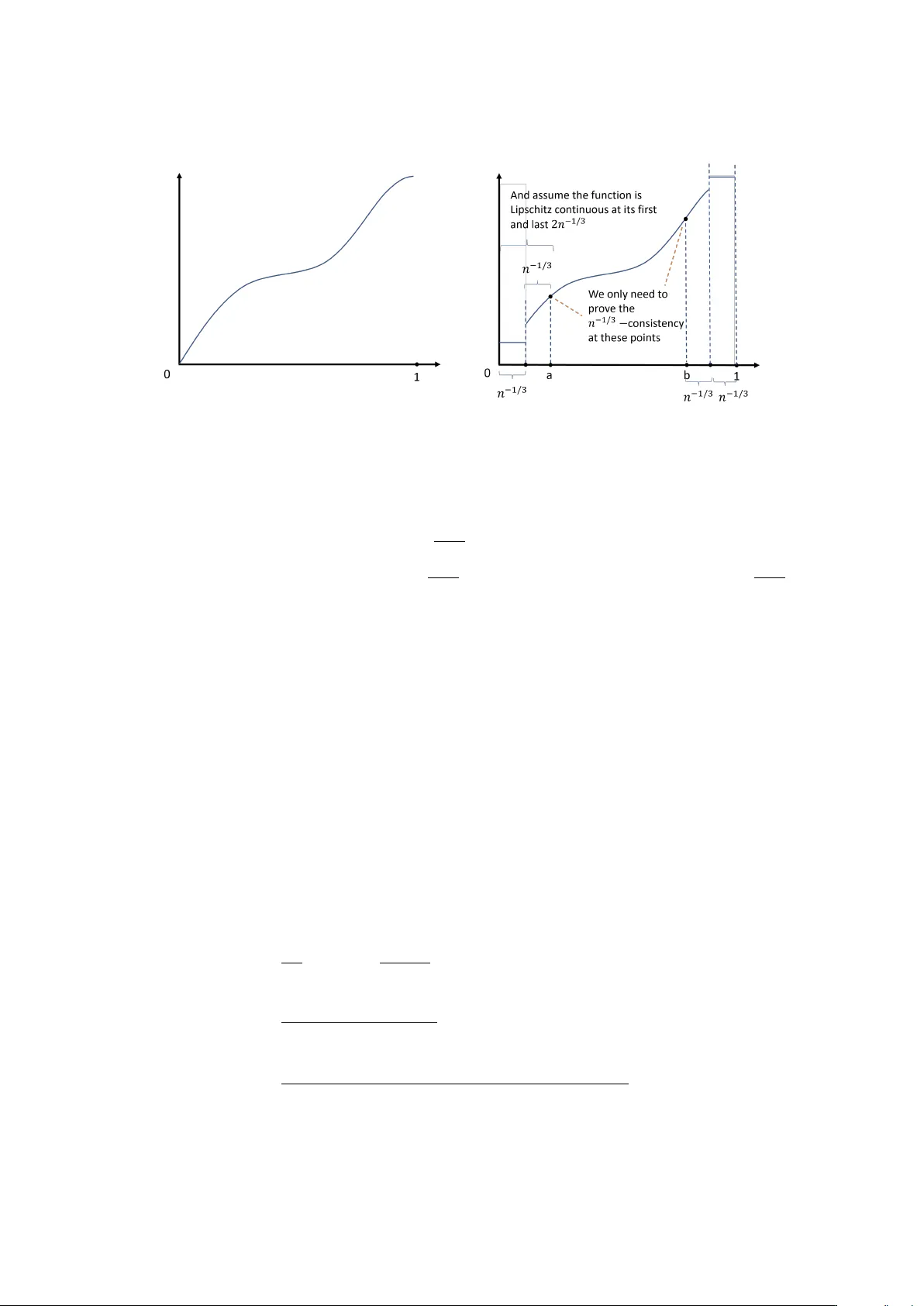
Isotonic prop ensit y score matc hing ∗ Mengshan Xu † and T aisuk e Otsu ‡ Jan uary 27, 2025 Abstract W e prop ose a one-to-many matching estimator of the av erage treatment effect based on prop ensit y scores estimated by isotonic regression. This approach is predicated on the assumption of monotonicit y in the propensity score function, a condition that can be justified in many economic applications. W e sho w that the nature of the isotonic estimator can help us to fix man y problems of existing matching metho ds, including efficiency , c hoice of the num b er of matc hes, choice of tuning parameters, robustness to propensity score missp ecification, and b ootstrap v alidity . As a b y-pro duct, a uniformly consisten t isotonic estimator is developed for our prop osed matching method. 1 In tro duction In b oth randomized exp erimen ts and observ ational studies, matching estimators are widely used to estimate treatment effects. This pap er prop oses a no vel one-to-man y prop ensit y score matc hing metho d of the av erage treatmen t effect (A TE), where the prop ensit y score is assumed to be monotone increasing in the exogenous co v ariate and is estimated b y the isotonic regression. Our matc hing scheme is exact, i.e., for the outcome Y , the binary treatment W , the cov ariate X , and a sample of size N , the matched set for the i -th unit is defined as J ( i ) = { j = 1 , . . . , N : W j = 1 − W i and ˜ p ( X j ) = ˜ p ( X i ) } , ∗ W e are grateful to Markus F r¨ olic h, Daniel Gutknec ht, Phillip Heiler, Lih ua Lei, Y oshi Rai, Christoph Rothe, Carsten T renkler, and participants at the econometrics seminar at Mannheim 2022, NASMES 2023, and IAAE 2023, for helpful comments and discussions. W e also would lik e to thank a co-editor and anon ymous referees for helpful commen ts to revise the paper. † Departmen t of Economics, Univ ersity of Mannheim, L7 3-5, 68161, Mannheim, German y . Email: mengshan.xu@uni-mannheim.de ‡ Departmen t of Economics, London School of Economics, Hough ton Street, London, WC2A 2AE, UK. Email: t.otsu@lse.ac.uk 1 where ˜ p ( · ) is a uniformly consisten t isotonic estimator of the prop ensit y score developed in Section 2.2. F or m ulti-dimensional co v ariates X , w e employ a monotone index mo del and consider the matched set: J ( i ) =  j = 1 , . . . , N : W j = 1 − W i and ˜ p ˜ α ( X ′ j ˜ α ) = ˜ p ˜ α ( X ′ i ˜ α )  , where ˜ p ˜ α ( · ) is a uniformly consistent monotone single-index estimator of the prop ensity score dev elop ed in Section 4. Remark ably , the isotonic estimator pro v es to b e esp ecially w ell-suited as the initial nonpara- metric estimator in a t wo-stage semiparametric ap proach to estimating the A TE. It incorporates features of b oth matching and weigh ting estimators into the second-stage A TE estimator, ad- dressing at least five issues commonly encountered b y existing matching metho ds in the causal inference literature. First, it is well kno wn that the existing matching estimators of the A TE with a fixed num b er of matc hes are inefficien t (Abadie and Im b ens, 2006) since they do not balance bias and v ariance in the second-stage estimation. In comparison, our isotonic matching estimator is more efficien t. In the univ ariate case, our metho d attains the semiparametric efficiency b ound; in the multi- v ariate case, where the efficiency b ound b ecomes more complicated, we show that our proposed estimator p erforms better than those based on a fixed n um b er of matc hes with prop ensit y scores deriv ed from widely used parametric mo dels suc h as probit and logit, which are prev alen t in applied research. Second, although the p erformance of fixed-n umber matc hing estimators can b e improv ed b y increasing the n umber of matches with the sample size, the efficiency gain is somewhat artificial (Im b ens, 2004) since the optimal num b er of matches and data-dep enden t w a ys of choosing it ha ve b een op en questions. How ever, these issues are addressed by recent pap ers by Armstrong and Koles´ ar (2021) and Lin et al. (2023). By sp ecifying a large enough Lipschitz constan t, Armstrong and Koles´ ar (2021) sho wed that the matching estimator with the num b er of matches set to one is minimax optimal if the conditional mean is restricted to b e Lipschitz; b y adding an estimated correction term. Lin et al. (2023) ga ve the optimal n umber of matches for a bias- corrected matching estimator. In this pap er, we argue that the isotonic estimator can provide an alternativ e solution: It gives a piece-wise monotone increasing estimator, whic h partitions observ ations in to differen t groups. Within these groups, the treated and untreated observ ations ha ve the same estimated prop ensity scores, so they can b e naturally matched to each other without the need of choosing the n umber of matches, weigh ts, and relev an t distance measures. 2 (F or our metho d, the distance is zero under an y measure.) In con trast, these c hoice problems are una voidable in traditi onal metho ds for both cov ariates matching and propensity score matc hing, no matter whether they are based on the in v erse v ariance matrix (e.g., Abadie and Im b ens, 2006) or the (empirical) density function (e.g., Im b ens, 2004) of co v ariates. Surprisingly , the set of the matc hing counterparts adaptively selected b y the isotonic estimator automatically b ecomes the optimal c hoice in the second stage, in that it ac hieves the semiparametric efficiency b ound of A TE (Hahn, 1998) for the univ ariate case. Third, compared to other semiparametric matching metho ds, where the first stage propensity score is estimated with kernel or series-based tec hniques, our metho d is more practical in a t wofold sense. It is not only free from the c hoice of the optimal n umber of matc hes, as men tioned in the second point abov e, but also do es not inv olv e smo othing parameters of con ven tional nonparametric metho ds, suc h as series length or bandwidth. In general, choosing the tuning parameters of a first-stage nonparametric estimator remains a difficult op en question in the semiparametric estimation literature. The MSE optimal tuning parameter is usually not a go od choice since the optimal first-stage estimator of the n uisance function do es not imply the optimalit y of the second-stage semiparametric estimation (Bick el and Rito v, 2003). T o ensure the √ N − consistency of a semiparametric estimator, “undersmo othed” tuning parameters should be applied (New ey , 1994). But it is difficult to find a clear standard for shrinking tuning parameters b elo w their MSE optimal v alues. The non-smo oth nature of the isotonic estimator, on the other hand, turns out to automatically render an adequate amount of undersmo othing. At the cost of a monotonicit y assumption imposed on the n uisance function, our proposed estimator av oids this choice problem while still main taining other desirable prop erties of a decent semiparametric estimator, such as √ N − consistency or efficiency . F ourth, compared to p opular parametric mo dels of prop ensit y scores, such as probit and logit, our proposed metho d con tains a nonparametric first stage, so it is more robust to mo del missp ecification. W e ackno wledge that combined with a single index structure, the probit and logit mo dels can also approximate many different data-generating pro cesses. But our metho d will alw ays be more robust than them since b oth probit and logistic functions are monotone increasing themselves. In other words, the isotonic regression can w ell estimate all the data generating pro cesses that can be well appro ximated by probit or logit model, but not vice versa. In addition, this robustness is achiev ed without costing the efficiency (compared to parametric metho ds) of the second-stage matc hing estimator. Fifth, it is well kno wn that the nonparametric b ootstrap of the fixed-num b er matching es- timator is inv alid in the presence of contin uous co v ariates (Abadie and Imbens, 2008). In the 3 past decade, muc h work has b een done to solv e this problem by prop osing clev erly structured wild b ootstrap procedures. Otsu and Rai (2017) prop osed a consistent wild b o otstrap for co- v ariates matc hing, and their approach w as extended by Bo dory et al. (2016) and Adusumilli (2020) to prop ensit y score matc hing estimators. In our pap er, we show that all these intricate b ootstraps are no longer necessary in the case of monotone increasing propensity scores since the nonparametric b o otstrap inference is asymptotically v alid for our isotonic matching estimator. Our metho d relies on the monotonicity assumption on prop ensit y scores. Monotonicit y is a natural shap e restriction that can b e justified in man y applications in so cial science, economic studies, and medical research. W ell-kno wn examples in economics include the demand function, whic h is usually monotone decreasing in prices, and the supply or the utility functions, which are often monotone increasing in quantities. F urthermore, many functions deriv ed from cumu- lativ e distribution functions (CDF) inherit the monotonicit y from the latter. F or example, in a threshold-crossing binary choice mo del Y =      1 if X ′ β 0 > ε 0 if X ′ β 0 ≤ ε , (1) the conditional exp ectation of Y on X can b e written as E [ Y | X ] = P ( Y = 1 | X ) = F ε ( X ′ β 0 ), where F ε ( · ) is the CDF of an indep enden t noise ε . If we assume ε ∼ N (0 , 1), (1) b ecomes a probit mo del; if we assume ε ∼ Logistic(0 , π 2 3 ), it b ecomes a logit mo del. Although b oth parametric mo dels are widely applied in estimating the probability of treatments, we can relax the distributional assumptions on ε and express (1) with a se miparametric mo del Y = F ε ( X ′ β 0 )+ ν , where F ε ( · ) is a nonparametric link function. W e emphasize that the link function is monotone increasing b y construction. See Cosslett (1983, 1987, 2007), Matzkin (1992), and Klein and Spady (1993) for more discussions of the mo del (1). 1 One of the main challenges of dev eloping the asymptotic properties of the proposed estimator is the inconsistency of the isotonic estimator at its b oundaries, sometimes called the “spiking” problem in the literature. If the dep enden t v ariable is binary , there is a non-trivial probabilit y for a non-shrinking group of left-end estimates to b e exactly zero ev en under the strict ov erlap condition, regardless of the sample size; the right-end estimates hav e a similar issue. As a result, the matched sets for observ ations at tw o ends are empty , and we cannot construct a 1 Although this paper explores monotonicity of the prop ensit y score function, our isotonic regression approac h ma y b e extended to the regression-based estimators with monotonicit y constraints on the exp ected outcome functions E [ Y (1) | X ] and E [ Y (0) | X ]. How ev er, it should be noted that if monotonicity is imp osed on the link functions of index mo dels, the regression-based approach is clearly more restrictiv e than the prop ensit y-score- based approac h (b ecause monotonicity on F ε ( · ) is not substantiv e). 4 v alid sample analog of A TE. F urthermore, observ ations near tw o ends are matc hed according to inconsistently estimated prop ensit y scores, which are biased tow ards zero or one, resulting in a detrimental effect on the A TE estimator similar to the one caused b y limited ov erlaps (Khan and T amer, 2010; Rothe, 2017; among others). Although truncating those observ ations, whose prop ensit y scores (either estimated parametrically or nonparametrically) are closer to 0 and 1, is widely implemen ted in applied work, this strategy has tw o ca veats if one w orks with the isotonic estimator. The first problem is the size of truncation: If to o little was truncated, it might b e insufficien t to correct the b oundary problem. A safe choice of truncation in the literature for differen t problems inv olving isotonic estimators is to truncate the first and last α N -th quan tile, with α N ∼ N − 1 / 3 (or up to a logarithmic factor, see W righ t, 1981; Durot, Kuliko v and Lopuha¨ a, 2013; and Babii and Kumar, 2021). How ev er, this truncation sc heme is to o muc h for our purpose. In fact, for an y α N suc h that α N N 1 / 2 → ∞ , the truncated A TE estimator migh t b e no longer √ N -consisten t. 2 Second, as discussed in App endix A.6.2, one of the k ey conditions for √ N - consistency and efficien t estimation of A TE is (58) b elo w, but whether this condition still holds after truncation is unclear. T o solve these tw o problems, we extend the everywhere-consisten t isotonic estimator of Meyer (2006) to a uniformly consistent isotonic (hereafter, UC-isotonic) estimator, which is b y design to suit our tw o-stage semiparametric matc hing estimator. The prop osed estimation pro cedure does not in volv e an y truncation, the abov e-men tioned fav orable prop erties of the isotonic estimator remain in tact, and the full set of data is utilized in b oth the first stage estimation of the prop ensit y score and the second stage estimation of A TE. Our prop osed metho d builds on the large literature of causal inference for cov ariate and prop ensit y score matching estimators, e.g., Rosen baum and Rubin (1983, 1984), Rosen baum (1989), Hec kman, Ic himura and T o dd (1997, 1998), Hec kman, Ic himura, Smith and T o dd (1998), Dehejia and W ah ba (1999), Abadie and Imbens (2006, 2008, 2011, 2016), Imbens (2004), F r¨ olic h (2004), F r¨ olich, Huber and Wiesenfarth (2017), Otsu and Rai (2017), Bo dory , Camp ono vo, Hub er and Lec hner (2016), Adusumilli (2020), among others. The prop ensit y score matc hing estimators studied in the literature mainly use parametrically estimated prop ensity scores, suc h as probit and logit. Our prop osed metho d, in con trast, uses a sp ecial type of nonparametric estimator, the isotonic estimator, to estimate the prop ensit y score. The isotonic estimator has a long history . The earlier w ork includes Ay er et al. (1955), Grenander (1956), Rao (1969, 1970), and Barlo w and Brunk (1972), among others. The isotonic 2 This problem is not univ ersal for ev ery semiparametric estimator. F or example, for a partially linear mo del Y = X β + ψ ( Z ) + ε , w e can truncate more than its N − 1 / 2 -th quan tile, and the estimator of β main tains √ N - consistency . In fact, one can get √ N -rates ev en if β is estimated from an arbitrary sub-sample with a size prop ortional to N since different X ’s are linked to the same β . How ever, for A TE, in general, the truncated parts directly constitute estimation bias. 5 estimator of a regression function can b e form ulated as a least square estimation with a mono- tonicit y constraint. Suppose that the conditional exp ectation E [ Y | X ] = p 0 ( X ) is monotone increasing. Then, for an iid random sample { Y i , X i } N i =1 , the isotonic estimator is the minimizer of the sum of squared errors, min p ∈M P N i =1 { Y i − p ( X i ) } 2 , where M is the class of monotone increasing functions. The minimizer can be calculated with the p o ol adjacent violators algo- rithm (Barlow and Brunk, 1972), or equiv alen tly b y solving the greatest con vex minorant of the cum ulative sum diagram { (0 , 0) , ( i, P i j =1 Y j ) , i = 1 , . . . , N } , where the corresp onding { X i } N i =1 are ordered sequence. See Gro eneb oom and Jongbloed (2014) for a comprehensiv e discussion of differen t aspects of isotonic regression. Our work is link ed to the v ast literature on semiparametric estimation, e.g., Cham b erlain (1987), Robinson (1988), New ey (1990, 1994), v an der V aart (1991), Andrews (1994), Hahn (1998), Ai and Chen (2003), Bic kel and Ritov (2003), Chen, Linton and V an Keilegom (2003), Chen and San tos (2018), among others. In most of the w orks cited ab o ve, nonparametric metho ds inv olving smo othing parameters w ere applied at the initial stage, while our work uses the isotonic estimation that is non-smo oth and do es not in volv e smo othing parameters. On the other hand, the double machine learning estimators (hereafter, DML; see, e.g., Robins, Rotnitzky and Zhao, 1995; Chernozh uko v et al ., 2017, 2018; among others) provide efficient estimators of the A TE that do not rely on sub jectiv e c hoices of smo othing parameters, thereby , to some extent, sharing man y adv an tages of our approach. W e provide a detailed comparison b et w een the isotonic propensity score matching estimator and the DML for the A TE in Section 3.4. There are some authors working on concrete semiparametric models with plug-in isotonic estimators. Huang (2002) studied the prop erties of the monotone partially linear mo del, and his w ork w as extended b y Cheng (2009) and Y u (2014) to the monotone additive mo del. Balabdaoui, Durot and Jank owski (2019) studied the monotone single index model with the monotone least square metho d, and Gro eneb oom and Hendrickx (2018), Balab daoui, Gro eneb o om and Hen- dric kx (2019), and Balab daoui and Groeneb o om (2021) (the last t wo pap ers are called BGH hereafter) dev elop ed a score-t yp e approac h for the monotone single index mo del and show the single index parameter can b e estimated at √ N -rate. Building on previous w orks, Xu (2021) studied a general framework of semiparametric Z-estimation with plug-in isotonic estimators, monotone single-index estimators, or monotone additive estimators, and applied the generic re- sult to in v erse probabilit y w eigh ting (IPW) estimators of A TE. F or the augmen ted IPW (AIPW) mo del, Qin et al. (2019) and Y uan, Yin and T an (2021) applied the monotone single index mo del to estimate the prop ensit y score, then plugged the estimated prop ensit y scores with other esti- 6 mates of p otential outcomes in to a doubly-robust momen t function. Their asymptotic results rely on the consistent estimations of b oth prop ensit y scores and p oten tial outcomes, and thus differ from our approac h. In terms of applying isotonic regression to estimate the A TE, the primary difference b et ween this pap er and Chapter 3 of Xu (2021) is that w e address the b oundary issue inheren t in the isotonic estimator, while Xu (2021) relies on a stronger assumption adapted from Assumption 5.1 in New ey (1994). In the pro cess of writing this paper, w e hav e gradually realized that this assumption do es not automatically apply to the IPW estimator, although it straigh tforwardly holds for some other semiparametric mo dels, suc h as the monotone partially linear mo del and the monotone single index mo del, wherein the plugged-in isotonic estimator is not in the de- nominator. Compared to Chapter 3 of Xu (2021), the main contributions of this pap er are: (i) prop osing a UC-isotonic estimator that is suitable as the first-stage estimator in a prop en- sit y score matching estimator of the A TE; (ii) rev ealing the equiv alence b et w een the matching estimator and the IPW estimator when the first-stage prop ensit y score is e stimated via UC- isotonic regression; and (iii) based on this equiv alence, enric hing the literature on prop ensit y score matching by in tro ducing a new approac h that addresses several problems of the existing matc hing methods, as detailed at the b eginning of this introduction. 3 The rest of the pap er is organized as follo ws. After in tro ducing the setting and notations, Section 2 shows the implemen tation and asymptotic properties of the prop osed isotonic matc hing estimator with a univ ariate cov ariate. Section 3 compares our approac h with existing matching estimators as w ell as the double machine learning estimator for the A TE. The univ ariate results are extended to the case of m ultiv ariate co v ariates in Section 4, where the prop ensit y score is mo deled b y a semiparametric single-index mo del with an unknown monotone increasing link function. In Section 5, we establish the v alidity of the nonparametric b ootstrap. Mon te-Carlo sim ulation studies are presen ted in Section 6. All proofs are presen ted in App endix, while addi- tional theoretical details and simulation comparisons are provided in Supplemen tary Material. 3 A t almost the same time, an indep enden t work b y Liu and Qin (2022) deriv ed a similar equiv alence result for the a verage treatment effect on treated (A TT). Recently , a revised v ersion of Liu and Qin (2022) is published as Liu and Qin (2024). There are t wo main differences betw een our paper and their pap ers. First, we formally address the b oundary problem of the isotonic estimator and achiev e the √ N -normality of the A TE estimator b y prop osing a uniformly consisten t isotonic estimator. Second, our asymptotic analysis of the mo del with m ultiv ariate co v ariates in Section 4 fo cuses on a more general case, where the influence of the estimation errors from the parametric comp onent of the first-stage monotone single index mo del is main tained. 7 2 Main results 2.1 Setup and isotonic prop ensity score Supp ose we observe the triple ( Y , W , X ) dra wn randomly from the pro duct space Z = R ×{ 0 , 1 } × X . Within the triple, W ∈ { 0 , 1 } is a binary treatmen t v ariable, Y = W · Y (1) + (1 − W ) · Y (0) is an outcome v ariable with p oten tial outcomes Y (1) and Y (0) for W = 1 and 0, resp ectiv ely , and X is a scalar co v ariate with contin uous domain X = [ x L , x U ] ⊂ R . In this section, we ten tatively assume X is scalar, and discuss extensions for multiv ariate X in Section 4. Without loss of generality , { Y i , W i , X i } N i =1 is an iid sample of ( Y , W , X ) and is ordered by X . If X is con tinuously distributed, we should hav e X 1 < X 2 < · · · < X N with probability one (i.e., no ties). In this section, we consider the estimation of the A TE, τ = E [ Y (1) − Y (0)], b y matching the prop ensit y score p ( x ) = P ( W = 1 | X = x ) = E [ W | X = x ], where p ( · ) is an unkno wn monotone increasing function. In particular, w e estimate p ( · ) by the isotonic estimator ˆ p ( · ) = arg min p ∈M N X i =1 { W i − p ( X i ) } 2 , (2) where M is the class of all monotone increasing functions defined on X . Since Brunk (1958), this isotonic regression estimator has b een extensively studied in the statistics literature (see, e.g., Barlo w et al. , 1972, and Gro eneb oom and Jongblo ed, 2014, for an ov erview). One of the w ell-known features of isotonic regression is that the estimator ˆ p ( · ) is a monotone increasing piecewise constant function with jump p oin ts at { X n k } K k =1 for some in teger K with 1 ≤ K ≤ N . By these jump points, the sample is divided in to K disjoin t groups, with { n k } K k =1 denoting the first indices of these K groups. F urther, we let N k denote the n um b er of observ ations b elonging to the k -th group. Based on these definitions, it holds that n k + N k = n k +1 for each k = 1 , . . . , K − 1, and P K k =1 N k = N . Note that the integer K and the corresp onding disjoin t groups are automatically determined by the isotonic estimation algorithm (see the form ula (7) b elo w), rather than b eing c hosen by the user. T o av oid ambiguit y caused b y splitting a flat piece into sev eral sub-pieces with the same estimated v alue, w e imp ose ˆ p ( X n 1 ) < ˆ p ( X n 2 ) < · · · < ˆ p ( X n K ) , (3) to ensure uniqueness of this partition (i.e., if ˆ p ( X n k ) = ˆ p ( X n k +1 ), w e simply com bine the groups 8 k and k + 1). Then, the isotonic estimator ˆ p ( · ) is c haracterized as follo ws. Assumption 1. [Sampling] { Y i , W i , X i } N i =1 is an indep endent and identic al ly distribute d (iid) sample of ( Y , W, X ) ∈ R × { 0 , 1 } × X , wher e X = [ x L , x U ] ∈ R . X is c ontinuously distribute d, and the sample { Y i , W i , X i } N i =1 is indexe d ac c or ding to X 1 < X 2 < · · · < X N . Prop osition 1. Under Assumption 1, the isotonic estimator ˆ p ( · ) satisfying (3) p artitions the sample into K disjoint gr oups in the sense that for e ach k = 1 , . . . , K and i = n k , . . . , n k + N k − 1 , ˆ p ( X i ) = 1 N k n k + N k − 1 X j = n k W j . (4) T o define our prop ensit y score matc hing estimator based on ˆ p ( · ), let N k, 1 and N k, 0 denote the num b ers of treated and controlled observ ations within group k , i.e., N k, 1 = P n k + N k − 1 i = n k W i and N k, 0 = N k − N k, 1 . Our one-to-man y matching metho d is implemen ted within each of these K groups, and each treated (controlled) observ ation in group k will b e matched with its N k, 0 ( N k, 1 ) counterparts, whic h b elong to the same group and ha ve the same v alue of the estimated prop ensit y score. The following results directly follow from Prop osition 1. Prop osition 2. Supp ose Assumption 1 holds. (i) [Isotonic estimator] F or e ach inte ger k = 1 , . . . , K , the isotonic estimator ˆ p ( · ) for p ( · ) is r epr esente d as ˆ p ( x ) = N k, 1 N k , (5) for e ach x ∈ { X i } n k + N k − 1 i = n k . (ii) [Existenc e of matching c ounterp arts] F or any i ∈ { 1 , . . . , N } with 0 < ˆ p ( X i ) < 1 , the set of its matching c ounterp arts { j : W j = 1 − W i , ˆ p ( X j ) = ˆ p ( X i ) } is non-empty. Before we pro ceed, w e need to solv e the problem of the p oten tial lack of matc hing coun- terparts for those i ’s with ˆ p ( X i ) = 0 or 1. Under the strict ov erlaps (in Assumption 3 b elo w), the problem is essen tially asso ciated with the inconsistency of the isotonic estimator at the b oundary . In the next subsection, we prop ose a mo dified isotonic estimator that is uniformly consisten t on X . 2.2 Uniformly consisten t isotonic estimator Lik e other nonparametric estimators, the isotonic estimator is imprecise at the b oundary . If w e apply the isotonic estimator to the binary dep enden t v ariable W , there is a non-trivial 9 probabilit y of ˆ p ( X i ) = 0 or 1 ev en if the true prop ensit y score p ( x ) is b ounded a wa y from zero and one for all x ∈ X . F or example, if ˆ p ( X 1 ) = 0, (5) implies N 1 , 1 = 0, i.e., there are no matc hing coun terparts for the treated units. T o fix this problem, we prop ose a mo dified isotonic estimator that is uniformly consisten t in its domain at a (log N ) 1 / 3 N − 1 / 3 rate and is easy to implement. F or the sample { W i , X i } N i =1 with X 1 < · · · < X N , we transform { W i } N i =1 in to { ˜ W i } N i =1 b y av eraging its first and last ⌊ N 2 / 3 ⌋ observ ations: ˜ W i =              1 ⌊ N 2 / 3 ⌋ P ⌊ N 2 / 3 ⌋ i =1 W i for i ≤ ⌊ N 2 / 3 ⌋ W i for ⌊ N 2 / 3 ⌋ < i ≤ N − ⌊ N 2 / 3 ⌋ 1 ⌊ N 2 / 3 ⌋ P N i = N −⌊ N 2 / 3 ⌋ +1 W i for i > N − ⌊ N 2 / 3 ⌋ . (6) Our prop osed UC-isotonic estimator is obtained b y implemen ting the standard isotonic regres- sion of ˜ W on X : ˜ p ( x ) =              max s ≤ i min t ≥ i P t j = s ˜ W j / ( t − s + 1) for x = X i ˜ p ( X i ) for X i − 1 < x ≤ X i ˜ p ( X N ) for x > X N . (7) A similarly mo dified estimator w as proposed b y Mey er (2006), where she av eraged the first and last ⌈ log( N ) ⌉ dependent v ariables instead of the first and last ⌊ N 2 / 3 ⌋ ones. The c hoices are different because she fo cuses on the consistency of the isotonic estimator itself, while we are in terested in the p erformance of the second-stage matching estimator. T o achiev e an N − 1 / 2 rate at the second stage, we need the isotonic estimator to b e uniformly consistent at a rate faster than N − 1 / 4 , which won’t b e achiev ed under Mey er’s c hoice. Meyer (2006) presented a theorem regarding the consistency of the mo dified estimator at the b oundary; ho wev er, a proof of consistency was not provided, nor w as the rate of conv ergence discussed. In this pap er, we formally establish the uniform con vergence rate of the mo dified isotonic estimator ˜ p ( · ). T o this end, w e impose the following assumption. Assumption 2. [Monotonicity and c ontinuity] (i) p ( x ) = E [ W | X = x ] is a monotone incr e asing function of x ∈ X , (ii) p ( x ) is c ontinuously differ entiable with its first derivative p (1) ( x ) > 0 for al l x ∈ X , and (iii) X has a c ontinuous density f ( x ) satisfying that for some p ositive c onstants f and f , it holds f < f ( x ) < f al l x ∈ X . Assumption 2 (i) is our main assumption, the monotonicity of p ( · ). Assumption 2 (ii) is re- 10 quired for the √ N − consistency of the second-stage matching estimator. The same assumption has b een adopted by Gro enebo om and Hendric kx (2018; Assumption A2) and by BGH (As- sumption A3 and its accompan ying remark; see also Lemma 22 in the supplemen tary material of BGH) in the con text of the monotone single index mo del. If we believe that the underlying prop ensit y score function has some flat parts where p (1) ( x ) = 0, we could first run an isotonic estimation of ˜ W i + c · X i on X i , where c is a p ositiv e constan t, to obtain ˜ p c ( x ). Then, by sub- tracting the linear trend c · x from ˜ p c ( x ), w e obtain a consistent estimator of p ( x ). 4 Assumption 2 (iii) imp oses an upper and low er bound for the density of X . T o av oid unnecessarily rep eatedly defined notations, we let the same set of notations, K, N k, 1 , N k , and n k , denote the n umber of groups, the num b er of treated observ ations in group k , the n umber of members in group k , and the index of the first element of group k , under the grouping scheme giv en by the UC-isotonic estimator ˜ p ( · ) ( N k, 1 is calculated with the original treatmen t v ariable { W i } N i =1 ). W e obtain an analogous result to Proposition 2 for the UC-isotonic estimator. Prop osition 3. Under Assumptions 1 and 2, it holds (i) N 1 ≥ ⌊ N 2 / 3 ⌋ and N K ≥ ⌊ N 2 / 3 ⌋ . (ii) ˜ p ( x ) = N k, 1 N k for e ach k = 1 , . . . , K and x ∈ { X i } n k + N k − 1 i = n k . (iii) N 1 = O p ( N 2 / 3 ) and N K = O p ( N 2 / 3 ) . P art (i) of this proposition says that all the av eraged W i ’s at the b eginning and end of the data are absorbed in the first and the last group. Part (ii) pro vides an analogous representation of the UC-isotonic estimator ˜ p ( · ) as ˆ p ( · ). While Part (i) giv es a low er b ound of the sizes of the first and the last group, Part (iii) gives (sto c hastic) upp er b ounds of them. Based on this prop osition, the uniform conv ergence rate of the UC-isotonic estimator is obtained as follows. Theorem 1. Under Assumptions 1 and 2, it holds sup x ∈X | ˜ p ( x ) − p ( x ) | = O p  log N N  1 / 3 . Finally , to guaran tee the existence of matching counterparts by ˜ p ( · ), we imp ose the strict o verlap condition. 4 T echnically , if p ( · ) has some flat parts where p (1) ( x ) = 0, then the original estimator ˜ p ( · ) may not satisfy the requiremen t in (50) in Appendix A.6, | δ ( x ) − ¯ δ N ( x ) |≤ C 0 | p ( x ) − ˜ p ( x ) | . Flat parts in p ( · ) imply that p ( x ) − ˜ p ( x ) = 0 migh t hold within an entire interv al, p otentially leading to a violation of (50). In contrast, if p ( · ) is strictly monotone increasing, then p ( · ) and ˜ p ( · ) will cross at most once within eac h partition given b y the isotonic estimator, since ˜ p ( · ) is a piecewise flat function. W e refer to Sections 10.2-10.3 and Figure 10.1 of Gro enebo om and Jongbloed (2014) for more details. 11 Assumption 3. [Strict overlaps] Ther e exist p ositive c onstants p and ¯ p such that 0 < p ≤ p ( x ) ≤ ¯ p < 1 for al l x ∈ X . Assumption 3 is standard in the treatment effect literature. It is necessary for the identifica- tion and √ N -consisten t estimation of the A TE. Com bining Prop osition 3 and Theorem 1 with Assumption 3, the existence of the matc hing counterparts b y ˜ p ( · ) is obtained as follows. Corollary 1. Supp ose Assumptions 1-3 hold. F or e ach i = 1 , . . . , N , the set of its match- ing c ounterp arts { j = 1 , . . . , N : W j = 1 − W i , ˜ p ( x j ) = ˜ p ( x i ) } is non-empty with pr ob ability appr o aching one. 2.3 Isotonic prop ensit y score matc hing Based on the UC-isotonic estimator ˜ p ( · ), the isotonic prop ensit y score matching estimator for the A TE τ can b e implemen ted as follo ws. 1. T ransform the sample { Y i , W i , X i } N i =1 indexed by X 1 < · · · < X N in to { Y i , ˜ W i , X i } N i =1 using (6). 2. Compute the UC-isotonic estimator ˜ p ( · ) using (7). 3. F or eac h i = 1 , . . . , N , compute the matching coun terparts J ( i ) = { j = 1 , . . . , N : W j = 1 − W i and ˜ p ( X j ) = ˜ p ( X i ) } . (8) 4. Calculate the matching estimator for the A TE τ by ˆ τ = 1 N N X i =1 (2 W i − 1)   Y i − 1 M i X j ∈J ( i ) Y j   , (9) where M i = |J ( i ) | is the n umber of matc hes for i . W e pro ceed with the follo wing assumptions. Assumption 4. [Data gener ating pr o c ess] (i) E [ Y (0) 2 ] < ∞ and E [ Y (1) 2 ] < ∞ , (ii) E [ Y (0) | X = x ] and E [ Y (1) | X = x ] ar e c ontinuously differ entiable for al l x ∈ X , (iii) for D ( Z ) = W Y p ( X ) 2 + Y (1 − W ) { 1 − p ( X ) } 2 , ther e exist p ositive c onstants c 0 and M 0 such that E [ | D ( Z ) | m | X = x ] ≤ m ! M m − 2 0 c 0 holds for al l inte gers m ≥ 2 and every x , and (iv) Y (1) , Y (0) ⊥ W | X almost sur ely. Assumption 4 (i)-(iii) regulates the tail b eha viors of the (conditional functions of ) p oten tial outcomes, which are necessary for √ N -consisten t estimation. Assumption 4 (iv) is the standard 12 unconfoundedness assumption. Under these assumptions, we hav e the following k ey equiv alence result. Theorem 2. Under Assumptions 1-4, the matching estimator ˆ τ for the A TE τ using the UC- isotonic estimator ˜ p ( · ) is e qual to the c orr esp onding inverse pr ob ability weighting (IPW) estima- tor. Remark on Theorem 2 Im b ens (2004) p ointed out that with M → ∞ and M /N → 0, the matching estimator is essen tially like a regression estimator. In comparison, w e find out that with prop ensit y scores estimated by the UC-isotonic estimator, the (prop ensit y score) matc hing estimator is n umerically equal to the weigh ting estimator in each finite sample. This equiv alence is tigh tly asso ciated with the fact that th e isotonic estimator can b e regarded as a t yp e of partitioning estimator (e.g., Gy¨ orfi et al. , 2002; Cattaneo and F arrell, 2013). See Section 3.1 below for a further comparison of isotonic and partitioning estimators within the con text of a tw o-stage matching estimator of the A TE. Additionally , our metho d is related to the prop ensity score methods of blo c king, stratification, and radius matching (Rosenbaum and Rubin, 1983, 1985; Dehejia and W ahba, 1999, 2002; among others). See Section 3.2 for a comparison with these metho ds. Moreo ver, as mentioned in the in tro duction, the equiv alence result in Theorem 2 relies cru- cially on the implementation of the UC-isotonic estimator (7), whic h guaran tees that b oth the matc hing and IPW estimators at the second stage are w ell-defined. W e notice that the threshold ⌊ N 2 / 3 ⌋ in the algorithm (6) can b e in terpreted as an implicit tuning parameter. W e would like to p oint out that, first, it is conv enient to c ho ose since it dep ends only on the sample size N ; second, it is aimed at correcting the b oundary problem, whic h is also faced b y other semiparametric and ev en parametric matc hing methods. In practice, trimming estimated propensity scores is widely adopted, and the amount of trimming is chosen sub jectively in most cases. Our prop osed metho d provides transparent guidance for correcting this common boundary issue. F urthermore, to inv estigate the impact of different threshold c hoices, we ha ve included b oth theoretical analysis and simulation evidence in Sections S2 and S3.3 of the supplemen tary material, respe ctiv ely . Our main result, consistency and asymptotic normality of the isotonic prop ensit y score matc hing estimator, is obtained as follo ws. 13 Theorem 3. Under Assumptions 1-4, it holds ˆ τ p → τ and √ N ( ˆ τ − τ ) d → N (0 , Ω) , wher e Ω = V ( E [ Y (1) − Y (0) | X ]) + E [ V ( Y (1) | X ) /p ( X )] + E [ V ( Y (0) | X ) / (1 − p ( X ))] . W e note that the asymptotic v ariance Ω is the semiparametric efficiency bound for τ (see e.g., Hahn, 1998, and Hirano, Imbens and Ridder, 2003). Although w e ma y conduct inference based on an estimator of Ω, we suggest a b o otstrap inference metho d, whic h will b e discussed in Section 5. 3 Comparison to related prop ensit y score metho ds In this section, w e dra w comparisons of our approach with a range of related estimators for the A TE. The comparison with matc hing metho ds based on prop ensit y score estimated by partitioning estimator is presen ted in Section 3.1, the comparison with prop ensit y score methods of blocking, stratification, and radius matching is presen ted in Section 3.2, the comparison with matc hing metho ds based on prop ensit y score estimated by regression trees is presented in Section 3.3, and the comparison with the double machine learning (DML) estimator for the A TE can b e found in Section 3.4. 3.1 Prop ensit y score estimated by partitioning estimator One notable feature of the prop osed isotonic prop ensit y score matc hing metho d is that it is a one-to-many matching metho d that pro vides exact matc hes, as illustrated b y the formula (8). This is attributed to the isotonic estimator being considered a sp ecial t yp e of partitioning estimator, in which the v olume sizes of partitions are automatically chosen by the monotonicit y constrain t, and a simple av erage is implemen ted within each partition. The partitioning estimator is a nonparametric metho d for estimating regression functions. 5 It divides the domain of the running v ariables into disjoint partitions. Within eac h partition, a lo cal estimator is implemented b y the user, such as the sample mean, a linear estimator, or a series estimator. Eac h sample p oin t is exclusiv ely used in the estimation within the partition to whic h it b elongs. This feature simplifies the complex correlation structure of a matching estimator such that it achiev es equiv alence with an IPW estimator. F or the UC-isotonic estima- tor, this e quiv alence is presen ted by equation (42) in App endix A.5. In the resulting matching 5 W e refer to Gy¨ orfi et al. (2002) and Cattaneo and F arrell (2013) for comprehensive discussions of the partitioning estimator. 14 estimator of A TE, the same set of partitions serv es b oth the first- and the second-stage non- parametric estimation. Usually , these t wo stages are not asso ciated with each other since they ha ve distinct ob jects, the prop ensit y score and the p oten tial outcomes. Certainly , a matching estimator of the A TE that utilizes prop ensity scores estimated with a partitioning estimator should exhibit a similar equiv alence to the weigh ting estimator. How ever, the selection of the n umber of partitions and their sizes necessitates careful consideration, as they must meet sp e- cific undersmo othing conditions to secure the desired asymptotic properties of the second-stage A TE estimator. The challenge of selecting an appropriate undersmo othed bandwidth or volume size, as men tioned in the introduction, remains a difficult open question in the semiparametric estimation. In con trast, our prop osed isotonic matc hing estimator automatically c ho oses these tuning parameters, leading to the efficien t estimation of the A TE, as demonstrated in Theorem 3. 3.2 Prop ensit y score metho ds of blocking, stratification, and radius matc hing Our proposed isotonic matc hing estimator is also related to some of the seminal ideas in tro duced at the outset of the prop ensit y score metho ds: blo c king, stratification (Rosenbaum and Rubin, 1983; Dehejia and W ah ba, 1999, 2002), and radius matc hing (Rosenbaum and Rubin, 1985). The isotonic prop ensit y score matc hing shares similarities with blo cking and stratification matc hing on prop ensit y scores, notably: (i) they initially categorize data p oin ts in to distinct groups (or strata, blo c ks, partitions) according to estimated prop ensit y scores, and (ii) within eac h group, they calculate the conditional av erage treatment effect as the simple difference in means of outcomes betw een the treatmen t and comparison groups. The primary distinction lies in the grouping mechanism: for isotonic propensity score matching, the groups are determined adaptiv ely in a data-driven manner through isotonic regression, whereas for the stratification estimator of the A TE, the strata must b e explicitly sp ecified by the user. Another distinction is that for the isotonic prop ensit y score matching metho d, the same set of partitions is utilized for b oth the first and second stages of nonparametric estimation. As presented by Theorem 2, this c haracteristic leads to the equiv alence b et w een the matc hing and IPW estimator, result- ing in the efficient estimation of the A TE. In contrast, in the case of blo c king or stratification matc hing metho ds, particularly when the prop ensit y score is estimated using parametric mod- els, this equiv alence cannot generally b e established, and efficiency cannot b e assured without implemen ting some bias correction metho d. The case for the radius matching estimator is similar to the stratified matching estimator. The difference is that for stratified matc hing, each unit is matched solely with units from the 15 opp osite treatment group within the same stratum, while radius matching allows each unit to b e matc hed to several lo cal balls, the centers of which b elong to the opp osite treatmen t group. F or both radius and stratified matc hing es timators, the sizes of strata or the radii act as tuning parameters, which must b e chosen by the users when the prop ensit y score is estimated via parametric or nonparametric methods dep enden t on smoothing parameters (suc h as kernel or series estimation). These smoothing parameters pla y a key role in balancing the bias and v ariance, thereby significan tly affecting the second-stage estimator of A TE. In con trast, isotonic regression distinguishes itself b y automatically generating these partitions through the application of the monotonicit y constraint. 3.3 Prop ensit y score estimated by regression trees As metho ds of estimating the prop ensit y scores, the isotonic estimator and regression trees share sev eral similarities. First, b oth are nonparametric estimators that do not imp ose re- strictiv e parametric structures on the underlying resp onse function. Second, b oth approaches partition the domain of running v ariables (the feature space in regression tree terminology) in to several regions and use the sample a verage within each region as estimators. As a result, b oth estimators tak e the form of piecewise-constant functions. Third, both methods form their piecewise-constan t functions in data-adaptive manners. In particular, the partitions created by b oth metho ds dep end on the dep enden t v ariable (the response), which differentiates them from regular nonparametric metho ds, such as the kernel estimator. On the other hand, there are notable distinctions b et ween the tw o metho ds. First, b oth approac hes construct their piecewise-constan t functions differently: the partitions in a regression tree are obtained in a stepwise manner. In eac h step, a partition is chosen to ac hieve the maxim um marginal reduction of the mean square error (MSE), without imp osing any shap e constrain ts during this process. In con trast, the isotonic estimator employs a one-step approac h that determines partitions to minimize the MSE ov er the class of monotone functions. Second, although b oth approaches are data-driven, the isotonic estimator is free of smo othing parameters, whereas the regression tree dep ends on the user to sp ecify the tree’s length. (When the tree length is determined b y cross-v alidation, the user m ust select the p enalt y parameter.) Third, the regression tree is inheren tly designed for multi-dimensional problems, whereas the canonical form of isotonic regression addresses one-dimensional issues, given that the traditional definition of monotonicit y characterizes the relationship b et ween tw o v ariables. Nevertheless, the isotonic estimation can b e extended to m ultiv ariate cases b y b eing incorp orated into a partially linear mo del or a monotone single index mo del. The latter is illustrated in Section 4 b elo w. 16 T o summarize, the isotonic estimator necessitates the monotonicit y assumption in the under- lying resp onse function, a requiremen t not shared b y regression trees. This assumption, ho w ever, enables the isotonic estimation algorithm to automatically regulate the trade-off b et ween bias and v ariance. Conv ersely , when using regression trees, practitioners are task ed with the c hal- lenge of selecting an appropriate tree length to effectiv ely manage the balance b et ween bias and the risk of ov erfitting. The strength of regression trees is their natural aptitude for tackling m ultiv ariate problems. When emplo ying regression trees in the preliminary stage of prop ensit y score estimation as part of a t wo-stage approach to estimating the A TE, it is commonly com- bined with metho ds for bias correction and sample splitting, as discussed by Chernozh uko v et al. (2018). See Section 3.4 b elo w for more details ab out the comparison of our approach with the double machine learning estimator. 3.4 Double mac hine learning estimator The isotonic prop ensit y score matc hing estimator and the DML estimator for the A TE b oth share the b enefit of not requiring sub jectiv e choices of tuning parameters. F or estimating the A TE, a typical example of a DML estimator is giv en b y applying the sample splitting to the augmen ted inv erse probabilit y weigh ting (AIPW) estimator. In the following, we abstract from sample splitting to simplify notation: 1 N N X i =1 { ˆ ψ 1 ( X i ) − ˆ ψ 0 ( X i ) } + 1 N N X i =1 " W i ( Y i − ˆ ψ 1 ( X i )) ˆ p ( X i ) − (1 − W i )( Y i − ˆ ψ 0 ( X i )) 1 − ˆ p ( X i ) # = 1 N N X i =1  Y i W i ˆ p ( X i ) − Y i (1 − W i ) 1 − ˆ p ( X i )  − 1 N N X i =1  W i − ˆ p ( X i ) ˆ p ( X i ) ˆ ψ 1 ( X i ) − W i − ˆ p ( X i ) 1 − ˆ p ( X i ) ˆ ψ 0 ( X i )  , (10) where ˆ ψ 1 ( · ) and ˆ ψ 0 ( · ) are estimators of E [ Y (1) | X = · ] and E [ Y (0) | X = · ], resp ectively . The first and second lines of (10) presen t tw o formulations of the DML estimator for the A TE. The first terms in b oth lines correspond to the standard regression and IPW estimators, resp ectively , while the subsequent terms represent their bias-correction comp onen ts. The AIPW has been extensiv ely studied since the seminal work of Robins, Rotnitzky and Zhao (1995), Robins and Rotnitzky (1995); see also Newey , Hsieh, and Robins (1998, 2004), Sc harfstein, Rotnitzky and Robins (1999), Rothe and Firp o (2019), among others. In an in- fluen tial work, Chernozh uko v et al . (2018) combined orthogonal moment functions – of which the form ula (10) is a specific case for the A TE – with sample splitting, accommodating a broad arra y of the first-stage machine learners that are prone to bias due to regularization or mo del selection. Recen t developmen ts by Chernozh uk ov et al. (2022) and Chernozhuk o v, Newey and 17 Singh (2022) hav e prop osed metho ds for constructing the correction term without requiring an explicit function form for the bias correction. Both estimators hav e their o wn adv antages and comparativ e strengths. F rom a practical standp oin t, the isotonic propensity score matching metho d stands out for its simplicit y and ease of implementation: it do es not require the correction terms, thereby sparing the effort of estimating the conditional means of p oten tial outcomes and sidesteps the c hallenges asso ciated with their correct sp ecification. In contrast, the DML estimator’s efficiency relies on correctly sp ecifying and effectiv ely estimating b oth the prop ensit y score and the conditional means of p oten tial outcomes. A misstep in either leads to a consistent y et inefficient estimator. On the other hand, the DML estimator exhibits great flexibility: through the use of sample splitting, it supp orts a v ariety of first-stage estimators, accommo dating high dimensional data or highly complex function classes, such as random forest, neural netw orks, and other adv anced mac hine learning technologies. F rom a technical standp oin t, the isotonic prop ensity score matching and the DML for the A TE represen t tw o distinct pathw a ys of semiparametric estimation: undersmo othing and bias correction. Both strategies aim for √ N -consisten t (or efficient in certain cases) estimators (see New ey , 1994, for a relev an t discussion). The undersmo othing strategy dep ends on a first-stage estimator with reduced bias, achiev able in nonparametric estimators b y selecting smo othing parameters smaller than the MSE-optimal levels. Conv ersely , the bias correction metho d ad- dresses bias b y incorporating an estimated correction term in to the second-stage sample momen t function, rather than concen trating on the first stage. The prop osed isotonic propensity score matching estimator utilizes the isotonic estimator, whic h achiev es a similar effect of “undersmo othing”, and this effect is automatically rendered b y enforcing monotonicit y . The isotonic estimator do es not really shrink its bias to a level low er than N − 1 / 2 . Ho wev er, when com bined with the monotonicity , it even tually ac hieves a devia- tion from the efficien t influence function that deca ys at a rate faster than N − 1 / 2 (see (58) in App endix). In con trast, the DML for the A TE represen ts a typical bias correction approach. The second terms in both lines of (10), while achieving the “doubly robust” effect, also serv e as bias-correction comp onen ts. A t the cost of computing additional correction terms and some efficiency loss due to sample splitting, the DML approac h manages to mitigate potential bias and prev ent o verfitting risks, while b eing less restrictive on the first-stage estimation. It is not only less sensitive to the choice of the smo othing parameter for the traditional first-stage nonpara- metric estimator but can also accommodate man y blac k-b o x mac hine learning metho ds, whose asymptotic properties remain to b e fully understoo d. Consequently , the theoretical dev elopmen t 18 of the isotonic prop ensit y score matc hing and the DML for the A TE differs substantially . The DML approach significantly reduces the effort needed to address issues arising from the com- plexit y of function classes, which is asso ciated either with the correlation brough t by plug-in estimators or with the choice of smo othing parameter. In contrast, this pap er needs to address the impact of the plug-in estimator in the theoretical developmen t of the isotonic prop ensit y score matching estimator. Finally , w e would like to emphasize that our prop osed metho d represen ts a targeted ad- v ancement within the matc hing estimation literature, sp ecifically addressing several limitations presen t in existing matching tec hniques for estimating the A TE. In contrast, the DML is a v er- satile to ol designed for broader semiparametric estimation tasks, whic h include a wide arra y of econometric problems such as a verage deriv atives, partially linear mo dels, and parameters of economic structural mo dels. Our approac h, therefore, complemen ts rather than compete s with the expansiv e to olkit that DML offers, by providing subtle yet significant impro vemen ts in the sp ecialized area of matching estimation. 4 Multiv ariate co v ariates Certainly , researchers are more interested in models with multiv ariate cov ariates X . One wa y to balance the robustness and the curse of dimensionality is to estimate the prop ensity score with the monotone single-index mo del: W = p 0 ( X ′ α 0 ) + ε, E [ ε | X ] = 0 , (11) where p 0 ( · ) is a monotone increasing link function of its index X ′ α 0 and X ∈ R k . F or iden tifi- cation, α 0 is a k -dimensional vector normalized with || α 0 || = 1. 6 F or a binary dep enden t v ariable, this mo del can b e deriv ed from (1), and p 0 ( · ) is by nature monotone increasing. It w as studied b y Cosslett (1983, 1987, 2007), Han (1987), Matzkin (1992), Sherman (1993), Klein and Spady (1993), among others. In the case where p 0 ( · ) is estimated with isotonic regression, Balab daoui, Durot and Jank owski (2019) studied (11) with the monotone least square metho d, and Gro enebo om and Hendrickx (2018), Balab daoui, Gro eneb oom and Hendric kx (2019), and Balab daoui and Gro eneb oom (2021) (BGH) estimated α 0 and p 0 ( · ) by 6 In the estimation, the constraint || α 0 || = 1 can b e dealt with reparametrization or the augmen ted Lagrange metho d b y Balab daoui and Gro eneb oom (2021). In this section, w e study our mo del without discussing those tec hnical details. See BGH for more details. 19 solving a score-type sample moment condition of E [ X { W − p 0 ( X ′ α 0 ) } ] = 0 . (12) T o estimate p 0 and α 0 , we can apply the metho d of BGH. F or a fixed α , define ˆ p α = arg min p ∈M 1 N N X i =1 { W i − p ( X ′ i α ) } 2 , (13) where M is the set of monotone increasing functions defined on R . Note that ˆ p α ( u ) can b e solv ed with isotonic regression of W i on the data p oin ts { X ′ i α } N i =1 . Then, α 0 can be estimated b y minimizing the squared sum of a score function. F or example, the simple score estimator in Balab daoui and Gro enebo om (2021) is giv en b y solving ˆ α = arg min α      1 N N X i =1 X ′ i { W i − ˆ p α ( X ′ i α ) }      2 . (14) BGH show ed that under certain assumptions, ˆ α is a √ N -consisten t estimator for α 0 , 7 and E [ ˆ p ˆ α ( X ′ ˆ α ) − p 0 ( X ′ α 0 )] = O P ((log N ) N − 2 / 3 ). W e apply their metho d to estimate the prop ensit y score with multi-dimensional con trol v ariables X . In this section, ˜ τ denotes the A TE estimator based on the m ulti-dimensional cov ariates X . Similarly to Section 2.2, to solv e the b oundary problem of the isotonic estimator to ensure that each observ ation has a non-empty matc hed set, w e develop a uniformly consisten t mono- tone single-index (hereafter, UC-iso-index) estimator, whic h is denoted b y ˜ p ˜ α . The matc hing pro cedure can b e implemen ted as follo ws. 1. Compute ˆ α b y (13) and (14). 2. Define ˜ α = ˆ α , and transform the sample { Y i , W i , X i } N i =1 indexed by X ′ 1 ˜ α < · · · < X ′ N ˜ α in to { Y i , ˜ W i , X i } N i =1 with (6). 7 BGH proposed solving a “zero-crossing” root of 1 N P N i =1 X { W i − ˆ p α ( X ′ i α ) } = 0. Then they realized that there is an issue with the existence of the zero-crossing root for a finite sample (due to the discreteness of ˆ p α ). T o fix this problem, Balabdaoui and Gro enebo om (2021) replaced this ob jectiv e function with (14), where a minimizer alw ays exists. If there are m ultiple minimizers, any of them is a √ N -consistent estimator for α 0 . (See a discussion on p.1426 of Gro enebo om and Hendric kx, 2018). BGH also prop osed an efficien t estimator of α 0 b y solving a k ernel-adjusted score function. Since our aim is the second-stage A TE τ instead of the first-stage prop ensit y score p , we do not apply BGH’s efficient estimator. It will in tro duce additional tuning parameters without improving the second-stage A TE. 20 3. Compute the UC-iso-index estimator ˜ p ˜ α b y ˜ p ˜ α = arg min p ∈M 1 N N X i =1 { ˜ W i − p ( X ′ i ˜ α ) } 2 . 4. F or eac h i = 1 , . . . , N , compute the matching coun terparts J ( i ) =  j = 1 , . . . , N : W j = 1 − W i and ˜ p ˜ α ( X ′ j ˜ α ) = ˜ p ˜ α ( X ′ i ˜ α )  . (15) 5. Calculate the matching estimator for the A TE τ by ˜ τ = 1 N N X i =1 (2 W i − 1)   Y i − 1 M i X j ∈J ( i ) Y j   , (16) where M i = |J ( i ) | is the n umber of matc hes for i . W e mo dify Assumptions 1-4 in Section 2 as follo ws. Assumption 1’. [Sampling] { Y i , W i , X i } N i =1 is an iid sample of ( Y , W, X ) ∈ R × { 0 , 1 } × X , wher e the sp ac e X is a c onvex subset of R k with a nonempty interior. Ther e exists R > 0 such that X ⊂ B (0 , R ) = { x : || x ||≤ R } . Giv en α , w e define the true link function of (13): p α ( u ) = E [ W | X ′ α = u ] . Ob viously , p α 0 = p 0 . Let a 0 and b 0 b e the minim um and the maximum of the interv al I α 0 = { x ′ α 0 : x ∈ X } , resp ectiv ely . Assumption 2’. [Monotonicity and c ontinuity] (i) Ther e exists δ 0 > 0 such that for e ach α ∈ B ( α 0 , δ 0 ) , the function u 7→ E [ W | X ′ α = u ] is monotone incr e asing in u and differ entiable in α ; (ii) p 0 ( · ) is c ontinuously differ entiable with its first derivative p (1) ( u ) > 0 on u ∈ ( a 0 − δ 0 R, b 0 + δ 0 R ) , and (iii) X has a c ontinuous density f ( x ) satisfying that for some p ositive c onstants f and f , it holds f < f ( x ) < f al l x ∈ X . Assumption 3’. [Strict overlaps] Ther e exist p ositive c onstants p and ¯ p such that 0 < p ≤ p 0 ( x ′ α 0 ) ≤ ¯ p < 1 for al l x ∈ X . Assumption 4’. [Data gener ating pr o c ess] (i) E [ Y (0) 2 ] < ∞ and E [ Y (1) 2 ] < ∞ , (ii) u 7→ E [ Y (1) | X = x ] ar e c ontinuously differ entiable for al l x ∈ X and α ∈ B ( α 0 , δ 0 ) , (iii) for D ( Z ) = 21 W Y p 0 ( X ′ α 0 ) 2 + Y (1 − W ) { 1 − p 0 ( X ′ α 0 ) } 2 , ther e exist p ositive c onstants c 0 and M 0 such that E [ | D ( Z ) | m | X = x ] ≤ m ! M m − 2 0 c 0 holds for al l inte gers m ≥ 2 and every x , and (iv) Y (1) , Y (0) ⊥ W | X almost sur ely. Let Z denote the triple ( Y , W , X ), and Z denote the space of the random v ector Z . F or each α ∈ B ( α 0 , δ 0 ), u ∈ I α = { x ′ α : x ∈ X } , and a function f ( · ) defined on Z , we define E α [ f ( Z ) | u ] = E [ f ( Z ) | X ′ α = u ]. Similarly , we define the conditional co v ariance Co v α 0 ( f ( Z ) , X | u ). The follo w- ing t wo assumptions are adapted from BGH, which ensure that the score estimators (13) and (14) hav e desirable prop erties. Assumption 5. F or al l α  = α 0 such that α ∈ B ( α 0 , δ 0 ) , the r andom variable Cov [( α − α 0 ) ′ X , p 0 ( X ′ α 0 ) | X ′ α ] is not e qual to 0 almost sur ely. Assumption 6. [Potential outc omes] L et p (1) 0 ( u ) denote the first derivative of p 0 ( u ) . The matrix E [ p (1) 0 ( X ′ α 0 ) Cov ( X | X ′ α 0 )] has r ank k − 1 . Based on Assumptions 1’, 2’, 5, and 6, w e ha ve a result similar to Prop osition 3, but the n umbering is according to X ′ 1 ˜ α < · · · < X ′ N ˜ α . The uniform con v ergence rate of the UC-iso-index estimator is obtained as follows. Theorem 4. Under Assumptions 1’, 2’, 5, and 6, it holds sup x ∈X | ˜ p ˜ α ( x ′ ˜ α ) − p 0 ( x ′ α 0 ) | = O p  log N N  1 / 3 . The existence of matc hing coun terparts is guaranteed b y an argumen t similar to Corollary 1. Finally , let B − denote the Mo ore-P enrose in verse of a square matrix B . The asymptotic prop erties of the isotonic propensity score matching estimator are obtained as follo ws. Theorem 5. Under Assumptions 1’-4’, 5, and 6, it holds ˜ τ p → τ and √ N ( ˜ τ − τ ) d → N (0 , Σ) , wher e Σ = E [ { m ( Z ) + M ( Z ) + A ( Z ) }{ m ( Z ) + M ( Z ) + A ( Z ) } ] , and m ( Z ) = Y W p 0 ( X ′ α 0 ) − Y (1 − W ) 1 − p 0 ( X ′ α 0 ) − τ , D ( Z ) = Y W p 0 ( X ′ α 0 ) 2 + Y (1 − W ) (1 − p 0 ( X ′ α 0 )) 2 , M ( Z ) = − E α 0 [ D ( Z ) | X ′ α 0 ] { W − p 0 ( X ′ α 0 ) } , A ( Z ) = − E [Cov α 0 ( D ( Z ) , X | X ′ α 0 ) p (1) 0 ( X ′ α 0 )] , × E [ p (1) 0 ( X ′ α 0 )Co v α 0 ( X | X ′ α 0 )] − { X − E α 0 [ X | X ′ α 0 ] }{ W − p 0 ( X ′ α 0 ) } . (17) 22 Note that the semiparametric efficiency b ound for estimating τ with known α 0 is given b y E [ { m ( Z ) + M ( Z ) }{ m ( Z ) + M ( Z ) } ′ ] (see, e.g., Newey , 1994). The additional term A ( Z ) can b e in terpreted as the influence of estimating the index co efficien ts α 0 . This influence is also faced by parametric matching estimators. In general, our proposed method uses the matc hed sets, in which the n umber of matches increases to infinite, so it b etter balances the v ariance and bias in the second stage and should asymptotically outp erform any matc hing metho d with fixed num b ers of matches. In Section 6.2 b elo w, we presen t simulation results to illustrate that the proposed A TE estimator ˜ τ outp erforms the probit matc hing estimator in every sample size, ev en in the case that the true prop ensit y score is a probit (the correct sp ecification). Theoretically , the additional term A ( Z ) can b e av oided by using a semiparametric weigh ting estimator. Ho wev er, the costs are strong assumptions on the smo othness of the prop ensit y scores (t ypically , 7 · dim( X )-th contin uous differentiabilit y; see Hirano, Im b ens and Ridder, 2003) and a prop er c hoice of smo othing parameters. Our prop osed metho d only requires the propensity score to be once contin uously differen tiable, and it do es not in v olve smo othing parameters, suc h as bandwidths or series lengths. 5 Bo otstrap inference The asymptotic v ariances in Theorems 3 and 5 con tain conditional mean and v ariance functions, suc h as V ( Y (1) | X ) and E [ X | X ′ α 0 ], whic h need to b e estimated. If we use nonparametric metho ds to estimate them, we still hav e to choose some smo othing parameters ev en though the p oin t estimators are free from smo othing. T o av oid the estimation of such nonparametric comp onen ts, we emplo y a b o otstrap metho d to approximate the asymptotic distribution of the prop osed isotonic prop ensit y score matc hing estimator. After Abadie and Im b ens (2008) show ed that the nonparametric b ootstrap of the fixed- n umber matching estimator is in v alid in the presence of con tinuous cov ariates, m uch work tried to solv e this problem by prop osing modified wild bo otstraps, including Otsu and Rai (2017) for co v ariates matc hing estimators, and Bo dory et al. (2016) and Adusumilli (2020) for prop ensit y score matc hing estimators. In contrast, the nonparametric bo otstrap of our one-to-man y match- ing metho d is v alid, whic h is an interesting implication of Theorem 2. In this section, w e discuss an asymptotically v alid b o otstrap pro cedure for the estimator ˆ τ in Theorem 3. This result can b e similarly adapted to ˜ τ in Theorem 5. The nonparametric b o otstrap is implemented as follo ws. 1. { Y ∗ i , W ∗ i , X ∗ i } N i =1 is a b o otstrap sample from { Y i , W i , X i } N i =1 , and the num b ering is accord- 23 ing to X ∗ 1 ≤ · · · ≤ X ∗ N . 2. ˜ p ∗ ( · ) is the UC-isotonic estimator based on { Y ∗ i , W ∗ i , X ∗ i } N i =1 . 3. The b ootstrap counterpart ˆ τ ∗ of ˆ τ is given b y ˆ τ ∗ = 1 N N X i =1 (2 W ∗ i − 1)   Y ∗ i − 1 M ∗ i X j ∈J ∗ ( i ) Y ∗ j   , J ∗ ( i ) =  j = 1 , . . . , N : W ∗ j = 1 − W ∗ i and ˜ p ∗ ( X ∗ j ) = ˜ p ∗ ( X ∗ i )  , where M ∗ i = |J ∗ ( i ) | is the num b er of matc hes for the i -th observ ation in the bo otstrap sample. 4. After repeating Step (1)-(3) for B times and obtaining estimator ˆ τ ∗ 1 , ˆ τ ∗ 2 , . . . , ˆ τ ∗ B , w e can conduct inference for τ . The asymptotic v alidit y of this b o otstrap appro ximation is obtained as follows. Theorem 6. L et P ∗ b e the b o otstr ap distribution c onditional on the data, and c ∗ 1 − α b e the (1 − α ) - th sample quantile of ( √ N ( ˆ τ ∗ 1 − ˆ τ ) , √ N ( ˆ τ ∗ 2 − ˆ τ ) , . . . , √ N ( ˆ τ ∗ B − ˆ τ )) . Under Assumptions 1-4, it holds (i) sup t ∈ R | P ∗ { √ N ( ˆ τ ∗ − ˆ τ ) ≤ t } − P { √ N ( ˆ τ − τ ) ≤ t }| p → 0; (ii) P { √ N ( ˆ τ − τ ) ≤ c ∗ 1 − α } p → 1 − α . 6 Mon te-Carlo sim ulations In this section, we use three simulation studies to assess the finite sample prop erties of our isotonic prop ensit y score matc hing estimator. 6.1 Univ ariate case Let X = 0 . 15 + 0 . 7 Z , where Z and ν are indep enden tly uniformly distributed on [0 , 1], and W =      0 if X < ν 1 if X ≥ ν , Y = 0 . 5 W + 2 X + ε, ε ∼ N (0 , 1) . (18) 24 The true A TE is the co efficien t of W , which is 0.5. The simulation results are presen ted in T able 1, where ˆ µ τ is the Mon te-Carlo mean, and the mean square errors (MSE) are rescaled b y N . The num b er of Mon te-Carlo simulations is 5000 for eac h sample size. T able 1: Matching estimators of A TE: the univ ariate case with UC-isotonic with logit and M = 1 N ˆ µ τ M S E N ˆ µ τ M S E 100 0.4977 5.2723 100 0.4997 7.1068 1000 0.4934 5.2589 1000 0.5009 7.0630 2000 0.4946 5.2158 2000 0.4999 7.0816 5000 0.4963 4.9418 5000 0.4995 6.8376 10000 0.4974 4.9785 10000 0.5000 6.8238 ∞ 0.5 4.96 ∞ 0.5 4.96 The left panel shows the simulation results of the prop osed matc hing metho d based on prop ensit y scores estimated b y the UC-isotonic estimator, and the righ t panel sho ws those of the one-to-one matc hing estimator based on propensity scores estimated with the logit model P ( W = 1 | X = x ) = exp ( a + bx ) exp ( a + bx )+1 . The last ro w sho ws the true v alue of A TE and the semiparametric efficiency b ound of this problem calculated according to Hahn (1998): Ω SEB = V ar( E [ Y (1) − Y (0) | X ]) + E [V ar( Y (1) | X ) /p 0 ( X )] + E [V ar( Y (0) | X ) / (1 − p 0 ( X ))] = V ar(0 . 5) + E [1 /p 0 ( X )] + E [1 / (1 − p 0 ( X ))] = 0 + Z 0 . 85 0 . 15 1 x 1 0 . 7 dx + Z 0 . 85 0 . 15 1 1 − x 1 0 . 7 dx ≈ 4 . 96 . In comparison, the logit matching estimator has a slightly smaller bias, and it seems that b oth estimators are asymptotically un biased. The MSEs of the isotonic prop ensit y score matching estimator are considerably smaller than those of the logit matching estimator in every sample size. With the sample size growing, the MSEs of isotonic prop ensit y score matching estimator approac hes to the semiparametric efficiency b ound. 25 6.2 Multiv ariate case Consider the following setting: Y = X ′ γ 0 + W τ 0 + ε, W =      0 if X ′ α 0 < ν 1 if X ′ α 0 ≥ ν , ε ∼ N (0 , 1) , ν ∼ N (0 , 1) , ε ⊥ ν, where X ∼ U [ − 1 , 1] 3 , and the true parameters are set as α 0 = (1 , 1 , 1) ′ / √ 3, and γ 0 = (0 . 1 , 0 . 2 , 0 . 3) ′ , and the A TE is τ 0 = 0 . 5. Under this setting, we ha ve P ( W = 1 | X = x ) = p 0 ( x ) = Φ( x ′ α 0 ), where Φ is the CDF of the standard normal distribution, i.e., the prop ensity score is correctly sp ecified in probit estimation. The simulation results are presented in T able 2, where ˆ µ τ is the Monte-Carlo mean, and the MSEs are rescaled by N . The num b er of Mon te-Carlo simulations is 5000 for eac h sample size. The left panel sho ws the sim ulation results of the proposed matching metho d based on prop ensit y scores estimated by the UC-iso-index estimator, and the righ t panel sho ws those of the one-to-one matching estimator based on propensity scores estimated with the correctly sp ecified probit mo del. T able 2: Matching estimators of A TE: the multiv ariate case with UC-iso-index with probit and M = 1 N ˆ µ τ M S E N ˆ µ τ M S E 100 0.5080 5.0442 100 0.5114 7.3459 1000 0.5016 5.0014 1000 0.5030 6.9813 2000 0.4991 5.0727 2000 0.4997 7.2275 5000 0.5003 5.2115 5000 0.5010 7.2640 10000 0.5001 5.0161 10000 0.5002 7.0509 The pattern is similar to the univ ariate case. The biases of b oth estimators are small and con verge to zero. The isotonic matching es timator outp erforms the probit matc hing estimator in every sample size in terms of MSE. 6.3 Bo otstrap T able 3 sho ws the b ootstrap co verage rates. W e draw 2000 Monte-Carlo simulations, and for eac h simulation, we draw 500 b ootstrap samples. The co verage rates are calculated with these 2000 sets of confidence interv als for b oth 90% and 95% confidence lev els. F rom T able 3, we see 26 clear trends that the b ootstrap co verage rates are conv erging to their theoretical limits. T able 3: Bo otstrap cov erage rates n 90% CI 95% CI 100 0.860 0.918 1000 0.889 0.938 2000 0.881 0.940 5000 0.901 0.945 10000 0.891 0.948 ∞ 0.90 0.95 Ov erall, the simulation outcomes of the univ ariate case, the multiv ariate case, and the b o ot- strap encourage the prop osed isotonic prop ensit y score matching metho d. Additionally , for further simulation comparisons of our approac h with prop ensity score metho ds of one-to-many matc hing and radius matc hing, as w ell as the impact of thresholds for av eraging treatmen t v ariables at b oundaries, see Section S3 in the supplementary material. 7 Conclusion W e dev elop a one-to-many matching estimator of A TE based on propensity scores estimated by mo dified isotonic regression. W e reveal that the nature of the isotonic estimator can help us to fix many problems of existing matc hing metho ds, including efficiency , choice of the num b er of matc hes, choice of tuning parameter, robustness to the prop ensit y score missp ecification, and b ootstrap v alidit y . As b y-pro ducts, a uniformly consistent isotonic estimator and a uniformly consisten t monotone single-index estimator, for b oth univ ariate and multiv ariate cases, are de- signed for our prop osed isotonic matc hing estimator, and w e study their asymptotic properties. The metho d can b e further extended to other causal estimators based on propensity scores, such as blo c king on prop ensit y scores and regression on prop ensit y scores. A Pro ofs A.1 Pro of of Prop osition 1 The pro of is based on the following lemma. Lemma 1. [Gr o eneb o om and Jongblo e d (2014, L emma 2.1)] The ve ctor ˆ p = ( ˆ p 1 , . . . , ˆ p N ) mini- mizes Q ( p ) = 1 2 P N i =1 ( W i − p i ) 2 over the close d c onvex c one C = { p ∈ R N : p 1 ≤ p 2 ≤ · · · ≤ p N } 27 if and only if i X j =1 ˆ p j      ≤ P i j =1 W j = P i j =1 W j if ˆ p i +1 > ˆ p i or i = N . (19) W e no w pro v e Proposition 1. F or any k = 1 , . . . , K , w e ha v e ˆ p n k > ˆ p n k − 1 and ˆ p n k +1 > ˆ p n k +1 − 1 b y (3). By (19), w e ha ve n k − 1 X j =1 ˆ p j = n k − 1 X j =1 W j , n k +1 − 1 X j =1 ˆ p j = n k +1 − 1 X j =1 W j , ˆ p n k = ˆ p n k +1 = · · · = ˆ p n k + N k − 1 . (20) Since n k − 1 = n k − 1 + N k − 1 − 1 and n k +1 − 1 = n k + N k − 1, (20) implies n k + N k − 1 X j = n k ˆ p j = n k + N k − 1 X j = n k W j . (21) Com bining (20) and (21), it holds that for an y i = n k , . . . , n k + N k − 1, ˆ p i = 1 N k n k + N k − 1 X j = n k ˆ p j = 1 N k n k + N k − 1 X j = n k W j . A.2 Pro of of Prop osition 2 P art (i) is a direct implication of Prop osition 1 and the definitions of N k, 1 , N k , and n k . By W i ∈ { 0 , 1 } , 0 < ˆ p ( X i ) < 1, and (4), we m ust hav e W i = 1 and W j = 0 for some i, j ∈ { n k , . . . , ( n k + N k − 1) } . Thus, P art (ii) follo ws. A.3 Pro of of Prop osition 3 Pro of of (i) Since the pro of is similar, we fo cus on the pro of of the first statemen t, N 1 ≥ ⌊ N 2 / 3 ⌋ . The isotonic estimator can b e written as (see, Barlow and Brunk, 1972): ˆ p ( X i ) = max s ≤ i min t ≥ i t X j = s W j t − s + 1 . (22) Let ¯ W l = 1 ⌊ N 2 / 3 ⌋ ⌊ N 2 / 3 ⌋ X i =1 W i , ¯ W u = 1 ⌊ N 2 / 3 ⌋ N X i = N −⌊ N 2 / 3 ⌋ +1 W i . (23) 28 F or any i with 1 ≤ i ≤ ⌊ N 2 / 3 ⌋ , (6), (7), and (22) imply ˜ p ( X i ) = max s ≤ i min t ≥ i t X j = s ˜ W j t − s + 1 = max s ≤ i min t ≥ i P t ∧⌊ N 2 / 3 ⌋ j = s ¯ W l + I { t > ⌊ N 2 / 3 ⌋} P t j = ⌊ N 2 / 3 ⌋ +1 W j t − s + 1 = max s ≤ i min t ≥ i P t j = s ¯ W l + I { t > ⌊ N 2 / 3 ⌋}  P t j = ⌊ N 2 / 3 ⌋ +1 W j − P t j = ⌊ N 2 / 3 ⌋ +1 ¯ W l  t − s + 1 = ¯ W l + max s ≤ i min t ≥ i   I { t > ⌊ N 2 / 3 ⌋} t − ⌊ N 2 / 3 ⌋ t − s + 1   1 t − ⌊ N 2 / 3 ⌋ t X j = ⌊ N 2 / 3 ⌋ +1 W j − ¯ W l     . (24) Since I { t > ⌊ N 2 / 3 ⌋} t −⌊ N 2 / 3 ⌋ t − s +1 ≥ 0, the minimizer with resp ect to t is determined by the sign of  1 t −⌊ N 2 / 3 ⌋ P t j = ⌊ N 2 / 3 ⌋ +1 W j − ¯ W l  , and we discuss tw o cases: (I) min t> ⌊ N 2 / 3 ⌋ 1 t −⌊ N 2 / 3 ⌋ P t j = ⌊ N 2 / 3 ⌋ +1 W j > ¯ W l , (I I) min t> ⌊ N 2 / 3 ⌋ 1 t −⌊ N 2 / 3 ⌋ P t j = ⌊ N 2 / 3 ⌋ +1 W j ≤ ¯ W l . F or Case (I), adding an y terms after ⌊ N 2 / 3 ⌋ cannot mak e the a verage smaller Thus, we hav e ˜ p ( X i ) = ¯ W l for all 1 ≤ i ≤ ⌊ N 2 / 3 ⌋ , and it holds N 1 = ⌊ N 2 / 3 ⌋ . F or Case (I I), it mak es sense to add more terms after ⌊ N 2 / 3 ⌋ since for any fixed s , adding more items after ⌊ N 2 / 3 ⌋ will low er the o v erall lev el of the sample mean (24). Define t s = arg min t ≥⌊ N 2 / 3 ⌋ I { t > ⌊ N 2 / 3 ⌋} t − ⌊ N 2 / 3 ⌋ t − s + 1   1 t − ⌊ N 2 / 3 ⌋ t X j = ⌊ N 2 / 3 ⌋ +1 W j − ¯ W l   . (25) After minimizers are c hosen for eac h s , the maxmin op erator requires to c ho ose the maxi- m um across different s . F or an y i smaller than ⌊ N 2 / 3 ⌋ and an y j ≤ i , we hav e ˜ W j = ¯ W l ≥ min t> ⌊ N 2 / 3 ⌋ 1 t −⌊ N 2 / 3 ⌋ P t m = ⌊ N 2 / 3 ⌋ +1 W m . Therefore, adding more terms b efore i will increase the o verall level of the sample mean (24), so w e m ust hav e s = 1. (This is also justified by (25): for s < t , the smaller s , the greater − t −⌊ N 2 / 3 ⌋ t − s +1 . Note that min t> ⌊ N 2 / 3 ⌋ 1 t −⌊ N 2 / 3 ⌋ P t j = ⌊ N 2 / 3 ⌋ +1 W j − ¯ W l ≤ 0 b y the setup of Case (I I).) Consequen tly , (24) can b e written as ˜ p ( X i ) = ¯ W l + t 1 − ⌊ N 2 / 3 ⌋ t 1   1 t 1 − ⌊ N 2 / 3 ⌋ t 1 X j = ⌊ N 2 / 3 ⌋ +1 W j − ¯ W l   = t 1 X j =1 ˜ W j t 1 , (26) with t 1 > ⌊ N 2 / 3 ⌋ . (26) giv es a common v alue of ˜ p ( X i ) for all i = 1 , . . . , ⌊ N 2 / 3 ⌋ . By (3), w e ha ve N 1 = t 1 > ⌊ N 2 / 3 ⌋ , which implies the conclusion. 29 Pro of of (ii) P art (i) shows that all the changed treatment v ariables are clustered in the first and the last group. Therefore, for k = 2 , 3 , . . . , K − 1, Part (ii) holds b y the same arguments for Propositions 1 and 2 (i), so it remains to sho w the cases for for k = 1 and K . Since the pro of is similar, we only present the pro of for k = 1. By using N 1 ≥ ⌊ N 2 / 3 ⌋ from Part (i), it holds that for each i = 1 , . . . , N 1 , ˜ p ( X i ) = N 1 X j =1 ˜ W j N 1 = ⌊ N 2 / 3 ⌋ X j =1 ˜ W j N 1 + I { N 1 > ⌊ N 2 / 3 ⌋} N 1 X j = ⌊ N 2 / 3 ⌋ +1 W j N 1 = 1 N 1   ⌊ N 2 / 3 ⌋ X j =1   1 ⌊ N 2 / 3 ⌋ ⌊ N 2 / 3 ⌋ X i =1 W i   + I { N 1 > ⌊ N 2 / 3 ⌋} N 1 X j = ⌊ N 2 / 3 ⌋ +1 W j   = 1 N 1   ⌊ N 2 / 3 ⌋ X i =1 W i + I { N 1 > ⌊ N 2 / 3 ⌋} N 1 X j = ⌊ N 2 / 3 ⌋ +1 W j   = N 1 X j =1 W j N 1 = N 1 , 1 N 1 . Pro of of (iii) Since the pro ofs are similar, we fo cus on the first statement, N 1 = O p ( N 2 / 3 ). The idea of this pro of is based on the intuition that under Assumption 2 (ii), the treatment prop ensit y should b e higher after ⌊ N 2 / 3 ⌋ than b efore this p oin t. As a result, it b ecomes increasingly unlik ely for the p oin ts to the right of ⌊ N 2 / 3 ⌋ to b e allo cated to the first partition. By definition, it is equiv alent to show that for any ν > 0, there exists c > 0 suc h that P ( c 1 > c ) < ν , where c 1 = N 1 N 2 / 3 . (27) Without loss of generality , we choose N suc h that N 2 / 3 = ⌊ N 2 / 3 ⌋ ; and w e can set c to b e a 30 p ositiv e integer and c > 2; Note that N 1 = c 1 N 2 / 3 , and we ha ve P ( c 1 > c ) = P   ¯ W l ≥ 1 c 1 N 2 / 3 − N 2 / 3 c 1 N 2 / 3 X j = N 2 / 3 +1 W j , c 1 > c   = P   1 N 2 / 3 N 2 / 3 X i =1 W i > 1 c 1 N 2 / 3 − N 2 / 3 c 1 N 2 / 3 X j = N 2 / 3 +1 W j , c 1 > c   = P  1 N 2 / 3 N 2 / 3 X i =1 { W i − p ( X i ) } + 1 N 2 / 3 N 2 / 3 X i =1 p ( X i ) > 1 c 1 N 2 / 3 − N 2 / 3 c 1 N 2 / 3 X j = N 2 / 3 +1 { W j − p ( X j ) } + 1 c 1 N 2 / 3 − N 2 / 3 c 1 N 2 / 3 X j = N 2 / 3 +1 p ( X j ) , c 1 > c  = P  1 N 1 / 3 N 2 / 3 X i =1 { W i − p ( X i ) } − N 1 / 3 c 1 N 2 / 3 − N 2 / 3 c 1 N 2 / 3 X j = N 2 / 3 +1 { W j − p ( X j ) } > N 1 / 3 c 1 N 2 / 3 − N 2 / 3 c 1 N 2 / 3 X j = N 2 / 3 +1 p ( X j ) − 1 N 1 / 3 N 2 / 3 X i =1 p ( X i ) , c 1 > c  = P   c 1 N 2 / 3 X i =1 B i > a, c 1 > c   , (28) where the first equalit y follows from c 1 > c > 2 and the implication of Case (I I) of the pro of of Prop osition 3 (i), the second equality follows from the definition of ¯ W l in (23) and N 2 / 3 = ⌊ N 2 / 3 ⌋ , the third equality follo ws by centering W around p ( X ), the fourth equalit y follo ws from a rearrangemen t and m ultiplying b oth sides b y N 1 / 3 , and the last equalit y is giv en by the definitions: B i =      W i − p ( X i ) N 1 / 3 for 1 ≤ i ≤ N 2 / 3 − N 1 / 3 { W i − p ( X i ) } c 1 N 2 / 3 − N 2 / 3 for ⌊ N 2 / 3 ⌋ + 1 ≤ i ≤ c 1 N 2 / 3 , a = N 1 / 3 c 1 N 2 / 3 − N 2 / 3 c 1 N 2 / 3 X j = N 2 / 3 +1 p ( X j ) − 1 N 1 / 3 N 2 / 3 X i =1 p ( X i ) . (29) Note that P c 1 N 2 / 3 i =1 B i is an a v erage centered around zero; the term a , due to Assumption 2 (ii), should b e strictly p ositiv e. W e now apply the follo wing Bernstein inequality (see, e.g., v an de Geer, 2000) to (28). Bernstein inequalit y . L et B 1 , , . . . , B n b e indep endent r andom variables satisfying E [ B i ] = 0 , E [ | B i | m ] ≤ m ! 2 A m − 2 V ( B i ) for e ach m = 2 , 3 , . . . , b 2 = n X i =1 V ( B i ) , (30) 31 for some c onstant A . Then, P n X i =1 B i ≥ a ! ≤ exp  − a 2 2 aA + 2 b 2  . Let q α denote the α -th quan tile of X . F or any positive in teger c > 2, N 1 / 3 cN 2 / 3 − N 2 / 3 cN 2 / 3 X j = N 2 / 3 +1 p ( X j ) − 1 N 1 / 3 N 2 / 3 X i =1 p ( X i ) = N 1 / 3   R q c · N − 1 / 3 q N − 1 / 3 p ( x ) f ( x ) dx R q c · N − 1 / 3 q N − 1 / 3 f ( x ) dx − R q N − 1 / 3 x L p ( x ) f ( x ) dx R q N − 1 / 3 x L f ( x ) dx + O p (( N 2 / 3 ) − 1 / 2 )   = N 1 / 3  R q c · N − 1 / 3 q N − 1 / 3 { p ( x L ) + p (1) ( x L ) · ( x − x L ) + o ( x − x L ) } f ( x ) dx R q c · N − 1 / 3 q N − 1 / 3 f ( x ) dx − R q c · N − 1 / 3 x L { p ( x L ) + p (1) ( x L ) · ( x − x L ) + o ( x − x L ) } f ( x ) dx R q N − 1 / 3 x L f ( x ) dx + O p ( N − 1 / 3 )  ≥ N 1 / 3  p ( x L ) + p (1) ( x L ) f ( q c · N − 1 / 3 − x L ) −{ p ( x L ) + p (1) ( x L ) p (1) ( x L ) f ( q N − 1 / 3 − x L ) + o ( N − 1 / 3 ) }  + O p (1) = p (1) ( x L ) N 1 / 3 { f q c · N − 1 / 3 ( q c · N − 1 / 3 − x L ) − f ( q N − 1 / 3 − x L ) } + O p (1) =: a c + O p (1) , (31) where the first equalit y follo ws from the fact that the sample mean of a sample of size N 2 / 3 can estimate the p opulation mean at the O p (( N 2 / 3 ) − 1 / 2 ) rate, the second equality follows from an extension of p ( x ) around x L , the first inequalit y follows from Assumption 2 (iii), and the last equalit y is giv en by the definition a c = p (1) ( x L ) N 1 / 3 { f ( q c · N − 1 / 3 − x L ) − f ( q N − 1 / 3 − x L ) } . (32) No w w e show a c → ∞ as c → ∞ . (33) T o this end, it is enough to show lim c →∞ N 1 / 3 · f ( q c · N − 1 / 3 − x L ) = ∞ . By Assumption 2 (iii), for or any c ∈ N , w e hav e N − 1 / 3 /f ≤ q ( c +1) · N − 1 / 3 − q ( c ) · N − 1 / 3 ≤ N − 1 / 3 /f . (34) Com bining (32) and (34) yields a c ≥ p (1) ( x L ) · c ( f /f ) + O (1), whic h implies (33). 32 F urthermore, by (32), we ha ve c 1 > c ⇒ a c 1 > a c . (35) On the other hand, for a defined in (29), applying (31) to a yields a = a c 1 + O p (1) . (36) No w, we study b in (30). Note that for a binary W and p ( X ) = E ( W | X ), we ha ve V ( W − p ( X )) = { 1 − p ( X ) } p ( X ). Th us, for any c > 2, cN 2 / 3 X i =1 V ( B i ) = N 2 / 3 ( cN 2 / 3 − N 2 / 3 ) 2 cN 2 / 3 X j = N 2 / 3 +1 { 1 − p ( X j ) } p ( X j ) + 1 N 2 / 3 N 2 / 3 X i =1 { 1 − p ( X i ) } p ( X i ) = 1 c − 1 1 ( c − 1) N 2 / 3 cN 2 / 3 X j = N 2 / 3 +1 { 1 − p ( X j ) } p ( X j ) + 1 N 2 / 3 N 2 / 3 X i =1 { 1 − p ( X i ) } p ( X i ) = c c − 1 { 1 − p ( x L ) } p ( x L ) + o p (1) =: b 2 c + o p (1) , where the second equalit y follows from the consistency of the sample mean to the p opulation mean, and the last equality follo ws by the definition b 2 c = c c − 1 { 1 − p ( x L ) } p ( x L ) . Thus, w e hav e N 1 X i =1 V ( B i ) = c 1 N 2 / 3 X i =1 V ( B i ) = b 2 c 1 + o p (1) . (37) Due to (33), (35), and (36), for an y ν > 0, we can c ho ose a large enough N and c suc h that P  a < 1 2 a c , c 1 > c  ≤ P  a < 1 2 a c , a c 1 > a c  < ν 4 . (38) F urther, note that b 2 c = c c − 1 { 1 − p ( x L ) } p ( x L ) is decreasing in c when c > 1. By (37), w e hav e P   c 1 N 2 / 3 X i =1 V ( B i ) ≥ 2 b 2 c , c 1 > c   ≤ P   c 1 N 2 / 3 X i =1 V ( B i ) ≥ 2 b 2 c 1 , c 1 > c   < ν 4 . (39) No w w e use the Bernstein inequality . Since B i defined in (29) is a centered and normalized 33 binary v ariable, w e can simply c ho ose A = 1 in (30), then P ( c 1 > c ) ≤ P ( c 1 N 2 / 3 X i =1 B i > a, c 1 > c ) ≤ P N 1 X i =1 B i ≥ a, a ≥ 1 2 a c , c 1 > c ! + ν 4 ≤ P   N 1 X i =1 B i ≥ a, a ≥ 1 2 a c , c 1 > c, c 1 N 2 / 3 X i =1 V ( B i ) < 2 b 2 c   + ν 2 ≤ P   N 1 X i =1 B i ≥ 1 2 a c , c 1 N 2 / 3 X i =1 V ( B i ) < 2 b 2 c   + ν 2 ≤ exp − 1 4 a 2 c a c + 4 b 2 c ! + ν 2 ≤ ν. (40) After choosing a large enough N and c , the second inequalit y follo ws from (38); the third inequalit y follo ws from (39); the fourth inequalit y follo ws from P N 1 i =1 B i ≥ a, a ≥ 1 2 a c ⇒ P N 1 i =1 B i ≥ 1 2 a c ; the fifth inequalit y follows from Bernstein inequality . Consequently , the conclu- sion N 1 = O p ( N 2 / 3 ) follows. A.4 Pro of of Theorem 1 Let q α denote the α -th quan tile of X . W e define the follo wing sequences of p ositiv e num b ers a N = X N 1 , b N = q ( c 1 +1) N − 1 / 3 , c N = q 1 − ( c K +1) N − 1 / 3 , d N = X n K , where n K is defined in Section 2.1, which is the first elemen t of partition K (the last partition). c 1 is defined in (27). c K is defined similarly to c 1 b y c K N 2 / 3 = N K , where N K is the num b er of elemen ts partition K . Without a loss of generalit y , we assume that N is large enough to ensure that b oth quantiles b N and c N are well defined. F or giv en N , the UC-isotonic estimator estimates the following function p N ( x ) =              E [ p ( X ) I ( X d N )] P ( X >d N ) if x ∈ ( d N , x U ] . It is shown in the following figure. 34 Figure 1: UC-isotonic estimator The left panel is p ( x ), and the righ t panel is p N ( x ). The conclusion of Theorem 1 follows b y showing these steps. Step 1 : sup x ∈ [ x L ,a N ] | ˜ p ( x ) − p ( x ) | = O p ( N − 1 / 3 ) and sup x ∈ [ d N ,x U ] | ˜ p ( x ) − p ( x ) | = O p ( N − 1 / 3 ) . Step 2 : sup x ∈ [ b N ,c N ] | ˜ p ( x ) − p ( x ) | = O p  log N N  1 / 3 . Step 3 : sup x ∈ ( a N ,b N ) | ˜ p ( x ) − p ( x ) | = O p  log N N  1 / 3 and sup x ∈ ( c N ,d N ) | ˜ p ( x ) − p ( x ) | = O p  log N N  1 / 3 . Step 1 Note that ˜ p ( a N ) = ˜ p ( x ) for eac h x ∈ [ x L , a N ]. Therefore, for sup x ∈ [ x L ,a N ] | ˜ p ( x ) − p ( x ) | = O p ( N − 1 / 3 ), it is enough to show that sup x ∈ [ x L ,a N ] | ˜ p ( a N ) − p ( x ) | = O p ( N − 1 / 3 ) . First, b y Assumption 2 (iii) and Prop osition 3 (iii), w e ha ve a N − x L = O p ( N − 1 / 3 ) , which implies x − x L = O p ( N − 1 / 3 ) for x ∈ [ x L , a N ] . (41) Th us, w e hav e ˜ p ( a N ) = 1 N 1 N 1 X i =1 W i = 1 c 1 N 2 / 3 c 1 N 2 / 3 X i =1 W i = R q c 1 · N − 1 / 3 x L p ( x ) f ( x ) dx R q c 1 · N − 1 / 3 x L f ( x ) dx + O p (( c 1 N 2 / 3 ) − 1 / 2 ) + O p ( N − 1 / 2 ) = R q c 1 · N − 1 / 3 x L { p ( x L ) + p (1) ( x L ) · ( x c 1 − x L ) } f ( x ) dx R q c 1 · N − 1 / 3 x L f ( x ) dx + O p ( N − 1 / 3 ) = p ( x L ) + O p ( c 1 · N − 1 / 3 ) + O p ( N − 1 / 3 ) = p ( x ) + O p ( N − 1 / 3 ) , 35 where the first equality follo ws from Prop osition 3 (ii); the O p ( N − 1 / 2 ) term in the third equality follo ws from that X c 1 N 2 / 3 can estimate q c 1 · N − 1 / 3 at the rate of O p ( N − 1 / 2 ); x c 1 in the fourth equalit y is a num b er within the in terv al ( x L , q c 1 · N − 1 / 3 ); the fifth equality follo ws from x c 1 − x L = O p ( c 1 · N − 1 / 3 ); the sixth equality follo ws from (41) and Assumption 2; and the last equalit y follo ws from c 1 = O p (1), which is implied by (40). Similarly , we can show sup x ∈ [ d N ,x U ] | ˜ p ( x ) − p ( x ) | = O p ( N − 1 / 3 ) . Step 2 The result sup x ∈ [ b N ,c N ] | ˜ p ( x ) − p ( x ) | = O p  log N N  1 / 3 follo ws by Durot, Kulik ov, and Lopuha¨ a (2012, Theorem 2.1). W e can adapt the domain from [0 , 1] in their theorem to [ x L , x U ] in our problem, and their conditions (A1)-(A3) hold under Assumptions 1 and 2. Step 3 The statemen t follows directly by com bining the results from Steps 1 and 2 with Assumption 2, b N − a N = O p ( N − 1 / 3 ), and d N − c N = O p ( N − 1 / 3 ). Com bining these steps, the conclusion of this theorem follo ws. A.5 Pro of of Theorem 2 If X i is in the k -th partition giv en b y the UC-isotonic estimator (i.e., i ∈ { n k , . . . , ( n k + N k − 1) } ), then we ha v e M i = N k, 1 − W i . Th us, the matc hing estimator ˆ τ is written as ˆ τ = 1 N N X i =1 (2 W i − 1)   Y i − 1 M i X j ∈J ( i ) Y j   = 1 N K X k =1    n k + N k − 1 X i = n k (2 W i − 1)   Y i − 1 N k, 1 − W i X j ∈J ( i ) Y j      = 1 N K X k =1    X i ∈{ n k ,..., ( n k + N k − 1) } ,W i =1   Y i − 1 N k, 0 X j ∈{ n k ,..., ( n k + N k − 1) } ,W j =0 Y j   + X i ∈{ n k ,..., ( n k + N k − 1) } ,W i =0   1 N k, 1 X j ∈{ n k ,..., ( n k + N k − 1) } ,W j =1 Y j − Y i      = 1 N K X k =1     1 + N k, 0 N k, 1  X i ∈{ n k ,..., ( n k + N k − 1) } ,W i =1 Y i −  N k, 1 N k, 0 + 1  X i ∈{ n k ,..., ( n k + N k − 1) } ,W i =0 Y i    = 1 N K X k =1    N k, 1 + N k, 0 N k, 1 X i ∈{ n k ,..., ( n k + N k − 1) } ,W i =1 Y i − N k, 1 + N k, 0 N k, 0 X i ∈{ n k ,..., ( n k + N k − 1) } ,W i =0 Y i    = 1 N K X k =1    X i ∈{ n k ,..., ( n k + N k − 1) } ,W i =1 Y i N k. 1 /N k − X i ∈{ n k ,..., ( n k + N k − 1) } ,W i =0 Y i N k. 0 /N k    = 1 N K X k =1    X i ∈{ n k ,..., ( n k + N k − 1) }  W i Y i ˜ p ( X i ) − (1 − W i ) Y i 1 − ˜ p ( X i )     = 1 N N X i =1  W i Y i ˜ p ( X i ) − (1 − W i ) Y i 1 − ˜ p ( X i )  , (42) 36 where the first equality is the formula of matc hing estimator for A TE (see, e.g., Abadie and Im b ens, 2016), with a c hanging matched set of size M i , the fourth equality follo ws from the fact that with w ∈ { 0 , 1 } and i  = j , w e hav e P i ∈ n k :( n k + N k − 1) ,W i = w Y j = N k,w · Y j , the second last equalit y follows from Lemma 3, and the last equalit y follows from P K k =1 N k = N . A.6 Pro of of Theorem 3 Giv en Theorem 2, it is sufficient to show that the last line of (42) has the desired prop erties. By the T a ylor extension, W i Y i ˜ p ( X i ) − (1 − W i ) Y i 1 − ˜ p ( X i ) =  W i Y i p ( X i ) − (1 − W i ) Y i 1 − p ( X i )  −  W i Y i p ( X i ) 2 + Y i (1 − W i ) { 1 − p ( X i ) } 2  { ˜ p ( X i ) − p ( X i ) } +2  W i Y i ˇ p 3 i − Y i (1 − W i ) { 1 − ˇ p i } 3  { ˜ p ( X i ) − p ( X i ) } 2 , (43) where the random v ariable ˇ p i tak es v alues in the interv al b et ween ˜ p ( X i ) and p ( X i ). F or Z = ( Y , X , W ), w e define D ( Z ) = W Y p ( X ) 2 + Y (1 − W ) { 1 − p ( X ) } 2 . (44) F or an y x ∈ X , we denote E [ D ( Z ) | X = x ] by E [ D ( Z ) | x ]. Then, the second term in the first line of (43) can b e written as: − D ( Z i ) { ˜ p ( X i ) − p ( X i ) } = − E [ D ( Z i ) | X i ] { ˜ p ( X i ) − p ( X i ) } − { D ( Z i ) − E [ D ( Z i ) | X i ] }{ ˜ p ( X i ) − p ( X i ) } = − E [ D ( Z i ) | X i ][ { W i − p ( X i ) } − { W i − ˜ p ( X i ) } ] −{ D ( Z i ) − E [ D ( Z i ) | X i ] }{ ˜ p ( X i ) − p ( X i ) } = − E [ D ( Z i ) | X i ] { W i − p ( X i ) } + E [ D ( Z i ) | X i ] { W i − ˜ p ( X i ) } −{ D ( Z i ) − E [ D ( Z i ) | X i ] }{ ˜ p ( X i ) − p ( X i ) } . 37 Plugging it back to (43), we ha ve ˆ τ − τ = 1 N N X i =1  W i Y i p ( X i ) − (1 − W i ) Y i 1 − p ( X i ) − τ  − E [ D ( Z i ) | X i ] { W i − p ( X i ) }  + 1 N N X i =1 E [ D ( Z i ) | X i ] { W i − ˜ p ( X i ) } − 1 N N X i =1 { D ( Z i ) − E [ D ( Z i ) | X i ] }{ ˜ p ( X i ) − p ( X i ) } + 2 N N X i =1  W i Y i ˇ p 3 i − Y i (1 − W i ) { 1 − ˇ p i } 3  { ˜ p ( X i ) − p ( X i ) } 2 =: I + I I − I I I + I V . (45) W e will sho w the asymptotic prop erties of these four terms in the subsequent subsections. A.6.1 The limit of I Note that E [ D ( Z i ) | X i ] = E h W i Y i p ( X i ) 2 + (1 − W i ) Y i { 1 − p ( X i ) } 2    X i i = E [ Y (1)] p ( X i ) + E [ Y (0)] 1 − p ( X i ) . Therefore, b y Theorem 1 of Hirano, Im b ens and Ridder (2003) (see also their equations (12) and (38)), it holds √ N · I d → N (0 , Ω) , (46) where Ω = V ( E [ Y (1) − Y (0) | X ]) + E [ V ( Y (1) | X ) /p ( X )] + E [ V ( Y (0) | X ) / (1 − p ( X ))]. A.6.2 The rate of I I Since ˜ p ( · ) is the isotonic estimator of regressing { ˜ W i } N i =1 on { X i } N i =1 , b y the construction of the isotonic estimator (see, e.g., Lemmas 2.1 and 2.3 in Gro eneb oom and Jongblo ed, 2014; see also Barlo w and Brunk, 1972), we ha ve P n k +1 − 1 i = n k { ˜ W i − ˜ p ( X i ) } = 0 for each k = 1 , . . . , K . (F or the last summand, we can simply set n K +1 = N + 1.) By Prop osition 3 (i) and the construction of ˜ W (giv en by (6)), it holds that P n k +1 − 1 i = n k { W i − ˜ p ( X i ) } = 0 for each k = 1 , . . . , K . As a result, K X k =1 m k n k +1 − 1 X i = n k { W i − ˜ p ( X i ) } = 0 (47) holds for any w eights { m k } K k =1 . T o pro ceed, we define the function δ ( x ) as δ ( x ) = E [ D ( Z ) | X = x ] , (48) 38 and its corresp onding step function ¯ δ N ( x ) as ¯ δ N ( x ) =              δ ( X n k ) if p ( x ) > ˜ p ( X n k ) for all x ∈ ( X n k , X n k +1 ) δ ( s ) if p ( s ) = ˜ p ( s ) for some s ∈ ( X n k , X n k +1 ) δ ( X n k +1 ) if p ( x ) < ˜ p ( X n k ) for all x ∈ ( X n k , X n k +1 ) , for each x ∈ [ X n k , X n k +1 ) with k = 1 , . . . , K (if k = K , set X n k +1 = max k X n k ). F urther, w e define z = ( y , w , x ) as a giv en v ector b elonging to the domain of the random v ector Z = ( Y , W, X ). By (47), it holds Z ¯ δ N ( x ) { w − ˜ p ( x ) } d P N ( z ) = 0 , where P N is the empirical measure. Th us, we ha ve I I = 1 N N X i =1 E [ D ( Z i ) | X i ] { W i − ˜ p ( X i ) } = Z δ ( x ) { w − ˜ p ( x ) } d P N ( z ) = Z { δ ( x ) − ¯ δ N ( x ) }{ w − ˜ p ( x ) } d P N ( z ) . (49) By definition, δ ( x ) is a b ounded function with a finite total v ariation, so is ¯ δ N ( x ). F or P 0 denoting the joint probability measure of ( Y , W, X ), the last row of (49) can b e decomp osed as: Z { δ ( x ) − ¯ δ N ( x ) }{ w − ˜ p ( x ) } d P n ( z ) . = Z { δ ( x ) − ¯ δ N ( x ) }{ w − ˜ p ( x ) } d ( P n ( z ) − P 0 ( z )) + Z { δ ( x ) − ¯ δ N ( x ) }{ w − p ( x ) } d P 0 ( z ) + Z { δ ( x ) − ¯ δ N ( x ) }{ p ( x ) − ˜ p ( x ) } d P 0 ( z ) =: I I 1 + I I 2 + I I 3 . It shall b e noted that by Assumption 4, δ ( x ) − ¯ δ N ( x ) is a bounded function with a finite total v ariation, and δ ( x ) is con tinuously differen tiable in x . Under Assumption 2 (ii) and similar argumen ts follo wing (10.64) of Gro enebo om and Jongbloed (2014), it holds that for some C 0 > 0 and all x ∈ X , | δ ( x ) − ¯ δ N ( x ) |≤ C 0 | p ( x ) − ˜ p ( x ) | . (50) 39 The rate of I I 1 F or R := max {| x L | , | x u |} and a p ositiv e constan t K , let us define M RK = { monotone increasing functions on [ − R , R ] and b ounded by K } , G RK = { g : g ( x ) = p ( x ) , x ∈ X , p ∈ M RK } , D RK v = { d : d ( x ) = g 1 ( x ) − g 2 ( x ) , ( g 1 , g 2 ) ∈ G 2 RK , ∥ d ( · ) ∥ P 0 ≤ v } , H RK v = { h : h ( y , x ) = w d 1 ( x ) − d 2 ( x ) , ( d 1 , d 2 ) ∈ D 2 RK v , z ∈ Z } , (51) where ∥ f ∥ P = q R | f ( x ) | 2 d P ( x ) denotes the L 2 ( P ) norm of function f , giv en the probabilit y measure P . Then, the in tegrand of I I 1 can b e written as { δ ( x ) − ¯ δ N ( x ) }{ w − ˜ p ( x ) } = { δ ( x ) − ¯ δ N ( x ) } w − { δ ( x ) − ¯ δ N ( x )) } ˜ p ( x ) . (52) F urthermore, we define F a = { f : f ( z ) = { δ ( x ) − ¯ δ N ( x ) } w − { δ ( x ) − ¯ δ n ( x ) } ˜ p ( x ) , z ∈ Z } . W e note the follo wing points: (i) By Assumption 2 and the construction of ¯ δ N ( x ), { δ ( x ) − ¯ δ N ( x ) } is a b ounded function of x with a finite total v ariation. (ii) ˜ W ∈ [0 , 1] implies that sup x ∈X | ˜ p ( x ) |≤ 1. Therefore, for any constant K 1 > 1, it holds that ˜ p ( x ) ∈ G RK 1 . (iii) By Theorem 1 and (50), there exists some constan t C 1 > 0, suc h that   δ ( x ) − ¯ δ N ( x )   P ≤ C 1  log N N  1 / 3 holds with the probabilit y arbitrarily close to one (hereafter denoted as w.p.a.1) if w e c ho ose a large enough C 1 . Therefore, b y (i) and Lemma 21 of the supplemental material of BGH (BGH-supp hereafter), 8 for a constant C 2 that is larger than t wice the b ound of δ ( x ) (whic h is guaran teed b y Assumption 4) and v 1 = C 1  log N N  1 / 3 , it holds that { δ ( x ) − ¯ δ N ( x ) } ∈ D RC 2 v 1 , w.p.a.1. (iv) By (i), (ii), a similar argumen t to that (iii), Theorem 1, the Jensen’s inequality , and the fact that the pro duct of tw o monotone increasing functions remains monotone increasing, w e ha ve { δ ( x ) − ¯ δ n ( x ) } ˜ p ( x ) ∈ D RK v holds for constants K = C 2 K 1 and v = v 1 K 1 , w.p.a.1. (v) By definition of function classes presen ted by (51), w e hav e F a ⊆ H RK v , w.p.a.1. Let 8 The lemma states that a function f , which is bounded and has a finite total v ariation, can b e decomp osed as f = f 1 − f 2 , where both f 1 and f 2 are bounded and monotone increasing. 40 N [] ( ϵ, F , ∥·∥ ) b e the ϵ -brac keting n um b er of the function class F under the norm ∥·∥ , and H B ( ϵ, F , ∥·∥ ) = log N [] ( ϵ, F , ∥·∥ ) b e the entrop y of N [] ( ε, F , ∥·∥ ). F urthermore, let us define J B ( δ, F , ∥·∥ ) := Z δ 0 p 1 + H B ( ϵ, F , ∥·∥ ) dϵ. By Theorem 2.7.5 in v an der V aart and W ellner (1996) and Lemma 11 in BGH-supp, giv en a p ositiv e constant C and a brack et size ϵ , there exists a constant A > 0, such that the entrop y of the function class D RC v satisfies H B ( ϵ, D RC v , ∥·∥ P 0 ) ≤ AC ϵ . Let ( d L 1 , d U 1 ) and ( d L 2 , d U 2 ) b e tw o ϵ -brack ets for the function class D RK v . Now we calculate the entrop y of H RK v , b y using a set of brack ets derived from the ϵ -brack ets of D RK v . Note that w ∈ { 0 , 1 } is non-negativ e. Then, w e can define a brack et ( h L , h U ) within H RK v as h L = w d L 1 ( x ) − d U 2 ( x ) , h U = w d U 1 ( x ) − d L 2 ( x ) , and its size is s Z { h U ( z ) − h L ( z ) } 2 d P 0 ( z ) ≤ s 2  Z w 2 { d U ( x ) − d L ( x ) } 2 d P 0 ( z ) + Z { d U ( x ) − d L ( x ) } 2 d P 0 ( z )  ≤ s 4 Z { d U ( x ) − d L ( x ) } 2 d P 0 ( x ) ≤ 2 ϵ, where the last inequalit y follows from the definition of ϵ -brac ket with resp ect to (w.r.t.) the L 2 ( P 0 ) norm. As a result, for a constan t ˜ A > 0, it holds H B ( ϵ, H RC v , ∥·∥ P 0 ) ≤ ˜ AC ϵ . (53) Com bining the p oin t (v) ab ov e and (53), there exists C 3 > 0, suc h that H B ( ϵ, F a , ∥·∥ P 0 ) ≤ C 3 ϵ (54) 41 holds w.p.a.1. F or f a ∈ F a , p oin ts (iii) and (iv) imply that ∥ f a ∥ P 0 ≤ C 1  log N N  1 / 3 (55) holds w.p.a.1. W e hav e defined P 0 to b e the join t probability measure of Z = ( Y , W , X ). With some abuse of notation, in the following, P will b e used to denote P 0 whenev er the con text p ermits without risk of confusion. F urther, we use E to denote the ev ent that b oth (54) and (55) happ en. Note that w e can select sufficien tly large constants to ensure that P ( E ) approaches as close to one as desired. In the following, we define ∥ G N ∥ F = sup f ∈F | √ N ( P N − P 0 ) f | , and we use J B ( δ ) to denote J B ( δ, F a , ∥·∥ B , P 0 ). Let η N := C 1  log N N  1 / 3 . F or any positive constan ts B and ν , there exist p ositiv e constants B 1 , B 2 , and C 2 , such that for all N large enough, P ( | I I 1 | > B N − 1 / 2 ) ≤ P ( | I I 1 | > B N − 1 / 2 , E ) + P ( E c ) ≤ P  ∥ G N ∥ F a > B , E  + ν 2 ≤ E  ∥ G N ∥ F a | E  B + ν 2 ≲ 1 B J B ( η N ) 1 + J B ( η N ) √ N η 2 N ! + ν 2 ≲ 1 B ( η N + 2 B 1 / 2 1 η 1 / 2 N ) 1 + η N + 2 B 1 / 2 1 η 1 / 2 N √ N η 2 N ! + ν 2 ≲ C 2  log N N  1 / 6 × 1 + B 2 (log N ) 1 2 ! + ν 2 ≤ ν, (56) where the third inequalit y follows from the Mark ov inequality; the first wa ve inequality ( ≲ ) follo ws from Lemma 3.4.2 of v an der V aart and W ellner (1996); the second wa ve inequalit y follo ws from (54) and equation (.2) in BGH-supp; 9 the third w av e inequalit y follo ws from η N ≲ η 1 / 2 N and the definition of η N . Since ν can b e c hosen arbitrarily small, we obtain I I 1 = o p ( N − 1 / 2 ) . (57) The rate of I I 2 By the Law of iterated exp ectation and p ( x ) = E [ W | X = x ], I I 2 = Z { δ ( x ) − ¯ δ N ( x ) }{ w − p ( x ) } d P 0 ( z ) = Z { δ ( x ) − ¯ δ N ( x ) } E [ { W − p ( X ) }| X = x ] d P 0 ( x ) = 0 . 9 Equation (.2) in BGH-supp states that J B ( δ ) ≤ δ + 2 C 1 / 2 δ 1 / 2 holds for some p ositive constant C . 42 The rate of I I 3 The inequality (50) implies: I I 3 = Z { δ ( x ) − ¯ δ N ( x ) }{ p ( x ) − ˜ p ( x ) } d P 0 ( z ) ≲ Z { p ( x ) − ˜ p ( x ) } 2 d P 0 ( z ) = O p  log N N  2 / 3 ! = o p ( N − 1 / 2 ) , where the wa ve inequalit y follows from (50), and the second equality follo ws from Theorem 1. Com bining the rates for I I 1 , I I 2 , and I I 3 , we ha v e I I = 1 N N X i =1 E [ D ( Z i ) | X i ] { W i − ˜ p ( X i ) } = o p ( N − 1 / 2 ) . (58) A.6.3 The rate of I I I By defining V ( · ) = D ( · ) − E [ D ( Z ) | X = · ], w e hav e I I I = Z V ( z ) { ˜ p ( x ) − p ( x ) } d P N ( z ) = Z V ( z ) { ˜ p ( x ) − p ( x ) } d ( P n ( z ) − P 0 ( z )) + Z V ( z ) [ ˜ p ( x ) − p ( x )] d P 0 ( z ) =: I I I 1 + I I I 2 . By definition, E [ V ( Z ) | X = x ] = 0 holds for all x ∈ X . Then, I I I 2 = 0 follo ws from the La w of iterated exp ectation. The deriv ation of the rate of I I I 1 is similar to that of I I 1 . The main difference is D ( z ) not b eing assumed to be uniformly b ounded ov er Z . Consequently , we shall use Lemma 3.4.3 from v an der V aart and W ellner (1996), instead of Lemma 3.4.2. The former is formulated w.r.t. the Bernstein norm and is suitable for un b ounded function classes. T o simplify our discussion and a void cumbersome notation, we will reuse some notations previously in tro duced in Appendix A.6.2 (e.g., those notations denoting v arious constan ts), provided it do es not lead to confusion in the context. Recall the function classes M RK , G RK , and D RK v defined in (51). Here, we define addition- ally H (2) RK v = { h : h ( z ) = V ( z ) d ( x ) , d ( · ) ∈ D RK v , z ∈ Z } , F b = { f : f ( z ) = V ( z ) { ˜ p ( x ) − p ( x ) } , z ∈ Z } 43 Let ( d L , d U ) b e any ϵ -brac k et within the function class D RC v . Define h L =      D ( z ) d L ( x ) if D ( z ) ≥ 0 D ( z ) d U ( x ) if D ( z ) < 0 , h U =      D ( z ) d U ( x ) if D ( z ) ≥ 0 D ( z ) d L ( x ) if D ( z ) < 0 . Note that ( h L , h U ) is a brac ket within H (2) RK v , and its size is s Z { h U ( z ) − h L ( z ) } 2 d P 0 ( z ) = s Z D ( z ) 2 { d U ( x ) − d L ( x ) } 2 d P 0 ( z ) = s Z E [ D ( Z ) 2 | X = x ] { d U ( x ) − d L ( x ) } 2 d P 0 ( x ) ≤ A 1 ϵ, for some A 1 > 0. The last inequality follo ws from Assumption 4 and the definition of ϵ -brack et w.r.t. the L 2 ( P 0 ) norm. As a result, for some ˜ A > 0, w e hav e H B ( ϵ, H (2) RC v , ∥·∥ P 0 ) ≤ ˜ AC ϵ . (59) W e now switc h to the Bernstein norm b ecause w e prefer not to impose a b ound on D ( z ). Let ∥·∥ B , P b e the Bernstein norm under a measure P . By the definition, ∥ h ∥ 2 B , P = 2 P (exp( | h | ) − | h |− 1) = 2 Z ∞ X k =2 1 k ! | h | k d P ( z ) , where the second equality follows by the extension of the natural exp onential function. Next, w e attempt to b ound the Bernstein norm of H − 1 h ( · ), where H is a positive num b er that w e will select in subsequen t steps to establish a finite upp er b ound. F or a constan t C and any 44 h ∈ H (2) RC v , it holds   H − 1 h U − H − 1 h L   2 B , P 0 = 2 Z ∞ X k =2 1 H k 1 k ! | D ( z ) { d U ( x ) − d L ( x ) }| k d P 0 ( z ) ≤ 2 Z ∞ X k =2 1 H k 1 k ! | D ( z ) | k | d U ( x ) − d L ( x ) | k d P 0 ( z ) ≤ 2 ∞ X k =2 1 H k (4 C ) k − 2 k ! k ! M k − 2 0 c 0 Z | d U ( x ) − d L ( x ) | 2 d P 0 ( x ) = 2 H 2 ∞ X k =2 (4 M 0 C ) k − 2 H k − 2 c 0 Z | d U ( x ) − d L ( x ) | 2 d P 0 ( x ) = 2 H 2 ∞ X k =2  4 M 0 C H  k − 2 c 0 ϵ 2 = 2 c 0  ϵ H  2 , where the second inequality follo ws from Assumption 4 and d ( · ) ≤ 2 C (implied by d ( · ) ∈ D RC v ); c 0 and M 0 are the same constan ts defined in Assumption 4 (iii); the third equalit y follows from the definition of the ϵ -brac ket; and the last equality follows from choosing H = 8 M 0 C . As a result, we ha v e for some p ositiv e constan t C 1 , H B ( ϵ, H (2) RC v , ∥·∥ B , P 0 ) ≤ C 1 ϵ . (60) F urther, by similar arguments, for an y h ∈ H (2) RC v , it holds   H − 1 h   2 B , P 0 ≤ 2 Z ∞ X k =2 1 H k 1 k ! | D ( z ) | k | d ( x ) | k d P 0 ( z ) = 2 H 2 ∞ X k =2 (2 M 0 C ) k − 2 H k − 2 c 0 Z | d ( x ) | 2 d P 0 ( x ) = 2 H 2 ∞ X k =2  2 M 0 C H  k − 2 c 1 v 2 =  2 H  2 c 1 v 2 . where the third equalit y follows from d ( · ) ∈ D RC v . Thus,   H − 1 h   B , P 0 ≲ v H . (61) Based on these results, w e no w study the function class F b . Set C ≥ 1 and v := C 2  log N N  1 / 3 for some C 2 > 0. Then, b y Theorem 1 and the definitions of H (2) RC v and F b , F b ⊆ H (2) RC v (62) 45 holds w.p.a.1. F urthermore, w e define ˜ F b = H − 1 F b . (63) By combining (60), (62), and (63), there exists C 2 > 0, suc h that H B ( ϵ, ˜ F b , ∥·∥ B , P 0 ) ≤ C 2 ϵ (64) holds w.p.a.1. F urther, for f b ∈ F a w e define ˜ f b = H − 1 f b . By (61) and v = C 2  log N N  1 / 3 , there exists some C 3 > 0, suc h that    ˜ f b    B , P 0 ≤ C 3  log N N  1 / 3 (65) holds w.p.a.1. Again, we use E to denote the even t that both (64) and (65) happen. With sufficiently large constan ts selected, P ( E ) can approach as close to one as desired. F or η N := C 3  log N N  1 / 3 and an y p ositive constants B and ν , there exist constants B 1 , B 2 , and C 4 , such that for all N large enough, it holds that P ( | I I I 1 | > B N − 1 / 2 ) ≤ P ( | I I 1 | > B N − 1 / 2 , E ) + P ( E c ) ≤ P  ∥ G N ∥ F b > B , E  + ν 2 ≤ H B E  ∥ G N ∥ ˜ F b | E  + ν 2 ≲ H B J B ( η N ) 1 + J B ( η N ) √ N η 2 N ! + ν 2 ≲ H B ( η N + 2 B 1 / 2 1 η 1 / 2 N ) 1 + η N + 2 B 1 / 2 1 η 1 / 2 N √ N η 2 N ! + ν 2 ≲ C 4  log N N  1 / 6 × 1 + B 2 (log N ) 1 2 ! + ν 2 ≤ ν, (66) where the third inequality follows from the Mark ov inequality and the definition of ˜ F b in (63); the first wa v e inequalit y ( ≲ ) comes from Lemma 3.4.3 of v an der V aart and W ellner (1996); the second wa ve inequality comes from (64) and equation (.2) in BGH-supp; the third w av e inequalit y follows from η N ≲ η 1 / 2 N and the definition of η N . Since ν can b e chosen arbitrarily small, we obtain I I I 1 = o p ( N − 1 / 2 ) . Combined with I I I 2 = 0 yields I I I = o p ( N − 1 / 2 ) . (67) 46 A.6.4 The rate of I V Note that I V = 2 N N X i =1  W i ˇ p 3 i − 1 − W i { 1 − ˇ p i } 3  Y i { ˜ p ( X i ) − p ( X i ) } 2 = 2 N N X i =1  W i ˇ p 3 i − 1 − W i { 1 − ˇ p i } 3  { Y i I ( Y i > 0) }{ ˜ p ( X i ) − p ( X i ) } 2 + 2 N N X i =1  W i ˇ p 3 i − 1 − W i { 1 − ˇ p i } 3  { Y i I ( Y i ≤ 0) }{ ˜ p ( X i ) − p ( X i ) } 2 =: I V + + I V − . F or I V + , we ha v e | I V + | ≤ 2 sup i ∈{ 1: N }     W i ˇ p 3 i − 1 − W i { 1 − ˇ p i } 3     1 N N X i =1 { Y i I ( Y i > 0) }{ ˜ p ( X i ) − p ( X i ) } 2 ≤ 2 sup i ∈{ 1: N }     1 ˇ p 3 i + 1 { 1 − ˇ p i } 3     sup i ∈{ 1: N } { ˜ p ( X i ) − p ( X i ) } 2 1 N N X i =1 { Y i I ( Y i > 0) } ≤ 2 ·     1 p 3 + 1 { 1 − ¯ p } 3 + o p (1)     · O p  log N N  2 / 3 · O p (1) = o p ( N − 1 / 2 ) , where the second inequality follows from W i ∈ { 0 , 1 } , and ˇ p i b eing non-negativ e (b ecause b oth ˜ p ( X i ) and p ( X i ) are non-negative); the third inequalit y follows from Assumptions 3, 4, and Theorem 1. By a similar argumen t, we ha ve | I V − | ≤ 2 max 1 ≤ i ≤ N     1 ˇ p 3 i + 1 { 1 − ˇ p i } 3     max 1 ≤ i ≤ N { ˜ p ( X i ) − p ( X i ) } 2 1 N N X i =1 {− Y i I ( Y i ≤ 0) } = o p ( N − 1 / 2 ) , and thus, I V = o p ( N − 1 / 2 ) . (68) Remark 1. [The role of the UC-isotonic estimator] W e observ e the critical role pla y ed by the UC-isotonic estimator in establishing the rate of I V : it allows us to uniformly b ound W i ˇ p 3 i − 1 − W i { 1 − ˇ p i } 3 from ab o ve (with probability approaching one). How ever, if we were to use a standard isotonic estimator instead, there is no guarantee that those W i ˇ p 3 i − 1 − W i { 1 − ˇ p i } 3 at b oundaries are 47 b ounded. This lac k of boundedness occurs because the bias inherent in the standard isotonic estimator at b oundaries is not mitigated b y increasing the sample size. Although this bias affects only the summands at the t wo shrinking b oundaries, the bias is to wards zero and will b e disprop ortionately amplified by the recipro cal structure, considerably impacting the ov erall momen t estimator. The consequence is partially exemplified b y column (d) of T able S11 in the supplemen tary material. This column presents the case with a conserv ative p er-a v eraging (only av eraging the first and the last ⌊ N 1 / 3 ⌋ ), which closely appro ximates the sc enario without pre-pro cessing the data. A.6.5 Summary of App endix A.6 Com bining (46), (58), (67) and (68) yields √ N ( ˆ τ − τ ) d → N (0 , Ω) , where Ω = V ( E [ Y (1) − Y (0) | X ]) + E [ V ( Y (1) | X ) /p ( X )] + E [ V ( Y (0) | X ) / (1 − p ( X ))]. A.7 Pro of of Theorem 4 The pro of is similar to that of Theorem 1. Since w e ha v e ˜ α − α 0 = O p ( N − 1 / 2 ) = o p ( N − 1 / 3 ), the estimation of α 0 do es not affect the uniform conv ergence rate. All the steps in App endix A.4 can b e similarly applied with plugged-in ˜ α . A.8 Pro of of Theorem 5 Note that Prop osition 3 and Corollary 1 also hold for the UC-iso-index estimator ˜ p ˜ α . By a similar argument for the pro of of Theorem 2 (in App endix A.6), we ha ve ˜ τ = 1 N N X i =1 (2 W i − 1)   Y i − 1 M i X j ∈J ( i ) Y j   = 1 N N X i =1  W i Y i ˜ p ˜ α ( X ′ i ˜ α ) − (1 − W i ) Y i 1 − ˜ p ˜ α ( X ′ i ˜ α )  . (69) 48 It remains to deriv e the asymptotic prop erties of (69). Recall that E α [ D ( Z ) | u ] := E [ D ( Z ) | X ′ α = u ]. Similarly to (45), ˜ τ − τ = 1 N N X i =1  W i Y i p 0 ( X ′ i α 0 ) − (1 − W i ) Y i 1 − p 0 ( X ′ i α 0 ) − τ  − E ˜ α [ D ( Z ) | X ′ i ˜ α ] { W i − p 0 ( X ′ i α 0 ) }  + 1 N N X i =1 E ˜ α [ D ( Z ) | X ′ i ˜ α ] { W i − ˜ p ˜ α ( X ′ i ˜ α ) } − 1 N N X i =1 { D ( Z i ) − E ˜ α [ D ( Z ) | X ′ i ˜ α ] }{ ˜ p ˜ α ( X ′ i ˜ α ) − p 0 ( X ′ i α 0 ) } + 2 N N X i =1  W i Y i ˇ p 3 i − Y i (1 − W i ) { 1 − ˇ p i } 3  { ˜ p ˜ α ( X ′ i ˜ α ) − p 0 ( X ′ i α 0 ) } 2 =: I m + I I m − I I I m + I V m . Among these terms, the con vergence rates of I m , I I m , and I V m can b e derived similarly as that in Section A.6, while I I I m b eha v es differently than I I I . W e will discuss these rates in the follo wing subsec tions. A.8.1 The limit of I m . It holds that I m = 1 N N X i =1  W i Y i p 0 ( X ′ i α 0 ) − (1 − W i ) Y i 1 − p 0 ( X ′ i α 0 ) − τ  − E α 0 [ D ( Z i ) | X ′ i α 0 ] { W i − p 0 ( X ′ i α 0 ) }  + 1 N N X i =1 { E α 0 [ D ( Z i ) | X ′ i α 0 ] − E ˜ α [ D ( Z i ) | X ′ i ˜ α ] }{ W i − p 0 ( X ′ i α 0 ) } =: I m, 1 + I m, 2 . Similarly to (48), w e define δ α ( u ) = E [ D ( Z ) | X ′ α = u ]. Then, I m, 2 = Z { δ α 0 ( x ′ α 0 ) − δ ˜ α ( x ′ ˜ α ) }{ w − p 0 ( x ′ α 0 ) } d ( P n ( z ) − P 0 ( z )) + Z { δ α 0 ( x ′ α 0 ) − δ ˜ α ( x ′ ˜ α ) }{ w − p 0 ( x ′ α 0 ) } d P 0 ( z ) =: I m, 2 , 1 + I m, 2 , 2 . Let us first study the rate of I m, 2 , 1 . Giv en that the function class of { δ α ( u ) = E α [ D ( Z ) | X ′ α = u ] : α ∈ B ( α 0 , δ 0 ) , u ∈ I α = { x ′ α : x ∈ X }} is parameterized by a k -dimensional parameter α , the ϵ -brack et num b er of this class is of the order of 1 ϵ (see, e.g., Example 19.7 of v an der V aart and W ellner, 2000). Its corresp onding en tropy is smaller than that presen ted in (54). 49 F urthermore, B GH sho ws that ˜ α is √ N -consistent of α 0 (recall that we ha ve defined ˜ α = ˆ α ), and we kno w that δ α ( u ) is by construction differentiable w.r.t α for all α ∈ B ( α 0 , δ 0 ) and u ∈ I α = { x ′ α : x ∈ X } . As a result, w e ha ve ∥ δ α 0 ( · ′ α 0 ) − δ ˜ α ( · ′ ˜ α ) ∥ P 0 = O p ( N − 1 / 2 ). Therefore, we can apply similar argumen ts for the term I I 1 in App endix A.6.2 to sho w that I m, 2 , 1 = o p ( N − 1 / 2 ). Finally , I m, 2 , 2 = 0 b y the Law of iterated expectation. Th us, we hav e sho wn that I m, 2 = o p ( N − 1 / 2 ) . Consequently , I m = 1 N N X i =1  W i Y i p 0 ( X ′ i α 0 ) − (1 − W i ) Y i 1 − p 0 ( X ′ i α 0 ) − τ  − E α 0 [ D ( Z i ) | X ′ i α 0 ] { W i − p 0 ( X ′ i α 0 ) }  + o p ( N − 1 / 2 ) = 1 N N X i =1 { m ( Z i ) + M ( Z i ) } + o p ( N − 1 / 2 ) , (70) where functions m ( · ) and M ( · ) are defined in Theorem 5. A.8.2 The rates of I I m and I V m By the consistency of ˜ α and Assumption 2’, it holds that for all large N , the function p ˜ α ( u ) = E [ W | X ′ ˜ α = u ] is monotone increasing, w.p.a.1. As a result, w e can apply Theorem 4 and the same arguments presen ted App endix A.6.2 to sho w I I m = o p ( N − 1 / 2 ) . (71) See pp.17-20 of BGH-supp for a similar case concerning the monotone single index model. By Theorem 4 and the same argumen ts as presen ted in Appendix A.6.4, it holds that I V m = o p ( N − 1 / 2 ) . (72) A.8.3 The rates of I I I m The term I I I m can b e decomp osed as I I I m = 1 N N X i =1 { D ( Z i ) − E ˜ α [ D ( Z i ) | X ′ i ˜ α ] }{ ˜ p ˜ α ( X ′ i ˜ α ) − p 0 ( X ′ i α 0 ) } = 1 N N X i =1 { D ( Z i ) − E ˜ α [ D ( Z i ) | X ′ i ˜ α ] }{ ˜ p ˜ α ( X ′ i ˜ α ) − p ˜ α ( X ′ i ˜ α ) } + 1 N N X i =1 { D ( Z i ) − E ˜ α [ D ( Z i ) | X ′ i ˜ α ] }{ p ˜ α ( X ′ i ˜ α ) − p 0 ( X ′ i α 0 ) } =: I I I m, 1 + I I I m, 2 . (73) 50 By the consistency of ˜ α , Assumption 2’, it holds that for all large N , the function p ˜ α ( u ) = E [ W | X ′ ˜ α = u ] is monotone increasing, w.p.a.1. Therefore, we can apply Theorem 4 and the same arguments presen ted App endix A.6.3 to sho w I I I m, 1 = o p ( N − 1 / 2 ) . (74) F or I I I m, 2 , by Lemma 17 of BGH-supp, it holds that ∂ ∂ α ( j ) p α ( x ′ α )     α = α 0 = { x ( j ) − E α 0 [ X ( j ) | X ′ α 0 = x ′ α 0 ] } p (1) 0 ( x ′ α 0 ) , where α ( j ) and x ( j ) are j -th elemen ts of v ectors α and x . Extending I I I m, 2 around α 0 yields I I I m, 2 = 1 N N X i =1 { D ( Z i ) − E ˜ α [ D ( Z i ) | X ′ i ˜ α ] }{ p ˜ α ( X ′ i ˜ α ) − p 0 ( X ′ i α 0 ) } = 1 N N X i =1 [ D ( Z i ) − E ˜ α [ D ( Z i ) | X ′ i ˜ α ]][ X i − E α 0 [ X i | X ′ i α 0 ]] ′ p (1) 0 ( X ′ i α 0 )( ˜ α − α 0 ) + o p ( ˜ α − α 0 ) = ( ˜ α − α 0 ) 1 N N X i =1 { D ( Z i ) − E α 0 [ D ( Z i ) | X ′ i α 0 ] } [ X i − E α 0 [ X i | X ′ i α 0 ]] ′ p (1) 0 ( X ′ i α 0 ) + o p ( ˜ α − α 0 ) , (75) where the last equality follows from E α 0 [ D ( Z i ) | X ′ i α 0 ] − E ˜ α [ D ( Z i ) | X ′ i ˜ α ] = o p (1). By the La w of large num b ers and the La w of iterated exp ectation, 1 N N X i =1 [ D ( Z i ) − E α 0 [ D ( Z i ) | X ′ i α 0 ]][ X i − E α 0 [ X i | X ′ i α 0 ]] ′ p (1) 0 ( X ′ i α 0 ) → p E [Co v α 0 ( D ( Z ) , X | X ′ α 0 ) p (1) 0 ( X ′ α 0 )] . (76) where Cov α 0 ( D ( Z ) , X |· ) := E { [ D ( Z ) − E α 0 [ D ( Z ) | X ′ α 0 ]][ X i − E α 0 [ X | X ′ α 0 ]] ′ | X ′ α 0 = ·} . F urthermore, by Theorem 5 of BGH and ˜ α ≡ ˆ α , we ha ve ˜ α − α 0 = E [ p (1) 0 ( X ′ α 0 )Co v α 0 ( X | X ′ α 0 )] − 1 N N X i =1 { X i − E α 0 [ X i | X ′ i α 0 ] }{ W i − p 0 ( X ′ i α 0 ) } + o p ( ˜ α − α 0 ) , (77) where B − represen ts the Mo ore-P enrose inv erse of a matrix B . F or each i = 1 , . . . , N , define A ( Z i ) = − E [Co v α 0 ( D ( Z ) , X | X ′ α 0 ) p (1) 0 ( X ′ α 0 )] E [ p (1) 0 ( X ′ α 0 )Co v α 0 ( X | X ′ α 0 )] − ×{ X i − E α 0 [ X i | X ′ i α 0 ] }{ W i − p 0 ( X ′ i α 0 ) } . 51 Then, combining (73), (74), (75), (77), (76), and ˜ α − α 0 = O p ( N − 1 / 2 ) yields I I I m = 1 N N X i =1 − A ( Z i ) + o p ( N − 1 / 2 ) . (78) A.8.4 Summary of App endix A.8 Com bining (70), (71), (72), and (78), we obtain √ N ( ˜ τ − τ ) = √ N ( I m + I I m − I I I m + I V m ) = 1 √ N N X i =1 { m ( Z i ) + M ( Z i ) + A ( Z i ) } + o p (1) . A.9 Pro of of Theorem 6 The pro of is adapted from Gro enebo om and Hendric kx (2017). By Theorem 2, it is sufficient to sho w the v alidity of the b o otstrap appro ximation for ˆ τ = 1 N P N i =1  W i Y i ˜ p ( X i ) − (1 − W i ) Y i 1 − ˜ p ( X i )  . Let { Z i } N i =1 = { Y i , W i , X i } N i =1 b e the original sample and { Z ∗ i } N i =1 b e its b o otstrap resample. Define ˜ p ∗ ( · ) and ˆ τ ∗ as the UC-isotonic estimator of the prop ensit y score and the corresp onding A TE estimator with the resample { Z ∗ i } N i =1 . By the same argumen ts for (45), we ha v e ˆ τ ∗ − τ = 1 N N X i =1  W ∗ i Y ∗ i p ( X ∗ i ) − (1 − W ∗ i ) Y ∗ i 1 − p ( X ∗ i ) − τ  − E [ D ( Z i ) | X ∗ i ] { W ∗ i − p ( X ∗ i ) }  + 1 N N X i =1 E [ D ( Z i ) | X ∗ i ] [ W ∗ i − ˜ p ( X ∗ i )] − 1 N N X i =1 { D ( Z i ) − E [ D ( Z i ) | X ∗ i ] }{ ˜ p ( X ∗ i ) − p ( X ∗ i ) } + 2 N N X i =1  W ∗ i Y ∗ i ˇ p 3 i − (1 − W ∗ i ) Y ∗ i { 1 − ˇ p i } 3  { ˜ p ( X ∗ i ) − p ( X ∗ i ) } 2 := I ∗ + I I ∗ − I I I ∗ + I V ∗ . (79) F or the term I V ∗ , with some abuse of notation, w e use the same ˇ p 3 i to denote a random v alue b et w een ˜ p ( X ∗ i ) and p ( X ∗ i ). By similar arguments in App endices A.6.2, A.6.3, and A.6.4, w e ha ve I I ∗ = o p M ( N − 1 / 2 ) , I I I ∗ = o p M ( N − 1 / 2 ) , I V ∗ = o p M ( N − 1 / 2 ) , where P M is the probability measure in the b ootstrap world defined in p.3450 of Gro eneb oom and Hendrickx (2017). As a result, we ha ve ˆ τ ∗ − τ = 1 N N X i =1  W ∗ i Y ∗ i p ( X ∗ i ) − (1 − W ∗ i ) Y ∗ i 1 − p ( X ∗ i ) − τ  − E [ D ( Z ) | X ∗ i ] { W ∗ i − p ( X ∗ i ) }  + o p M ( N − 1 / 2 ) . 52 Define m ( Z, τ , p ( · )) = Y W p ( X ) − Y (1 − W ) 1 − p ( X ) − τ , M ( Z ) = − E [ D ( Z ) | X ] { W − p ( X ) } . Then, we can write ˆ τ ∗ − τ = " 1 N N X i =1 m ( Z ∗ i , τ , p ( X ∗ i )) − 1 N N X i =1 m ( Z i , τ , p ( X i )) # + " 1 N N X i =1 M ( Z ∗ i ) − 1 N N X i =1 M ( Z i ) # + 1 N N X i =1 { m ( Z i , τ , p ( X i ) + M ( Z i ) } + o p M ( N − 1 / 2 ) . (80) F rom App endix A.6.1, we ha ve ˆ τ − τ = 1 N N X i =1 { m ( Z i , τ , p ( X i )) + M ( Z i ) } + o p ( N − 1 / 2 ) . (81) Subtracting (81) from (80), ˆ τ ∗ − ˆ τ = ( 1 N N X i =1 m ( Z ∗ i , τ , p ( X ∗ i )) − 1 N N X i =1 m ( Z i , τ , p ( X i )) ) + ( 1 N N X i =1 M ( Z ∗ i ) − 1 N N X i =1 M ( Z i ) ) + o p M ( N − 1 / 2 ) + o p ( N − 1 / 2 ) . Note that E P M [ m ( Z ∗ i , τ , p ( X ∗ i ))] = 1 N P N i =1 m ( Z i , τ , p ( X i )) and E P M [ M ( Z ∗ i )] = 1 N P N i =1 M ( Z i ), where E P M [ · ] is the exp ectation under P M . Consequen tly , a central limit theorem yields √ N ( ˆ τ ∗ − ˆ τ ) d → N (0 , Ω), where Ω is defined in Theorem 3. This pro ves the conclusion (i) of Theorem 6, i.e., sup t ∈ R | P ∗ { √ N ( ˆ τ ∗ − ˆ τ ) ≤ t } − P { √ N ( ˆ τ − τ ) ≤ t }| p → 0 . (82) F or (ii), note that b y the definition of c ∗ 1 − α , it holds that P ∗ { √ N ( ˆ τ ∗ − ˆ τ ) ≤ c ∗ 1 − α } = 1 − α + o p (1). Com bining this result with (82) yields | P { √ N ( ˆ τ − τ ) ≤ c ∗ 1 − α } − (1 − α ) | = | P { √ N ( ˆ τ − τ ) ≤ c ∗ 1 − α } − P ∗ { √ N ( ˆ τ ∗ − ˆ τ ) ≤ c ∗ 1 − α }| + o p (1) ≤ sup t ∈ R | P { √ N ( ˆ τ − τ ) ≤ t } − P ∗ { √ N ( ˆ τ ∗ − ˆ τ ) ≤ t }| + o p (1) p → 0 , and thus the conclusion (ii) of Theorem 6 follows. 53 S2 Thresholds for a veraging treatmen t v ariables T o construct our UC-isotonic estimator, we a v erage the first and the last ⌊ N 2 / 3 ⌋ -th elemen ts of the treatmen t v ariable. In this section, w e study how the choice of this threshold will affect the estimation p erformance. The following discussion is organized into three parts: (i) the role of the N − 1 / 3 -th quan tile (whic h is asso ciated with our c hoice, the ⌊ N 2 / 3 ⌋ -th elemen t of an arranged sample) for the isotonic estimator; (ii) different c hoices c haracterized by c hanging p o w ers of N ; and (iii) different c hoices c haracterized by c hanging constants. 1. The ⌊ N 2 / 3 ⌋ -th element corresp onds appro ximately to the N − 1 / 3 -th quantile of the co- v ariate X . This N − 1 / 3 -th quan tile is a critical threshold in the asymptotic theory of the isotonic estimator at the b oundary . Starting from the N − 1 / 3 -th quantile (up to a con- stan t factor; see the third p oin t b elo w), the isotonic estimator con verges at the N − 1 / 3 rate. This boundary prop ert y was given b y Kulik ov and Lopuha¨ a (2006, Theorem 3.1) for the Grenander estimator. The result was further refined by Durot, Kulik ov and Lop- uha¨ a (2013; henceforth DKL), who sho wed that for a monotone increasing function f ( · ) supp orted on [0 , 1] and its isotonic estimator ˆ f N ( · ), it holds sup t ∈ [ α N , 1 − β N ] | ˆ f N ( t ) − f ( t ) | = O p  log N N  1 / 3 , where α N ≥ K 1 (log N ) 2 / 3 N − 1 / 3 and β N ≥ K 2 (log N ) 2 / 3 N − 1 / 3 for some K 1 , K 2 > 0. 2. No w w e consider differen t c hoices for the p o wer of N . T o achiev e √ N -consistency in a t wo-stage semiparametric estimation pro cess, it is generally required that the first-stage estimator uniformly con verges at a rate faster than N − 1 / 4 (hereafter referred to as the UC- N − 1 / 4 condition; see, e.g., Assumption 5.1 (ii) of New ey , 1994). Note that the UC- N − 1 / 4 condition should b e considered as a general guidance of constructing a √ N -consistent plug-in estimator, rather than a necessary condition. There are cases that the UC- N − 1 / 4 condition is not satisfied, yet the resulting semiparametric estimator still remains √ N - consisten t. In what follows, w e use the parameter α ∈ (0 , 1) defined b y Kulik o v and Lopuha¨ a (2006), to examine five cases. Based on the modification strategy that a verages the first and the last ⌊ N 1 − α ⌋ sample points, whic h approximately correspond to the first and last N 1 − α N = N − α - th quantile, we subsequen tly refer to the segment from N − α -th quantile to the 1 − N − α -th quan tile of the support of X as “the middle part”. F or b oth sides at b oundaries, a simple a verage (whic h corresponds to the isotonic estimator at boundaries) exhibits a bias of order 54 N − α and a v ariance of order 1 N 1 − α = N α − 1 . (a) [Case of α = 1 3 ] The proposal in our pap er, corresponding to α = 1 3 , ensures that the UC-isotonic estimator is uniformly consisten t at the left and right b oundaries at a rate of O p ( N − 1 / 3 ): the biases of the simple av erages are of order O ( N − 1 / 3 ), and the v ariances are of order O p ( N − 2 / 3 ). The uniform conv ergence rate of the middle part is  log N N  1 / 3 b y Theorem 2.1 of DKL. Therefore, the UC- N − 1 / 4 condition is satisfied. (b) [Case of 1 3 < α < 1 2 ] F or the simple av erages at b oth b oundaries, the order of bias, N − α , is smaller than N − 1 / 4 , and the order of v ariance, N α − 1 , is smaller than N − 1 / 2 ; for the middle part, Theorem 3.1 of Kulik o v and Lopuha¨ a (2006) sho ws that the con- v ergence rates at b oth b oundaries are O p ( N − (1 − a ) / 2 ), which is faster than O p ( N − 1 / 4 ) for α < 1 2 . F urthermore, this theorem also sho ws that, to wards the in terior of the mid- dle part, the con vergence rate gradually rev erts to the con v entional rate of O p ( N − 1 / 3 ) asso ciated with the isotonic estimator. By using similar argumen ts to those for The- orem 2.1 of DKL, it can b e shown that within the middle part, the isotonic estimator is uniformly consistent at a rate faster than N − 1 / 4 . Th us, the UC- N − 1 / 4 condition is satisfied. (c) [Case of 1 4 < α < 1 3 ] The simple a v erages at b oth b oundaries meet the UC- N − 1 / 4 condition, as detailed in (b); the con vergence rate of the middle part is uniformly  log N N  1 / 3 b y Theorem 2.1 of DKL, thereb y satisfying the UC- N − 1 / 4 condition. (d) [Case of α ≥ 1 2 ] The v ariances of simple a verages at b oth b oundaries are of order N α − 1 , which conv erges at a rate less than or equal to N − 1 / 2 . Consequently , the UC- N − 1 / 4 condition is not satisfied. (e) [Case of α ≤ 1 4 ] The biases of the simple av erages are of order N − α , conv erging at a rate less than or equal to N − 1 / 4 . Also, the UC- N − 1 / 4 condition is not satisfied. 3. The asymptotic properties in the abov e-mentioned cases will not b e c hanged if w e m ultiply ⌊ N 1 − α ⌋ by a p ositiv e integer. T o summarize, for an arbitrary p ositiv e integer c and 1 4 < α < 1 2 , mo dified isotonic estimators of the prop ensit y score function, which av erage the first and last c ⌊ N 1 − α ⌋ treatmen t v ariables, yield matching estimators that share the same asymptotic prop erties. In our pap er, w e select α = 1 3 to directly utilize the result from DKL in our pro of, and we c ho ose the tuning constant c = 1 to facilitate conv enient implemen tation. 55 S3 Additional Mon te-Carlo sim ulations In this section, we conduct additional simulation comparisons of the isotonic prop ensit y score matc hing to other p opular prop ensit y score matching metho ds for the A TE. Section S3.1 presen ts comparisons with the one-to-man y prop ensit y score matc hing, Section S3.2 presen ts comparisons with the radius prop ensit y score matching, and Section S3.3 examines how the p erformance is sensitiv e to the choice of differen t thresholds for av eraging treatmen t v ariables. F or the ma jorit y of this section, we follo w the setup (18) describ ed in Section 6.1 of the main pap er, whic h is replicated here: Let X = 0 . 15 + 0 . 7 Z , where Z and ν are indep enden tly uniformly distributed on [0 , 1], and W =      0 if X < ν 1 if X ≥ ν , Y = 0 . 5 W + 2 X + ε, ε ∼ N (0 , 1) , (18) and the true A TE is the co efficien t of W , which is 0.5. In the tables of the following subsections, ˆ µ τ represen ts the Monte-Carlo mean, and the mean square errors (MSE) are rescaled b y N . The n umber of Monte-Carlo simulations is 5000 for each sample size. F urthermore, the one-to-many matc hing and the radius matc hing estimators are based on prop ensit y scores estimated with the logit mo del, P ( W = 1 | X = x ) = exp ( a + bx ) exp ( a + bx )+1 . S3.1 One-to-man y prop ensit y score matc hing The sim ulation comparisons with one-to-many prop ensity score matc hing are presen ted in T ables S6 and S7. The left panels of b oth tables displa y the Monte-Carlo means and MSEs for the isotonic prop ensit y score matc hing estimator, resp ectiv ely . The righ t panels presen t Mon te- Carlo means and MSEs of the one-to- M prop ensit y matc hing estimator, with radius M = 1 , 2 , 10 , 50 , 100 and 500. 56 T able S4: Monte-Carlo means (the true τ = 0 . 5) with UC-isotonic one-to- M matc hing with logit N ˆ µ τ M = 1 M = 2 M = 10 M = 50 M = 100 M = 500 100 0.4977 0.4997 0.5083 0.5593 N/A N/A N/A 1000 0.4934 0.5009 0.5011 0.5019 0.5195 0.5535 N/A 2000 0.4946 0.4999 0.4996 0.4997 0.5053 0.5178 0.6739 5000 0.4963 0.4995 0.5001 0.5002 0.5014 0.5042 0.5524 10000 0.4974 0.5000 0.4999 0.5000 0.5003 0.5012 0.5184 As expected, T able S4 indicates that for one-to- M matc hing, estimates using larger M tend to return greater bias. Although the bias decreases for eac h c hoice of M as the sample size gro ws, w e ha ve noticed that for large M v alues, the one-to- M matching struggles to consistently iden tify matc hed groups of the pre-sp ecified size. This issue leads to N/A v alues in the rep orted Monte- Carlo means. In con trast, the isotonic prop ensit y score matc hing estimator can alwa ys iden tify matc hed groups and yields small biases without the need to adjust smo othing parameters. T able S5: Monte-Carlo MSEs with UC-isotonic one-to- M matc hing with logit N N · MSE M = 1 M = 2 M = 10 M = 50 M = 100 M = 500 100 5.2723 7.1068 6.0312 5.3143 N/A N/A N/A 1000 5.2589 7.0630 5.9692 5.1740 5.2932 7.6373 N/A 2000 5.2158 7.0816 5.8025 4.9733 4.9090 5.4510 64.9621 5000 4.9418 6.8376 5.9635 5.1878 5.0063 5.0779 18.5199 10000 4.9785 6.8238 6.0263 5.2125 5.0533 5.0506 8.3006 As the sample size increases, the isotonic matc hing estimator yields small MSEs that conv erge to the semiparametric efficiency bound (SEB) of this problem (appro ximately 4.96, as detailed in Section 6.1), exhibiting sup erior p erformance than those one-to-many matching estimators that employ small M v alues. With M growing, the MSEs of one-to-man y matc hing estimators approac h the SEB for large sample sizes, y et face difficulties with small sample sizes due to the sim ultaneous increase in bias. Also, if M is excessively large relativ e to a comparatively small N , the one-to-man y matc hing algorithm struggles to consisten tly pro duce estimators—a concern not shared by users of the isotonic prop ensit y score matc hing estimator. S3.2 Radius matc hing The simulation comparisons with radius prop ensity score matc hing are presented in T ables S6 and S7. The left panels of b oth tables displa y the Monte-Carlo means and MSEs for the isotonic prop ensit y score matc hing estimator, resp ectiv ely . The righ t panels presen t Mon te-Carlo means and MSEs of the radius prop ensity matching estimator, with radius r = 0 . 01 , 0 . 05 , 0 . 1 , and 0.2. 57 T able S6: Monte-Carlo means (the true τ = 0 . 5) with UC-isotonic radius matching with logit N ˆ µ τ r = 0 . 01 r = 0 . 05 r = 0 . 1 r = 0 . 2 100 0.4977 0.5029 0.5069 0.5273 0.5822 1000 0.4934 0.5010 0.5086 0.5275 0.5826 2000 0.4946 0.4996 0.5072 0.5260 0.5808 5000 0.4963 0.5007 0.5081 0.5270 0.5820 10000 0.4974 0.5003 0.5079 0.5268 0.5816 T able S6 shows that the bias increases with the matc hing radius. Notably , the bias do es not shrink as the sample size gro ws. F or example, with r = 0 . 2, the bias remains appro ximately 0.8 for b oth N = 100 and N = 10000. T able S7 presen ts that while the MSE of the radius matc hing estimator decreases for a small radius, it escalates for a larger radius. In fact, if a sufficien tly broad range of sample sizes is av ailable, a U-shap ed pattern should emerge for eac h radius choice (see the case of r = 0 . 05), suggesting that iden tifying an optimal radius is crucial – a challenge not encountered b y users of the isotonic prop ensity score matc hing estimator. T able S7: Monte-Carlo MSEs with UC-isotonic radius matching with logit N MSE r = 0 . 01 r = 0 . 05 r = 0 . 1 r = 0 . 2 100 5.2723 6.7361 5.6793 5.2637 5.4280 1000 5.2589 5.2690 4.9969 5.5333 11.3588 2000 5.2158 5.2690 4.8654 6.0080 17.4621 5000 4.9418 5.0123 5.2328 8.4279 38.1188 10000 4.9785 5.0199 5.5713 11.9924 71.1289 S3.3 Cho osing differen t thresholds In this subsection, we examine how the performance of the isotonic prop ensit y score matching estimator is sensitiv e to different thresholds for a v eraging the treatment v ariables. W e conduct 5000 simulations for e ac h of the five cases discussed in Section S2, and compare their Mon te- Carlo means and MSEs. F or the cases (a) to (e), w e set α = 1 3 , 5 12 , 7 24 , 2 3 , and 1 8 , corresp onding resp ectiv ely to the first and the last ⌊ N 2 / 3 ⌋ , ⌊ N 7 / 12 ⌋ , ⌊ N 17 / 24 ⌋ , ⌊ N 1 / 3 ⌋ , and ⌊ N 7 / 8 ⌋ observ ations. Firstly , w e generate data using the mo del (18), the same setup employ ed in previous subsec- tions and in Section 6 of the main pap er. 58 T able S8: Monte-Carlo means (the true τ = 0 . 5) ˆ µ τ N (a): ⌊ N 2 / 3 ⌋ (b): ⌊ N 7 / 12 ⌋ (c): ⌊ N 17 / 24 ⌋ (d): ⌊ N 1 / 3 ⌋ (e): ⌊ N 7 / 8 ⌋ 100 0.4977 0.4919 0.5064 0.4937 0.5409 1000 0.4934 0.4922 0.4952 0.4932 0.5580 2000 0.4946 0.4940 0.4958 0.4946 0.5452 5000 0.4963 0.4959 0.4969 0.4962 0.5327 10000 0.4974 0.4972 0.4978 0.4973 0.5257 As exp ected, T able S8 indicates that estimates using larger av eraging thresholds tend to exhibit greater bias. Nevertheless, the bias diminishes across all b oundary av eraging schemes as the sample size increases, demonstrating the prop osed isotonic matching estimator is generally asymptotically unbiased. T able S9: Monte-Carlo MSEs N · MSE N (a): ⌊ N 2 / 3 ⌋ (b): ⌊ N 7 / 12 ⌋ (c): ⌊ N 17 / 24 ⌋ (d): ⌊ N 1 / 3 ⌋ (e): ⌊ N 7 / 8 ⌋ 100 5.2723 5.3847 5.1592 5.3470 5.3505 1000 5.2589 5.3038 5.1869 5.3359 8.2515 2000 5.2158 5.2563 5.1678 5.2825 8.9933 5000 4.9418 4.9707 4.9199 4.9884 10.0267 10000 4.9785 4.9986 4.9594 5.0168 11.4050 T able S9 shows that the observed pattern of estimation p erformance is generally in accor- dance with our theoretical analysis presented in Section S2. The av eraging schemes applied to columns (a), (b), and (c), whic h meet the UC- N − 1 / 4 condition, give small MSEs that con verge to the SEB of this problem (appro ximately 4.96). Conv ersely , column (e)’s av eraging scheme, whic h do es not satisfy the UC- N − 1 / 4 condition, exhibits an increasing N · MSE. This indicates a conv ergence rate that is slo wer than N − 1 / 2 . The only exception is column (d), which employs a conserv ative av eraging scheme that does not meet the UC- N − 1 / 4 condition. Despite this, there is no clear indication that estimates in column (d) perform worse than those in columns (a), (b), and (c). It’s important to note that the primary goal of these a v eraging sc hemes is to mitigate bias arising from estimated propensity scores near 0 and 1. Suc h bias w ould b e disproportionately magnified in the second stage of matc hing. Ho wev er, in our setup (18), the smallest and the largest v alues of the true propensity score are 0.15 and 0.85, resp ectiv ely , whic h do not approach 0 and 1 closely enough. T o p enalize the conserv ativeness of the scheme applied in column (d), in the following, w e adjust the data generating process for X within the setup (18) to X = 0 . 01 + 0 . 98 Z , leading to the smallest and largest prop ensit y scores b ecoming 0.01 and 0.99, respectively . All other parameters of the 59 setup (18) remain unc hanged. Given this up dated data generating process, the SEB calculated according to Hahn (1998) is: Ω SEB = V ar( E [ Y (1) − Y (0) | X ]) + E [V ar( Y (1) | X ) /p 0 ( X )] + E [V ar( Y (0) | X ) / (1 − p 0 ( X ))] = V ar(0 . 5) + E [1 /p 0 ( X )] + E [1 / (1 − p 0 ( X ))] = 0 + Z 0 . 99 0 . 01 1 x 1 0 . 98 dx + Z 0 . 99 0 . 01 1 1 − x 1 0 . 98 dx ≈ 9 . 38 . T able S10 shows a pattern of Monte-Carlo means similar to those of T able S8. Although biases are generally larger, they exhibit clear trends of conv ergence to zero as sample sizes increase. T able S10: Monte-Carlo means (the true τ = 0 . 5) with UC-isotonic N (a): ⌊ N 2 / 3 ⌋ (b): ⌊ N 7 / 12 ⌋ (c): ⌊ N 17 / 24 ⌋ (d): ⌊ N 1 / 3 ⌋ (e): ⌊ N 7 / 8 ⌋ 100 0.5691 0.5761 0.5750 0.5862 0.6411 1000 0.5124 0.5217 0.5130 0.5299 0.6421 2000 0.5064 0.5127 0.5070 0.5195 0.6154 5000 0.5025 0.5062 0.5031 0.5110 0.5887 10000 0.5011 0.5034 0.5017 0.5071 0.5726 T able S11: Monte-Carlo MSEs with UC-isotonic N (a): ⌊ N 2 / 3 ⌋ (b): ⌊ N 7 / 12 ⌋ (c): ⌊ N 17 / 24 ⌋ (d): ⌊ N 1 / 3 ⌋ (e): ⌊ N 7 / 8 ⌋ 100 7.0773 7.0096 6.9356 6.7309 7.5199 1000 8.2009 9.0793 7.7508 8.9874 25.9746 2000 8.8502 9.7641 8.2369 9.7776 32.7194 5000 8.5570 9.4519 8.2101 9.6932 45.3723 10000 9.0496 9.7802 8.6784 10.1159 58.9884 T able S11 shows the Mon te-Carlo MSEs of the mo dified setup (18). Now, the pattern aligns w ell with our theoretical analysis presented in Section S2. Columns (a), (b), and (c) con tinue to show small lev els of MSEs, and they exhibit trends of con vergence to the SEB. W e also note that the scheme in column (c) p erforms particularly w ell in finite samples. How ever, with the smallest and largest prop ensit y scores b eing near 0 and 1, column (d) pays a price for its conserv ative a veraging sc heme. Its MSEs exceed the SEB for b oth sample sizes of 5000 and 10000, showing a clear trend of further increases. This suggests a conv ergence rate slo wer than N − 1 / 2 . Overall, the evidence from the simulations supp orts our c hoice of the first and the last N 2 / 3 as thresholds for a veraging treatmen t v ariables. 60 References [1] Abadie, A. and G. W. Im b ens (2006) Large sample prop erties of matching estimators for a verage treatmen t effects, Ec onometric a , 74, 235-267. [2] Abadie, A. and G. W. Imbens (2008) On the failure of the b o otstrap for matc hing estima- tors, Ec onometric a , 76, 1537-1557. [3] Abadie, A. and G. W. Im b ens (2011) Bias-corrected matc hing estimators for av erage treat- men t effects, Journal of Business & Ec onomic Statistics , 29, 1-11. [4] Abadie, A. and G. W. Imbens (2016) Matching on the estimated prop ensit y score, Ec ono- metric a , 84, 781-807. [5] Adusumilli, K. (2020) Bo otstrap inference for prop ensit y score matching, W orking pap er. [6] Ai, C. and X. Chen (2003) Efficien t estimation of mo dels with conditional moment restric- tions containing unkno wn functions, Ec onometric a , 71, 1795-1843. [7] Andrews, D. W. K. (1994) Asymptotics for semiparametric econometric mo dels via sto c has- tic equicontin uity , Ec onometric a , 62, 43-72. [8] Armstrong, T. B. and M. Koles´ ar (2021) Finite-sample optimal estimation and inference on av erage treatmen t effects under unconfoundedness, Ec onometric a , 89, 1141-1177. [9] Ay er, M., Brunk, H. D., Ewing, G. M., Reid, W. T. and E. Silverman (1955) An empirical distribution function for sampling with incomplete information, Annals of Mathematic al Statistics , 26, 641-647. [10] Babii, A. and R. Kumar (2021) Isotonic regression discontin uity designs, forthcoming in Journal of Ec onometrics . [11] Balabdaoui, F., Durot, C. and H. Jank owski (2019) Least squares estimation in the mono- tone single index mo del, Bernoul li , 25, 3276-3310. [12] Balabdaoui, F., Groeneb o om, P . and K. Hendric kx (2019) Score estimation in the monotone single index mo del, Sc andinavian Journal of Statistics , 46, 517-544. [13] Balabdaoui, F. and P . Gro enebo om (2021) Profile least squares estimators in the monotone single index mo del, in A dvanc es in Contemp or ary Statistics and Ec onometrics , pp. 3-22, Springer. 61 [14] Barlo w, R. E., Bartholomew, D. J., Bremner, J. M. and H. D. Brunk (1972) Statistic al Infer enc e under Or der R estrictions: The The ory and Applic ation of Isotonic R e gr ession , John Wiley & Sons. [15] Barlo w, R. and H. Brunk (1972) The isotonic regression problem and its dual, Journal of the A meric an Statistic al Asso ciation , 67, 140-147. [16] Bic k el, P . J. and Y. A. Rito v (2003) Nonparametric estimators whic h can b e “plugged-in”, A nnals of Statistics , 31, 1033-1053. [17] Bodory , H., Camponov o, L., Hub er, M. and M. Lec hner (2016) A wild bo otstrap algorithm for prop ensit y score matc hing estimators, W orking pap er. [18] Brunk, H. D. (1958) On the estimation of parameters restricted b y inequalities, Annals of Mathematic al Statistics , 29, 437-454. [19] Cattaneo, M. D. and M. H. F arrell (2013) Optimal conv ergence rates, Bahadur represen- tation, and asymptotic normality of partitioning estimators, Journal of Ec onometrics, 174, 127-143. [20] Cham b erlain, G. (1987) Asymptotic efficiency in estimation with conditional moment re- strictions, Journal of Ec onometrics , 34, 305-334. [21] Chen, X., Lin ton, O. and I. V an Keilegom (2003) Estimation of semiparametric mo dels when the criterion function is not smooth, Ec onometric a , 71, 1591-1608. [22] Chen, X. and A. Santos (2018) Ov eriden tification in regular mo dels, Ec onometric a , 86, 1771-1817. [23] Cheng, G. (2009) Semiparametric additiv e isotonic regression, Journal of Statistic al Plan- ning and Infer enc e , 139, 1980-1991. [24] Chernozh uk ov, V., Chetv erik ov, D., Demirer, M., Duflo, E., Hansen, C. and W. New ey (2017) Double/Debiased/Neyman machine learning of treatment effects, Americ an Ec o- nomic R eview , 107, 261-265. [25] Chernozh uk ov, V., Chetv erik ov, D., Demirer, M., Duflo, E., Hansen, C., New ey , W. and J. Robins (2018) Double/debiased mac hine learning for treatment and structural parameters, Ec onometrics Journal , 21, C1-C68. 62 [26] Chernozh uk ov, V., Escanciano, J. C., Ic himura, H., New ey , W. K. and J. M. Robins (2022) Lo cally robust semiparametric estimation, Ec onometric a , 90, 1501-1535. [27] Chernozh uk ov, V., New ey , W. K. and R. Singh (2022) Automatic debiased mac hine learning of causal and structural effects, Ec onometric a , 90, 967-1027. [28] Cosslett, S. R. (1983) Distribution-free maximum lik eliho od estimator of the binary choice mo del, Ec onometric a , 51 765-782. [29] Cosslett, S. R. (1987) Efficiency b ounds for distribution-free estimators of the binary c hoice and the censored regression mo dels, Ec onometric a , 55, 559-585. [30] Cosslett, S. R. (2007) Efficien t estimation of semiparametric models b y smoothed maxim um lik eliho o d, International Ec onomic R eview , 48, 1245-1272. [31] Dehejia, R. H. and S. W ah ba (1999) Causal effects in nonexp erimen tal studies: Reev aluating the ev aluation of training programs, Journal of the Americ an statistic al Asso ciation , 94, 1053-1062. [32] Durot, C., Kulik ov, V. N. and H. P . Lopuha¨ a (2012) The limit distribution of the L ∞ -error of Grenander-type estimators, Annals of Statistics , 40, 1578-1608. [33] F r¨ olich, M. (2004) Finite-sample prop erties of propensity-score matching and weigh ting estimators, R eview of Ec onomics and Statistics , 86, 77-90. [34] F r¨ olich, M., Huber, M. and M. Wiesenfarth (2017) The finite sample p erformance of semi- and non-parametric estimators for treatmen t effects and p olicy ev aluation, Computational Statistics & Data A nalysis , 115, 91-102. [35] Goel, P . K. and T. Ramalingam (2012) The matching methodology: some statistical prop- erties, Springer Scienc e & Business Me dia, V ol. 52 . [36] Grenander, U. (1956) On the theory of mortalit y measurement, II, Skand. A ktuarietidskr , 39, 125-153. [37] Groeneb o om, P . and K. Hendrickx (2017) The nonparametric b o otstrap for the current status mo del, Ele ctr onic Journal of Statistics , 11, 3446-3484. [38] Groeneb o om, P . and K. Hendric kx (2018) Curren t status linear regression, A nnals of Statis- tics , 46, 1415-1444. 63 [39] Groeneb o om, P . and G. Jongblo ed (2014) Nonp ar ametric Estimation under Shap e Con- str aints , Cam bridge Universit y Press. [40] Gy¨ orfi, L., Kohler, M., Krzyzak, A. and H. W alk (2002) A distribution-free theory of nonparametric regression, Springer Scienc e & Business Me dia, V ol. 1 . [41] Hahn, J. (1998) On the role of the prop ensit y score in efficien t semiparametric estimation of av erage treatmen t effects, Ec onometric a, 66, 315-331. [42] Hec kman, J. J., Ichim ura, H. and P . E. T o dd (1997) Matching as an econometric ev alua- tion estimator: Evidence from ev aluating a job training programme, R eview of Ec onomic Studies , 64, 605-654. [43] Hec kman, J. J., Ichim ura, H. and P . T o dd (1998) Matching as an econometric ev aluation estimator, R eview of Ec onomic Studies , 65, 261-294. [44] Hec kman, J., Ichim ura, H., Smith, J. and P . T o dd (1998) Characterizing selection bias using exp erimen tal data, Ec onometric a , 66, 1017-1098. [45] Hirano, K., Im b ens, G. W. and G. Ridder (2000) Efficien t estimation of a verage treatmen t effects using the estimated prop ensit y score, NBER T e chnic al Working Pap er No. 251 . [46] Hirano, K., Im b ens, G. W. and G. Ridder (2003) Efficien t estimation of a verage treatmen t effects using the estimated prop ensit y score, Ec onometric a , 71,1161-1189. [47] Huang, J. (2002) A note on estimating a partly linear mo del under monotonicit y constrain ts, Journal of Statistic al Planning and Infer enc e , 107, 343-351 [48] Im b ens, G. W. (2004) Nonparametric estimation of av erage treatment effects under exo- geneit y: a review, R eview of Ec onomics and Statistics, 86, 4-29. [49] Khan, S. and E. T amer (2010) Irregular identification, support conditions, and inv erse w eight estimation, Ec onometric a , 78, 2021-2042. [50] Klein, R. W. and R. H. Spady (1993) An efficien t semiparametric estimator for binary resp onse mo dels, Ec onometric a , 61 387-421. [51] Kulik o v, V. N. and Lopuha¨ a, H. P . (2006) The b eha vior of the NPMLE of a decreasing densit y near the b oundaries of the support, A nnals of Statistics , 34, 742-768. [52] Lec hner, M., Miquel, R. and C. W unsc h (2011) Long-run effects of public sector sponsored training in W est Germany , Journal of the Eur op e an Ec onomic Asso ciation , 9, 742-784 64 [53] Lin, Z., Ding, P . and F. Han (2023) Estimation based on nearest neighbor matching: from densit y ratio to av erage treatmen t effect, Ec onometric a , 91, 2187-2217. [54] Liu, Y. and J. Qin (2022) T uning-parameter-free optimal prop ensit y score matc hing ap- proac h for causal inference, arXiv preprin t [55] Liu, Y. and J. Qin (2024) T uning-parameter-free prop ensit y score matching approach for causal inference under shap e restriction, Journal of Ec onometrics , 244, 105829. [56] Matzkin R. L. (1992) Nonparametric and distribution-free estimation of the binary thresh- old crossing and the binary choice mo dels, Ec onometric a, 60, 239-70. [57] Mey er, M. C. (2006) Consistency and p o wer in tests with shap e-restricted alternatives, Journal of Statistic al Planning and Infer enc e, 136, 3931-3947. [58] New ey , W. K. (1990) Semiparametric efficiency b ounds, Journal of Applie d Ec onometrics , 5, 99-135. [59] New ey , W. K. (1994) The asymptotic v ariance of semiparametric estimators, Ec onometric a, 62, 1349-1382. [60] New ey , W. K., Hsieh, F. and J. M. Robins (1998) Undersmo othing and bias corrected functional estimation, W orking Paper 98-17, MIT. [61] New ey , W. K., Hsieh, F. and J. M. Robins (2004) Twicing k ernels and a small bias property of semiparametric estimators, Ec onometric a , 72, 947-962. [62] Otsu, T. and Y. Rai (2017) Bo otstrap inference of matching estimators for a verage treat- men t effects, Journal of the A meric an Statistic al Asso ciation , 112, 1720-1732. [63] Qin, J., Y u, T., Li, P ., Liu, H. and B. Chen (2019) Using a monotone single-index mo del to stabilize the prop ensity score in missing data problems and causal inference, Statistics in Me dicine, 38, 1442-1458. [64] Rao, B. P . (1969) Estimation of a unimodal densit y , Sankhy¯ a , A 31, 23-36. [65] Rao, B. P . (1970) Estimation for distributions with monotone failure rate, A nnals of Math- ematic al Statistics , 41, 507-519. [66] Robins, J. M. and Y. A. Ritov (1997) T o ward a curse of dimensionalit y appropriate (COD A) asymptotic theory for semi-parametric mo dels, Statistics in Me dicine , 16, 285-319. 65 [67] Robins, J. and A. Rotnitzky (1995) Semiparametric efficiency in m ultiv ariate regression mo dels with missing data, Journal of the A meric an Statistic al Asso ciation , 90, 122-129. [68] Robins, J. M., Rotnitzky , A. and L. P . Zhao (1995) Analysis of semiparametric regression mo dels for rep eated outcomes in the presence of missing data, Journal of the Americ an statistic al asso ciation , 90, 106-121. [69] Robinson, P . M. (1988) Ro ot-N-consistent semiparametric regression, Ec onometric a , 56, 931-954. [70] Rosen baum, P . R. (1989) Optimal matching for observ ational studies, Journal of the A mer- ic an Statistic al Asso ciation , 84, 1024-1032. [71] Rosen baum, P . R. and D. B. Rubin (1983) The central role of the prop ensit y score in observ ational studies for causal effects, Biometrika , 70, 41-55. [72] Rosen baum, P . R. and D. B. Rubin (1984) Reducing bias in observ ational studies using sub classification on the prop ensit y score, Journal of the A meric an statistic al Asso ciation , 79, 516-524. [73] Rosen baum, P . R. and D. B. Rubin (1985) Constructing a control group using multiv ariate matc hed sampling metho ds that incorp orate the propensity score, A meric an Statistician , 39, 33-38. [74] Rothe, C. (2017) Robust confidence interv als for a verage treatment effects under limited o verlap, Ec onometric a , 85, 645-660. [75] Rothe, C. and S. Firp o (2019) Properties of doubly robust estimators when n uisance func- tions are estimated nonparametrically , Ec onometric The ory , 35, 1048-1087. [76] Sc harfstein, D. O., Rotnitzky , A. and J. M. Robins (1999) Adjusting for nonignorable drop-out using semiparametric nonresp onse mo dels, Journal of the Americ an Statistic al Asso ciation , 94, 1096-1120. [77] v an de Geer, S. (2000) Empiric al Pr o c esses in M-Estimation , Cambridge Univ ersity Press . [78] v an der V aart, A. (1991) On differentiable functionals, A nnals of Statistics , 19, 178-204. [79] v an der V aart, A. W. and J. A. W ellner (1996) We ak Conver genc e and Empiric al Pr o c esses , Springer. 66 [80] v an der V aart, A. W. (2000) Asymptotic Statistics , Cam bridge Universit y Press. [81] W righ t, F. T. (1981) The asymptotic b eha vior of monotone regression estimates, A nnals of Statistics , 9, 443-448. [82] Xu, M. (2021) Essa ys in semiparametric estimation and inference with monotonicity con- strain ts, Do ctor al dissertation , London School of Economics and Political Science. [83] Y u, K. (2014) On partial linear additive isotonic regression, Journal of the Kor e an Statistic al So ciety , 43, 11-17. [84] Y uan, A., Yin, A. and M. T. T an (2021) Enhanced doubly robust pro cedure for causal inference, Statistics in Bioscienc es, 13, 454-478. 67