Interior-Conic Polytopic Systems Analysis and Control

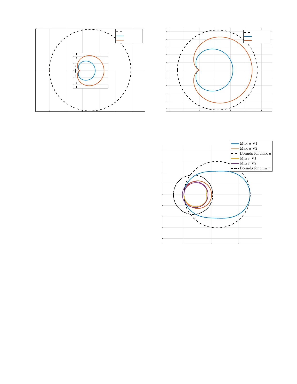
DRAFT : DECEMBER 2017 1 Interior -Conic Polytopic Systems Analysis and Control Alex W alsh, Student Member , IEEE , and James Richard Forbes, Member , IEEE Abstract —Linear parameter varying (LPV) analysis and con- troller synthesis theory r ooted in the small gain and passivity framework currently exist. The study of conic systems encom- passes both small gain and passivity pr operties, and herein, analysis and controller synthesis for polytopic conic systems is consider ed. Linear matrix inequality constraints are given to provide conic bounds for polytopic systems. In addition, given controller conic bounds, a control synthesis method is introduced. The polytopic conic controller is demonstrated on a heat exchanger in simulation, and compared to existing LPV control design techniques. Index T erms —conic systems, gain scheduling, linear parameter varying (LPV) I . I N T R O D U C T I O N Input-output properties and associated stability theorems are indispensable tools to a control systems engineer . In particular , passi vity and small gain properties, as well as their associated input-output stability theorems, are well-kno wn and heavily used in robust, nonlinear , and optimal control. The Passi vity Theorem is commonly used for the robust control of mechanical and electrical systems, especially in the context of robotics [1]. Other robust control strate gies, including H ∞ control, make use of the Small Gain Theorem, which has been used to robustly control aerospace [2], electric, and piezoelectric systems [3]. The Small Gain Theorem is at the heart of robust linear parameter varying (LPV) control. Specifically , the Bounded Real Lemma was extended for application to parameter v ary- ing systems, enabling the statement of sufficient conditions to deriv e stabilizing LPV controllers [4, p. 15]. T wo examples that are particularly relev ant to this paper are [5], [6], where polytopic controller synthesis is discussed. In [5], subcon- trollers at each vertex are synthesized while simultaneously satisfying a global constraint for stability , whereas in [6], subcontrollers at each vertex are first synthesized, and then a global constraint for stability is imposed in an effort to reduce computational comple xities. Initial attempts at deri ving LPV controllers had shortcom- ings such as limits on parameter-variation rates and synthesis complexity , but recent ef forts hav e greatly improved LPV control effecti veness and synthesis tractability [4], [7]–[9]. Nonetheless, LPV plant descriptions are often approximations of nonlinear systems, and a controller synthesized to stabilize one of these approximations is not guaranteed to stabilize A. W alsh is with the Department of Aerospace Engineering, The Univ ersity of Michigan, FXB Building, 1320 Beal Street, Ann Arbor, Michigan, 48109- 2140 USA. J. R. Forbes is with the Department of Mechanical Engineering, McGill Univ ersity , Macdonald Engineering Building, 817 Sherbrooke Street W est, Montr ´ eal, Qu ´ ebec, H3A 0C3, Canada. Email: james.richard.forbes@mcgill.ca. the original nonlinear system [9]. For passiv e systems, the Passi vity Theorem is used to circumvent this problem [10]– [12]. Strictly passi ve controllers can guarantee closed-loop input-output stability of passiv e plants, e ven if an approximate model is used for controller synthesis. Despite advances in control theory and controller synthesis rooted in the Passivity and Small Gain Theorems, relying on these two theorems introduces limitations. For instance, relying on the Small Gain Theorem may lead to conserv ative results o wing to the fact that the analysis relies on the supremum of the operator in question. W eighting transfer functions can be used to emphasize certain frequency bands, but the conservatism still remains. When stabilizing systems using the Passi vity Theorem, plants that are nominally con- sidered passi ve can have so-called passivity violations due to discretization, time-delay , and sensor noise [13], [14]. W ith any one or a combination of these violations, results obtained using the Passivity Theorem may be void. As it turns out, the Conic Sector Theorem is a more general input-output stability theorem, of which small gain and passivity are special cases [15]. Synthesizing a controller with the Conic Sector Theorem can help avoid the conservati ve nature of controllers designed using the Small Gain Theorem, and pro vide a remedy for situations where the plant features a passi vity violation and the P assivity Theorem is not applicable. The design of conic controllers has been studied for linear systems [14], [16], [17]. The design approach considered in [14], [16], [17] be gins by determining the conic bounds of the plant using the Conic Sector Lemma [18], then choosing appropriate conic bounds of the controller using the Conic Sector Theorem [15], and finally synthesizing a linear con- troller that satisfies these conic bounds. A similar approach is undertaken in this paper specific to polytopic systems, which are a type of LPV system. One paper inv estigates the use of conic-sector-based control for LPV systems where conicity is violated for certain values of the parameters [19]. The challenges to o vercome include the fact that currently there are no LMI conditions to determine conic bounds for poly- topic systems, and no synthesis methods for conic polytopic controllers. In short, the two main contrib utions of this paper are provid- ing a means to assess the conic bounds of polytopic systems using an LMI as stated in Theorem 3.1, and a method to design polytopic conic controllers in Section IV. A third contribution is the demonstration of the conic polytopic controller on a heat exchanger . Notation and preliminaries are in Section II, the deri vation of conic bounds for polytopic systems are in Section III, the numerical example is in Section V, and closing remarks are in Section VI. 2 DRAFT : DECEMBER 2017 G 1 G 2 r 1 + u 1 y 1 + − y 2 u 2 r 2 + Fig. 1: Input-output system block diagram. I I . N O T AT I O N A N D P R E L I M I NA R I E S A. Notation A function u ∈ L 2 if k u k 2 = p h u , u i = q R ∞ 0 u T ( t ) u ( t ) dt < ∞ and u ∈ L 2 e if k u k 2 T = p h u , u i T = q R T 0 u T ( t ) u ( t ) dt < ∞ , ∀ T ∈ R ≥ 0 [20]. The matrix 1 is the identity matrix. A “ ? ” indicates symmetry for off-diagonal terms in a matrix. B. Conic Systems Consider a square system G : L 2 e → L 2 e , satisfying − k G u k 2 2 T + ( a + b ) h G u , u i T − ab k u k 2 2 T ≥ β , (1) for all u ∈ L 2 e and T ∈ R ≥ 0 , where β ∈ R and a, b ∈ R , a < b . The system G is interior conic, denoted G ∈ cone[ a, b ] , if (1) holds for some a and b . The system G is strictly interior conic, denoted G ∈ cone( a, b ) , if (1) holds for bounds a + δ and b − δ for some δ > 0 . If a = − γ and b = γ , then (1) reduces to the finite-gain expression k G u k 2 T ≤ γ k u k 2 T + β . (2) If G is linear and β = 0 , then (2) implies k G k ∞ ≤ γ , where k G k ∞ = sup u ∈L 2 e \{ 0 } k G u k 2 T k u k 2 T . Theor em 2.1 (Conic Sector Theor em [15], [16]): Consider the ne gati ve feedback interconnection of tw o square systems, G 1 : L 2 e → L 2 e and G 2 : L 2 e → L 2 e , shown in Fig. 1, where y i = G i u i for i ∈ { 1 , 2 } . The closed-loop system with inputs r = [ r T 1 r T 2 ] T and outputs y = [ y T 1 y T 2 ] T is input-output stable if G 1 ∈ cone[ a, b ] for a < 0 < b and G 2 ∈ cone( − 1 b , − 1 a ) . Input-output stability means that if r ∈ L 2 , then y ∈ L 2 . Cor ollary 2.1 (Small Gain Theor em [21]): Consider the system in Theorem 2.1, where G 1 ∈ cone[ − γ 1 , γ 1 ] and G 2 ∈ cone[ − γ 2 , γ 2 ] . If γ 1 γ 2 < 1 and r ∈ L 2 , then u ∈ L 2 and y ∈ L 2 . Remark 1: Corollary 2.1 demonstrates that the Small Gain Theorem is a special case of the Conic Sector Theorem when the systems composing the negati ve feedback loop are square. Howe ver , the Small Gain Theorem is also applicable to non- square systems [21]. I I I . C O N I C P O LY TO P I C S Y S T E M S A. System Ar chitectur e Recall a matrix polytope is defined as the con vex hull of a finite number of matrices H i , defined as Co { H i , i = 1 , . . . , N } = ( N X i =1 s i H i    s i ≥ 0 , N X i =1 s i = 1 ) . G G c ∆ z w y u p q Fig. 2: Standard problem block diagram with an uncertainty block. G cl ∆ w z p q (a) Closed-loop control frame- work relying on the Small Gain Theorem. G ∆ G c w z y u (b) Closed-loop control frame- work relying on the Conic Sector Theorem. Fig. 3: Upper and lower LFTs for controller synthesis. In this paper , only polytopic systems are examined. Consider the polytopic system sho wn in Fig. 2, gi ven by ˙ x = Ax + B 1 w + B 2 u + B 3 q , (3) z = C 1 x + D 11 w + D 12 u + D 13 q , (4) y = C 2 x + D 21 w , (5) p = C 3 x + D 31 w + D 32 u + D 33 q , (6) where x ∈ R n is the system state, z ∈ R n z is the performance variable, w ∈ R n w is the e xogenous signal that can include noise, y ∈ R m is the measurement variable, p ∈ R n p is the input to the uncertainty block, q ∈ R n q is the output of the uncertainty block, and u ∈ R m is the system input. Each system matrix is a function of a scheduling signal s i , such that     A B 1 B 2 B 3 C 1 D 11 D 12 D 13 C 2 D 21 0 0 C 3 D 31 D 32 D 33     = N X i =1 s i ( σ , x , t )     A i B 1 ,i B 2 ,i B 3 ,i C 1 ,i D 11 ,i D 12 ,i D 13 ,i C 2 ,i D 21 ,i 0 0 C 3 ,i D 31 ,i D 32 ,i D 33 ,i     , (7) where 0 ≤ s i ( σ , x , t ) ≤ 1 , N X i =1 s i ( σ , x , t ) = 1 . (8) The scheduling signals s i ( σ , x , t ) can be a function of time t ∈ R ≥ 0 , a function of state x ∈ R n , or a function of an exogenous signal σ ∈ R n σ . For robust control design using H ∞ -based techniques, the H ∞ norm of the closed-loop system of the plant G and the controller G c , denoted G cl , is determined. Closed-loop input- output stability with ∆ is guaranteed via Theorem 2.1 when W ALSH AND FORBES: INTERIOR-CONIC POL YTOPIC SYSTEMS ANAL YSIS AND CONTR OL 3 k ∆ k ∞ k G cl k ∞ < 1 . The block diagram for this synthesis is described by Fig. 3a. Controller synthesis methods using the Small Gain Theorem are extensiv ely co vered in the literature. For general reference using LMIs see [22], and for polytopic systems, controller synthesis is discussed in [5]. Con versely , for robust control design rooted in the conic- systems framework, which is the focus of this paper, the uncertainty and the plant are lumped together as G ∆ , as shown in Fig. 3b. The conic bounds for the system G ∆ are first determined for u 7→ y , and then appropriate controller bounds are determined via Theorem 2.1 to ensure closed-loop input- output stability . This is also how rob ust control based on the passiv e-systems framework is commonly realized [21]. The Conic Sector Lemma [18] can be used to determine conic bounds for L TI systems. T o apply the Conic Sector Theorem to this robust control design problem the conic bounds of the polytopic system under control must be found. This is addressed in Theorem 3.1 in Section III-B. B. Conic Bounds for P olytopic Systems Conic bounds for a system are defined for a specific input- output pair . For the plant (3)-(6), the input-output pair for conic bounds is u 7→ y , with minimal state space realization G : ( ˙ x = A ( s ) x + B 2 ( s ) u y = C 2 ( s ) x (9) where x ∈ R n , u ∈ R m , y ∈ R m , s = [ s 1 · · · s N ] T , and  A ( s ) B 2 ( s ) C 2 ( s ) 0  = N X i =1 s i ( σ , x , t )  A i B 2 ,i C 2 ,i 0  , (10) where s satisfies (8). The feedthrough matrix, D 22 , is assumed to be zero as physical systems e xhibit some sort of roll-off in gain at higher frequency . If a model does contain a D 22 matrix, the measurement y can be filtered to remov e the feedthrough term. Lemma 3.1: Giv en y ( t ) = P N i =1 s i ( σ , x , t ) y i ( t ) , where y ( t ) ∈ L 2 e , y i ( t ) = C 2 ,i x ( t ) , and where scheduling signals satisfy (8), then − k y ( t ) k 2 2 T ≥ N X i =1 −    p s i ( σ , x , t ) y i ( t )    2 2 T . (11) Pr oof: See the Appendix. Theor em 3.1: Consider the system y = G u described by (9), where A ( s ) , B ( s ) , and C ( s ) satisfy (8) and (10). For a, b ∈ R , a < 0 < b , if the LMI in P  P A i + A T i P + C T 2 ,i C 2 ,i PB 2 ,i − a + b 2 C T 2 ,i ? ab 1  = −  L T i W T i   L i W i  ≤ 0 (12) is satisfied for some real matrices P = P T > 0 , L i and W i for i = 1 , . . . , N , then the system G is in cone[ a, b ] . Pr oof: In this proof, the argument s associated with ( A ( s ) , B ( s ) , C ( s )) is dropped for brevity . First note that (12) implies P A i + A T i P + C T 2 ,i C 2 ,i = − L T i L i , PB 2 ,i − a + b 2 C T 2 ,i = − L T i W i , ab 1 = − W T i W i . (13) Consider the time deriv ati ve of the L yapunov-like function V = 1 2 x T Px , ˙ V = 1 2 x T ( P A + A T P ) x + x T PBu . (14) Substituting (13) into (14) yields ˙ V = N X i =1 s i  − 1 2 x T C T 2 ,i C 2 ,i x + x T  a + b 2  C 2 ,i u − 1 2 x T L T i L i x − x T L T i W i u − 1 2 u T W T i W i u + 1 2 u T W T i W i u  = N X i =1 s i  − 1 2 y T i y i − 1 2 ( L i x + W i u ) T ( L i x + W i u )  − 1 2 ab u T u +  a + b 2  y T u . (15) Integrating (15) in time from 0 to 0 < T < ∞ gives V ( T ) − V (0) = N X i =1  − 1 2 k √ s i y i k 2 2 T − 1 2 k √ s i ( L i x + W i u ) k 2 2 T  − ab 2 k u k 2 2 T +  a + b 2  h y , u i T . Rearranging yields − N X i =1 k √ s i y i k 2 2 T + ( a + b ) h y , u i T − ab k u k 2 2 T = +2( V ( T ) − V (0)) + N X i =1 k √ s i ( L i x + W i u ) k 2 2 T . (16) Since 2( V ( T ) − V (0)) + P N i =1   √ s i ( L i x + W i u )   2 2 T ≥ − 2 V (0) , using Lemma 3.1 reduces (16) to − k y k 2 2 T + ( a + b ) h y , u i T − ab k u k 2 2 T ≥ β , (17) where β = − 2 V (0) only depends on initial conditions. Comparing (17) to (1) proves Theorem 3.1. Cor ollary 3.1: Consider the system y = G u described by (9). For a, b ∈ R , a < 0 < b , if the LMI in ˜ P  ˜ PA i + A T i ˜ P + 1 b C T i C i ˜ PB i − 1 2  a b + 1  C T i ? a 1  ≤ 0 (18) is satisfied for i = 1 , . . . , N , and ˜ P = ˜ P T > 0 , then the system G is in cone[ a, b ] . Pr oof: Multiplying (12) by 1 b > 0 results in  1 b P A i + A T i P 1 b + 1 b C T i C i 1 b PB i − 1 2  a b + 1  C T i ? − a 1  ≤ 0 . 4 DRAFT : DECEMBER 2017 Using the change of variable ˜ P = 1 b P yields (18). Since change of variable and multiplication are re versible, (18) also implies (12). Thus, if G satisfies Corollary 3.1, then G also satisfies Theorem 3.1. Both Theorem 3.1 and Corollary 3.1 are sufficient condi- tions for G ∈ cone[ a, b ] . Corollary 3.1 is a reformulation of Theorem 3.1, and may be useful in situations with a lar ge b . A large b can cause (12) to become ill-conditioned, whereas a lar ge b does not cause problems for (18). C. Determining Conic Bounds The matrix inequality (12) is nonlinear in a and b , and thus solving for an a and b directly gi ven the polytopic plant G is not possible. Three methods of determining tight bounds a and b exists. The y consist of 1) fixing a = −∞ , minimizing b , then fixing b , and maximizing a , 2) fixing b = ∞ , maximizing a , then fixing a , and minimiz- ing b , and 3) defining the conic radius r = b − a 2 and conic centre, c = a + b 2 , and then minimizing the conic radius. As [14] shows for the L TI case, each method yields different conic bounds. In the polytopic case, the same holds true. Fix- ing b = ∞ , and then maximizing a is preferred to determine plant conic bounds because this results in a controller with the least conservati ve gain. T o understand why , note that the controller conic bound b c = − 1 a is related to controller gain, and thus an a v alue as close to zero as possible is desired. When, b is set to ∞ , Corollary 3.1 is used. T o determine conic bounds using the radius and centre, r and c respectiv ely , consider that  P A i + A T i P + C T i C i PB i − c C T i ? − κ 1  ≤ 0 (19) is equi valent to (12), where κ = − ab . Note that r 2 = ( a − b ) 2 4 = ( a + b ) 2 − 4 ab 4 = c 2 + κ, (20) and thus minimizing (20) results in the minimum conic radius. The equiv alent method for an L TI system is found in [16]. Since (20) is quadratic, it can be transformed to a linear objectiv e along with an LMI constraint by introducing a variable z , and then minimizing z subject to the constraint  z − κ c ? 1  ≥ 0 , (21) where (21) is deriv ed from z ≥ c 2 + κ using the Schur complement [23]. I V . D E S I G N O F P O L Y T O P I C C O N I C C O N T RO L L E R S Passi vity-based synthesis for affine systems is discussed in [12]. The conic-polytopic controller synthesis considered in this paper is an adaptation of the synthesis methods presented in [12], [14], [17]. The goal is to determine a set of controller matrices,  A c ( s ) B c ( s ) C c ( s ) 0  = N X i =1 s i ( σ , x , t )  A c ,i B c ,i C c ,i 0  , (22) where the signals s i satisfy (8). In particular , an H ∞ controller is synthesized at each verte x of the polytope, and then the closest controller in an H 2 sense that satisfies conic constraints giv en by (12) is determined. Associated assumptions are 1) ( A i , B 2 ,i , C 2 ,i ) is stabilizable and detectable, and 2) D 22 = 0 . The resulting state space matrices from the H ∞ synthesis are ( A c ,i , L i , K i , 0 ) , where A c ,i from the H ∞ synthesis is also the A c ,i of the conic controller given in (22). The matrix C c ,i in (22) is set to C c ,i = K i . The B c ,i matrix is determined by minimizing the H 2 norm of the difference between the H ∞ controller and a controller that satisfies (12). Specifically , this optimization problem is gi ven by minimizing J ( Π c , B c , 1 , . . . , B c ,N ) = N X i =1 tr( B c ,i − L i ) T W i ( B c ,i − L i ) , (23) subject to    Π c A T c ,i + A c ,i Π c B c ,i C c ,i Π c ? − ( a c − b c ) 2 4 b c 1 − a c + b c 2 1 ? ? − b c 1    < 0 , (24) for i = 1 , . . . , N , where (24) is derived from Corollary 3.1. The deriv ation is omitted for brevity , but see [14] for a similar deriv ation. Equation (18) cannot be used for controller synthesis since it is bilinear in B and P . The matrix W i is the observ ability Grammian that satisfies A T c ,i W i + W i A c ,i + C T c ,i C c ,i = 0 . The objective function (23) is chosen because when the difference between B c i and L i subject to the weight W i is minimized, the dif ference between the H ∞ controller and the controller that satisfies (12) is minimized in an H 2 sense. The quadratic function (23) can be transformed to a linear function and an LMI constraint giv en by ˆ J ( ν , Z , Π c , B c , 1 , . . . , B c ,N ) = ν, (25) constrained by ν ≥ tr( Z ) , (26) and      Z ( B c , 1 − L 1 ) T · · · ( B c ,N − L N ) T ? W − 1 1 0 0 . . . ? . . . . . . ? ? ? W − 1 N      ≥ 0 . (27) Determining B c ,i is summarized by Problem 4.1. Pr oblem 4.1: The problem to determine B c ,i for i = 1 , . . . , N is gi ven by minimizing (25), subject to (24), (26), and (27).  V . N U M E R I C A L E X A M P L E A numerical example using a heat exchanger is used to highlight the usage of the polytopic conic controller . The conic controller is compared to the polytopic LPV controller from [5], which uses the Small Gain Theorem for robust closed-loop stability . W ALSH AND FORBES: INTERIOR-CONIC POL YTOPIC SYSTEMS ANAL YSIS AND CONTR OL 5 T ABLE I: Heat e xchanger properties Parameter Unit Cold Fluid Hot Fluid U J s · m 2 · ◦ C 2411 . 8 2411 . 8 A m 2 48 . 4 48 . 4 v c, i , v h, i m 3 / s 0 . 04 0 . 10 v c, f , v h, f m 3 / s 0 . 02 0 . 06 ρ c , ρ h kg / m 3 · 10 3 3 . 50 3 . 72 c pc , c ph J kg · ◦ C 481 . 8 499 . 0 V c , V h m 3 · 10 − 2 15 . 8 57 . 8 T o c, i ◦ C 9 . 3 – T o c, f ◦ C 25 – A. System Description Consider the linearized model of a heat exchanger described by [24, pp. 55–60], with properties listed in T able I. The non- homogeneous dif ferential equation describing the dynamics of the heat exchanger is giv en by ˙ T = A p T + B p T i h + W T i c , (28) where A p = " − v c ( t ) V c − U A c pc ρ c V c U A c pc ρ c V c U A c ph ρ h V h − v h ( t ) V h − U A c ph ρ h V h # , (29) B p =  0 − v h ( t ) V h  , W =  − v c ( t ) V c 0  , T =  T o c ( t ) T o h ( t )  . (30) In this model, the input cold stream T i c is constant, and the outlet temperature T o c is to be regulated. The hot inlet temperature T i h is the control input, and the flow rates of the hot and cold fluids, v c ( t ) and v h ( t ) respectively , are time varying. In particular , cold and hot stream flow rates are v c ( t ) = φ ( t, v c, i , v c, f ) and v h ( t ) = φ ( t, v h, i , v h, f ) , where t f = 20 s, and where φ ( t, x i , x f ) =        x i , t ≤ 0 , x i + ( x f − x i )  3  t t f  2 − 2  t t f  3  , 0 ≤ t ≤ t f , x f , t f ≤ t. (31) The desired cold output temperature is giv en by T o c, d ( t ) = φ ( t, T o c, i , T o c, f ) T o realize a linear system with desired out- put y = 0 , the system (28) is approximated by using the change of variables x = T + η + [ ν ν ] T , u = T i h + ν , and y =  1 0  ( T + η ) + ν , where η = ( A p + W  1 0  ) − 1 W ( T i c − T o c, f ) , and ν =  1 0  η − T o c, f . When fluid-flo w is constant, ˙ x = ˙ T . The resulting state-space realization is determined using (31). The matrices A and B 2 are A = 2 X i =1 s i ( σ , x , t ) A i , B 2 = 2 X i =1 s i ( σ , x , t ) B 2 ,i , where s 1 = φ ( t, 1 , 0) , and s 2 = 1 − s 1 = φ ( t, 0 , 1) . The matrices A 1 and B 2 , 1 are defined by ev aluating A p and B p in (29)-(30) at v c, i and v h, i . The matrices A 2 and B 2 , 2 are T ABLE II: Conic bounds of the heat exchanger model. Plant Conic Max a Conic Min r k ∆ k ∞ δ = 0 cone[ − 0 . 06 , 98 . 9] cone[ − 0 . 14 , 0 . 38] 0 δ = 0 . 5 cone[ − 0 . 04 , 97 . 4] cone[ − 0 . 09 , 0 . 24] 0 . 057 δ = − 1 cone[ − 0 . 08 , 99 . 4] cone[ − 0 . 19 , 0 . 52] 0 . 23 defined by ev aluating A p and B p in (29)-(30) at v c, f and v h, f . The matrix C 2 is constant, where C 2 = [1 0] . B. Robust Contr ol Design The parameters in A p are generally uncertain. For example, U is uncertain due to CaCO 3 formation [24, p. 31]. The uncertain ¯ A matrix is modelled as ¯ A = A + A δ , where A δ = δ " U A c pc ρ c V c − U A c pc ρ c V c − U A c ph ρ h V h U A c ph ρ h V h # , δ ∈ R . The system for rob ust control design is then ˙ x = Ax + B 2 u + q , y = C 2 x , p = x , (32) where the uncertainty block is gi ven by q = A δ p , and thus ∆ = A δ . The weighting matrices for rob ust control design using (32) are B 3 = 1 , C 3 = 1 , D 23 = 0 , D 32 = 0 . (33) Other weighting combinations are possible, such as by factor- ing A δ , with factorization B 3 C 3 = A δ or B 3 C 3 = δ − 1 A δ , and then by setting ∆ = 1 or ∆ = δ 1 . In some cases, this may provide a numerically simpler controller synthesis, but in the heat e xchanger example, no significant controller improv ements were found. T able II shows the heat e xchanger’ s conic sectors and || ∆ || ∞ for v arious values of δ . A value of δ = 0 . 5 is equiv alent to halving the heat exchanger’ s area, such as during CaCO 3 buildup. A value of δ = − 1 doubles the heat exchanger’ s area. Using the design method for an LPV controller from [5], the input must be filtered to obtain a constant B 2 matrix. A first- order filter with a cutoff frequency of 2 rad/s is implemented on the input of the system, which adds system states. Design- ing the polytopic LPV controller using the weights from (33) results || G cl || ∞ = 16 . 67 . Recall that for robust closed-loop stability via the Small Gain Theorem, || G cl || ∞ < 1 / || ∆ || ∞ . This means that stability can be guaranteed via the Small Gain Theorem for δ = 0 . 5 , b ut cannot be guaranteed for δ = − 1 . The conic bounds of the heat exchanger are found using Theorem 3.1. The Nyquist plots of G at the vertices of the polytope are shown in Fig. 4, as well as a circle that denotes the conic bounds. Notice that the plant lies well within the conic bounds determined by Theorem 3.1. The Nyquist plot of the vertices is shown in Fig. 5 when the conic radius is minimized. In this plot, the black dashed circle is much tighter than when maximizing a . This would seem like tighter conic bounds and thus improv ed controller performance, b ut the more negativ e a leads to a decreased b c , and thus yields a controller with more conservati ve gain 6 DRAFT : DECEMBER 2017 0 20 40 60 80 100 Real Axis -50 0 50 Imaginary Axis 0 0.2 0.4 Real Axis -0.2 -0.1 0 0.1 0.2 Imaginary Axis Plant Cone Vertex 1 Vertex 2 Fig. 4: Plant conic boundary and plant Nyquist plot. Embedded plot is a zoomed-in v ersion to emphasize the plant’ s Nyquist plot at the vertices. and inferior performance. T o robustly stabilize the plant, the largest cone that captures both the nominal and perturbed plant must be considered, thus the cone for controller design is cone[ − 0 . 19 , 0 . 52] for minimizing r and cone[ − 0 . 08 , 99 . 4] for maximizing a . The weights given by (33) are used to design the H ∞ controllers at each vertex. These controllers are used for controller synthesis, as discussed in Section IV. T o analyze the utility of forcing the H ∞ controllers at each v ertex to satisfy Theorem 2.1, the H ∞ controllers at each verte x are linearly interpolated to form an H ∞ gain-scheduled controller . This controller has no stability or performance guarantees when in closed-loop with the heat exchanger . The Nyquist plots of the H ∞ controller at each vertex and the conic controller at each verte x, synthesized using maximum plant a , are shown in Fig. 7. The gain of the interpolated H ∞ controller is much larger than the gain of the conic controllers at each vertex. When synthesizing the conic controller , the effect of the synthesis decreases gain of the controller so that the controller lies within cone( a c , b c ) . The gain at both vertices are not the same. The gain at vertex 1 of the H ∞ controller is smaller than at v ertex 2, and this is rev ersed for the conic case. Fig. 6 sho ws the conic bounds for the controller synthesized with maximum plant a and minimum plant r . The b c bound, which is related to the upper limit on controller gain, is approx- imately 2 . 5 times larger when using the bounds determined by maximum a than by minimum r . It is expected that the controller with the larger design freedom exhibits superior closed-loop performance, that is the RMS error of T o c should be less for the max a controller than the min r controller . C. Numerical Results Numerical results are shown in Fig. 8, and the case δ = − 1 is omitted for brevity . The root-mean square (RMS) values of the error of the cold outlet temperature are shown in -0.2 -0.1 0 0.1 0.2 0.3 0.4 Real Axis -0.25 -0.2 -0.15 -0.1 -0.05 0 0.05 0.1 0.15 0.2 0.25 Imaginary Axis Plant Cone Vertex 1 Vertex 2 Fig. 5: Plant conic boundary and plant Nyquist plot with minimum conic radius. 0 5 10 Real Axis -8 -6 -4 -2 0 2 4 6 8 Imaginary Axis Fig. 6: Nyquist plot of controllers at vertices of polytope synthesized using maximum plant a and minimum plant r conic bounds. T able III. At δ = 0 . 5 , the area for heat exchange halves. The performance of all controllers improv e with δ = 0 . 5 , which implies that not all uncertainty degrades performance. When δ = − 1 , the opposite is true and the performance of all controllers deteriorates. Howe ver , comparing the change of performance of each controller with respect to δ yields interesting results. The standard deviation between the RMS errors is sev en times less for the conic controller design than with the H ∞ -based LPV design. This is partly expected because conic controllers exhibit a similar level of robustness for linear control design [14]. This lack of sensitivity to model uncertainty highlights the benefits of conic-sector-based control. The conic controller that uses the maximum a plant sector W ALSH AND FORBES: INTERIOR-CONIC POL YTOPIC SYSTEMS ANAL YSIS AND CONTR OL 7 0 10 20 30 40 50 Real Axis -30 -20 -10 0 10 20 30 Imaginary Axis Fig. 7: Nyquist plot of H ∞ controller and the conic controller at each vertex of the polytope. The controller circle plots the conic bounds of the controller . T ABLE III: RMS error of T o c − T o c, d , ◦ C Plant H ∞ Conic Max a Conic Min r LPV δ = 0 1 . 13 0 . 612 0 . 912 1 . 19 δ = 0 . 5 0 . 782 0 . 606 0 . 850 0 . 832 δ = − 1 1 . 72 0 . 721 1 . 047 1 . 68 std. de v . 0 . 477 0 . 065 0 . 100 0 . 424 has superior performance that the conic control that uses the minimum r plant sector . This is expected since the maximum a plant sector controller has larger conic bounds, and thus less design restriction. Both conic controllers hav e superior performance compared to the LPV controller, but this can be explained since the LPV controller was designed to maximize robustness instead of performance. For δ = 0 and δ = 0 . 5 , the H ∞ controller actually performs better than the LPV controller . This may be e xplained by the fact that for polytopic controller design, a common L yapunov matrix is required, which is a source of conservatism. The interpolated H ∞ is synthesized at the vertices, and even though it has no guarantee to stabilize the closed-loop system, instability was not the result. Howe ver , with a different set of weighting matrices, in simulation, the interpolated H ∞ controller lead to poor closed-loop performance, and even closed-loop instability . V I . C O N C L U D I N G R E M A R K S This paper provides LMI conditions to determine conic bounds for interior -conic polytopic systems. This paper also provides a method that synthesizes a polytopic controller subject to conic bounds. In simulation, the synthesized conic controllers e xhibit v ery little sensitivity to model uncertainty . For conic-sector-based robust control, the controller is forced to satisfy conic bounds to ensure closed-loop stability with G ∆ . For traditional robust control, the controller is designed such that G cl satisfies the small gain condition with respect to the uncertainty block, ∆ . Since the conic-sector and small gain methods approach robustness in a dif ferent manner , this paper only provides an indirect comparison. In the future, it is of interest to design G cl to satisfy conic bounds, or to hav e G c satisfy the small gain condition with respect to G ∆ so that uncertainty is approached in a similar manner . A common L yapunov matrix is required for both these methods, which is a source of conservatism when determin- ing conic bounds for the plant, and when synthesizing the controller . This conservatism may provide undesirably large conic bounds for the plant, which would lead to less control design freedom. When synthesizing the conic controller , the common L yapunov matrix may prevent the controller to use the full allow able controller cone. The effects and methods to mitigate the common L yapunov matrix is an area of future research. A P P E N D I X P RO O F O F L E M M A 3 . 1 This Appendix presents the proof of Lemma 3.1. Each element of y is gi ven by y j ( t ) = P N i =1 s i ( σ , x , t ) y ij ( t ) , whose square results in y 2 j ( t ) =      N X i =1 s i ( σ , x , t ) y ij ( t )      2 , =      N X i =1 p s i ( σ , x , t )  p s i ( σ , x , t ) y ij ( t )       2 . Using the Cauchy-Schwartz Inequality yields y 2 j ( t ) ≤ N X i =1    p s i ( σ , x , t )    2 ! N X i =1    p s i ( σ , x , t ) y ij ( t )    2 ! = N X i =1 s i ( σ , x , t ) ! N X i =1 ( p s i ( σ , x , t ) y ij ( t )) 2 ! = N X i =1 s i ( σ , x , t ) y 2 ij ( t ) ! . T aking the sum from j = 1 to m , and then rearranging yields m X j =1 y 2 j ( t ) ≤ m X j =1 N X i =1 s i ( σ , x , t ) y 2 ij ( t ) ! y T ( t ) y ( t ) ≤ N X i =1 s i ( σ , x , t ) m X j =1 y 2 ij ( t ) = N X i =1 s i ( σ , x , t ) y T i ( t ) y i ( t ) . 8 DRAFT : DECEMBER 2017 0 10 20 30 40 50 60 70 80 0 10 20 30 0 10 20 30 40 50 60 70 80 20 40 60 80 100 120 0 10 20 30 40 50 60 70 80 0 100 200 0 10 20 30 40 50 60 70 80 0 5 (a) Nominal plant with δ = 0 . 0 10 20 30 40 50 60 70 80 0 10 20 30 0 10 20 30 40 50 60 70 80 20 40 60 80 100 120 0 10 20 30 40 50 60 70 80 0 100 200 0 10 20 30 40 50 60 70 80 0 5 (b) Modified plant with δ = 0 . 5 . Fig. 8: Simulation results to track T o c , with input T i h of the heat exchanger . Integrating both sides in time from 0 to T in time yields Z T 0 y T ( t ) y ( t ) d t ≤ N X i =1 Z T 0 s i ( σ , x , t ) y T i ( t ) y i ( t ) d t k y ( t ) k 2 2 T ≤ N X i =1    p s i ( σ , x , t ) y i ( t )    2 2 T . (34) Multiplying both sides of (34) by − 1 yields (11). R E F E R E N C E S [1] R. Ortega, J. Lor ´ ıa Perez, P . Nicklasson, and H. Sira-Ramirez, P assivity- Based Contr ol of Euler-Lagrang e Systems: Mechanical, Electrical, and Electr omechanical Applications . London; New Y ork: Springer, 1998. [2] E. Lavretsky and K. A. W ise, Rob ust and Adaptvie Contr ol: W ith Aer ospace Applications . London, United Kingdom: Spring-V erlag, 2013. [3] B. M. W en, Robust and H ∞ Contr ol . London, United Kingdom: Spring- V erlag, 2000. [4] J. Mohammadpour and C. W . Scherer, Control of Linear P arameter V arying Systems with Applications . Boston, MA: Springer , 2012. [5] P . Apkarian, P . Gahinet, and G. Becker, “Self-scheduled H ∞ control of linear parameter-varying systems: a design example, ” Automatica , vol. 31, pp. 1251–1261, 9 1995. [6] F . D. Bianchi and R. S. P . na, “Interpolation for gain-scheduled control with guarantees, ” Automatica , v ol. 47, pp. 239–243, 2011. [7] P . Apkarian and R. Adams, “ Advanced gain-scheduling techniques for uncertain systems, ” IEEE T ransactions on Contr ol Systems T echnology , vol. 6, no. 1, pp. 21–32, 1996. [8] W . J. Rugh and J. S. Shamma, “Research on gain scheduling, ” A uto- matica , v ol. 36, pp. 1401–1425, 2000. [9] C. Hoffmann and H. W erner, “ A survey of linear parameter-v arying con- trol applications v alidated by experiments or high-fidelity simulations, ” IEEE T ransactions on Contr ol Systems T echnology , vol. 23, no. 2, 2014. [10] A. W alsh and J. R. F orbes, “ A very strictly passiv e gain-scheduled controller: Theory and experiments, ” IEEE/ASME Tr ansactions on Mechatr onics , vol. 21, no. 6, pp. 2817–2826, 2016. [11] A. W alsh and J. R. Forbes, “ Analysis and synthesis of input strictly passiv e gain-scheduled controllers, ” Journal of the F ranklin Institute , vol. 343, no. 3, pp. 1285–1301, 2017. [12] A. W alsh and J. R. Forbes, “V ery strictly passive controller synthesis with affine parameter dependence, ” IEEE T ransactions on Automatic Contr ol , 2017. [13] J. R. Forbes and C. J. Damaren, “Synthesis of optimal finite-frequency controllers able to accommodate passivity violations, ” IEEE T ransac- tions on Control Systems T echnology , vol. PP , no. 99, pp. 1–1, 2012. [14] L. J. Bridgeman and J. R. Forbes, “Conic-sector-based control to cir- cumvent passivity violations, ” International Journal of Contr ol , vol. 87, no. 8, pp. 1467–1477, 2014. [15] G. Zames, “On the input-output stability of time-varying nonlinear feedback systems part I & II, ” IEEE Tr ansactions on Automatic Contr ol , vol. 11, no. 2, pp. 229–231, 1966. [16] S. Joshi and A. Kelkar , “Design of norm-bounded and sector-bounded lqg controllers for uncertain systems, ” Journal of Optimization Theory and Applications , vol. 113, no. 2, pp. 269–282, 2002. [17] L. J. Bridgeman, R. J. Caverly , and J. R. Forbes, “Conic-sector-based controller synthesis: Theory and experiments, ” in Proc. 2014 American Contr ol Confer ence (ACC) , (Portland, Oregon, USA), 2014. [18] S. Gupta and S. M. Joshi, “Some properties and stability results for sector-bounded lti systems, ” in Proc. 33rd Confer ence on Decision and Contr ol , v ol. 3, (Lak e Buena V ista, FL), pp. 2973–2978, 1994. [19] S. Sivaranjani, J. R. Forbes, P . Seiler, and V . Gupta, “Conic-sector-based analysis and control synthesis for linear parameter varying systems, ” IEEE Contr ol Systems Letters , vol. 2, no. 2, pp. 224–229, 2018. [20] C. A. Desoer and M. V idyasagar , F eedback Systems: Input-Output Pr operties . New Y ork, NY : Academic Press., 1975. [21] B. Brogliato, R. Lozano, B. Maschke, and O. Egeland, Dissipative Systems Analysis and Control Theory and Applications . London: Springer , 2 ed., 2007. [22] G. E. Dellerud and F . G. Paganini, A Course in Robust Contr ol Theory: A Con vex Appr oach . New Y ork, NY : Springer-V erlag, 2000. [23] S. P . Boyd, Linear matrix inequalities in system and control theory . Philadelphia: Society for Industrial and Applied Mathematics, 1994. [24] K. M. Hangos, J. Bokor, and G. Szederk ´ enyi, Analysis and Control of Nonlinear Pr ocess Systems . London, United Kingdom: Springer, 2004.