Predictive Maintenance in Photovoltaic Plants with a Big Data Approach

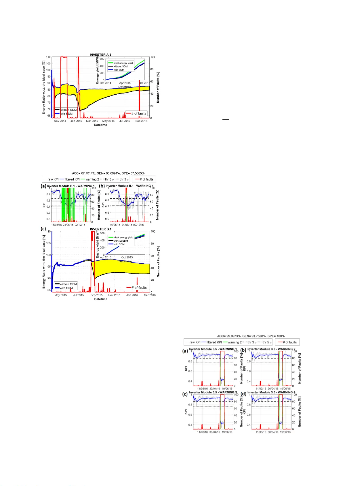
PREDICTIVE MAINTENANCE IN PHOTOVOLTAIC PLANTS WITH A BIG DATA APPROACH Alessandro Betti † , Maria Luisa Lo T rovato ‡ , Fabio Salvatore Leonardi ‡ , Giuseppe Leotta ‡ , Fabrizio Ruffini † and Ciro Lanzetta † † i-EM srl , via Aurelio Lam predi 45, Livorno (Italy) ‡ Enel Green Power SPA , Viale Regina Margherita 125, Rome (Italy) ABSTRACT: This paper presents a n ovel and flexible solution for fault p rediction based on data collected from SCADA s ystem. Fault prediction is off ered at two diff erent levels base d on a data-driven approach: (a) generic fault/status prediction and (b) specific fault class prediction, implemented by means of two different machine learning based modules built on an unsupervised clustering algorithm and a Pattern Recognition Neural Ne twork, respectively. Model has been ass essed on a park of six photo voltaic ( PV ) plants up to 10 MW a nd on more than one hundred inve rter modules of three different techn ology brands. T h e results indicate that th e proposed method is ef fective in (a) p redict ing incipient generic f aults up to 7 days in advance w ith sensitivity up to 95% and (b) antici pating dama ge of spec ific fa ult classes with times ranging f ro m few hours up to 7 days. T he model is easily deplo yable for on -line monitoring of anomalies on new PV plants and t echn ologies, requiring only the availability of historical SCADA and f ault data, f ault taxonomy and inverter electrical datasheet. Keywords: Data Mining, Fault Prediction, Inverter Module, Key P erformance Indicator, Lost Production 1 INTRODUCTION The provision of a Preventive Ma intenance strategy is emerging now adays as an esse ntial field to keep high technical and ec onomic performances of solar PV plants over ti me [1]. Analytical monitoring sy stems have been installed therefore worldwide to timely detect po ssible malfunctions through the assessm ent of PV system performances [2-3]. However, high customization costs, the need of collecting a great nu mber of ph ysical variables and of a stable Internet connectio n on field ge nerally limit their effectiveness, especially for farms in remote places with unreliable communication infrastructures. The lack of a predictive c omponent in the maintenance strategy is als o a hindrance to minimize do wntime costs. In order to keep lower the implementation costs and m od el complexity, statistical methods based on Data Mining are recently emerging a s a v ery prom ising approach bot h for fault prediction and early detection. Ho weve r, while the Literature is mainly focusing on equipment level f ailures in wind farms [ 4-5], research for PV plants is still in an early stage [6]. The present paper d escribes an innovative and versatile solu tion for inverter level fault prediction based on a data-driven approach, already test ed with remarkable performances on six PV plants of variable size up to 10 MW located i n Romania and Gre ece and th ree d ifferent inverter technologies (Table 1). Th e proposed approach is easily portable on different plants and technologies and simplifies the up date process to follow the PV plant evolution. 2 METHODOLOGY The model is composed b y two parallel modules both being capable of predicting incipient fa ults, but differing for the level of details provided and the rem ainin g operational time after first indication of fault: a Supervision-Diagnosis Model (SDM) based on a Self- Organizing Map (SOM) predicting generic failures through a m easure of d eviations from normal operation , and a Short-Term Fault Prediction Model (FPM) base d on artificial Neural Network (NN) addressing th e Table 1 : list of tested PV plants. Plant Number # of Inverter Modules Inverter Manufacturer Number Max Active Power (K W) Plant Nominal Power (M W) 1 35 1 385 9.8 2 3 4 5 6 7 2 25 34 10 1 2 3 3 3 385 731.6 183.4 183.5 183.4 2.8 1.63 4.9 6.0 1.99 prediction of specific fault classes. The main steps of the model workflow are described in the following. 2.1 Data and Alarm Logbook Import Historical data extracted from 5-min averaged SCADA data (Table 2) and inverter manufacturer electrical parameters for the on -site inverter technology are first collected to train the m odel . SCADA lo gbooks, as well as fault taxonomy, are also imported for offline performance assess ment and n ormal train ing period selection in the case of the SDM, and for NN training for the FPM. Logbook import is achieved by matching fault classes listed in the fault taxono my, which includes also fault severity, to the fault o ccurrences recorded in logbooks and discretizing them o n the timestam p grid of SCADA data. In particular, a k -th fa ult is assigned t o timestamp   if the following condition occurs:             , (1) where   (   ) are the initial (final) instant of f ault event. Then SCA D A data labelling is realized by Table 2 : electrical and environmental input S CADA d ata (GHI (GTI): Global Horizontal (Tilted) Irradiance). DC Electrical tags AC Electrical tags Temperature tags Irradiance tags Current (I DC ) Current (I AC ) Internal (T int ) GTI Voltage (V DC ) Voltage (V AC ) Panel (T mod ) GHI Power (P DC ) Power (P AC ) Ambient (T amb ) assigning fault codes (as integer numbers) to SCADA d ata. In the case of concurrent fault events, a prioritization rule is adopted co nsidering only the most severe fault an d, if necessary, the most frequent fault in that day. 2.2 Data Preprocessing AC power (P AC ) depends primarily on the level of solar irradiance (GTI) and, secondarily, on ambient temperature (T amb ). A first-order regression of signals GTI and P AC applied o n train ing set samples allo ws to remove outliers corresponding to the furthest points from fitting:               󰇛      󰇜 , where m and b are the slope and the intercept, respectively, computed by a least squares appro ach and thr is the threshold set by a trial and error process. Further preprocessing steps include removal of d ays with a large amount of missing data, setting periodic tags to 0 in the ni ghttime , data range check and removal of unphysical plateaus. 2.3 Data Imputation Missing instances in test set are imputed by means of a k -Nearest Neighbors ( k -NN) a lgorithm u sing th e training set as the reference historical dataset, selec ting nearest neighbors according to the Euclidean distance and exploiting hyperbolic weights. 2.4 Feature Engineering: Data De-trending and Scaling In order to rem ove th e season-depend ent variability from input data, a de-trending procedure has been app lied by f ollowing customized app roaches for each tag. T mod training data have been d e-trended by means of th e least squares method to find the best line T fit against T amb and selecting on ly low GTI sam ples to remove the effect of panel heating due to sunlight:                , (2) where             is the f itting ,   is the regression slope and   is the intercept. All the remainin g input tags, but DC and A C voltages, have been de-trended according to a classical Mo ving Average (M A) s moothing to compute the trend component and applying an additive model for time serie s deco mposition. In both cases also test instances have been de- tr ended by means of a moving window m a sk 1 -day lon g f or tracking of ti me-varying input patterns. Finally, input data normalization is performed to avoid unbalance between h eterogeneous tags. 2.5 Data Processing: the Supervision Model (SDM) SDM has been built by means of an unsupervised clustering approach based on a 20 ×20 Self-Organizing Map (SOM) a lgorithm (Figure 1) perf o rming a non - Figure 1 : workflow of the Mod el SDM (SOM based) and FPM (NN based) from SCADA in put tags to model outputs available in an operator dashboard. Figure 2 : (a)     and (b )          con sidering the full training and test p hases. The larger the occupancy difference in (b), the sm aller the contribution to KPI value (Eq. (3)). linear mapping from a n-dimension al space (n=11) to a 2- dimensional space with an online weight update rule [7] and trained on a normal operation period, id entified by a time interval, through a competitive learning pro cess. SOM h as the valuable property of p reserving inp ut topology: neighbor neurons in the SOM la yer respo nd to similar input vectors. As a consequence, a change in th e distribution of input instances, d ue f o r exam ple to inverter malfunction, leads to a different data mapping in the output grid . A m ultivariate statistical process con trol analysis in the form of a con trol chart m a y be there fore built to detect this change in the patterns distribution. A Key P erformance Indicator (KPI) has been defined as in Eq. (3), measuring a process variation at generation unit level from the normal state towards abn ormal operating conditions when a threshold is crossed:          󰇻      󰇻 󰇻      󰇻 , (3 ) where sums run on the SOM cells,              is th e normalized number of input patterns mapped i n to the cell (i,j) in t he training p hase and               is the normalized number o f input patterns m apped in to the cell (i, j) in a 24 -hours test phase (Figure 2 ). The ratio factor in Eq. (3) penalizes large deviation s from th e training operating conditions: indeed if  󰇛    󰇜        then    , and if          󰇛           , or viceversa), then    . From a phy sical point of view, Eq. (3) is a robust indicator detecting changes in the underlying no n-linear dynamics of the generation unit from normal status, represented by    . To remove the seasonality pattern from Eq. (3 ) due to time-varying number of daytime instances, a KPI de - trending pr ocedure h as been followed by means of a linear regression of b oth signals to compute th e KP I tren d and selecting the de-trended component     by assuming a multiplicative decomposition               . Once Table 3: rules for switching ON o f the 4 warning levels (w) of the SDM (d: day). Warning Level (w) Crossing of Threshold KPI Derivative Persistence 1    < 0 1 d 2    < 0 2 d of w 1 3    < 0 1 day 4    < 0 2 d of w 3 the de-trended KPI is available, a low-pass MA filter with a 4-weeks long w indow is applied. F inally, four warning levels of d ifferent severity are computed based on thresholds crossing and time p ersistence ru les (Table 3 ). Model performances have been evaluated by means of usual classification metrics (accuracy, sensitivity and specificity) exploiting th e alarm logbook knowledge and assigning a predictive con notation to sensitivity by assuming correctl y predicted a fault event if in t he last N days prior to fault a warning has been triggered by the SDM. 2.6 Data P rocessing: the Short -Term Fault Prediction Model (FPM) Short-Term FPM is based on a 11 - 10 - 2 P attern Recognition Feed-Forward Back-Propagation NN fed with 1 1 input tags (Table 2 ) and containing one hidden layer with 10 neurons and two output neurons (Figure 1 ) trained to recognize specific fault classes b y means of a Bayesian regularization algorithm to prevent overf itting . NN architecture has been optimized building up an ensemble of statistical si mulations to maximize classification me trics. Once the full dataset is labelle d (Section 2.1) and p reprocessed (Sec tion 2.2), a data sampling step is followe d, to compensate the large unbalance between th e number o f no rmal operation data of majority class a nd the on e of low frequency failure data, causing a prediction bias affecting event classification. Sample balancing is achieved by first collecting the number of fault instances    available for the i -th fault class and then assigning    of them to training set, which is f in ally filled by randomly sampling normal instances up to the percentage requ ired for almost balanced classes. Test set is instead built by means of the remaining        fault instances and randomly sampling n ormal instances up to the proportion necessary for representing the distribution of the labeled SCADA data. Normal and f ault samples are sam pled separately to avoid unbalanced fa ult distribution in training and test set. Specifically, for prediction fro m current tim e  an event o ccurs (eith er faulty o r normal) to the previou s  hours a different train ing (test) set h as b een built by considering in stances at time  (    ). In t h is manner, NN is trained to recognize eve nts at tim e they occur (  ) and tested at previous instants (    ). Due to the poor fault statistics available, missing data at time    h ave been imputed by means of a k - NN alg orithm. M odel performances have been finally assessed by setting-up a Monte Carlo approach f or eac h timestam p an d av eraging ensemble classification metrics. Figure 3 : position of P V plants. Plants #2 and #3 in Greece are close to each other and their corresponding circles overlap in the figure. 3 RESULTS AND DISCUSSION SDM has been tested on six d iffe rent PV p lants located in Roma nia and Greece (Fig ure 3) and corresponding, globally, to more than one hundred inverters of three well-known technology b rands and typologies (inverter module, central inverter, m a ster slav e). The ti me period considered for offline perf ormance ass essment spans from 2014 to 2016, depending on data source availability. In Figure 4 the KPI, warning levels, and fault occurrences p ercentage time series are sh own for inverter A.3 of plant #1 in Rom ania w ith installed capacity of almost 9.8 MW and inverter techn ology #1. The two thresholds 3    and    are also represented by dashed and dotted black curves, respectively. According to alarm lo gbooks av ailable, a se ries of thermal issue damages happened on different inverters in 2014- 2015 which led to inverter replacements. In particular, a generalized failures occurred from 3rd to 28th of November 2014 to inverter A ( AC Switch Open , severity 2/5) but it was recognized only later by the operator, with a severe lost production. As can b e seen, Figure 4 : raw (sk y-blue) and filtered (blue) KPIs, warning levels (gree n) and fault occurrence s percentage (red, on right side ) as a function of time for INV. A.3 of P V plant #1 (9.8 MW) and technology #1. Warnings 1 (a) to 4 (b) are shown from top lef t to bottom right for period October 2014 to August 2015. Figure 5 : radar chart of classification m etrics , expressed as a percentage 0-100% (ACC: accuracy, S EN: sensitivity, SPE: specificity), computed at 3 and 7 d ays prio r of fault occurrences for inverter A-F o f PV plant # 1. Inverters G- H are neglected since no faults happened. Figure 6 : e nergy yield ti me series w.r.t. ideal case with (blue curve) or without (black) the p redictive service : yellow area represents the energy gain enabling SDM . Fault occurrences percentage is also shown on the right (red). Inset: energy yield in the ideal case, as well as with or without SDM (INV. A.3 of Plant #1). Figure 7 : raw and filtered KP Is, as well as n ormalized fault occurrences and w arning levels 1 (a) and 4 (b) for INV. B. 1 o f PV plant #2 (2 .8 MW) and technology #1. (c): energy y ield time series with respect to the ideal case with or w ithout SDM enabled, a s w ell as fault occurrences percentage as a f unction of time. Inset: energy yield in the ideal case, and with or without SDM. Supervision Model we ll anticipates logbook fault events, with a clear correlation between the deep KPI degradation (with warning triggered u p to level 4 ) an d fault occurrences, eve n for events happening in 7-10 January 2015 (DC Ground Fault, i.e. high leakage current to ground on DC side, severity 1/5) and 23 -24 August 2015 (DC Insu lation Fault, i.e. overvoltage across DC capacitors, severity 2/5). Sen sitivity rou ghly degrades from 93 % to 84% anticipating faults from 0 up to 7 days, and with an overall accuracy of almost 85%. Figure 5 shows a g eneral overview of SDM performance on plant #1 at 3 and 7 days in advance with respect to fault occurrences. As can b e seen, at 3 ( 7) days sensitivity (SEN) is larg er than 60% for 17 (14 ) devices (on a total of 23), with a m ean sensitivity of 72% (61%) at 3 (7) days. A ccuracy (A CC) an d specificity (SPE) are instead, on average, almost 80 % for b oth the considered time horizons. An esti mate of the p roduction gain achievable b y means of a p redictive service may b e obtained by computing lost production as:  󰇛  󰇜   󰇟   󰇛  󰆒 󰇜    󰇛  󰆒 󰇜󰇠    󰆒 , (4) where                is the theoretical powe r in n ormal condition [8] ,       is the irradiance in standard conditions and    󰇛     󰇜           if      and 0 otherwise. In Figure 6 the energy yield com p uted with respect to the ideal case (   󰇛  󰇜    󰇛  󰇜  ) is presented as a f un ction of time f o r the case with (assuming      if a f ault is correctly p redicted) and withou t SDM en abled. As can b e seen, an energy yield improvement (yellow area) up to 10 -15% may be a chieved with SDM. In Figure 7a-b th e KPI and warnin g levels 1 and 4, respectively, are illu strated as a function o f time for inverter B.1 o f PV p lant #2 (2.8 M W) with installed technology #1 . As m ay be o bserved, t he stro ng f ault spike occurred in August 2 015 (red curv e) due to an input o ver- current on DC side (sev erity 2 /5) is we ll predicted b y SDM, with a sensitivity lar ger than 9 5% and an ove rall accuracy above 80% event a t 7 d ays in advance. The energy yield gain achievable when applying SDM is almost 6-7 % (Figure 7 c). Some fault clas s es cann ot be predicted due to their instantaneous nature. SDM, thanks to it s parametric structure w ith respect to inverter technology a nd plant configuration and to an ad- hoc tuning of model parameters on each specific plant, guarantees early detection for these f au lts. In Figure 8 th e case of plant #4 in Greec e (4.9 MW) with i n stalled inve rter technology #3 is reported. As can b e seen, in the second half of May 2016, SDM early detects a severe an omaly at inverter 3 .5 due to an IGBT stack fault which led to inverter replacement. Due to the shar p KPI decrease below threshold    , warnings 1 and 3 are triggered almost instantaneou sly, whereas warnings 2 and 4 with a delay of almost 2 days. Short-Term FP M model has been applied to three PV plants (#1, #2, #3) and two different inverter technologies (#1 for plants #1 , #2 and #2 f or plant #3 ). In Figure 9 the Figure 8 : raw and filtered KPIs, as well as no rmalized fault occurrences and w arn ing levels 1 (a) – 4 (d) for INV. 3.5 of PV plant #4 (4.9 MW) and technology #3. Figure 9 : classif ic ation metrics ( bar plot on th e left) and number of faults and of d etected faults (b lack and blue curves on the right, respectively) as a functio n of tim e in advance. (a): fault class AC Switch Open (p lant #1 ); (b): fault class Input Over-Current (plant #2); (c): fault class AC Switch Fault (plant #3). Figure 10 : classifica tion metrics (bar plot o n the left) and number of fault instances (black curve on the righ t) as a function of inverter module for fault classes (a) AC Switch Open , (b) DC Ground Fault, (c) T hermal Fault (Low T amb ) of plant #1 computed at t-3Days, and (d) for class In put Over-Current of plant #2 calculated at t-2Hours. classification metrics, as well as th e number of d etected faults, are sh own a s a function of the tim e prior to the fa ult occurrence for th e highest frequency failu re class of PV plants #1, #2 and #3 at fixed inverter module. As can be seen in Figure 9a, w h en thousa nds of occurrences are available , an outstanding prediction capability is achiev ed with sensitivity decreasing down to value of alm ost 50- 60% seven days in advance. Accordin g to State of the Art [4], prediction performances degrade generally much faster on tim e horizon ranging f ro m 1 hour to 12 hours for low frequency failures with less than 100 fault instances available (Figure 9b), with some e xceptions d epending on correlations among predictors and faults (Figure 9c) . In Figure 10 a global FPM performance overview on the in verter p ark is show n for c lasses A C Switch Open , DC Ground Fault and Thermal Faul t (Low Ambient Temperature) of PV plant #1 computed 3 day s prior o f the failure, and for class Input Ove r-Current for P V plant #2 calculated 2 hours before the dam age. In general, FPM is capable of detecting incipient faults for u p to three o r four f ault classes f or each inverter module . Figure 10 a highlights howe ver a strong correlation between FP M performances and failure data availability, with se nsitivity (red bars) degrading dramatically from 80% (inverter A) to roughly 30 -40% (in verter B-F), on average, when th e number of fault instances (black curve) decreases from thousands to one hundred or less. Accuracy (green bars) is stil l over 80% due to good negative sam ples classi fication pe rformances. Figure 10 b- d confirm previous conclusions: when few fault in stances (roughly 30 -40) are available, s ensitivity is satisfac tory generally on very short time horizons (2 hours in Figure 10 d), but in some c ases even larger (3 days in Figure 10 b - c) dependin g on the strength of correlation s among predictors and failure data. 4 FINAL REMARKS An original methodology to predict inverter faults at two different levels of detail (prediction of a status/fault, prediction of a specific fault) has been p resented and validated on SCA D A data collected from 201 4 to 201 6 on a park of six PV plants up to 10 MW. Results demonstrates that the propo sed SDM effectively anticipates high frequency inverter failures up to almost 7 days in adv ance, with sensitivity up to 9 5% and specificity of almost 80%. SDM also g u arantees early detection for unpredictable failures. FPM ex h ibits also excellent predictive capability for high f requ ency fault classes u p to 7 day s prior of the damage but, depending on fault statistics available, sensitivity may degrades also on horizons of few h ours. Combination of the se two prediction modules can therefore enable PV system operators to move from a traditional reactive maintenance activity to wards a proactive mainten ance strategy, improving decision-making process thanks to a com plete information on the incom ing failure before the f ault occurs. The model is actually teste d for on-line monitoring of anomalies in Romania and Greece and can b e easily deployed o n new P V plants thanks to the lim ited amount of information required. Next steps may include the introduction of a deep- learning based auto mated system of fault detection in drone-based therma l images of PV modules [9] and integration of the predictive model in a smart solar monitoring software, including an intervention management system integrated with alarm handling and a business intelligence based reporting tool from intervention up to portfolio level [10 ]. 5 ACKNOWLEDGMENTS Authors thank Pro f. Mauro T u cci and Prof. Emanuele Crisostomi from Destec Department o f University of P isa for fruitful discussions and helpful suggestions. 6 REFERENCES [1] U. Jahn, M. Herz, E. Ndrio, D. Moser et al , Minimizing Technical Risks in Photovoltaic Projects, www.solarbankability.eu [2] A. Woyte, M. Richter, D. Moser, N. Reich et al , Systems Report IEA-PVP S T13 -03:2014 (M arch 2014) [3] S. Stettler, P. Toggweiler, E. Wiemken, W. Heydenreich et al , 20 th EUPVSEC (Barcelona, Sp ain 2005) 2490-2493 [4] A. Kusiak,W. Li, Renewable Energy 36 (2011) 16- 23 [5] K. Kim, G . Parthasarathy , O. Uluy o l, W. Foslien et al , Proceedings of 2011 Energy Sustainability Conference and Fuel Cell Conference (2011) 1-9 [6] F. A. Olivencia Polo, J. Ferrero Bermejo. J. F. Gom ez Fernandez, A. Crespo Mar q uez, R enewable Energy 8 1 (2015) 227-238 [7 ] M. Tucci, M. Ra ugi, Neurocomputing 74 (2011) 1815 - 1822 [8] M. Fuentes, G. Nofuentes, J. Aguilera, D. L. Talav er a, M. Castro, Solar Energy 81 (2007) 1396 – 1408. [9 ] V. Jiri, R. Ilja, K. Jakub, P. Tomas , 32nd EUPVS EC (2016) 1931-1935 [10 ] White Paper: Beyond standard monitorin g p ractice, www.3e.eu