Subspace Stabilization Analysis for Non-Markovian Open Quantum Systems

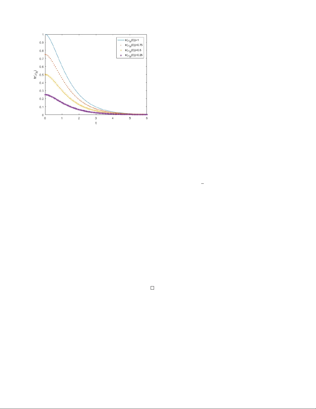
Subspace Stabilization Analysis for Non-Mark o vian Op en Quan tum Systems Shikun Zhang, 1 , ∗ Kun Liu, 1 , † Dao yi Dong, 2 Xiao xue F eng, 1 , ‡ and F eng P an 1 1 Scho ol of A utomation, Beijing Institute of T e chnolo gy, Beijing, 100081 ,China 2 Scho ol of Engine ering and Information T e chnolo gy, University of New South Wales, Caberr a, ACT, 2600, Austr alia (Dated: Decem b er 20, 2024) Studied in this article is non-Mark ovian op en quan tum systems parametrized by Hamiltonian H , coupling op erator L , and memory kernel function γ , whic h is a prop er candidate for describing the dynamics of v arious solid-state quantum information pro cessing devices. W e lo ok in to the subspace stabilization problem of the system from the p erspective of dynamical systems and con trol. The problem translates itself into finding analytic conditions that characterize inv arian t and attractiv e subspaces. Necessary and sufficient conditions are found for subspace in v ariance based on algebraic computations, and sufficien t conditions are deriv ed for subspace attractivit y by applying a double in tegral Ly apuno v functional. Mathematical pro of is given for those conditions and a numerical example is provided to illustrate the theoretical result. I. INTR ODUCTION Human beings are now in a cen tury when we can not only observe and describ e quan tum systems, but also al- ter and control them so as to harness their pow er unpar- alleled by classical resources. A promising application lies in Quan tum Information Pro cessing (QIP), where ex- p onen tially faster computation and pro v ably safer com- m unication are possible to b e realised [1]. In the recen t decade, effective QIP devices hav e b een known including silicon photonic crystals [2], trapp ed ions [3], and sup er- conducting quantum circuits [4]. “Quan tum information” in the digital w orld must b e represen ted by , stored in and manipulated through actual ph ysical systems, whose states evolv e according to the la ws of quantum mechanics and ev en quantum field the- ory . Therefore, rigorouly analysing and actively tuning the dynamics of those systems are among the fundamen- tal building blo cks of quan tum information engineering. This coincides with the basic ob jectiv e of Systems and Con trol science, whic h is to predict the evolution of dy- namical systems and make them behav e in the wa y w e desire. As a result, quan tum control (cyb ernetics) [5 – 7], b orn at the intersection of quantum ph ysics, control sci- ence and applied m athematics, b ecomes a useful tool to ac hieve successful QIP and other quantum engineering applications. In this work, w e tak e an in depth look into the subspace stabilization problem whic h lies in the realm of Systems and Control theory and finds applications in a wide range of QIP problems, e.g., initialization of qubit, generation of entangled states and realization of decoherence-free quan tum information. This problem w as first studied in [8], where it w as analysed in the framew ork of subspace in v ariance and attractivity . The authors in [8] presented ∗ daxiayusuozhang@126.com † kunliubit@bit.edu.cn ‡ fengxiaoxue@bit.edu.cn a set of algebraic conditions that c haracterize in v ariant and attractive subspaces. Moreov er, in [9], sufficient and necessary conditions were derived for in v ariance and at- tractivit y as opposed to mostly necessary conditions in the previous pap er. As subsequent works, the authors in [10] constructively designed system parameters ( H , L ) to stabilize generic quan tum states, and Ref. [11] intro- duced a computable algorithm to verify those previously prop osed conditions and analysed the sp eed of conv er- gence. Ho wev er, the subspace stabilization problem is, up to date, only cov ered for Lindblad systems [12]. Among the sev eral assumptions that lead to the Lindblad master equation lies the Mark o vian assumption, whic h requires that en vironmental correlations be sufficiently short com- pared with the system’s c haracteristic time scale. This results in a memoryless, or in other w ords, Marko vian, system where information only flo ws in one direction. Y et this assumption does not apply to all scenarios. F or in- stance, the mo delling of mesoscopic quantum circuits, where field propagation time dela y and non-classical in- put states are considered, often sees the break do wn of Mark ovian assumption [13]. It seems only natural to ex- tend the analysis of subspace stabilization in to the non- Mark ovian regime. In the recen t decade, non-Mark o vian quan tum systems ha ve attracted increasing interest from the academia. A large amount of w ork has been done on deriving prop er mathematical mo dels, defining and measuring non-Mark ovianit y , and analysing complete p ositivit y; see [14] for an excellen t review. Ho wev er, very few results ha ve addressed the prop erties of system dynamics giv en a non-Mark ovian master equation, which is a topic of ma jor fo cus for Systems and Control theorists. There- fore, we would like to study the subspace stabilization problem for non-Marko vian quan tum systems as an in- v estigation of quantum dynamics with memory and for ac hieving QIP tasks on ph ysical devices with significan t non-Mark ovian effects. The master equation on whic h our work bases w as de- riv ed in [15] for non-Mark ovian input-output netw orks. 2 It applies to atom-like structures in radiation fields, for example, the superconducting ciruit and microw a ve sys- tem. The resulting equation is a time-con volutional one where the deriv ative of current state dep ends on all his- tory states and environmen tal interactions, as opposed to its Mark o vian (Lindblad) coun terpart where only the presen t state matters. The mathematical ob ject b e- hind time con volutional non-Marko vian equations is the In tegro-Differential System, see [16], from which w e hav e tak en a page to help our discussion. The rest of the paper is organized as follows. In Sec- tion II, we in tro duce the non-Mark o vian master equation to b e studied and define the scop e of system parameters to our interest. This is follow ed b y Section I I I, where the definition of inv arian t subspaces is given and its iff con- ditions are provided and prov ed. Section IV presents the definition and sufficient conditions of subspace attrac- tivit y , and Section V gives an example of a three lev el system follo wed b y n umerical simulation. The article is concluded b y Section VI, whic h sums up the work and suggests future directions. I I. NON-MARK O VIAN SYSTEM MODEL In this article, we study non-Mark ovian open quantum systems describ ed b y the following time c on v olutional master equation, whic h was derived in [15] by applying the Born approximation. ˙ ρ = − i [ H, ρ ] + R t 0 { γ ∗ ( t − τ )[ Lρ ( τ ) , L † H ( τ − t )] + γ ( t − τ )[ L H ( τ − t ) , ρ ( τ ) L † ] } dτ , (1) where L H ( t ) = e iH t Le − iH t . (2) There are three parameters in the system mo del. The Hermitian op erator H stands for system Hamiltonian, whic h generates in ternal dynamics for the system. Mean- while, L represen ts the coupling operator, whic h de- scrib es the in teraction interface b etw een the quan tum system and its environmen t. Finally , the memory k ernel function γ ( t ) demonstrates the non-Marko vianit y of the system b y w eighing the influence of all history system- en vironment interactions. It is straigh tforw ard to v e rify that this master equation reduces to the well-kno wn and extensiv ely studied Lindblad master equation: ˙ ρ = − i [ H, ρ ] + 2 LρL † − L † Lρ − ρL † L. (3) when γ ( t ) = δ ( t ). In this scenario, memoryless kernel function leads to memoryless, or in other words, Mark o- vian, dynamics. F or the sake of simplicit y , only real k ernel functions are considered in this work. It is also assumed that γ ( t ) ≥ 0, γ (0) 6 = 0 and γ ∈ L 1 [0 , ∞ ). More restrictions on γ may need to be considered to guanrantee complete p ositivity of the non-Marko vian master equation. Ho wev er, deriv- ing suc h conditions remains a rather unexplored problem and is b eyond the scop e of this pap er. In fact, com- plete p ositivit y has b een prov en in the case of Lorentz sp ectrum quantum noises (exp onen tially decaying mem- ory k ernels) [15], whic h indicates that completely positive dynamics can be induced b y a set of k ernel functions that subsumes the exponential family . Therefore, we make a further assumption that γ b elongs to that set. Giv en that the op en system evolv es under (1), its sub- space stabilization problem is divided in to in v ariance and attractivit y analysis, which will b e discussed separately in the following sections. I II. SUBSP ACE INV ARIANCE This section in volv es the first half of subspace stabiliza- tion problem, subspace in v ariance. W e giv e a definition of inv ariant subspaces and present necessary & sufficient conditions that characterize them. Let H I b e a finite dimensional Hilbert space, and D ( H I ) b e the set of all semi-p ositiv e, trace-one, hermi- tian linear b ounded op erators on H I (densit y matrices), whic h forms the state space for quan tum system (1). The Hilb ert space admits the following decomposition, H I = H S ⊕ H R , (4) where H S = span {| ϕ S j i} m j =0 and H R = span {| ψ R k i} n k =0 . All basis v ectors are orthonormal. According to this sub- space decomp osition, each op erator in (1) has a blo ck matrix representation given this set of bases. W e denote those matrices as follows. H =  H S H P H Q H R  , L =  L S L P L Q L R  ρ ( t ) =  ρ S ( t ) ρ P ( t ) ρ Q ( t ) ρ R ( t )  , L H ( t ) =  L S H ( t ) L P H ( t ) L Q H ( t ) L R H ( t )  . The hermicit y of H and ρ implies that H Q = H † P and ρ Q ( t ) = ρ † P ( t ). W e now define what an in v arian t subspace is. It can be v erified that our definition is equiv alen t to that in [8] and [9]. Ho wev er, we simplify the narration in those works b y suppressing the notion of quan tum subsystems. Definition 1 (Subspace Inv ariance) . L et the quantum system evolve under (1). H S is an invariant subsp ac e if the fol lowing c ondition is satisfie d: if ρ (0) =  ρ 0 S 0 0 0  , ∀ ρ 0 S ∈ D ( H S ) , then ρ ( t ) =  ρ S ( t ) 0 0 0  , ∀ t ≥ 0 . 3 The follo wing theorem completely c haracterizes in v ari- an t subspaces. Theorem 1 (Subspace Inv ariance) . The fol lowing c on- ditions (i),(ii),(iii) ar e ne c essary and sufficient for H S to b e an invariant subsp ac e. (i) H =  H S 0 0 H R  ; (ii) L =  L S L P 0 L R  ; (iii) Denote by ρ S ( t ; ρ 0 S ) the tr aje ctory, with initial value ρ 0 S , which satisfies the fol lowing inte gr o-differ ential e quation. ˙ ρ S = − i [ H S , ρ S ]+ Z t 0 γ ∗ ( t − τ )[ L S ρ S ( τ ) , L S † H ( τ − t )] + h.c. dτ , (5) wher e L S H ( t ) = e iH S t L S e − iH S t . (6) Then, ∀ ρ 0 S ∈ D ( H S ) , Z t 0 γ ( t − τ ) ρ S ( τ ; ρ 0 S ) L † S L P H ( τ − t ) dτ = 0 . (7) Pr o of. Necessit y . Supp ose H S is an in v ariant subspace, then w e ha ve the follo wing relationship according to Definition 1: ρ ( t ) =  ρ S ( t ; ρ 0 S ) 0 0 0  , ∀ t ≥ 0 , ∀ ρ 0 S ∈ D ( H S ); ˙ ρ ( t ) =  ˙ ρ S ( t ; ρ 0 S ) 0 0 0  =  S ( t ) P ( t ) Q ( t ) R ( t )  , ∀ t ≥ 0 . Hermitit y of the state densit y matrix and its deriv ative imply that Q ( t ) = P † ( t ). W e pro ceed to compute explic- itly the S, P and R blo cks. S ( t ) = − i [ H S , ρ S ] + Z t 0 { γ ∗ ( t − τ )[ L S ρ S ( τ ) , L S † H ( τ − t )] − L Q † H ( τ − t ) L Q ρ S ( τ ) } + h.c. dτ , (8) P ( t ) = iρ S H P + Z t 0 γ ∗ ( t − τ ) L S ρ S ( τ ) L Q † H ( τ − t ) + γ ( t − τ )[ L S H ( τ − t ) ρ S ( τ ) L † Q − ρ S ( τ )( L † S L P H ( τ − t ) + L † Q L R H ( τ − t ))] dτ , (9) R ( t ) = Z t 0 γ ∗ ( t − τ ) L Q ρ S ( τ ) L Q † H ( τ − t ) + h.c. dτ . (10) Since R ( t ) ≡ 0, then ˙ R ( t ) ≡ 0, and ˙ R (0) = 0. Changing the integration v ariable yields: R ( t ) = Z t 0 γ ∗ ( τ ) L Q ρ S ( t − τ ) L Q H ( − τ ) + h.c. dτ , (11) ˙ R ( t ) = Z t 0 γ ∗ ( τ ) L Q ∂ t ρ S ( t − τ ) L Q H ( − τ ) + h.c. dτ + γ ∗ ( t ) L Q ρ 0 S L Q † H ( − t ) + h.c. , (12) ˙ R (0) = ( γ ∗ (0) + γ (0)) L Q ρ 0 S L † Q = 0 , ∀ ρ 0 S ∈ D ( H S ) . (13) Therefore, L Q = 0. The S and P blo c ks are thus reduced to: S ( t ) = − i [ H S , ρ S ] + Z t 0 γ ∗ ( t − τ )[ L S ρ S ( τ ) , L S † H ( τ − t )] + h.c. dτ , (14) P ( t ) = iρ S H P + Z t 0 γ ∗ ( t − τ ) L S ρ S ( τ ) L Q † H ( τ − t ) − γ ( t − τ ) ρ S ( τ ) L † S L P H ( τ − t ) dτ . (15) Moreo ver, since P (0) = iρ 0 S H P = 0, the arbitrariness of ρ 0 S indicates that H P = 0. It follo ws that H m ust ha ve a blo c k diagonal structure, thus leading to the explicit form of L H ( t ): L H ( t ) =  e iH S t L S e − iH S t e iH S t L P e − iH R t 0 e iH R t L R e − iH R t  . (16) This structure implies that L Q H ( t ) = 0, which further reduces the P blo c k to: P ( t ) = − Z t 0 γ ( t − τ ) ρ S ( τ , ρ 0 S ) L † S L P H ( τ − t ) dτ ≡ 0 . (17) Necessit y is thus prov ed. Sufficiency . Supp ose that conditions (i) , (ii) and (iii) are satis- fied. Direct computation yields the follo wing integro- differen tial equations for sub-blo c ks of the state densit y matrix: ˙ ρ S ( t ) = − i [ H S , ρ S ] + Z t 0 γ ∗ ( t − τ ) { [ L S ρ S ( τ ) + L P ρ † P ( τ ) , L S † H ( τ − t )] + ( L S ρ P ( τ ) + L P ρ R ( τ )) L P † H ( τ − t ) } + h.c. dτ , (18) 4 ˙ ρ P ( t ) = − i ( H S ρ P − ρ P H R ) + Z t 0 γ ∗ ( t − τ )[( L S ρ P ( τ ) + L P ρ R ( τ )) L R † H ( τ − t ) − L S † H ( τ − t )( L S ρ P ( τ ) + L P ρ R ( τ ))] + γ ( t − τ )[( L S H ( τ − t ) ρ P ( τ ) + L P H ( τ − t ) ρ R ( τ )) L † R − ( ρ S ( τ ) L † S + ρ R ( τ ) L † P ) L P H ( τ − t ) − ρ R ( τ ) L † R L R H ( τ − t )] dτ , (19) ˙ ρ R ( t ) = − i [ H R , ρ R ] + Z t 0 γ ∗ ( t − τ ) { [ L R ρ R ( τ ) , L R † H ( τ − t )] − L P † H ( τ − t )( L S ρ P ( τ ) + L P ρ R ( τ )) } + h.c. dτ . (20) It suffices to v erify that ρ ( t ; ρ 0 S ), ρ P ( t ) ≡ 0, and ρ R ( t ) ≡ 0 are solutions of (18), (19), and (20). It is clear that (18) and (20) are satisfied, while (19) leads to: − Z t 0 γ ( t − τ ) ρ S ( τ ; ρ 0 S ) L † S L P H ( τ − t ) dτ = 0 (21) whic h is satisfied because of condition (iii) . This com- pletes the pro of of sufficiency . Although the conditions given in Theorem 1 are nec- essary and sufficient, condition (iii) may b e difficult to v erify for systems with high dimensions. Therefore, some useful necessary (not sufficient) and sufficien t (not nec- essary) conditions are provided. Corollary 1. Consider the fol lowing c onditions (iv) and (v): (iv) L † S L P = 0 ; (v) [ L † S , H S ] = 0 . (iv) is ne c essary for H S to b e invariant. (i), (ii), (iv) and (v) ar e sufficient for subsp ac e invarianc e. Pr o of. W e b egin by showing that (iv) is necessary . Calculating the deriv ativ e of P ( t ) at t = 0 yields: ˙ P (0) = − γ (0) ρ 0 S L † S L P = 0 , whic h holds for arbitrary ρ 0 S . This implies that L † S L P = 0. F or the sufficiency of (i) , (ii) , (iv) and (v) , w e prov e that (iv) and (v) leads to (iii) . This is clear since: L † S L P H ( τ − t ) = L † S e iH S ( τ − t ) L P e − iH S ( τ − t ) = e iH S ( τ − t ) L † S L P e − iH S ( τ − t ) = 0 . Th us ends the pro of of Corollary 1. After defining and c haracterizing in v ariant subspaces, it can be seen that each of them determines an “inv ari- an t set” in D ( H I ), whic h is the set of density matrices that are ”compressed” within the top left S blo ck. If the initial state lo cates in that set, all future states will remain in it as long as the system ev olves under (1). In- v ariant subspaces thus correspond to preserved quantum information. Moreov er, they pav e the wa y for subspace attractivit y , which will b e discussed in the next section. IV. SUBSP ACE A TTRA CTIVITY Building on the analysis of subspace in v ariance in the previous section, we pro ceed to define and characterize attractiv e subspaces. It can also b e c hec ked that this is equiv alent to the definition in [8]. Definition 2 (Subspace Attractivit y) . L et ρ ( t ) evolve under (1). If lim t → + ∞ ( ρ ( t ) −  ρ S ( t ) 0 0 0  ) = 0 for al l initial states in D ( H I ) , and H S is invariant, then H S is said to b e an attr active subsp ac e. It is straigh tforward from this definition that an attrac- tiv e subspace H S is related to an in v ariant and attractiv e set of density matrices. Supp ose [ L † S , H S ] = 0. Then (20) reduces to the fol- lo wing equation considering real γ functions. ˙ ρ R ( t ) = − i [ H R , ρ R ] + Z t 0 γ ( t − τ ) { [ L R ρ R ( τ ) , L R † H ( τ − t )] + [ L R H ( τ − t ) , ρ R ( τ ) L † R ] } dτ + Z t 0 γ ( t − τ )( − L P † H ( τ − t ) L P ρ R ( τ ) − ρ R ( τ ) L † P L P H ( τ − t )) dτ . (22) This implies that the evolution of ρ R is independent, as opp osed to (20), where it also relies on ρ P . W e cast (22) into superop erator form: ˙ ρ R = A ρ R + Z t 0 B ( t − τ ) ρ R ( τ ) dτ + Z t 0 K ( t − τ ) ρ R ( τ ) dτ , (23) where A [ · ] = − i [ H R , · ] , B ( t )[ · ] = γ ( t ) { [ L R · , L R † H ( − t )] + [ L R H ( − t ) , · L † R ] } , K ( t )[ · ] = − γ ( t )( L P † H ( − t ) L P · + · L † P L P H ( − t )) . Before presen ting the main theorem of this section, we shall first prov e a useful lemma. 5 Lemma 1. L et f ( t ) b e a c ontinuously differ entiable func- tion on [0 , ∞ ) , and f ( t ) ≥ 0 . If ˙ f ( t ) ≤ φ ( t ) , wher e φ ( t ) ≥ 0 and φ ∈ L 1 [0 , ∞ ) , then f ( t ) must have a finite limit when t tends to infinity. Pr o of. W e first pro ve that the statemen t is correct when ˙ f ( t ) has a finite num b er of zero p oin ts. Let t max b e the largest zero p oin t. On ( t max , ∞ ), ˙ f ( t ) m ust either remain negative or p ositive. If it remains negativ e, then f ( t ) m ust hav e a limit since it is descend- ing and low er bounded b y 0 on ( t max , ∞ ). If it remains p ositiv e, consider the following inequalities. f ( t ) = f (0) + R t 0 ˙ f ( s ) ds ≤ f (0) + R t 0 φ ( s ) ds ≤ f (0) + R ∞ 0 φ ( s ) ds. Because φ ∈ L 1 [0 , ∞ ), f ( t ) is upper b ounded. It th us has a limit since it is increasing on ( t max , ∞ ). W e then pro ceed to consider the case where ˙ f ( t ) has an infinite n umber of zero p oints. The statemen t can b e pro ved b y con tradiction. Supp ose that f ( t ) has no limits. Then we hav e: U = lim t → + ∞ f ( t ) > lim t → + ∞ f ( t ) = L. Denote the sequence of p eaks b y { u n } ∞ n =1 , and the se- quence of v alleys by { l n } ∞ n =1 . The definition of limit su- p erior and limit inferior implies that: U = lim t → + ∞ f ( t ) = lim n → + ∞ u n , L = lim t → + ∞ f ( t ) = lim n → + ∞ l n . The equiv alent definition of sup erior and inferior limits indicates that there exist { u n k } ∞ k =1 ⊂ { u n } ∞ n =1 , lim k → + ∞ u n k = U ; { l n k } ∞ k =1 ⊂ { l n } ∞ n =1 , lim k → + ∞ l n k = L. W e also hav e that ∀ t, s > 0, t ≥ s , f ( t ) − f ( s ) = Z t s ˙ f ( τ ) dτ ≤ Z t s φ ( τ ) dτ . Since φ ∈ L 1 [0 , ∞ ), f ( t ) − f ( s ) tends to 0 when t and s tend to infinit y . How ever, if w e pic k { u n k i } ∞ i =1 ⊂ { u n k } ∞ k =1 , s.t. l n i ≤ u n k i , ∀ i ∈ N + , we hav e: lim i → + ∞ ( f ( u n k i ) − f ( l n i )) = U − L > 0 . This results in a con tradiction. Therefore, f ( t ) m ust ha v e a limit. W e are no w in the position to presen t the main result on subspace attractivity . Theorem 2 (Subspace Attractivit y) . If [ L † S , H S ] = 0 , and the matrix − 2 γ (0) L † P L P + Z ∞ t k Ω( τ , t ) k dτ · I is ne gative definite for al l t ≥ 0 , then H S is an attr active subsp ac e. Ω( · , · ) is a two-variable sup er op er ator expr esse d as: Ω( t, s ) = K ( t − s ) − ∂ s K ( t − s ) − K ( t − s ) A − Z t s K ( t − u )( K ( u − s ) + B ( u − s )) du. (24) Pr o of. Since ρ ( t ) is alwa ys positive, it suffices to sho w that the origin is asymptotically stable (all solutions tend to 0) for (22) and (23). The V ariation of Parameters tec hnique of integro-differen tial equations; see [16], allo w us to swap (23) into an equiv alen t equation: ˙ σ = N σ + Z t 0 L ( t, s ) σ ( s ) ds + K ( t ) σ 0 , (25) where N = A − K (0) , and L = Ω( t, s ) + B ( t, s ) . Consider the following Lyapuno v functional: V ( t, σ ( · )) = tr ( σ ) + Z t 0 Z ∞ t k Ω( τ , s ) k dτ tr ( σ ( s )) ds, (26) where k · k denotes the norm of superop erators on the Ba- nac h space of all Hermitian matrices. T aking the deriv a- tiv e of this functional w.r.t t yields: ˙ V ( t, σ ( · )) = tr(( A − K (0)) σ ) + tr( Z t 0 (Ω)( t, s ) σ ( s ) ds ) + tr( Z t 0 ( B )( t, s ) σ ( s ) ds ) + tr( K ( t ) σ 0 ) − Z t 0 k Ω( t, s ) k tr( σ ( s )) ds + Z ∞ t k Ω( τ , t ) k dτ tr( σ ) . (27) Using the fact that tr( A [ · ]) = 0 and tr( B ( t, s )[ · ]) = 0, and applying the norm inequality we obtain: ˙ V ( t, σ ( · )) ≤ − tr( K (0) σ ) + tr( Z t 0 k Ω( t, s ) k σ ( s ) ds ) + tr( K ( t ) σ 0 ) − Z t 0 k Ω( t, s ) k tr( σ ( s )) ds + Z ∞ t k Ω( τ , t ) k dτ tr( σ ) = tr([ − 2 γ (0) L † P L P + Z ∞ t k Ω( τ , t ) k dτ · I ] σ )+tr( K ( t ) σ 0 ) . 6 FIG. 1. F our differen t initial v alues for tr( ρ R ): 1, 0.75, 0.5, 0.25 are chosen. Simulation results show that tr( ρ R ) v anishes as time elapses, demonstrating subspace attractivity . The negative definiteness of − 2 γ (0) L † P L P + Z ∞ t k Ω( τ , t ) k dτ · I implies that ˙ V ( t, σ ( · )) ≤ tr( K ( t ) σ 0 ), which is a scalar function in L 1 [0 , ∞ ) because γ ∈ L 1 [0 , ∞ ) and all other time dep enden t terms are oscillatory and b ounded. Therefore, by applying Lemma 1, we know that the Ly apunov functional (26) must ha ve a finite limit when t tends to infinit y . The natural b oundedness of densit y matrices implies that the second deriv ative of V w.r.t t is also b ounded. The Barbalat’s lemma thus tells us that ˙ V tends to zero. This leads to the fact that lim t → + ∞ tr([ − 2 γ (0) L † P L P + Z ∞ t k Ω( τ , t ) k dτ · I ] σ ) = 0 b ecause tr( K ( t ) σ 0 ) tends to 0. The negativ e definiteness again says that σ ( t ) → 0, which completes the pro of. Remark 1. In an attr active subsp ac e, the invariant set determine d by the subsp ac e is autonomously stabilize d for al l initial states. This is inter esting for QIP applic ations, wher e quantum information may b e manipulate d and fr e e fr om de c oher enc e. If the attr active subsp ac e is only one- dimensional, then the set shrinks to a single pur e state that sp ans the subsp ac e. T asks such as qubit initializa- tion, c o oling and entanglement gener ation c an b e r e alize d if we cho ose a pr op er subsp ac e de c omp osition. V. NUMERICAL EXAMPLE AND SIMULA TION In this section, an example with n umerical simulation is presented to illustrate the results. Consider a three-level system with the following pa- rameters, where we ha ve set ¯ h = 1. The k ernel function is γ ( t ) = e − 3 t and H =   1 / 2 0 0 0 − 1 / 2 0 0 0 − 1 / 2   , L =   1 0 0 0 0 1 0 0 0   . The S blo ck corresp onds to the 2 × 2 blo ck on the top left. The corresponding subspace H S is thus 2- dimensional. Its attractivity will b e demonstrated via sim ulation. It can b e verified directly that the matri- ces satisfy sufficien t conditions for inv ariance proposed in Section I I I. Direct computation yields: − 2 γ (0) L † P L P + Z ∞ t k Ω( τ , t ) k dτ ≤ − 2 + Z ∞ 0 e − 3 u | 4 − 4 u | du ≤ − 2 9 < 0 . Therefore, sufficient conditions for attractivit y are also met. W e plot tr( ρ R ) w.r.t time in FIG.1, c ho osing 4 differen t initial v alues. FIG.1 sho ws that they conv erge to 0, meaning that H S is attractive. VI. CONCLUSION AND FUTURE W ORK W e ha ve extended the analysis of subspace inv ariance and attractivit y to a class of non-Marko vian quantum systems. By doing so, we attempt to reac h deeper than only to mo del non-Marko vian systems: w e ha v e also set fo ot on inv estigating their asymptotic dynamical prop er- ties, which is among the first few attempts in literature to our knowledge. In future works, other non-Mark ovian mo dels with potential QIP applications will b e in vesti- gated. It is also w orth while in v estigating whether non- Mark ovian quantum systems may hav e other undefined dynamical prop erties compared with their Marko vian coun terpart, which only mak es future studies muc h more in triguing. A CKNOWLEDGMENTS This w ork has b een supp orted b y National Natu- ral Science F oundation (NNSF) of China under Grant 61603040. 7 [1] M. A. Nielsen and I. L. Chuang, Quantum Computa- tion and Quantum Information, 10th A nniversary Edi- tion (Cambridge Universit y Press, 2010) pp. 1–59. [2] A. H. Atabaki, S. Moazeni, F. Pa v anello, H. Gevorgy an, J. Notaros, L. Alloatti, M. T. W ade, C. Sun, S. A. Kruger, and H. Meng, Nature 556 (2018). [3] M. Bo c k, P . Eich, S. Kucera, M. Kreis, A. Lenhard, C. Becher, and J. Eschner, Nature Communications 9 (2018). [4] S. S., M. Hatridge, Z. Leghtas, S. K. M, N. A., V. U., G. S. M, F. L., M. M., and D. M. H, Nature 504 , 419 (2013). [5] D. Dong and I. R. Petersen, Control Theory and Appli- cations IET 4 , 2651 (2010). [6] C. Altafini and F. Ticozzi, IEEE T ransactions on Auto- matic Control 57 , 1898 (2012). [7] J. Zhang, Y.-X. Liu, R. B. W u, K. Jacobs, and F. Nori, Ph ysics Rep orts 679 (2017). [8] F. Ticozzi and L. Viola, IEEE T ransactions on Automatic Con trol 53 , 2048 (2008). [9] F. Ticozzi and L. Viola, Automatica 45 , 2002 (2009). [10] F. Ticozzi, S. G. Sc hirmer, and X. W ang, IEEE T rans- actions on Automatic Con trol 55 , 2901 (2010). [11] F. Ticozzi, R. Lucchese, P . Capp ellaro, and L. Vi- ola, IEEE T ransactions on Automatic Control 57 , 1931 (2012). [12] H. P . Breuer and F. Petruccione, The The ory of Op en Quantum Systems (Oxford Universit y Press,, 2002) pp. xxii,625. [13] J. Combes, J. Kerc khoff, and M. Sarov ar, Adv ances in Ph ysics X 2 (2016). [14] I. D. V ega and D. Alonso, Rev. Mo d. Phys 89 (2017). [15] J. Zhang, Y. Liu, R. B. W u, K. Jacobs, and F. Nori, Ph ysical Review A 87 , 1 (2013). [16] V. Lakshmik antham, The ory of Inte gr o-Differ ential Equations , Stability and Con trol (CRC Press, 1995). [17] A. Shabani and D. A. Lidar, Physical Review A 71 , 159 (2005). [18] P . P ech uk as, Ph ysical Review Letters 73 , 1060 (1994). [19] Y. Pan and T. Nguy en, IEEE T ransactions on Automatic Con trol , 1 (2016). [20] B. V acc hini, Ph ysical Review Letters 117 , 230401 (2016). [21] S. B. Xue, R. B. W u, W. M. Zhang, J. Zhang, C. W. Li, and T. J. T arn, Physical Review A 86 , 10870 (2012). [22] B. V acc hini, Physical Review A 87 , 184 (2013).