Statistical inference of probabilistic origin-destination demand using day-to-day traffic data

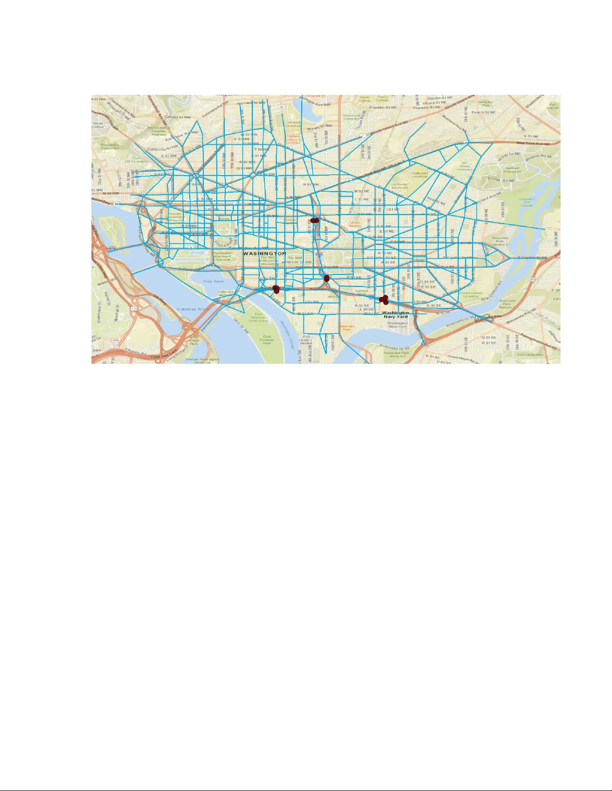
Statistical inference of probabilistic origin-destination demand using day-to-day traf ﬁc data W ei Ma, Zhen (Sean) Qian Department of Ci vil and En vironmental Engineering Carnegie Mellon Uni versity , Pittsb urgh, P A 15213 { weima, seanqian } @cmu.edu December 20, 2024 Abstract Recent transportation network studies on uncertainty and reliability call for modeling the probabilis- tic O-D demand and probabilistic network ﬂow . Making the best use of day-to-day trafﬁc data collected ov er many years, this paper dev elops a novel theoretical framework for estimating the mean and vari- ance/cov ariance matrix of O-D demand considering the day-to-day variation induced by travelers’ inde- pendent route choices. It also estimates the probability distrib utions of link/path ﬂo w and their trav el cost where the variance stems from three sources, O-D demand, route choice and unknown errors. The frame- work estimates O-D demand mean and v ariance/covariance matrix iterati vely , also kno wn as iterati ve gen- eralized least squares (IGLS) in statistics. Lasso regularization is employed to obtain sparse cov ariance matrix for better interpretation and computational efﬁcienc y . Though the probabilistic O-D estimation (ODE) w orks with a much larger solution space than the deterministic ODE, we sho w that its estimator for O-D demand mean is no worse than the best possible estimator by an error that reduces with the increase in sample size. The probabilistic ODE is e xamined on two small networks and two real-world lar ge-scale networks. The solution con v erges quickly under the IGLS frame work. In all those e xperiments, the results of the probabilistic ODE are compelling, satisfactory and computationally plausible. Lasso regularization on the co variance matrix estimation leans to underestimate most of variance/co variance entries. A proper Lasso penalty ensures a good trade-off between bias and v ariance of the estimation. 1 Intr oduction Origin-destination (O-D) demand is a critical input to system modeling in transportation planning, operation and management. For decades, O-D demand is deterministically modeled, along with deterministic mod- els of link/path ﬂow and travel cost/time in classical traf ﬁc assignment problems. T ransportation network uncertainty and reliability call for modeling the stochasticity of O-D demand, namely its spatio-temporal correlation and variation. W ith the increasing quantity and quality of trafﬁc data collected years along, it is possible to learn the stochasticity of O-D demand for better understanding stochastic travel behavior and stochastic system performance metrics. Some studies considered the stochastic features of O-D demand, b ut few estimated the mean and v ariance of O-D demand from day-to-day traf ﬁc data. What is missing in the lit- erature is the capacity to estimate spatially correlated multiv ariate O-D demand, in conjunction with a sound network ﬂow theory on probabilistic route choices that can be learned from day-to-day trafﬁc data. In view 1 of this, this paper de velops a novel data-friendly framework for estimating the mean and variance/cov ariance of O-D demand based on a generalized statistical network equilibrium. The statistical properties to wards the estimated probabilistic O-D demand are also analyzed and pro vided. The process of O-D demand estimation (ODE) is further examined in real-world netw orks for insights. O-D estimation (ODE) requires an underlying behavioral model, based on which O-D demand is es- timated such that it best ﬁts observations. Behavioral models in the static network context, namely route choice models, are also known as static trafﬁc assignment models. The classical trafﬁc assignment mod- els [e.g., 20 , 63 ] deterministically map the deterministic O-D demand q ∈ R R × S + to link ﬂo w x ∈ R N + or path ﬂo w f ∈ R K + (where R , S , N and K are the cardinality of sets of origins, destinations, links, and paths, respecti vely). In fact, the deterministic O-D demand q is assumed to represent the mean number of vehicles in the same peak hour from day to day . Lik ewise, link (path) ﬂo w is also deterministic, represent- ing the mean number of vehicles on a link (path) in the same hour from day to day . The classical trafﬁc assignment models (such as User Equilibrium and Stochastic User Equilibrium) lay out the foundation of deterministic O-D estimation methods, namely to estimate q in a way to best ﬁt observed data related to a subset of link/path ﬂow x, f . Deterministic O-D estimation (ODE) include the entropy maximizing models [ 80 ], maximum likelihood models [ 75 , 87 ], generalized least squares (GLS) models [ 9 , 5 , 93 , 84 ], Bayesian inference models [ 49 , 76 ] and some recent emerging combined models [ 2 , 14 , 43 , 15 , 45 , 90 ]. F or more details, readers are referred to the comprehensiv e revie ws by Bera and Rao [ 6 ], Castillo et al. [ 11 ]. Classical trafﬁc assignment models and ODE methods overlook the variance/co variance of demand and link/path ﬂow , an essential feature for network trafﬁc ﬂo w . Recent studies on network reliability and un- certainty model stochasticity of the network ﬂow . Since ODE requires a traf ﬁc assignment model, we ﬁrst revie w statistical traf ﬁc assignment models, followed by ODE models that take into account stochasticity . One aspect of the stochastic network ﬂo w is using probability distributions to represent O-D demand. For e xample, W aller et al. [ 83 ], Duthie et al. [ 24 ] sampled O-D demand from giv en multi variate normal dis- tributions (MVN) and e v aluated the network performance under classical User Equilibrium (UE) condition. Chen et al. [ 17 ] used a similar simulation-based method to ev aluate trav elers’ risk-taking behavior due to probabilistic O-D demand. All these studies indicate the O-D variation is of great importance to network modeling and behavioral analysis. Statistical trafﬁc assignment models consider various O-D probability distributions such as Poisson distributions [ 19 ], MVN [ 13 ], multinomial distributions [ 51 ]. Nakayama and W atling [ 54 ] summarized different formulations and proposed a uniﬁed framework for stochastic modeling of trafﬁc ﬂows. Advantages and disadvantages of modeling trafﬁc with those probabilistic distributions are also discussed by Castillo et al. [ 16 ]. Shao et al. [ 69 , 70 ] proposed a reliability-based trafﬁc assignment model (R UE) and extended it to consider different trav elers’ risk taking behavior . Lam et al. [ 40 ] further extended the model to consider the trafﬁc uncertainty and proposed reliability-based statistical trafﬁc equi- librium. Zhou and Chen [ 99 ], Chen and Zhou [ 18 ] proposed a α -reliable mean-excess trafﬁc assignment model which e xplicitly models the tra vel time distrib ution and consider the reliability and uncertainty of the trav el time on travelers’ route choice behavior . Other studies [ 30 , 82 , 24 ] show that the variance/co variance matrix of the O-D demand hav e a signiﬁcant inﬂuence on network traf ﬁc conditions. Though adopting stochastic O-D demand, those traf ﬁc assignment models (except Clark and W atling [ 19 ]) assumed non-atomic (inﬁnitesimal) players and therefore are unable to capture the stochasticity of route choices that vary from day to day (the proof is sho wn in Ma and Qian [ 48 ]). Classical UE, SUE and RUE are all deterministic route choice models where the number of (inﬁnitesimal) players assigned to each route is ﬁxed, rather than being stochastic. Thus, those models are unable to explain the day-to- day variation of observed trafﬁc counts at the same location and the same time of day . T o further see ho w classical equilibrium models o verlook the route choice stochasticity , suppose there is Q tra velers where Q is a random variable to be realized on each day . Giv en the probability of choosing a route p , the route ﬂow 2 is deterministically identiﬁed by the number of inﬁnitesimal users who take this route, F = pQ . Even if the route choice probability p is determined by stochastic choice models (such as Probit, Logit, etc.), these models still assume that a ﬁxed number Qp of trav elers take this route on each day , as a result of non-atomic equilibrium. This does not, theoretically , allow to model the day-to-day v ariations of trav elers’ choices. Recent studies on statistical traf ﬁc assignment models indicate that the route ﬂow is the aggregation of random choices of O-D demand, and thus also random [ 85 , 86 , 52 , 53 , 54 ]. T ravelers’ route choice follows a multinomial distrib ution with the probability obtained from route choice models, f ∼ Multinomial ( Q, p ) . T o distinguish to what extent stochasticity is modeled for route choices, we refer to the former (classical) models as “ ﬁxed portions with stochastic r oute choice models ” and the latter models as “ probabilistic distrib utions with stochastic r oute choice models ”. Though route choices are stochastic, these studies did not work directly with the co variance of demand among all O-D pairs. A detailed comparison of those assignment models is further illustrated in Ma and Qian [ 48 ]. Giv en a route choice probability , we can deri ve probability distributions of path/link ﬂow . Howe ver , it is non-trivial to establish a statistical network equilibrium where the route choice probability is determined en- dogenously as a result of stochastic O-D demand, path/link ﬂow and netw ork conditions. In the deterministic settings, UE, SUE or R UE simultaneously determines the mean path/link ﬂow , and the route choice probabil- ity [e.g., 93 ]. V ery few studies e xamined the statistical network equilibrium. Davis and Nihan [ 22 ] proposed a Marko v process to model the day-to-day v ariation of trafﬁc ﬂow gi ven a ﬁx ed regional population. The stochastic route choice on a particular day is assumed to be related to the stochastic netw ork condition of the previous days [ 10 ]. When the network e volv es from day to day , there exists a netw ork equilibrium where stabilized probability distrib utions of path/link ﬂow are reached. Different from this approach, Ma and Qian [ 48 ] proposed a generalized statistical equilibrium where each traveler makes stochastic choices based on his/her entire past experience, namely the probability distrib utions of the equilibrated network conditions. Ma and Qian [ 48 ] inte grates multi variate probability distrib utions of O-D demands and link/path ﬂo w into the stochastic route choice models, and ultimately solved for the probabilistic network ﬂow . It also ana- lytically decomposes the v ariance of link/path ﬂow into three sources, O-D demand variation, route choice variation and measurement error . W ith little w ork on statistical traf ﬁc assignment models, probabilistic ODE can be challenging. An ideal probabilistic ODE should posses three critical features: estimating v ariance/cov ariance of O-D demand in addition to its mean, a statistical network equilibrium that can ﬁt massi ve data collected years along, and consideration of day-to-day route choice v ariation. T o our best knowledge, few literature works with ODE models that take into account any of the three features. W e summarize existing representative ODE models in Figure 1 . T o further distinguish our work from existing literature, V ardi [ 81 ], Hazelton [ 31 , 32 , 33 ], Li [ 42 ], Parry and Hazelton [ 61 ] assumed O-D demand follows Poisson distributions that are independent among O-D pairs, and Hazelton [ 31 , 32 , 33 ], Li [ 42 ], Parry and Hazelton [ 61 ] further considered day-to-day route choice variation. They formulated maximum likelihood estimator and Bayesian inference method for O-D demand, whereas the demand cov ariance among O-D pairs is not considered. In addition, using uncongested networks simpliﬁes the route choice model, and thus no network equilibrium under congestion is proposed. Shao et al. [ 67 ], Y ang et al. [ 95 ] proposed a generalized model to estimate the mean and variance of O-D demand with MVN. Shao et al. [ 68 ] further extended the model to estimate multi-class O-D demand and used L 1 regularizer to shrink the model dimensions. An equilibrium is used to model deterministic route choices (similar to classical UE and R UE), while neither of them considered day-to-day route choice variation. T o our best kno wledge, there is a lack of study that estimates correlated multiv ariate probabilistic O-D demand under a mathematically sound statistical network equilibrium (namely a truly stochastic route choice model) while considering day-to-day random route choices simultaneously . T o ﬁll up this gap, this paper 3 V a ri a nce/ co v a ri a n ce o f O - D dem a nd D a y - to - da y R o ute C ho i ce V a ri a ti o n Sta ti s ti ca l Equil i bri um Ma he r (1983 ) S ha o e t a l. (2014 ) Shao e t a l. ( 2015 ) Y a ng e t a l. (1992) This pape r This pape r Ha z e lt on, M.L . (2000 , 2001b) None L i (2005 ) Figure 1: O-D estimation methods by categories builds an ODE model based on the generalized statistical trafﬁc assignment model (GEST A) proposed by Ma and Qian [ 48 ]. Any observ ation (such as link/path ﬂow , or trav el time/cost) has a variance that stems from three sources, O-D demand variation, route choice v ariation and unkno wn errors, all from day to day . Using GEST A as the underlying behavioral model, we estimate probability distributions of O-D demand using data from v arious data sources. Furthermore, con ventional goodness-of-ﬁt indicators [e.g., 1 ] is not suitable for probabilistic ODE. This paper also proposes new goodness-of-ﬁt indicators based on probability distributions to e v aluate the performance of probabilistic ODE. Another important issue for ODE is the observ ability problem [ 12 , 94 ]. It is well kno wn that the ODE is underdetermined using observed link-based trafﬁc counts [ 93 ]. Hazelton [ 34 ] suggested to use second-order statistical information of the observed link counts to estimate Poisson distributed O-D demand without co- variance among O-D pairs. By utilizing the second-order information, the Poisson distributed O-D demand can be estimated uniquely . Y ang and Fan [ 94 ] proposed to uniquely determine the O-D demand by properly selecting data among observed link ﬂo w data and historical O-D information. Y ang et al. [ 95 ] also sho wed that possibly dissimilar multi-day observ ation improv es the observability of OD demand [ 95 ]. Hazelton et al. [ 35 ] proposed new method for sampling latent route ﬂows conditional on the observed link counts when the networks link-path incidence matrix is unimodular . In this paper , the observ ability of the proposed probabilistic ODE is examined. The new ODE guarantees that its estimator for the O-D demand mean is no worse than the con ventional deterministic ODE by the order of O ( 1 n ) , provided with suf ﬁcient data. Under the proposed probabilistic ODE frame work, we propose to estimate the O-D demand mean and variance-co variance matrix iteratively , which decomposes the complex ODE into two sub-problems. In the sub-problem of estimating O-D demand mean vector q , we extend the statistical ODE from Menon et al. [ 50 ], and both single lev el and bi-level ODE formulations are discussed. In the sub-problem of estimating O-D demand variance-cov ariance matrix Σ q , we utilize estimated link ﬂo w cov ariance to formulate the estimation problem, and then apply Lasso regularization and conv ex relaxation on the formulation. How to use trafﬁc speed data in addition to trafﬁ c counts data is discussed. Furthermore, the statistical properties of the estimated probabilistic O-D demand are provided for insights. The observability of the ODE problem is 4 also examined. The main contributions of this paper are summarized as follo ws: 1) It proposes a nov el theoretical framework for estimating probabilistic O-D demand (namely mean and variance/co variance of O-D demand) considering newly deﬁned generalized statistical network equi- librium. The statistical equilibrium simultaneously integrates probabilistic O-D demand and trav elers’ day-to-day route choice variation. 2) It deﬁnes the goodness-of-ﬁt for probabilistic ODE and develops a theory for variance analysis of estimated probabilistic O-D demand and path/link ﬂow . 3) It discusses the observability issue for probabilistic O-D demand, and shows that the estimated mean of O-D demand using the the probabilistic ODE is no worse than the estimate O-D demand using a deterministic ODE model, provided with suf ﬁcient data. 4) It intensi vely examines the proposed probabilistic ODE frame work on two lar ge-scale real networks using both simulated trafﬁc data and real world trafﬁc counts to gain insights from solutions, as well as to show the computational ef ﬁciency of the solution algorithms. The remainder of this paper is org anized as follo ws. Section 2 presents an illustrative example to further explain how and why it is necessary to consider day-to-day route choice variation. Section 3 discusses the formulation details, followed by section 4 presenting properties of the model and addressing the observability issues. Section 5 proposes the entire probabilistic ODE framework. In section 6 , two simple illustrative examples are used to demonstrate the concepts and ODE results. T wo large scale networks are used to demonstrate the computational efﬁcienc y of the probabilistic ODE method, and its ability to work with real-world data. Finally , conclusions are drawn in section 7 . 2 An illustrativ e example Observations of link/path ﬂow varies from day to day . In principle, the day-to-day variation is attributed to three sources, O-D demand variation, route choice variation and sensing measurement error . The impact of day-to-day O-D demand v ariation and measurement error on link/path ﬂo w hav e been thoroughly discussed by Y ang et al. [ 93 ], W aller et al. [ 82 ], Shao et al. [ 67 ]. Here we use a toy example to compare probabilistic O- D estimation results with and without the consideration of day-to-day route choice variation. It is intended to illustrate that where the day-to-day route choice v ariation comes from, and why it is important to not ne glect it when estimating O-D demand. Consider a toy network as shown in Figure 2 , on each day Q amount of vehicles depart from node r to node s . W e assume Q is normally distributed, so is the link ﬂow (i.e. path ﬂow in this example) X 1 and X 2 , the number of vehicles on link 1 and link 2, respectiv ely . Suppose both links are indifferent. W e do not consider measurement error here. On each day , the demand Q is realized, b ut cannot be directly measured. Instead, we measure the link ﬂow X 1 on each day . Suppose after observ ations of many days, we determine the probability distrib ution of X 1 ∼ N (50 , 10 2 ) . If we do not consider the day-to-day route choice v ariation, the estimated O-D demand follows the rounded normal distrib ution Q = [ Q 0 ] , Q 0 ∼ N (100 , 20 2 ) since Q ' 2 X 1 by equilibrium conditions. In fact, regardless of which route choice models (logit, probit, etc.), the distribution of the O-D demand can be directly computed since both links are indif ferent to tra velers. Both links hav e the same ﬂow distributions. 5 r s L i nk 1 L i nk 2 Figure 2: A toy network Now consider travelers’ route choice that v aries from day to day . The probability of an y vehicle choosing link 1 and link 2 is p 1 = p 2 = 0 . 5 . All Q v ehicles make this choice independently on each day . Thus, the link ﬂow follo ws a multinomial distribution (binomial distribution in this e xample), ( X 1 , X 2 ) T ∼ Multinomial ([ Q ] , (0 . 5 , 0 . 5) T ) (1) Q ∼ N ( q , V ar ( Q )) (2) Where q denotes the mean of the probability distribution of Q . Since q = 2 E ( X 1 ) = 100 , by la w of total variance we ha ve, V ar ( X 1 ) = V ar ( E ( X 1 | Q )) + E ( V ar ( X 1 | Q )) = p 2 1 V ar ( Q ) + p 1 p 2 E ( Q ) (3) 100 = 0 . 25 V ar ( Q ) + 0 . 25 E ( Q ) (4) 100 = 0 . 25 V ar ( Q ) + 25 (5) Thus V ar ( Q ) = 300 . Clearly , the probabilistic O-D estimation without considering day-to-day route choice variation overestimates the v ariance of O-D demand by the term p 1 p 2 E ( Q ) , namely 33 . 3% , a f airly substan- tial quantity . Intuiti vely , probabilistic route choices that are made by tra velers independently on a daily basis tend to reduce the day-to-day variation of route ﬂow . As shown in Ma and Qian [ 48 ], classical Stochas- tic User Equilibrium theory works with non-atomic (inﬁnitesimal) users, which in theory does not allow day-to-day choice variation. This greatly simpliﬁes the computation. Howe ver , it potentially conﬂicts with real-world observ ations (such as counts and speeds) that vary from day to day , and thus might be dif ﬁcult to handle massiv e data collected o ver many years. Provided that the route choice variation can be substantial in real-world traf ﬁc, our ODE method needs to model atomic users, and tak e day-to-day route choice v ariation into consideration while estimating probability distributions of O-D demand. 3 F ormulations In this section, we discuss the probabilistic ODE frame work. W e ﬁrst present the notations and assumptions, compare this framew ork to existing formulations, and ﬁnally discuss each component of the frame work in details. 3.1 Notations Please refer to T able 1 . The superscript · o indicates that the variable is projected onto observed links only . The hat symbol, ˆ · , indicates the variable is an estimator for the true (unkno wn) variable. 6 T able 1: List of notations Network V ariables A The set of all links A o The set of links with ﬂow observ ations N The number of links K q The set of all O-D pairs K rs The set of all paths between O-D pair r − s ∆ Path/link incidence matrix ∆ o Path/observ ed link incidence matrix M Path/O-D demand incidence matrix Random V ariables Q rs The demand of O-D pair r − s Q The vector of O-D demands X a Link ﬂow on link a X The vector of link ﬂo w X o The vector of link ﬂo w on observed links X m The vector of measured link ﬂo w F k rs Path ﬂo w on path k between O-D pair r − s F rs The vector of path ﬂo w between O-D pair r − s F The vector of path ﬂo w between all O-D pairs C The vector of path costs between all O-D pairs E The vector of unkno wn error for links Parameters f or Probability Distrib utions q = E ( Q ) The vector of means of O-D demands q rs = E ( Q rs ) The mean of O-D demand Q rs Σ q Cov ariance matrix of O-D demands p k rs The probability of choosing path k in all paths between O-D pair r − s p rs The v ector of route choice probabilities of all paths between O-D pair r − s p Route choice probability matrix, consisting of all p k rs c = E ( C ) The vector of means of path costs for all O-D pairs Σ c Cov ariance matrix of path costs vector x = E ( X ) The vector of means of link ﬂo w x a = E ( X a ) The mean of link ﬂow X a Σ x Cov ariance matrix of link ﬂow f = E ( F ) The vector of means of path ﬂo w f k rs = E ( F k rs ) The mean of path ﬂow F k rs Σ f Cov ariance matrix of path ﬂow Σ e Cov ariance matrix of unknown error Parameters f or Conditional Probability Distrib utions Σ f | Q Cov ariance matrix of path ﬂow conditional on O-D demands Q 7 Σ f | q Cov ariance matrix of path ﬂo w conditional on O-D demands Q = q , Σ f | q = Σ f | Q = q Observed Link Flo w Data x o Observed link ﬂo w matrix n Number of observed link ﬂow vectors, namely number of observed days x o i The i -th observed link ﬂo w vector (on the i -th day), 1 ≤ i ≤ n S o x Empirical cov ariance matrix of the observed link ﬂo w 3.2 Assumptions 1. O-D demands follow a rounded multiv ariate normal (MVN) distribution with mean q and cov ariance matrix Σ q . Q = [ Q 0 ] , Q 0 ∼ N ( q , Σ q ) (6) where the random v ariable Q are generated from a standard continuous MVN Q 0 and then rounded to the nearest integer . When the number of trav elers is sufﬁciently lar ge, the rounding error is negligible [ 51 ]. In this paper demand is approximated by a continuous MVN. Because the demand is always non-negati ve, the MVN is truncated at zero. When the O-D demands are sufﬁciently large, the effect of the truncation is also negligible. 2. All tra velers between the same O-D pair are homogeneous when making route choices. They percei ve the probability distribution of trav el time/cost of the netw ork from their entire past experience, similar to Nakayama and W atling [ 54 ]. On each day , each atomic traveler independently and identically makes a route choice. 3. Each traveler makes her route choice decision solely based on the perception of the past traf ﬁc condi- tions, unlike the classical W ardrop UE or atomic Nash Equilibrium where each trav eler is fully aware of others’ choices. 4. The day-to-day variation of observed path/link trafﬁc ﬂow is resulted from O-D demand variation, trav elers’ route choice v ariation and unknown errors. Unknown errors include measurement errors, and other unobserved error (such as traf ﬁc incident and non-recurrent traf ﬁc beha vior). Unkno wn errors are link-based and hav e zero mean, which also follow MVN. E ∼ N ( 0 , Σ e ) (7) 5. The observ ed link ﬂow vector x o i on the i -th day ( 1 ≤ i ≤ n ) is an i.i.d sample from the probability distribution of the observ ed link ﬂow v ector X o m . 3.3 Review of the generalized statistical trafﬁc assignment (GEST A) model As the underlying model, a generalized statistical traf ﬁc assignment model (GEST A) is proposed in Ma and Qian [ 48 ]. W e brieﬂy revie w the GEST A, and then propose the ODE framew ork based on GEST A. Consider a graph with | N | nodes, | A | links, | K q | O-D pairs and | K rs | paths for each O-D pair r − s , GEST A maps O-D demands Q to link/path ﬂows X, F and path costs C under a statistical equilibrium . 8 From day to day , the recurrent trafﬁc reaches a statistical equilibrium among Q, C, F , X such that, provided with exogenous demand Q (a random variable vector), C , F , X follo w stabilized probability distributions that can be represented by a stabilized route choice probability vector p [ 48 ]. The statistical equilibrium is deﬁned as follows, Deﬁnition 1. [ 48 ] A tr ansportation network is under a statistical equilibrium, if all travellers practice the following behavior: on eac h day , each tr aveler fr om origin r to destination s independently chooses a r oute k with a deterministic pr obability p k rs . F or a suf ﬁcient number of days, this choice behavior leads to a stabilized pr obability distribution of tr avel costs with parameters ϑ . This stabilized pr obability distribution, in turn, r esults in the pr obabilities p = ψ ( ϑ ) wher e ψ ( · ) is a g eneral r oute choice function. Note that the deﬁnition of statistical equilibrium is independent of time and describes the equilibrated condition. The deﬁnition indicates that the trafﬁc ﬂow/costs on each day are random and by no means identical from day to day . Ho wev er , the probability distributions of trafﬁc conditions over a course of a number of days (such as months or years) are stabilized. Based on the O-D demand Q , we express the probability distributions of X , F , C all by the deterministic probability vector p , and construct a ﬁxed point problem regarding p to solve for X, F , C . Note that the route choice model ψ ( ϑ ) can be generic. For instance, ψ ( ϑ ) can represent the classical UE where ϑ . = E ( C ) = c . If we use a random utility model as the route choice model, then the route choice probability becomes p k rs = Pr  C k rs ≤ min i 6 = k C i rs  (8) Each traveler percei ves his/her stochastic costs on all possible paths between O-D pair r − s , and the prob- ability of choosing path k equals the probability of path costs outperforming costs of other paths. For this reason, ψ ( ϑ ) can also easily represent the Logit model and Probit model. Ho wever , Probit model would be the most con venient and natural representation. This is because C is approximated by MVN under GEST A, and this is consistent with the normally distributed perceived trav el cost under Probit. If the Logit model is adopted for ψ ( ϑ ) , then one needs to assume that travelers’ perception on travel time/cost would add a term that follows Gumbel distrib ution in addition to the cost mean E ( C ) = c . The hierarchical formulation of GEST A is represented in Equation 9 . Lev el 1 : X m = X +  e (Unknown Error)  e ∼ N ( 0 , Σ e ) Lev el 2 : X = ∆ F F ∼ MN ( ˜ pQ, Σ f ) (Route choice variation) Lev el 3 : Q ∼ N ( q , Σ q ) (Demend variation) (9) Lev el 3 represents the O-D demand variation. The Level 2 formulation indicates that each trav eler makes their route choice independently , thus the path ﬂow v ector F follows a multinomial distrib ution. In Lev el 1 , the unkno wn errors are applied to the link ﬂow v ector . X m is the random v ariable implying the observations of link ﬂow . Deﬁne ˜ p . = diag ( p ) B and B is a transition matrix (with blocks of ones and zeros) deﬁned in W atling [ 85 ], Ma and Qian [ 48 ]. After some deriv ations, the path/link ﬂow distributions can be obtained, which are stated in the following tw o propositions. Proposition 1. The marginal distrib ution of F can be approximated by , F ∼ N ( f , Σ f ) 9 wher e f = ˜ pq , Σ f = Σ f | q + ˜ p Σ q ˜ p T , Σ f | q is the co variance matrix of path ﬂow conditional on O-D demands Q = q in multinomial distrib ution, Σ f | q = Σ f | Q = q . The matrix Σ f | Q is built upon p , whic h can be found in Ma and Qian [ 48 ]. Proposition 2. The marginal distrib ution of X and X m follows, X ∼ N ( x, Σ x ) X m ∼ N ( x, Σ x + Σ e ) wher e x = ∆ f , Σ x = ∆Σ f ∆ T . 3.4 Review of existing pr obabilistic ODE f ormulations In this subsection, we will revie w e xisting probabilistic ODE formulations and discuss the research gap. The maximum likelihood formulations proposed by V ardi [ 81 ], Hazelton [ 31 ] rely on the assumption that the O-D demand follows Poisson distributions that are independent among O-D pairs. The Poisson distributed assumption is actually quite restricti ve since it explicitly adds a constraint between the mean and v ariance, often violated in practice [ 84 ]. More importantly , the maximum likelihood formulation cannot be easily extended to the case of multiv ariate probability distributions for O-D demand, since the likelihood function will become intractable. Shao et al. [ 67 , 68 ] proposed a generalized least square formulation to estimate the mean and variance of O-D demand that follows the MVN. The formulation is a bi-level optimization problem. The upper level minimizes the dif ference between observ ed and estimated link ﬂo w mean/variance. The objecti ve function can be written as, min q , Σ q α 1 f 1 ( x ( q ) , x o ) + α 2 f 2 (Σ x (Σ q ) , Σ o x ) (10) where α 1 and α 2 are constant weights and f 1 ( · , · ) , f 2 ( · , · ) measures the difference between the observ ed and estimated link ﬂow mean and cov ariance/variance, respecti vely . x ( q ) implies that the mean of link ﬂow is a function of O-D demand mean, whereas Σ x (Σ q ) implies that the variance/cov ariance matrix of link ﬂow is a function of O-D demand variance/co variance matrix. As discussed in the introduction section, Formulation 10 does not consider the route choice stochasticity (namely the day-to-day route choice variation) as a result of non-atomic equilibrium. Thus, Σ x is only dependent on the O-D variation and physical properties of the network. The deriv ati ve of the objective function can be deriv ed analytically . Formulation 10 can be solved using gradient methods. Howe ver , if the route choice stochasticity is considered in link ﬂow for atomic users, then Σ x is dependent on both O-D demand mean q and variance Σ q by Propositions 1 and 2 , the objectiv e function becomes, min q , Σ q α 1 f 1 ( x ( q ) , x o ) + α 2 f 2 (Σ x ( q , Σ q ) , Σ o x ) (11) where both x ( q ) and Σ x ( q , Σ q ) are determined by GEST A [ 48 ]. Since the function Σ x ( q , Σ q ) is comple x, deriving its gradient is challenging. Though gradient-free algorithms can be used to ﬁnd the optimal solution, those methods can have a hard time being applied to large-scale networks. T o effecti vely solve the new objectiv e function subject to the statistical equilibrium based GEST A, this paper proposes the following iterativ e method. 10 3.5 A novel iterati ve f ormulation for estimating pr obabilistic O-D demand Instead of estimating the mean and variance/co variance matrix of O-D demand simultaneously , we propose an Iterative Generalized Least Square (IGLS) framework to estimate mean and variance/co variance itera- tiv ely [ 28 ]. A large number of statistical algorithms are de veloped for IGLS. Del Pino [ 23 ] sho ws that IGLS shares some properties with the Newton-Raphson algorithm, and IGLS can be used for solving Maximum Likelihood Estimator (MLE) and quasi-MLE problems. IGLS framework mainly contains two sub-problems: estimating the O-D demand mean and estimating the variance/cov ariance matrix. IGLS runs the two sub-problems iterativ ely to update estimators ˆ x, ˆ f , ˆ p, ˆ q , ˆ Σ q . In the sub-problem of estimating the mean vector q , ˆ Σ q and ˆ Σ x are seen as given. In the sub-problem of esti- mating the v ariance-cov ariance matrix Σ q , ˆ q is seen as given. As we will sho w later , the link ﬂo w co variance Σ x follows the Wishart distribution. W e then formulate the ODE as an approximated maximum likelihood estimator of the cov ariance matrix with Lasso regularization. Compared to the frame work by Shao et al. [ 67 , 68 ], we argue that the IGLS-based formulation is statisti- cal interpretable and more computationally ef ﬁcient to solv e on large-scale networks. As sho wn in Del Pino [ 23 ], each iteration in the IGLS resembles one gradient descent step in the Newton-Raphson algorithm. Since the con vergence rate of the Ne wton-Raphson algorithm is quadratic, a good con vergence rate can be expected for IGLS. Later , we also show that the IGLS framework can theoretically pro vide a better perfor- mance in terms of the solution algorithm. Before detailed models for each of the two sub-problems are presented, we ﬁrst discuss the stopping criterion. Stoping criterion is needed for three processes in the IGLS frame work: estimating mean, esti- mating O-D variance/co variance matrix and the overall IGLS iteration. For the two sub-problems, since both optimization problems are conv ex (as we will show later), the stopping criterion can be easily deﬁned [ 8 ]. For the stopping critera for the overall IGLS iteration, note that our ultimate goal is to estimate the probability distrib ution of the O-D demand Q . W e k eep track of the discrepancy between the mean and vari- ance/cov ariance matrix along the iterations. If the discrepancy is sufﬁciently small, then the IGLS iteration can be stopped. Deﬁnition 2 (Stopping Criterion for IGLS) . If the pr obability distrib ution of Q is estimated as N ( ˆ q + , ˆ Σ q + ) following the estimator fr om a pr evious iter ation N ( q , Σ q ) , deﬁne τ = D (( ˆ q + , ˆ Σ + q ) T , ( ˆ q , ˆ Σ q ) T ) (12) wher e D ( · , · ) is a distance measure between the two estimators. The IGLS iteration terminates when τ is sufﬁciently small. There are a large number of candidates for the choice of D ( · , · ) . In this paper we choose two distance functions: Hellinger distance and Kullback-Leibler distance (KL distance), computed as the following for any two MVNs N ( µ 1 , Σ 1 ) , N ( µ 2 , Σ 2 ) with the same dimension d , D H (( µ 1 , Σ 1 ) T , ( µ 2 , Σ 2 ) T ) = 1 − | Σ 1 | 1 4 | Σ 2 | 1 4   1 2 Σ 1 + 1 2 Σ 2   1 2 exp − 1 8 ( µ 2 − µ 1 ) T  1 2 Σ 1 + 1 2 Σ 2  − 1 ( µ 2 − µ 1 ) ! (13) D K L (( µ 1 , Σ 1 ) T , ( µ 2 , Σ 2 ) T ) = 1 2  log | Σ 2 | Σ 1 − d + tr  Σ − 1 2 Σ 1  + ( µ 2 − µ 1 ) T Σ − 1 2 ( µ 2 − µ 1 )  (14) 11 3.6 Estimating the mean of O-D demand In this sub-problem, we estimate O-D demand mean q , assuming the estimated v ariance/cov ariance of the link ﬂow and O-D demand ˆ Σ x , ˆ Σ q is given. The estimated variance/co variance of the link ﬂow on those observed links ˆ Σ o x is also giv en. 3.6.1 Estimating probabilistic link ﬂo w on observed links Before estimating the O-D demand mean, we ﬁrst estimate the mean of link ﬂow on observed links, x o = E ( X o ) , as an intermediate step from the observed data x o i to the unknown demand mean q . If the unknown errors Σ e can be calibrated e xogenously , the probability distribution of X m can be determined by N ( x, Σ x + Σ e ) giv en the probability distrib ution of X . In most cases, Σ e is never known, and it represents the errors that cannot be explained by the model. W e then estimate X = X m with the hope that Σ e = 0 . After the estimation process, the mismatch between ˆ X and the data can be viewed as the unkno wn errors E . This will be discussed later . The reason wh y we start from estimating x o is that in the classical deterministic ODE, k ∆ pq − ˆ x o k 2 2 is used as the objecti ve function, where ˆ x o represents the daily a verage of traf ﬁc counts. T o interpret and un- derstand the probabilistic ODE, we need to rigorously estimate ˆ x o before constructing an objectiv e function. Giv en ˆ Σ o x to approximate Σ o x , the likelihood function of observed link ﬂo w x o i can be constructed as, l ( x o ) = n Y i =1 1 p (2 π ) | A | | Σ o x | exp  − 1 2 ( x o − x o i ) T  ˆ Σ o x  − 1 ( x o − x o i )  (15) A Maximum Likelihood Estimator (MLE) is to estimate x o to maximize the likelihood, min x o 1 2 n X i =1 ( x o − x o i ) T  ˆ Σ o x  − 1 ( x o − x o i ) s.t. x o ≥ 0 (16) Proposition 3 (MLE) . Given the data set x o and link ﬂow covariance matrix Σ o x on observed links, the estimator is ˆ x o = 1 n x o i . The detailed analysis of the optimization problem can be found in A . The estimator ˆ x o can be deri ved in a closed form, ˆ x o = 1 n x o i . The proof can also be found in A . It is no surprise that the estimator of x o is the av erage of observed data x o i . This is consistent with the formulation of deterministic ODE that searches the best ˆ q to minimize the discrepanc y between estimated link ﬂow deriv ed from ˆ q and daily average observed counts (namely 1 n x o i ), both for those observed links. Having the closed formulation of ˆ x o , we can further deriv e the probability distribution of ˆ x o . Proposition 4. If the observed link ﬂow x o i i.i.d follows the probability distribution of N ( x o , Σ o x ) , then ˆ x o follows: ˆ x o ∼ N ( x o , 1 n Σ o x ) (17) 12 3.6.2 Estimating demand mean on an uncongested network For an uncongested network, the travel costs are dependent on free-ﬂow speed and road length, and inde- pendent of link/path ﬂow . The route choice probability ˜ p can be calculated exogenously . Given the route choice probability is known, we estimate the demand mean q by , min q n (∆ o ˜ pq − ˆ x o ) T  ˆ Σ o x  − 1 (∆ o ˜ pq − ˆ x o ) s.t. q ≥ 0 (18) Formulation 18 can be vie wed as a generalized least square (GLS) formulation when re garding n (Σ o x ) − 1 as the weight matrix in [ 66 , 9 ], which minimizes the weighted discrepancy of the mean link ﬂow on ob- served links between from data ˆ x o and from the q estimator, x = ∆ ˜ pq . The above formulation can also be statistically interpreted as a maximum likelihood estimator (MLE) of the O-D demand q , provided with the probability distribution of the mean link ﬂo w estimator ˆ x o . A deterministic ODE often uses Formulation 19 where the diagonal matrix Θ x denotes the conﬁdent lev el for each of the observed link ﬂo w . min q k Θ x (∆ o ˜ pq − ˆ x o ) k 2 2 s.t. q ≥ 0 (19) This formulation is similar to the Formulation 18 if the row vectors of ∆ o are fully ranked, except for that the weights on each link ﬂo w observ ation can dif fer . In practice, when Σ o x cannot be derived directly (e.g., due to insufﬁcient data points), we can use the simpliﬁed Formulation 19 to estimate O-D demand mean q . Another issue for both Formulations 18 and 19 is that the optimal ˆ q may not be unique [ 92 ]. T o address the non-uniqueness issue, history O-D information is usually employed. An extended generalized least square can be built by assuming that history O-D information can be acquired and is independent of observed ﬂow gi ven q , then we have follo wing formulation. If the historical O-D demand mean and cov ariance matrix is gi ven as q H , Σ H q , respectiv ely , we identify the unique solution q by , min q n (∆ o ˜ pq − ˆ x o ) T  ˆ Σ o x  − 1 (∆ o ˜ pq − ˆ x o ) + ( q H − q ) T  Σ H q  − 1 ( q H − q ) s.t. q ≥ 0 (20) where the historical O-D covariance matrix Σ H q is usually unknown. The identity matrix is used as an alternativ e choice. Cascetta [ 9 ] proposed a similar formulation to Formulation 20 , but the deriv ation of the in verse of ob- served link ﬂo w covariance matrix Σ o x is unclear . In our formulation, (Σ o x ) − 1 can be deriv ed analytically giv en Σ q using GEST A. Based on Formulation 20 , the number of observed data n and the quality of q H are two major f actors affecting the accurac y of estimated O-D demand ˆ q . Se veral remarks are made regarding n and q H . Remark 1. Incrementing data quantity does not addr ess the non-uniqueness issue of F ormulation 20 . If ∆ o are fully rank ed, Formulation 18 has a unique solution for any n ≥ 1 . Ho wev er , when ∆ o is not fully ranked, Formulation 18 has multiple optimal solutions re gardless the v alue of n . 13 Remark 2. Incrementing data quantity incr eases the accuracy of estimated O-D demand ˆ q . T o simplify the discussion, we assume ∆ o is fully ranked, namely ∆ o ˜ p is in vertible. If no observation is obtained, n = 0 , then the best estimation of q would be q H . This implies that the accuracy of ˆ q is solely dependent on the accuracy of q H . When observ ations are av ailable, the estimated O-D demand ˆ q is the weighted av erage of (∆ o ˜ p ) − 1 ˆ x o and q H . As n increases, ˆ q becomes close to (∆ o ˜ p ) − 1 ˆ x o , otherwise to q H . If we hav e inﬁnite data, then ˆ q = (∆ o ˜ p ) − 1 ˆ x o . Thus, V ar ( ˆ q ) = 0 due to the central limit theorem (CL T) when n = ∞ , implying ˆ q is perfectly accurate. In summary , incrementing data quantity reduces V ar ( ˆ q ) , from relying solely on the accuracy of q H ( n = 0 ) to being perfectly accurate ( n → ∞ ). Remark 3. F ormulation 20 is not a Maximum a P osterior (MAP) estimator . Different from Menon et al. [ 50 ], Formulation 20 cannot be interpreted as a Maximum a Posterior (MAP) estimator . W e ﬁrst build an MLE according to the probability distribution of ˆ x o , so we need the prior of ˆ x o to b uild the MAP estimaor . Howe ver , the information used in Formulation 20 is the historical O-D q H rather than historical link ﬂo w x H . Thus, formulation 20 is not an MAP estimator . Formulation 20 can only be interpreted as a GLS model when the history O-D is independent of observed traf ﬁc ﬂo w given q . Similar arguments can also be found in Y ang and Fan [ 94 ]. Remark 4. If q H 6 = q , the estimator of O-D demand mean ˆ q fr om F ormulation 20 is biased. T o summarize, we conclude that data quantity helps increase the accuracy of the estimated O-D demand mean ˆ q while historical O-D information q H addresses the non-uniqueness issue. One subtle issue is that ev en if we observe a large number of data (on a large number of days), uniquely determining ˆ q may still be impossible. 3.6.3 Estimating demand mean on a congested network In congested networks, the route choice probability ˜ p is endogenously determined by GEST A. The proba- bilistic ODE needs to estimate the demand mean q and the route choice probability p simultaneously . Instead of estimating both separately , we can estimate the path ﬂo w f = ˜ pq , analogous to the Path Flow Estimator (PFE) in the deterministic ODE settings. Because the dimension of path ﬂow f is greater than the O-D demand q , using historical O-D infor- mation does not necessarily address the non-uniqueness issue in this case. In this subsection, we assume the dimension of f is greater than that of link ﬂo w on observed locations x o . If it is not the case, then we can always enlarge the path set by generating more paths or shrinking the observation size with network consolidation. The basic formulation is proposed in Formulation 21 , min f n (∆ o f − ˆ x o ) T  ˆ Σ o x  − 1 (∆ o f − ˆ x o ) + ( q H − M f ) T  Σ H q  − 1 ( q H − M f ) s.t. f ≥ 0 (21) The fundamental problem resulting the non-uniqueness issue is that the number of observed links is far smaller than the total number of paths. Even though all links are covered by surveillance, the path ﬂo w estimator ˆ f can still be non-unique. Ho wev er, it is possible to restrict the feasible set of path ﬂow f by route choice models (namely equilibrium conditions), such as GEST A. The restricted formulation is presented in 22 . min f n (∆ o f − ˆ x o ) T  ˆ Σ o x  − 1 (∆ o f − ˆ x o ) + ( q H − M f ) T  Σ H q  − 1 ( q H − M f ) s.t. f ∈ Φ + (22) 14 Where Φ + is the feasible set of f . W e adopt GEST A to model the trafﬁc conditions and route choices since it generally works with any speciﬁc route choice models. Here we demonstrate the idea using deterministic UE and Logit/Probit-based SUE as the route choice model. i) UE-based GEST A UE can be formulated as an optimization program to minimize Z 1 ( f ) [ 71 ], Z 1 ( f ) = 1 Θ X a Z x a 0 t a ( w ) dw where x = ∆ f f ≥ 0 (23) Then Φ + UE is deﬁned as: Φ + UE = { f 1 | Z 1 ( f 1 ) ≤ Z 1 ( f 2 ) , ∀ f 2 ≥ 0 such that M f 1 = M f 2 } (24) Φ + UE can also be written as a link-based or path-based v ariational inequality formulation [ 74 ]. Formu- lation 22 under UE constraints is kno wn as Mathematical Programming with Equilibrium Constrain (MPEC) [ 46 ]. ii) Logit-based GEST A In the Logit-based GEST A, trav elers perception of trav el costs is assumed to follow Gumbel distri- bution. The variance/co variance of the path cost C is not considered. Fisk [ 26 ], Janson [ 36 ] cast the Logit model to its dual form, a con vex optimization problem that minimizes the following objective function: Z 2 ( f ) = 1 Θ X ts X k f k rs log( f k rs ) where f ≥ 0 (25) Then Φ + Logit is deﬁned as: Φ + Logit = { f 1 | Z 2 ( f 1 ) ≤ Z 2 ( f 2 ) , ∀ f 2 ≥ 0 such that M f 1 = M f 2 } (26) iii) Probit-based GEST A In the Probit-based GEST A, trav elers’ perception errors follow Normal distribution [ 21 ], as part of the probability distribution of path cost C . There does not exist a e xplicit form on Φ + Probit . Any pair of ( p, f ) satisfying the Probit route choice model are in Φ + Probit . The details of Probit choice model can be found in Daganzo et al. [ 21 ], Shef ﬁ [ 71 ]. Formulation 22 is also known as the bi-le vel formulation of ODE with many e xisting studies [ 57 , 27 , 93 , 91 ]. Since the solution uniqueness for the bi-lev el formulations varies by route choice models, we discuss them in Section 4 . Other properties of Formulation 22 are discussed in the follo wing remarks. Remark 5. F ormulation 22 is non-con vex. Since Φ + is clearly not a con vex set reg ardless of the route choice models, Formulation 22 is not con vex. A sensiti vity-based algorithm by Josefsson and Patriksson [ 38 ] and a heuristic algorithm by Y ang [ 91 ] are commonly used to solve for it. In addition, Nie and Zhang [ 58 ] relaxes the UE-based ODE to a one-lev el optimization problem, enhanced by Shen and W ynter [ 72 ] with a conv ex relaxation program on a one-level optimization problem. 15 Remark 6. Logit-based SUE can be appr oximated by a speciﬁc Pr obit-based SUE. In the Logit-based SUE, the only parameter for the route choice model is the dispersion factor Θ . Given Θ , a Probit model with a diagonal path cost v ariance matrix can be used to approximate the Logit model. Details regarding the transformation can be found in Greene [ 29 ]. 3.7 Estimating the variance/cov ariance matrix of O-D demand T o estimate O-D demand variance and co variance matrix, we assume the link ﬂow mean x and path ﬂow mean f are provided and known. Consequently , the route choice probability p and O-D demand mean q are also known. W e ﬁnd an MLE to estimate the Σ q . W e ﬁrst present the basic formulation to estimate Σ q giv en that Σ x follows the W ishart distrib ution [ 89 ]. Due to the high dimension of Σ q , Lasso [ 77 ] re gularized formulation is proposed to search for a sparse estimation of Σ q that mak es trade off between variance and bias. 3.7.1 Basic formulation First we deﬁne the empirical co variance matrix of the observed link ﬂow to be S o x = 1 n P n i =1 ( x o i − ¯ x o )( x o i − ¯ x o ) T , which is the maximum likelihood estimator of cov ariance matrix. ¯ x o is the av eraged observed link ﬂow , ¯ x o = 1 n P n i =1 x o i . Note S o x is different from the sample cov ariance matrix P o x = 1 n − 1 P n i =1 ( x o i − ¯ x o )( x o i − ¯ x o ) T . Since the link ﬂo w variance-co variance matrix follows the W ishart distribution, a maximum likelihood estimator can be b uilt to solve for Σ q . Proposition 5. Given the variance-covariate matrix for observed link ﬂow S o x , the maximum likelihood estimator of Σ q is max Σ q log det((Σ o x ) − 1 ) − trace ( S o x (Σ o x ) − 1 ) s.t. Σ o x = ∆ o Σ f | q (∆ o ) T + ∆ o ˜ p Σ q ˜ p T (∆ o ) T Σ q  0 (27) The ﬁrst constraint in Formulation 27 is obtained from GEST A through Propositions 1 and 2 . The con ve xity of Formulation 27 depends on the rank of ∆ o . If ∆ o is fully ranked, Formulation 27 is non- con ve x. But if ∆ o is not fully ranked, then we can ﬁrst ﬁnd the optimal Σ x for the objecti ve function, and then solve for Σ x = ∆Σ f | q ∆ T + ∆ ˜ p Σ q ˜ p T ∆ T . Both steps are conv ex optimization problems. In addition, Σ q contains 1 2 | K q | ( | K q | − 1) elements, which is usually in a higher dimension than the number of observed data, so the optimal estimator of Σ q may not be unique. Next we introduce the re gularization and relaxation of Formulation 27 to achie ve con ve xity and unique- ness. 3.7.2 Sparse model selection Since the number of entries in the O-D v ariance-cov ariance matrix is usually much greater than the size of data, a Lasso penalization is used to select the O-D variance-co variance matrix as in F ormulation 28 , min Σ q log det(Σ o x ) + trace ( S o x (Σ o x ) − 1 ) + λ k Σ q k 1 s.t. Σ o x = ∆ o Σ f | q (∆ o ) T + ∆ o ˜ p Σ q ˜ p T (∆ o ) T Σ q  0 (28) 16 λ is a Lasso parameter to adjust the sparsity of ˆ Σ q . Σ f | q is constructed using p and ˆ q . W e note Formu- lation 28 obtains a biased but rob ust estimator of OD variance/cov ariance matrix. Formulation 28 is hard to solve due to its non-con vexity [ 7 ]. Although non-linear optimization methods can be employed to solve this formulation, none of them can guarantee computationally efﬁciency thus not suitable for large-scale networks. W e would prefer to approximate it using a con vex optimization problem with Lasso regular- ization. Inspired by [ 97 ], a second order approximation to the MLE of the cov ariance matrix is used in Formulation 29 . min Σ q k S o x − Σ o x k 2 F + λ k Σ q k 1 s.t. Σ o x = ∆ o Σ f | q (∆ o ) T + ∆ o ˜ p Σ q ˜ p T (∆ o ) T Σ q  0 (29) where k A k F = p T r ( A T A ) and k A k 1 = P ij | A ij | . The former one is known as Frobenius Norm, equiv alent to the element-wise L 2 norm [ 37 ]. The latter one is the element-wise L 1 norm. Proposition 6 (Con vexity) . The optimization problem 29 is con vex. Pr oof. Σ q can only be positiv e semi-deﬁnite matrix, which forms a conv ex set. Then we plug Σ x = ∆Σ f | q ∆ T + ∆ ˜ p Σ q ˜ p T ∆ T into the objectiv e function. The objecti ve function with respect to Σ q is also con ve x, so the entire formulation is conv ex. Formulation 29 is a desired optimization problem to solve for a sparse O-D demand v ariance/covariance matrix Σ q , because the con vexity allows its computational efﬁciency . In principle, we can use proximal methods [ 60 ] to solve F ormulation 29 . Details of the solution algorithms can be found in B . 3.8 Incorporating day-to-day tra vel time data in pr obabilistic ODE The day-to-day tra vel time/speed data can be added to the Formulation 22 to further enhance the ODE. Real- time traf ﬁc speed data vendotrs, such as INRIX and HERE, can provide traf ﬁc speed data co vering major roads in most of U.S. cities. Some studies [ 3 , 47 , 39 ] regarded the observed tra vel time/speed as another objectiv e to minimize, and thus enhance the Formulation 22 to become F ormulation 30 . min f w 1 (∆ o f − ˆ x o ) T (Σ o x ) − 1 (∆ o f − ˆ x o ) + w 2 ( q H − M f ) T  Σ H q  − 1 ( q H − M f ) + w 3 ( c o − ˆ c o ) T Σ o c ( c o − ˆ c o ) s.t. f ∈ Φ + c = t (∆ f ) (30) where t ( · ) is the link performance function that maps the link ﬂow to link costs (such as the well known BPR functions). w 1 , w 2 and w 3 are weights assigned to each objectiv e. Similar to estimating the cov ariance matrix of link ﬂow by Formulation 29 , one can also estimate the cov ariance matrix of travel cost/time giv en an estimator for its mean. Howe ver , a bigger issue is that the mapping from trafﬁc speed to trafﬁc hourly v olume on the road segment is not a one-to-one mapping. A link performance function, though uniquely maps travel cost/time to volume in both ways, can be very sensitiv e in determining volume giv en near free-ﬂo w travel time. When travel speed/time data based on probe v ehicles is highly biased, the error can be ampliﬁed through the link performance function. Therefore, the ODE relying on trav el speed data in the static network settings is practically challenging. W e believ e that applying travel speed/time data can be more useful when extending GEST A and probabilistic ODE to dynamic network 17 settings where the trafﬁc dynamics is captured using microscopic or mesoscopic ﬂo w models. W e hope to address probabilistic dynamic ODE in a future research paper . 4 Some pr operties of the formulations In this section, we discuss how to e valuate the accuracy and effecti veness of our estimated O-D demand mean and v ariance/covariance matrix. W e analyze v ariance/covariance by its decomposition into three main sources, O-D demand v ariance, route choice v ariance and unkno wn (une xplained) error . The observability of the proposed probabilistic ODE framew ork is also discussed. 4.1 Goodness of ﬁt For classical ODE, the goodness of ﬁt indicator measures ho w close the estimated O-D demand mean ˆ q can, if loaded into the netw ork follo wing a deterministic traf ﬁc assignment model (UE or SUE), reproduce the observed trafﬁc conditions. Commonly used indicators are summarized in Antoniou et al. [ 1 ]. Simi- larly , for the proposed probabilistic ODE, the goodness of ﬁt can be measured by ho w close the estimated probabilistic O-D demand ˆ Q , if loaded into the network follo wing GEST A, can reproduce the probability distribution of observed traf ﬁc ﬂow . Deﬁne the estimated link ﬂow on observed links from the probabilistic ODE ˆ X o ∼ N ( ˆ x o , ˆ Σ o x ) and estimated link ﬂow on observed links directly from data X o ∼ N ( ¯ x o , P o x ) , P o x = 1 n − 1 P n i =1 ( x o i − ¯ x o )( x o i − ¯ x o ) T . The goodness of ﬁt indicator can be computed by the Hellinger distance or Kullback-Leibler distance between ˆ X o and X o . 4.2 V ariance analysis In Section 3 , we do not consider Σ e . With the real world data, the observed data cannot be fully e xplained by the ODE, and thus contain unexplained errors. After the probabilistic ODE process, we can analytically decompose the link ﬂow v ariance to check how much v ariance can be explained by the ODE. Proposition 7 (Link ﬂow v ariance decomposition) . The variance of link ﬂow can be decomposed into thr ee parts, O-D demand variance, r oute choice variance, and unknown err ors. X m = x + η + τ + ε e (31) η ∼ N (0 , ∆ ˜ p Σ q ˜ p T ∆ T ) (32) τ ∼ N (0 , ∆Σ f | q ∆ T ) (33) ε e ∼ N (0 , Σ e ) (34) There are many ways to quantify the variance ratio. In this study , we determine the ratio based on matrix traces, which is widely adopted in the statistics literature. T race-based variance ratio is closely related to the spectral analysis of recurrent link/path ﬂow data. Details and examples can be found in Ma and Qian [ 48 ]. 4.3 Observability ODE is notoriously difﬁcult because it is underdetermined. Studies on O-D observability problem speciﬁ- cally discusses the issue of solution non-uniqueness [ 73 , 94 ]. In this subsection, we discuss the uniqueness property of the proposed probabilistic ODE. 18 As we discussed in Section 3 , under no congestion, F ormulation 20 is able to estimate O-D mean q uniquely once prior information q H is introduced [ 5 , 92 ]. Studies also suggested estimate ˆ q by taking the pseudo-in verse of ∆ o that encodes a singular value decomposition (SVD) process in its formulation [ 59 ]. For a congested network with the Formulation 22 , its solution ˆ f may not be unique. The observability of Formulation 22 varies by the constraints Φ + , dependent on the speciﬁc route choice model adopted under GEST A. i) UE-based GEST A Generally path ﬂow under the UE condition is not unique gi ven O-D demand q [ 74 ]. When UE is used as the constraint for Formulation 22 , it cannot guarantee the optimal path ﬂow estimator ˆ f to be unique. Howe ver , we can ﬁnd an extreme point solution from the feasible domain, and then this solution to Formulation 22 is unique [ 79 ]. The extreme point solution can be obtained through column generation. The optimal estimator ˆ f is also locally stable and the upper le vel object function is strongly conv ex [ 79 , 62 ]. Thus, if we use history O-D demand as the initial point and the history O-D is near the true O-D demand, then the optimization process is lik ely to ﬁnd the optimal solution without trapping into a local minimum [ 91 ]. ii) Logit-based GEST A Since the Logit model is strictly con ve x on f , the optimal solution to Formulation 22 is unique [ 62 ]. iii) Probit-based GEST A Since ˆ Σ x is giv en in Formulation 22 , the probability distribution of path costs C is uniquely deter- mined. As a result, the solution to the route choice probability p is unique under the Probit model. If the history O-D information is used, the optimal estimator of O-D demand mean ˆ q is unique. Since both p and ˆ q are unique, the optimal estimator of path ﬂow ˆ f is also unique. As for Formulation 29 to estimate O-D demand variance/co variance matrix, the optimal solution is non- unique since Lasso regularization is not strictly conv ex [ 78 ]. Howe ver , practically , Lasso regularization can largely shrink the solution domain to wards being unique. Proposition 8. The optimal solution ( ˆ q , ˆ Σ q , ˆ f , ˆ x ) to the IGLS framework consisting of both formulations 22 , 29 may not be unique for any given observed link ﬂow data set x o . The major reason for the non-uniqueness is that the number of rows (namely the number of links that are cov ered with sensors) in ∆ or ∆ o is much smaller than the number of its columns (namely the number of paths) in a general large-scale network. Consequently , ∆ o P q is unique, but q is not unique in F ormulation 18 . ∆ o f is unique, but f is not unique in Formulation 21 . Similarly , Σ x is unique, but Σ q is not unique in Formulation 27 . Generally , the entire IGLS framework estimates both the mean and variance/co variance matrix, and thus has to search a much larger domain space than a deterministic ODE. Therefore, its observ- ability is worse of f. This will be further demonstrated in the numerical experiments. Though Proposition 8 declares a challenge for estimating probabilistic O-D demand, we ar gue that by the proposed IGLS framework, the O-D mean estimator is no worse than a best possible estimator by an error that reduces with respect to the sample size, and thus no w orse than the O-D demand estimator using deterministic ODE methods. Proposition 9. Suppose observations of link ﬂow on observed links that ar e i.i.d drawn fr om the pr obability distribution of X on each day , and the y are used to estimate the mean and variance/covariance matrix of link ﬂow . ˆ Σ x  0 . F or an arbitrary r oute c hoice probability vector p ≥ 0 (or equivalently an underlying route choice model), the statistical risk of the estimated O-D mean ˆ q fr om F ormulation 18 (or F ormulation 22 19 without history O-D information) is of O  1 n  wher e n is the sample size (namely the number of days with observations). Pr oof sketc h. Note that the observed link set A o does not change from day to day . First we deﬁne a risk function to measure the performance of a speciﬁc estimator . The risk is low when the estimator provides an accurate solution gi ven any observ ed link ﬂow data from a probability distrib ution of X , whereas the risk is high when the estimator is either inaccurate or not robust to the observed link ﬂo w . W e then rewrite the ODE formulation and bound the risk. W e sho w that the risk of the estimator for O-D demand mean is of O ( 1 n ) regardless of the quality of the estimated link v ariance/cov ariance matrix Σ x . A detailed proof is pro vided in C . Proposition 9 is one of the major features that distinguish this research from other existing probabilistic ODE methods. Though probabilistic ODE works with a much lar ger solution space than the deterministic O-D ODE, Proposition 9 guarantees that using the proposed IGLS framework, the estimator for O-D demand mean is no worse than the best possible estimator by O ( 1 n ) , and thus the mean estimated by deterministic ODE. Provided with a large data sample, the proposed probabilistic ODE will not “get lost” due to enlar ged searching solution domain regardless of the variance/cov ariance matrix. In other words, the estimator for O-D v ariance/cov ariance matrix can be seen as additional information to be inferred using day-to-day trafﬁc data, in addition to the mean estimator . The variance/cov ariance matrix does not impair the performance of estimated O-D mean vector . This is one critical feature that distinguishes our research from Shao et al. [ 67 ], where the formulation solving for both mean and cov ariance matrix simultaneously may not necessarily guarantee a robust estimator for the O-D demand mean. 5 Solution algorithms In this section we present the solution algorithm for the proposed IGLS framework. The goal is to compute the estimators for O-D mean and variance/co variance matrix ( ˆ q , ˆ Σ q ) . The proposed formulations are path based. The number of paths with positiv e ﬂow increases exponentially when the network grows. For small networks, path enumeration is possible. When the networks are large, we can simply enumerate K shortest paths [ 96 , 25 ] for each O-D pair and then search for the solution in the prescribed path set. In addition, the proposed IGLS framework can also ﬁt the column generation method [ 88 , 65 ]. At each iteration, one or sev eral additional paths that possess minimal path cost at the time of iteration can be generated and added to the prescribed path set. For the sub-problem of estimating O-D demand mean vector q , two heuristic algorithms can be used to directly solve the bi-le vel formulation [ 91 , 38 ]. A single-lev el con vex relaxation to the formulation can also be adopted [ 72 ]. In addition, two algorithms, Iterati ve Shrinkage-Thresholding Algorithm (IST A) [ 55 ] and Fast Iterative Shrinkage-Thresholding Algorithm (FIST A) [ 56 ] solve for the sub-problem of estimating O-D demand variance-co variance matrix Σ q . The solution algorithm is summarized as follows, 20 Algorithm Step 0 Initialization. Iteration ν = 1 , generate a path set for each O-D pair . Set the initial v alue of estimated O-D mean and v ariance/cov ariance matrix ( ˆ q , ˆ Σ q ) . Step 1 Estimating O-D demand mean. Fix ˆ Σ q and ˆ Σ x , and estimate path ﬂow and O-D demand following F ormulation 18 or 22 . Step 2 Estimating O-D variance/covariance matrix. Fix the estimated path ﬂow ˆ f , estimate O-D variance/cov ariance matrix following Formula- tion 29 and B . Step 3 Network loading. Perform the network loading according to the current assignment p to obtain ﬂo w ˆ x, ˆ Σ x , ˆ f , ˆ Σ f . Step 4 Con ver gence check. Check the estimated probabilistic O-D ( ˆ q , ˆ Σ q ) . If the con vergence criterion is met, go to Step 6 ; if not, ν = ν + 1 , go to Step 1 . Step 6 Output. Output ( ˆ q , ˆ Σ q ) . 6 Numerical experiments W e ﬁrst examine the probabilistic ODE method on two small networks. Results are presented, discussed, and compared among different route choice models. The sensitivity of the data quantity and historical O-D information are also tested and analysed. The impact of penalty term on Lasso regulrazation is analysed. W e also compare the efﬁcienc y of different gradient-based methods to solv e Formulation 29 . In addition, the proposed method is also applied on two large-scale real-world netw orks to examine its efﬁcienc y and scalability . The true O-D demand in the real world is notoriously difﬁcult to obtain. W e adopt two methods to validate the proposed probabilistic ODE. In the ﬁrst method, we construct probabilistic O-D demands then regard it as the “true” O-D demand. W e run GEST A with Probit as the route choice model to obtain the probability vector p , again as the “true” choice probabilities. Then we randomly sample a set of O-D demand from its probability distribution, further randomly sample the route choice for each of the trips to obtain link/path ﬂo w , and ﬁnally add a perturbation of error (as the unknown error) to the link ﬂow . The perturbation of error from − ε to ε is generated as follows: the perturbed v alue is ξ p = ξ (1 + rand ) ε when the actual value is ξ , where rand is a sample uniformly distributed between [ − 1 , 1] . W e do this random sampling for a sequence of many trials, each of which is seen as the observ ation on one day . A subset of the link ﬂow is used as the observations. The performance of the probabilistic ODE is assessed by comparing the estimated O-D demand to the “true” O-D demand [ 1 ]. In the second method, we estimate the probabilistic O-D demand using real-world day-to-day traf ﬁc ﬂo w count data using this IGLS frame work, and check if the estimated O-D demand, along with GEST A, can reproduce the actual traf ﬁc ﬂow observed for a set of days. T o measure the error of estimated O-D mean, we use Percentage Root Mean Square Error (PRMSE). Kullback-Leibler distance (KL distance) is used to measure the error of estimated O-D probability distribu- 21 tion. P R M S E ( q , q true ) = 100% × s P rs ∈ K q ( q rs − q true rs ) 2 | K q | × | K q | P rs ∈ K q q true rs (35) D K L (( q , Σ q ) T , ( q true , Σ true q ) T ) = 1 2  log | Σ true q | | Σ q | − d + tr  (Σ true q ) − 1 Σ q  + ( q true − q ) T (Σ true q ) − 1 ( q true − q )  (36) In the numerical experiments, we test a fe w different settings for the sub-problem of estimating O-D demand mean, as well as for the sub-problem of estimating variance/cov ariance. “w/o EC” implies that Formulation 21 is adopted without an equilibrium constraint. W e use “Logit” and “Probit” to denote Logit- based GEST A and Probit-based GEST A, respecti vely . When estimating O-D demand v ariance, “w/o Lasso” represents the setting without the Lasso regularization and “w/ Lasso” with the Lasso re gularization. 6.1 A small three-link netw ork W e ﬁrst work with a toy network with three links, three paths and two O-D pairs as shown in Figure 3 . The Bureau of Public Roads (BPR) link trav el time function is adopted, t a ( X a ) = t 0 a " 1 + α  X a cap a  β # (37) where t 0 a is the free-ﬂow tra vel time on link a ∈ A , β = 4 , α = 0 . 15 are constant parameters. cap a denotes the capacity of link a . Link settings are t 0 1 = t 0 2 = 10 , t 0 3 = 5 , cap a = 360 , ∀ a ∈ A . OD pairs (1 → 3) and (2 → 3) are considered, demand means are q 1 → 3 = 700 , q 2 → 3 = 500 . The variance of the O-D demand is set to be 25% of the O-D demand mean. Probit-based GEST A is used as the “true” underlying statistical trafﬁc assignment model. 1 3 2 L i nk 2 L i nk 1 L i nk 3 Figure 3: A three-link toy network 6.1.1 Estimation results Suppose we observe 500 days’ trafﬁc counts on Link 1 and Link 3 . Those observ ations are used to estimate the probabilistic O-D demand by different modeling settings. W e tested three demand patterns where the “true” synthesized correlation of the demand between the two O-D pairs ρ is − 0 . 5 , 0 , 0 . 5 respectiv ely . F or each correlation, the observed data is synthesized and presented in Figure 4 . The ODE would not know the 22 0 500 1000 1500 0 200 400 600 800 1000 1200 1400 1600 1800 Flow counts on link 1 ρ = 0.5 Flow counts on link 3 0 500 1000 1500 0 200 400 600 800 1000 1200 1400 1600 1800 Flow counts on link 1 ρ = 0 Flow counts on link 3 0 500 1000 1500 0 200 400 600 800 1000 1200 1400 1600 1800 Flow counts on link 1 ρ = −0.5 Flow counts on link 3 Figure 4: Synthesized “true” link ﬂow data for dif ferent correlation ρ true underlying Probit route choice model. Instead, ODE would “speculate” a speciﬁc route choice model, Logit, Probit or no route choice model, to examine their respective performance. Furthermore, the historical O-D information is unknown. Gi ven trafﬁc observations of 500 days and a speculated route choice model, we apply the proposed probabilistic ODE method to estimate the probability distrib ution of O-D demand, all results are presented in T able 2 . Note that when we apply the ODE with the Logit model, we identify the dispersion factor Θ = 1 such that it produces the best estimation performance of all possible values for Θ . In fact, the v alue of Θ only marginally impacts the ODE performance, so the choice of its v alue does not affect our ﬁndings as much. First of all, we obtain not only the O-D mean v ector b ut also the O-D variance/cov ariance (namely the correlation in this example) by applying the probabilistic ODE to make the best use of all 500 days’ data. As can be seen in Figure 4 , the daily average ﬂow counts are the same for dif ferent ρ . If we apply the deterministic ODE, then the 500 days’ data are taken the a verage to estimate the O-D demand mean. Day- to-day trafﬁc data are not fully used, and the correlations of O-D demand among O-D pairs are overlook ed. The probabilistic ODE provides more insights of O-D demand that would be needed for both transportation planning and operation. When comparing dif ferent settings of the probabilistic ODE, all those settings yield acceptable estima- tions. The RMPSEs of the probabilistic ODE, under different true demand patterns, route choice models, and whether equilibrium constraints are considered in PFE, are all below 4% . In general, the probabilistic ODE with dif ferent settings accurately estimates not only the mean b ut also the v ariance and co variance of O-D demand. Since the “true” link ﬂo w is generated based on the Probit model, it is no surprise that the ODE with the Probit model yields the best performance among all route choice models, consistently for all ρ v alues. 23 T able 2: Results of probabilistic ODE on the four-link toy network (no historic O-D demand information is used) T rue ρ Settings ˆ q 1 → 3 ˆ q 2 → 3 ˆ σ 2 1 → 3 ˆ σ 2 2 → 3 ˆ ρ RMPSE KL-distance T rue value 700 500 175 125 N A N A N A 0 . 5 w/o EC - w/o Lasso 722 . 17 500 . 41 186 . 69 134 . 21 0 . 56 3 . 62% 3 . 64 Logit - w/o Lasso 682 . 36 499 . 63 207 . 94 134 . 21 0 . 50 2 . 08% 1 . 17 Probit - w/o Lasso 699 . 50 499 . 63 200 . 94 134 . 21 0 . 52 0 . 07% 0 . 01 0 w/o EC - w/o Lasso 715 . 91 500 . 46 143 . 05 138 . 74 0 . 03 1 . 87% 0 . 74 Logit - w/o Lasso 681 . 28 500 . 46 162 . 49 138 . 75 0 . 02 2 . 21% 1 . 01 Probit - w/o Lasso 700 . 30 500 . 46 152 . 15 138 . 75 0 . 03 0 . 06% 0 . 01 Logit - w/ Lasso 681 . 28 500 . 46 144 . 52 128 . 75 0 . 00 2 . 21% 1 . 01 Probit - w/ Lasso 700 . 02 500 . 46 132 . 27 128 . 75 0 . 00 0 . 05% 0 . 004 − 0 . 5 w/o EC - w/o Lasso 703 . 41 499 . 06 173 . 34 132 . 60 − 0 . 41 0 . 43% 0 . 04 Logit - w/o Lasso 681 . 05 499 . 06 184 . 13 132 . 60 − 0 . 39 2 . 23% 1 . 47 Probit - w/o Lasso 701 . 71 499 . 06 174 . 19 132 . 60 − 0 . 41 0 . 23% 0 . 02 The ODE with the Logit model also provides a good estimate, close enough to the ODE with the Probit model, as long as the dispersion factor Θ is set properly . Ho wev er , the Logit based ODE is biased since it only approximates, but cannot fully capture the true demand correlation between the two O-D pairs. If no equilibrium constraints are used, the accuracy of estimate O-D demand can go both ways. This is also no surprise as a result of a much lar ger domain space for the path ﬂow compared to Logit-based or Probit-based GEST A. For this small network, it outperforms the Logit model when ρ = − 0 . 5 but is less accurate when ρ = 0 . 5 . Lasso regularization leads to a more accurate estimation when the true demand is independent between the two O-D pairs. The sparse O-D variance/co variance can be better interpreted with more insights, and may furthermore allo w causal inference/analysis of trips made among traf ﬁc analysis zones. Lasso re gularization will, ho wev er , make the estimator biased, a disadv antage of using sparse variance/cov ariance matrix. This is why the ODE performance with Lasso when the correlation is 0.5 or -0.5 is worse than the ODE without Lasso. If all the v ariance and cov ariance are substantial, using Lasso leads to a substantial bias for the estimator . Note that variance and bias is always a trade-off to make in the probabilistic ODE. When the weight parameter λ for Lasso is carefully chosen (for example by cross validation), the bias may be small in exchange for a much more reliable estimator (namely a much smaller variance) comparing to the settings without Lasso regularization. 6.1.2 V ariance decomposition After obtaining the estimated probabilistic O-D demand, we can conduct v ariance analysis for the ﬂow on each link. As an example to demonstrate the variance decomposition, we consider the estimated probabilistic O-D demand using observ ations drawn from ρ = 0 . 5 and the Probit model as the route choice model (listed in T able 2 ). The decomposition of link ﬂo w variance is presented in Figure 5 . Most of the day-to-day ﬂo w variance on Link 2 comes from the route choice variation. In other words, change in demand le vels does not affect the link ﬂo w on Link 2 as much. This is because Link 1 has lower cost than Links 2 and 3 combined. Demand from node 1 will prefer using Link 1 . As a result, the ﬂo w variance ratio attrib uted to O-D demand on Link 2 , p 2 2 q 1 → 3 , is low (where p 2 is the probability of choosing Link 2 for demand from 1 to 3), while the ﬂow v ariance ratio attributed to route choices, p 1 p 2 q 1 → 3 , is much higher (where p 1 is the probability 24 of choosing Link 1 for demand from 1 to 3). Link 1 is not used by the demand from node 2 to 3, and thus this demand and its route choice hav e an indirect impact on the ﬂow variation on Link 1. Comparing to Link 1, Link 3 is directly af fected by the demand of both O-D pairs. Consequently , Link 3 has the highest day-to-day ﬂow v ariance of all links. 1 2 3 0 50 100 150 200 250 300 Link number Link flow variance O−D demand variation Route choice variation 55% 45% 5% 95% 39% 61% Figure 5: Link ﬂow v ariance decomposition 6.1.3 Sensitivity analysis So far , we have not used any historical O-D demand information in the probabilistic ODE. Historic O-D information may have substantial impact to the performance of the probabilistic ODE. W e now examine how sensitive the ODE results are with respect to the quality of historical O-D demand mean q H . W e change the historic O-D demand from 70% to 130% of the “true” synthetic O-D demand. Other settings are the same as in pre vious e xperiments. For three ODE settings (no route choice, Probit and Logit), the KL distance from the estimated O-D demand to the “true” O-D demand are sho wn in Figure 6 with respect to the quality of historical O-D demand data, represented by how far the historical O-D demand mean provided to the ODE is a way from the “true” O-D demand mean. The variance/cov ariance matrix of the historical O-D demand is set to the identity matrix. Shown in Figure 6 , the probabilistic ODE without equilibrium constraints is the most sensiti ve to biased history O-D demand mean, as a result of a larger domain space. Its resultant KL distance is almost twice as much as the ODE with Probit-based GEST A, given the same inaccurate historical O-D demand mean. Provided with the accurate historical O-D demand mean, the ODE of both with Probit-based GEST A and without equilibrium constraints can accurately estimate the O-D demand mean. Howe ver , this is not the case for ODE with Logit-based GEST A. Generally , the ODE with Logit-based GEST A results a less KL distance than the ODE with Probit-based GEST A when the pro vided historical O-D demand is less than the “true” demand, and it results a great KL distance when the provided historical O-D demand is greater than the 25 “true” demand. Clearly , the ODE with Logit-based GEST A embeds a prior bias on the demand mean, and tends to estimate more demand than the provided historical demand. Overall, the ODE with Probit-based GEST A looks like the most robust estimator to the historical information in this case, possibly because it happens to use the “true” route choice model, namely the Probit model. −0.2 −0.1 0 0.1 0.2 0.3 0 20 40 60 80 100 120 140 160 180 200 Quality of historical O−D mean KL distance of estimated O−D demand to true O−D demand w/o EC − w/o Lasso Logit − w/o Lasso Probit − w/o Lasso Figure 6: Sensitivity analysis on the quality of history O-D demand mean Next, we e xamine the impact of data sample size to the ODE results. In this e xperiment, we again do not use the historical O-D information. The ODE without equilibrium constraints does not seem to improv e as the sample size increases. This implies that 100 days of observation, in this case, does not necessarily guarantee reliable O-D demand estimate. Howe ver , if the GEST A with a route choice model is adopted, then increasing sample size can impro ve the ODE results. In this case, when the data sample size is more than 20, the ODE results are reasonably good. And when the size reaches 70, the ODE can provide the solution very close to the “true” probability distrib ution of the O-D demand. 10 20 30 40 50 60 70 80 90 100 0 5 10 15 20 25 30 Data Size KL distance of estimated O−D demand to true O−D demand w/o EC − w/o Lasso 10 20 30 40 50 60 70 80 90 100 0 0.2 0.4 0.6 0.8 1 1.2 1.4 1.6 1.8 2 Data Size KL distance of estimated O−D demand to true O−D demand Probit − w/o Lasso Figure 7: Sensitivity analysis on the data sample size 26 6.1.4 Efﬁciency of solution algorithms: IST A versus FIST A W e no w examine the performance of solution algorithms, IST A and FIST A, when solving F ormulation 29 . Changes in the objectiv e function v alue against the number of iterations using both algorithms are presented in Figure 8 . Clearly , FIST A is more efﬁcient in solving the minimization problem than IST A. In the following experiments, we use FIST A as the sole solution algorithm. 10 20 30 40 50 60 70 80 90 100 1500 1520 1540 1560 1580 1600 1620 1640 1660 1680 Iterations Objective ISTA FISTA Figure 8: Efﬁcienc y of solution algorithms: IST A versus FIST A 6.2 A second small network A second small toy network is used to demonstrate the effects of Lasso penalty term λ on the estimation results. This toy network contains 6 links, 7 nodes and 5 O-D pairs, as shown in Figure 9 . All 5 O-D pairs share the same link, Link 1. The free-ﬂo w trav el time t 0 a is 10 for each link a . The capacity for Link 1 is 1,800, and the capacity of Links 2, 3, 4, 5 and 6 are randomly drawn from 250 to 750 . The standard BPR link performance function is adopted. The “true” O-D demand is synthesized by randomly drawing from 300 to 700 for each O-D pair . The “true” O-D v ariance/cov ariance matrix is set to contain 6 zero entries out of the total 25 entries. W e synthesize the “true” variance of the O-D demand using its mean, and the “true” correlation factor is randomly drawn from − 0 . 5 to 0 . 5 . Suppose we ha ve a full co verage on the network, namely , the ﬂow counts on all the links are observed for in all 1000 days. W e estimate the probabilistic O-D demand using the proposed IGLS framew ork without using historical O-D information. Since we have a full coverage for all links, the estimated mean of the O-D demand is fairly accurate, whereas the estimated variance/co variance matrix is largely dependent on the LASSO penalization term λ . The relation between v alues of 15 v ariance/covariance entries (due to the symmetry of this matrix) and λ is presented in Figure 10 , also known as coefﬁcient paths for LASSO. Each path represents the v alue of one entry in the O-D v ariance/cov ariance matrix under dif ferent LASSO penalty λ . As can be seen from Figure 10 , when the Lasso penalty is high, three variance/cov ariance entries are the most signiﬁcant, implying these three pairs are the most correlated. The results are consistent with the “true” O-D demand. On the other hand, if Lasso penalty λ is too small, most of the entries are selected and 27 s t d 1 d 2 d 3 d 4 d 5 L i nk 1 L i nk 2 L i nk 3 L i nk 4 L i nk 5 L i nk 6 Figure 9: A second small network with ﬁ ve O-D pairs non-zero, which is inconsistent with the “true” demand that has 6 zero entries. Only when the Lasso penalty λ ∈ [0 . 05 , 0 . 15] , the variance/co variance matrix can be estimated accurately . 0 0.1 0.2 0.3 0.4 0.5 −2 0 2 4 6 8 10 12 14 16 18 Lasso penalty λ parameter in Σ q Figure 10: Coefﬁcient paths in Σ q 6.3 A large-scale network: Calif ornia SR-41 corridor network The proposed frame work is no w applied to a real-w orld netw ork to demonstrate its computational ef ﬁciency . The SR-41 corridor netw ork is located in the City of Fresno, California. This network consists of one major freew ay and two parallel arterial roads connected with local streets. The network is presented in Figure 11 , containing 2,413 links and 7,110 O-D pairs. Its O-D demand mean was calibrated by Liu et al. [ 44 ], Zhang et al. [ 98 ]. W e assume that the “true” O-D demand variance is the same as its mean (similar to a Poisson distri- bution), and that 10% of O-D pairs (randomly chosen) are mutually correlated with a correlation randomly 28 Figure 11: The California SR-41 corridor network drawn from − 0 . 5 to 0 . 5 . W e randomly choose 50% of the links on the network to be observed for 1,000 days. Again, a standard BPR function is used for all links. W e use Logit-based GEST A as the underlying statistical trafﬁc assignment model, paired with Lasso regularization and historical O-D demand mean. The historical O-D demand variance/co variance matrix is set to the identity matrix. As for the historical O-D demand mean, we uniformly sample a perturbation value from -20% to 20%, independently for each O-D pair . It is also used as the initial values for the probabilistic ODE process. The path set is generated by running 3 -shortest paths algorithm for each O-D pair before the ODE process. In all 17,835 paths are con- sidered. The path set for the entire network is assumed to be pre-determined and ﬁxed during this estimation process. The proposed method is de veloped under MA TLAB 2014a and runs on a re gular desktop computer (Inter(R) Core i5-4460 3.20 GHz × 2, RAM 8 GB). As a result, the average computation time for one itera- tion of updating both mean and variance/cov ariance matrix is 301 . 82 seconds. The memory usage ov er ﬁrst 10 IGLS iterations is presented in Figure 12 . In general, the sub-problem of estimating O-D demand mean consumes less memory than the sub-problem of estimating the v ariance/cov ariance matrix. Peak memory usage is around 4 . 5 GB for this network settings. The memory usage is closely related to the sparsity le vel of the O-D variance/co variance matrix. W e perform 99 iterations for the entire IGLS framework. Under each IGLS iteration, we perform 9 iterations for each of the sub-problems. The conv ergence of both O-D demand mean and variance/cov ariance matrix is presented in Figure 13 , at the le vel of iterations for sub-problems. As can be seen, both sub- problems can be solved very efﬁciently . The entire process of 900 iterations takes 486 minutes, b ut the estimate is reasonably good within approximately 300 minutes. In addition, we plot the estimated path ﬂow mean against “true” ﬂow mean, as well as estimated O-D demand v ariance/cov ariance against “true” 29 0 500 1000 1500 2000 2500 3000 3500 2500 3000 3500 4000 4500 5000 Time (seconds) Memory usage (MB) Figure 12: SR-41 network: memory usage over ﬁrst 10 IGLS iterations variance/co variance in Figure 14 . Figure 15 plots and the estimated link ﬂo w mean against “true” ﬂow mean, as well as the estimated link ﬂow variance, against “true” variance/cov ariance of the marginal distributions of link ﬂow . The proposed probabilistic ODE seems computationally plausible on a sizable network and is able to achieve reasonably accurate results, approaching the synthesized “true” day-to-day demand mean and cov ariance. Figure 13: Con vergence for both O-D demand mean and co variance matrix One interesting result is that the Lasso regularization on the demand variance/co variance matrix un- av oidably leads to a biased estimation, as can be seen from both Figure 14 and Figure 15 . Most of the variance/co variance (for both O-D demand and link ﬂow) are either estimated as zeros, or substantially underestimated, as a result of Lasso shrinking. Howe ver , without the Lasso regularization, most of those variance/co variance entries in the matrix that are substantial can go w ay of f the chart. Again, a proper Lasso 30 Figure 14: Estimated and “true” path ﬂow mean and O-D demand v ariance penalty ensures a good trade-off between bias and v ariance of the estimation. In practice, trial-and-error may be needed to identify a proper Lasso penalty . W e also conduct another experiment for this network setting with positively correlated O-D demand, namely 10% of O-D pairs (randomly chosen) are mutually correlated with a correlation randomly drawn from 0 to 0 . 5 . All other settings are the same as before. This experiment aims at e xamining the rob ustness of the proposed probabilistic OD estimator . The estimation results are presented in Figure 16 . Clearly the proposed method accurately estimates the probabilistic O-D demand in terms of both the mean and variance- cov ariance matrix. 6.4 A second large-scale network: W ashington D.C. Downto wn Area Previous experiments are conducted in a simulated environment where observations data were synthesized. In this subsection, we apply our probabilistic ODE to a real world network in W ashington D.C. by using the actual day-to-day trafﬁc count data. This network is generally a grid network that consists of 984 road junctions, 2,585 road segments and 4,900 O-D pairs, The overvie w of the network is sho wn in Figure 17 . Red dots on the map represent those activ e ﬁxed-location sensors. There are in all 51 sensors in the region, while only 10 of those sensors are working under healthy conditions and collecting data continuously from 2008. W e obtain the trafﬁc counts data from August 2008 through December 2015. Around 2,000 data samples were observed for each sensor . W e box plot the aggregated trafﬁc counts of all sensors during the morning peak ov er the years (four of them are presented in Figure 18 ). The box plot sho ws that the mean and v ariance of each sensor do not change as much ov er the 7 years. Thus, we decide to use all the days for each sensor to estimate the probabilistic O-D demand representing the demand ov er a course of 7 years. W e again use Logit-based GEST A as the underlying statistical trafﬁc assignment model, paired with 31 0 200 400 600 800 1000 0 100 200 300 400 500 600 700 800 900 1000 Average of observed link flows (veh/hour) Estimated mean of link flows (veh/hour) 0 20 40 60 80 100 0 10 20 30 40 50 60 70 80 90 100 Observed marginal variance of link flows (veh/hour) 2 Estimated marginal variance of link flows (veh/hour) 2 Figure 15: Estimated and “true” link ﬂow (Left: mean; Right: variance of the mar ginal distributions) Lasso regularization and historical O-D demand mean. The historical O-D demand v ariance/covariance matrix is set to the identity matrix. The historical O-D demand mean is obtained from the planning model of Y ear 2013 dev eloped by Metropolitan W ashington Council of Governments, which is also used as the initial demand mean for the solution process. The initial demand variance/co variance matrix is randomly generated. The con vergence of both sub-problems are presented in Figure 19 . Overall, the solution algorithm per - forms well on both sub-problems. It takes 40 . 18 minutes to complete all 900 iterations using the same programming en vironment and aforementioned computer . The estimated O-D demand, under the proba- bilistic ODE frame work, is able to reproduce the day-to-day observations on those observed links, as sho wn in Figure 20 . Again, the v ariance of the marginal distributions of most observed links is underestimated (or estimated as zeros) as expected, due to Lasso regularization. In addition, the estimation seems robust to a fe w outliers identiﬁed in Figure 18 . Overall, the results of the probabilistic ODE are compelling and satisfactory . Ho wev er , we speculate that the initial variance/cov ariance matrix can be critical to the ﬁnal estimation results. Some prior knowledge about the variance/co variance of demand among O-D pairs can be obtained from traditional planning models, which may help improv e the estimation results for real-world networks. 32 Figure 16: Estimated and “true” path ﬂow mean and O-D demand v ariance when all true correlations are positiv e 7 Conclusions This paper de velops a novel theoretical framework for estimating the mean and variance/cov ariance matrix of O-D demand considering the day-to-day v ariation induced by tra velers’ independent route choices. The essential idea is to see the traf ﬁc data on each day as one data point and to use data points collected years along to estimate the probability distribution of O-D demand, as well as the probability distributions of links, paths and their generalized costs. As opposed to a real-valued estimation of ﬂow and costs from traditional ODE, the probabilistic ODE estimates their probability distrib utions that are central to reliable network design, operation and planning. The probabilistic ODE framework is lar ge-scale data friendly in the sense that it can make the best use of lar ge-scale day-to-day trafﬁc data to support complex decision making. The frame work estimates O-D mean vector and variance/co variance matrix iterativ ely , also kno wn as iterativ e generalized least squares (IGLS) in statistics. IGLS holds great potential to con verge faster than a formulation that estimates both simultaneously . It also decomposes a complex estimation problem into two sub-problems, which are relativ ely easier to solve. In the sub-problem of estimating O-D demand mean, we illustrate how to incorporate day-to-day trafﬁc ﬂow observ ations into the formulations and e xplain how the data size and historical O-D information ef fect the estimation results. In the sub-problem of estimating the O-D demand v ariance-cov ariance matrix, a con vex optimization formulation is presented to approximate the solution. Lasso regularization is employed to obtain sparse cov ariance matrix for better interpretation and computational efﬁciency . W e also discuss the observability of the probabilistic ODE problem. The non- uniqueness property of the probabilistic ODE under the IGLS framework is examined. Though probabilistic ODE works with a much larger solution space than the deterministic O-D ODE, we show that its estimator for O-D demand mean is no worse than the best possible estimator by an error that reduces with the increase 33 Figure 17: The W ashington D.C. Downto wn network in sample size. The probabilistic ODE is e xamined on two small networks and two real-world large-scale netw orks. The solution conv erges quickly under the IGLS framew ork. In all those experiments, the results of the prob- abilistic ODE are compelling, satisfactory and computationally plausible. W e also conduct the sensitivity analysis of estimation performance with respect to data sample size and historic O-D information. Increase the sample size and quality of historical O-D information can effecti vely approach the “true” probability distribution of O-D demand and path/link ﬂow . Lasso regularization on the cov ariance matrix estimation leans to underestimate variance and cov ariance. A proper Lasso penalty ensures a good trade-of f between bias and variance of the estimation. In practice, trial-and-error may be needed to identify a proper Lasso penalty . In the near future, we plan to address a few computational issues before it can be widely deployed for practitioners. W e will intensively test this probabilistic ODE method in other large-scale netw orks with a better data cov erage than the D.C. network tested in this paper . V arious modeling settings need to be tested, such as dif ferent route choice models, with and without Lasso regularization, with and without historical O- D, with and without trafﬁc speed data. In addition, we speculate that the initial v ariance/cov ariance matrix can be critical to the estimator . Some prior knowledge about the v ariance/covariance of demand among O-D pairs can be obtained from traditional planning models. W e plan to test how this prior knowledge can help improv e the estimation results. In addition, this paper assumes the traf ﬁc observations on a set of days are i.i.d, but the set can be ﬂe xible. W e can ﬁt two probabilistic O-D distributions using solely workdays and weekends. W e can ev en construct an unsupervised learning mechanism to cluster the traf ﬁc observations 34 Figure 18: Aggregated traf ﬁc counts during the morning peak for four selected sensors from 2009 to 2015 and then ﬁt probabilistic O-D distribution for each cluster . Furthermore, we plan to e xtend this research to estimate the probability distributions of time-v arying O- D demand where mesoscopic traf ﬁc ﬂow dynamics can be incorporated into the network modeling instead of naiv e BPR functions. Acknowledgement This research is funded in part by T rafﬁc 21 Institute and Carnegie Mellon Uni versity’ s Mobility21, a Na- tional Univ ersity T ransportation Center for Mobility sponsored by the US Department of Transportation. The contents of this report reﬂect the views of the authors, who are responsible for the facts and the accu- racy of the information presented herein. The U.S. Government assumes no liability for the contents or use thereof. W e would also like to thank anonymous re viewers for their v aluable suggestions. 35 Figure 19: Con vergence of both sub-problems for the D.C netw ork 0 100 200 300 400 500 600 700 800 900 1000 Average of observed link flows (veh/hour) 0 100 200 300 400 500 600 700 800 900 1000 Estimated mean of link flows (veh/hour) -1 0 1 2 3 4 5 6 Observed marginal variance/covariance of link flows (veh/hour) 2 10 4 -1 0 1 2 3 4 5 6 Estimated marginal variance/covariance of link flows (veh/hour) 2 10 4 Figure 20: Estimated and observed link ﬂo w during the morning peak (Left: mean; Right: variance/cov ariance) 36 Refer ences [1] Antoniou, C., Barcel ´ o, J., Breen, M., Bullejos, M., Casas, J., Cipriani, E., Ciuffo, B., Djukic, T ., Hoogendoorn, S., Marzano, V . et al. [2015], ‘T owards a generic benchmarking platform for origin– destination ﬂows estimation/updating algorithms: Design, demonstration and validation’, T ransporta- tion Resear ch P art C: Emer ging T echnologies . [2] Ashok, K. and Ben-Akiv a, M. E. [2002], ‘Estimation and prediction of time-dependent origin- destination ﬂows with a stochastic mapping to path ﬂows and link ﬂows’, T ransportation Science 36 (2), 184–198. [3] Balakrishna, R. [2006], Off-line calibration of dynamic trafﬁc assignment models, PhD thesis, Mas- sachusetts Institute of T echnology . [4] Beck, A. and T eboulle, M. [2009], ‘ A fast iterativ e shrinkage-thresholding algorithm for linear inv erse problems’, SIAM journal on imaging sciences 2 (1), 183–202. [5] Bell, M. G. [1991], ‘The estimation of origin-destination matrices by constrained generalised least squares’, T ransportation Resear ch P art B: Methodological 25 (1), 13–22. [6] Bera, S. and Rao, K. [2011], ‘Estimation of origin-destination matrix from traf ﬁc counts: the state of the art’. [7] Bien, J. and Tibshirani, R. J. [2011], ‘Sparse estimation of a co variance matrix’, Biometrika 98 (4), 807. [8] Boyd, S. and V andenberghe, L. [2004], Con vex optimization , Cambridge uni versity press. [9] Cascetta, E. [1984], ‘Estimation of trip matrices from trafﬁc counts and surve y data: a generalized least squares estimator’, T ransportation Resear ch P art B: Methodological 18 (4), 289–299. [10] Cascetta, E. and Cantarella, G. E. [1991], ‘ A day-to-day and within-day dynamic stochastic assignment model’, T ransportation Resear ch P art A: General 25 (5), 277–291. [11] Castillo, E., Grande, Z., Calvi ˜ no, A., Szeto, W . Y . and Lo, H. K. [2015], ‘ A state-of-the-art revie w of the sensor location, ﬂow observability , estimation, and prediction problems in trafﬁc networks’, J ournal of Sensors 2015 . [12] Castillo, E. et al. [2008 a ], ‘The observability problem in trafﬁc network models’, Computer-Aided Civil and Infrastructur e Engineering 23 (3), 208–222. [13] Castillo, E. et al. [2008 b ], ‘Predicting trafﬁc ﬂow using bayesian networks’, T ransportation Researc h P art B: Methodological 42 (5), 482–509. [14] Castillo, E. et al. [2008 c ], ‘T rip matrix and path ﬂow reconstruction and estimation based on plate scanning and link observations’, T ransportation Resear ch P art B: Methodological 42 (5), 455–481. [15] Castillo, E. et al. [2014 a ], ‘ A hierarchical optimization problem: Estimating trafﬁc ﬂow using gamma random variables in a bayesian conte xt’, Computers & Operations Resear ch 41 , 240–251. [16] Castillo, E. et al. [2014 b ], ‘On the probabilistic and physical consistency of traf ﬁc random variables and models’, Computer-Aided Civil and Infr astructur e Engineering 29 (7), 496–517. 37 [17] Chen, A., Ji, Z. and Recker , W . [2002], ‘Tra vel time reliability with risk-sensitiv e trav elers’, T rans- portation Resear ch Recor d: Journal of the T ransportation Resear ch Boar d (1783), 27–33. [18] Chen, A. and Zhou, Z. [2010], ‘The α -reliable mean-excess trafﬁc equilibrium model with stochastic trav el times’, T ransportation Resear ch P art B: Methodological 44 (4), 493–513. [19] Clark, S. and W atling, D. [2005], ‘Modelling network tra vel time reliability under stochastic demand’, T ransportation Resear ch P art B: Methodological 39 (2), 119–140. [20] Dafermos, S. C. and Sparrow , F . T . [1969], ‘The traf ﬁc assignment problem for a general network’, Journal of Resear ch of the National Bur eau of Standar ds, Series B 73 (2), 91–118. [21] Daganzo, C. F ., Bouthelier , F . and Shef ﬁ, Y . [1977], ‘Multinomial probit and qualitativ e choice: A computationally efﬁcient algorithm’, T ransportation Science 11 (4), 338–358. [22] Davis, G. A. and Nihan, N. L. [1993], ‘Large population approximations of a general stochastic traf ﬁc assignment model’, Operations Resear ch 41 (1), 169–178. [23] Del Pino, G. [1989], ‘The unifying role of iterativ e generalized least squares in statistical algorithms’, Statistical Science pp. 394–403. [24] Duthie, J. C., Unnikrishnan, A. and W aller , S. T . [2011], ‘Inﬂuence of demand uncertainty and cor- relations on trafﬁc predictions and decisions’, Computer-Aided Civil and Infrastructur e Engineering 26 (1), 16–29. [25] Eppstein, D. [1998], ‘Finding the k shortest paths’, SIAM Journal on computing 28 (2), 652–673. [26] Fisk, C. [1980], ‘Some de velopments in equilibrium trafﬁc assignm ent’, T ransportation Resear ch P art B: Methodological 14 (3), 243–255. [27] Fisk, C. [1984], ‘Game theory and transportation systems modelling’, T ransportation Resear ch P art B: Methodological 18 (4), 301–313. [28] Goldstein, H. [1986], ‘Multilevel mixed linear model analysis using iterati ve generalized least squares’, Biometrika 73 (1), 43–56. [29] Greene, W . H. [2003], Econometric analysis , Pearson Education India. [30] Haas, C. N. [1999], ‘On modeling correlated random variables in risk assessment’, Risk Analysis 19 (6), 1205–1214. [31] Hazelton, M. L. [2000], ‘Estimation of origin–destination matrices from link ﬂows on uncongested networks’, T ransportation Resear ch P art B: Methodological 34 (7), 549–566. [32] Hazelton, M. L. [2001 a ], ‘Estimation of origin–destination trip rates in leicester’, J ournal of the Royal Statistical Society: Series C (Applied Statistics) 50 (4), 423–433. [33] Hazelton, M. L. [2001 b ], ‘Inference for origin–destination matrices: estimation, prediction and recon- struction’, T ransportation Resear ch P art B: Methodological 35 (7), 667–676. [34] Hazelton, M. L. [2003], ‘Some comments on origin–destination matrix estimation’, T ransportation Resear ch P art A: P olicy and Practice 37 (10), 811–822. 38 [35] Hazelton, M. L. et al. [2015], ‘Network tomography for integer-v alued trafﬁc’, The Annals of Applied Statistics 9 (1), 474–506. [36] Janson, B. N. [1993], ‘Most likely origin-destination link uses from equilibrium assignment’, T rans- portation Resear ch P art B: Methodological 27 (5), 333–350. [37] Jennings, A. and McKeo wn, J. J. [1992], Matrix computation , W iley Ne w Y ork. [38] Josefsson, M. and Patriksson, M. [2007], ‘Sensitivity analysis of separable trafﬁc equilibrium equi- libria with application to bile vel optimization in network design’, T ransportation Researc h P art B: Methodological 41 (1), 4–31. [39] Kostic, B. and Gentile, G. [2015], Using trafﬁc data of various types in the estimation of dynamic od matrices, in ‘Models and T echnologies for Intelligent T ransportation Systems (MT -ITS), 2015 Interna- tional Conference on’, IEEE, pp. 66–73. [40] Lam, W . H., Shao, H. and Sumalee, A. [2008], ‘Modeling impacts of adverse weather conditions on a road network with uncertainties in demand and supply’, T ransportation r esearc h part B: methodologi- cal 42 (10), 890–910. [41] Lawson, C. L. and Hanson, R. J. [1995], Solving least squar es pr oblems , SIAM. [42] Li, B. [2005], ‘Bayesian inference for origin-destination matrices of transport networks using the em algorithm’, T echnometrics 47 (4). [43] Li, B. [2009], ‘Mark ov models for bayesian analysis about transit route origin–destination matrices’, T ransportation Resear ch P art B: Methodological 43 (3), 301–310. [44] Liu, H. X., Ding, L., Ban, J. X., Chen, A. and Chootinan, P . [2006], A streamlined network calibration procedure for california sr41 corridor trafﬁc simulation study , in ‘Proceedings of the 85th T ransporta- tion Research Board Annual Meeting’. [45] Lu, L., Xu, Y ., Antoniou, C. and Ben-Akiv a, M. [2015], ‘ An enhanced spsa algorithm for the calibra- tion of dynamic trafﬁc assignment models’, T ransportation Researc h P art C: Emer ging T echnolo gies 51 , 149–166. [46] Luo, Z.-Q., Pang, J.-S. and Ralph, D. [1996], Mathematical pr ograms with equilibrium constraints , Cambridge Univ ersity Press. [47] Ma, J., Nie, Y . and Zhang, H. M. [2006], Accelerating the od estimation process for micro simula- tion: an application of a logit path ﬂow estimator in paramics, in ‘Intelligent Transportation Systems Conference, 2006. ITSC’06. IEEE’, IEEE, pp. 1292–1297. [48] Ma, W . and Qian, Z. S. [2017], ‘On the v ariance of recurrent trafﬁc ﬂow for statistical traf ﬁc assign- ment’, T ransportation Resear ch P art C: Emer ging T echnologies 81 , 57–82. [49] Maher , M. [1983], ‘Inferences on trip matrices from observations on link volumes: a bayesian statistical approach’, T ransportation Resear ch P art B: Methodological 17 (6), 435–447. [50] Menon, A. K., Cai, C., W ang, W ., W en, T . and Chen, F . [2015], ‘Fine-grained od estimation with auto- mated zoning and sparsity re gularisation’, T ransportation Researc h P art B: Methodological 80 , 150– 172. 39 [51] Nakayama, S. [2016], ‘Effect of providing trafﬁc information estimated by a stochastic network equi- librium model with stochastic demand’, T ransportation Resear ch P art C: Emer ging T echnologies . [52] Nakayama, S. and ichi T akayama, J. [2006], ‘Stochastic network equilibrium models considering both stochastic trav el demand and route choice’, Doboku Gakkai Ronbunshuu D 62 (4), 537–547. [53] Nakayama, S. and T akayama, J.-i. [2003], Traf ﬁc network equilibrium model for uncertain demands, in ‘Proceedings of the 82nd T ransportation Research Board Annual Meeting’. [54] Nakayama, S. and W atling, D. [2014], ‘Consistent formulation of network equilibrium with stochastic ﬂows’, T ransportation Resear ch P art B: Methodological 66 , 50–69. [55] Nesterov , Y . [1983], A method of solving a conv ex programming problem with con ver gence rate o (1/k2), in ‘Soviet Mathematics Doklady’, V ol. 27, pp. 372–376. [56] Nesterov , Y . [2005], ‘Smooth minimization of non-smooth functions’, Mathematical pr ogramming 103 (1), 127–152. [57] Nguyen, S. [1977], Estimating and OD Matrix fr om Network Data: a Network Equilibrium Appr oach , Montr ´ eal: Uni versit ´ e de Montr ´ eal, Centre de recherche sur les transports. [58] Nie, Y . M. and Zhang, H. M. [2010], ‘ A relaxation approach for estimating origin–destination trip tables’, Networks and Spatial Economics 10 (1), 147–172. [59] Nie, Y ., Zhang, H. and Recker , W . [2005], ‘Inferring origin–destination trip matrices with a decoupled gls path ﬂow estimator’, T ransportation Resear ch P art B: Methodological 39 (6), 497–518. [60] Parikh, N. and Boyd, S. [2013], ‘Proximal algorithms’, F oundations and T rends in optimization 1 (3), 123–231. [61] Parry , K. and Hazelton, M. L. [2012], ‘Estimation of origin–destination matrices from link counts and sporadic routing data’, T ransportation Resear ch P art B: Methodological 46 (1), 175–188. [62] Patriksson, M. [2004], ‘Sensiti vity analysis of trafﬁc equilibria’, T ransportation Science 38 (3), 258– 281. [63] Patriksson, P . [1994], The trafﬁc assignment pr oblem: models and methods . [64] Petersen, K. B., Pedersen, M. S. et al. [2008], ‘The matrix cookbook’, T echnical University of Denmark 7 , 15. [65] Rasmussen, T . K., W atling, D. P ., Prato, C. G. and Nielsen, O. A. [2015], ‘Stochastic user equilibrium with equilibrated choice sets: Part ii–solving the restricted sue for the logit family’, T ransportation Resear ch P art B: Methodological 77 , 146–165. [66] Robillard, P . [1975], ‘Estimating the od matrix from observed link v olumes’, T ransportation Resear ch 9 (2), 123–128. [67] Shao, H., Lam, W . H., Sumalee, A., Chen, A. and Hazelton, M. L. [2014], ‘Estimation of mean and cov ariance of peak hour origin–destination demands from day-to-day trafﬁc counts’, T ransportation Resear ch P art B: Methodological 68 , 52–75. 40 [68] Shao, H., Lam, W . H., Sumalee, A. and Hazelton, M. L. [2015], ‘Estimation of mean and co variance of stochastic multi-class od demands from classiﬁed trafﬁc counts’, T ransportation Resear ch P art C: Emer ging T echnologies 59 , 92–110. [69] Shao, H. et al. [2006 a ], ‘Demand-dri ven trafﬁc assignment problem based on tra vel time reliability’, T ransportation Resear ch Recor d: Journal of the T ransportation Resear ch Boar d (1985), 220–230. [70] Shao, H. et al. [2006 b ], ‘ A reliability-based stochastic trafﬁc assignment model for network with mul- tiple user classes under uncertainty in demand’, Networks and Spatial Economics 6 (3-4), 173–204. [71] Shefﬁ, Y . [1985], ‘Urban transportation networks: Equilibrium analysis with mathematical program- ming methods’. [72] Shen, W . and W ynter , L. [2012], ‘ A ne w one-lev el conv ex optimization approach for estimating origin– destination demand’, T ransportation Resear ch P art B: Methodological 46 (10), 1535–1555. [73] Singhal, H. and Michailidis, G. [2007], ‘Identiﬁability of ﬂo w distributions from link measurements with applications to computer networks’, In verse Pr oblems 23 (5), 1821. [74] Smith, M. [1979], ‘The existence, uniqueness and stability of trafﬁc equilibria’, T ransportation Re- sear ch P art B: Methodological 13 (4), 295–304. [75] Spiess, H. [1987], ‘ A maximum likelihood model for estimating origin-destination matrices’, T rans- portation Resear ch P art B: Methodological 21 (5), 395–412. [76] T ebaldi, C. and W est, M. [1998], ‘Bayesian inference on netw ork traf ﬁc using link count data’, J ournal of the American Statistical Association 93 (442), 557–573. [77] Tibshirani, R. [1996], ‘Regression shrinkage and selection via the lasso’, J ournal of the Royal Statisti- cal Society . Series B (Methodological) pp. 267–288. [78] Tibshirani, R. J. et al. [2013], ‘The lasso problem and uniqueness’, Electr onic Journal of Statistics 7 , 1456–1490. [79] T obin, R. L. and Friesz, T . L. [1988], ‘Sensitivity analysis for equilibrium network ﬂow’, T ransporta- tion Science 22 (4), 242–250. [80] V an Zuylen, H. J. and Willumsen, L. G. [1980], ‘The most likely trip matrix estimated from trafﬁc counts’, T ransportation Resear ch P art B: Methodological 14 (3), 281–293. [81] V ardi, Y . [1996], ‘Network tomography: Estimating source-destination traf ﬁc intensities from link data’, Journal of the American Statistical Association 91 (433), 365–377. [82] W aller , S., Schofer, J. and Ziliaskopoulos, A. [2001], ‘Evaluation with trafﬁc assignment under de- mand uncertainty’, T ransportation Resear ch Record: J ournal of the T ransportation Resear ch Board (1771), 69–74. [83] W aller , S. T ., Unnikrishnan, A. and Duthie, J. [2006], Netw ork ev aluation with uncertain and correlated long-term demand, in ‘T ransportation Research Board 85th Annual Meeting’, number 06-1767. [84] W ang, Y ., Ma, X., Liu, Y ., Gong, K., Henricakson, K. C., Xu, M. and W ang, Y . [2016], ‘ A two- stage algorithm for origin-destination matrices estimation considering dynamic dispersion parameter for route choice’, PloS one 11 (1), e0146850. 41 [85] W atling, D. [2002 a ], ‘ A second order stochastic network equilibrium model, i: Theoretical foundation’, T ransportation Science 36 (2), 149–166. [86] W atling, D. [2002 b ], ‘ A second order stochastic network equilibrium model, ii: Solution method and numerical experiments’, T ransportation science 36 (2), 167–183. [87] W atling, D. P . [1994], ‘Maximum likelihood estimation of an origin-destination matrix from a partial registration plate surv ey’, T ransportation Resear ch P art B: Methodological 28 (4), 289–314. [88] W atling, D. P ., Rasmussen, T . K., Prato, C. G. and Nielsen, O. A. [2015], ‘Stochastic user equilibrium with equilibrated choice sets: Part i–model formulations under alternative distributions and restric- tions’, T ransportation Resear ch P art B: Methodological 77 , 166–181. [89] W ishart, J. [1928], ‘The generalised product moment distribution in samples from a normal multiv ariate population’, Biometrika pp. 32–52. [90] W oo, S., T ak, S. and Y eo, H. [2016], ‘Data-driv en prediction methodology of origin–destination de- mand in large network for real-time service’, T ransportation Resear ch Record: J ournal of the T rans- portation Resear ch Boar d (2567), 47–56. [91] Y ang, H. [1995], ‘Heuristic algorithms for the bilev el origin-destination matrix estimation problem’, T ransportation Resear ch P art B: Methodological 29 (4), 231–242. [92] Y ang, H., Iida, Y . and Sasaki, T . [1994], ‘The equilibrium-based origin-destination matrix estimation problem’, T ransportation Resear ch P art B: Methodological 28 (1), 23–33. [93] Y ang, H., Sasaki, T ., Iida, Y . and Asakura, Y . [1992], ‘Estimation of origin-destination matrices from link trafﬁc counts on congested networks’, T ransportation Researc h P art B: Methodological 26 (6), 417–434. [94] Y ang, Y . and Fan, Y . [2015], ‘Data dependent input control for origin–destination demand estimation using observability analysis’, T ransportation Resear ch P art B: Methodological 78 , 385–403. [95] Y ang, Y ., Fan, Y . and W ets, R. J. [2017], ‘Stochastic trav el demand estimation: Improving network identiﬁability using multi-day observation sets’, T ransportation Resear ch P art B: Methodological . [96] Y en, J. Y . [1971], ‘Finding the k shortest loopless paths in a network’, management Science 17 (11), 712–716. [97] Y uan, M. and Lin, Y . [2007], ‘Model selection and estimation in the gaussian graphical model’, Biometrika 94 (1), 19–35. [98] Zhang, H., Ma, J., Singh, S. P . and Chu, L. [2008], ‘Developing calibration tools for microscopic traf ﬁc simulation ﬁnal report part iii: Global calibration-od estimation, trafﬁc signal enhancements and a case study’, P A TH Rep. UCB-ITS-PRR-2008 8 . [99] Zhou, Z. and Chen, A. [2008], ‘Comparativ e analysis of three user equilibrium models under stochastic demand’, Journal of Advanced T ransportation 42 (3), 239–263. 42 A Estimating the link ﬂow on obser ved links Identifying the estimator for the link ﬂow on observed links can be cast into a quadratic optimization problem as shown in Equation 38 . min x 1 2 x T B x + b T x s.t. x ≥ 0 (38) where B = n Σ − 1 x (39) b = − n X i =1 Σ − 1 x x i (40) First the abo ve optimization problem is strongly con vex, since Σ x = ∆ T Σ f | q ∆ + ∆ P Σ q ∆ T P T + Σ e and Σ e , Σ f | q semi-positiv e deﬁniti ve and Σ e is positi ve deﬁniti ve. Σ x  0 always holds, and so does Σ − 1 x  0 Proposition 3 implies that ˆ x o can be deri ved in a closed form. This is prov en by using the KKT condition of the minimization problem abov e. Pr oof. n X i =1 Σ o x − 1 ( x o − x o i ) − | A o | X a =1 λ a = 0 (41) λ a ≥ 0 (42) λ a x o i = 0 (43) x o i ≥ 0 (44) Since x o i  0 , x o = 1 n x i > 0 . Then, λ a = 0 , all four KKT conditions are satisﬁed. Since the minimization problem is strongly con ve x, therefore ˆ x o = 1 n x o i is the optimal solution to the optimization problem. 43 B Estimating the cov ariance matrix with Lasso regularization W e discuss the procedure for estimating the covariance matrix with Lasso regularization. W e ﬁrst use the proximal method Iterativ e Shrinkage-Thresholding Algorithm (IST A) [ 55 , 4 ]. IST A can be modiﬁed to the Fast Iterative Shrinkage-Thresholding Algorithm (FIST A) [ 56 ]. FIST A ’ s con ver gence rate is of O ( 1 n ) , compared to O ( 1 n 2 ) for IST A. Rewrite F ormulation 29 . min Σ q f (Σ q ) + λg (Σ q ) s.t. Σ q  0 (45) where f (Σ q ) =   ∆Σ f | q ∆ T + ∆ P Σ q P T ∆ T + Σ e − Σ o x   2 F (46) = T r h  ∆Σ f | q ∆ T + ∆ P Σ q P T ∆ T − Σ o x   ∆Σ f | q ∆ T + ∆ P Σ q P T ∆ T + Σ e − Σ o x  T i (47) = T r  ∆ P Σ q P T ∆ T  2∆Σ f | q ∆ T + ∆ P Σ q P T ∆ T + 2Σ o x  + C (48) (49) where C is a constant independent of Σ q . Using results presented in Petersen et al. [ 64 ], the deriv ative of f (Σ q ) , ∂ f (Σ q ) ∂ Σ q = 2 P T ∆ T  ∆Σ f | q ∆ T − Σ o x  ∆ P + 2 P T ∆ T ∆ P Σ q P T ∆ T ∆ P (50) = 2 P T ∆ T  ∆ P Σ q P T ∆ T + ∆Σ f | q ∆ T − Σ o x  ∆ P (51) Then deﬁne the soft-thresholding operator S λ ( β ) : S λ ( β ) =      β i − λ if β i > λ 0 if | β i | ≤ λ β i + λ if β i < − λ (52) IST A ’ s updating rule is: Σ + q = S λ  Σ q − ∂ f (Σ q ) ∂ Σ q  (53) FIST A ’ s updating rule is: v = Σ ( k − 1) q + k − 2 k + 1  Σ ( k − 1) q − Σ ( k − 2) q  (54) Σ ( k ) q = S λ  v − ∂ f (Σ q ) ∂ Σ q  (55) When applying the updating rules, proper step sizes need to be chosen to ensure Σ q  0 , backtracking methods can be used to select the step sizes [ 8 ]. Conv ergence analysis for both IST A and FIST A can be found in Nesterov [ 55 , 56 ]. 44 C Pr oof of Proposition 9 Denote X as the sample space where we observe the data from, x is one possible observation from the sample space. The ODE method d ( x ) takes the observations x as input and outputs the O-D estimators. The loss function L ( · , · ) measures the discrepency between the estimated value and the true value. The risk is deﬁned as the expectation of the loss between the true O-D demand mean q and the estimated O-D demand mean by all possible observations. The intuition to deﬁne risk is that, we want to minimize the loss for all possible observations, rather than one speciﬁc observation (the empirical loss for speciﬁc numerical experiments). ODE methods that minimize the risk will ha ve robust performance, e ven pro vided with noisy and limited data inputs. The risk function is deﬁned by , R ( q , d ) = Z X L ( q , d ( x )) p Q ( x ) dx (56) The loss function can be any non-negativ e and strictly conv ex function. In this study , we use the quadratic loss since it is the most commonly used. Howe ver , the follo wing proof w ould generally work for other norm operators. L ( x, y ) = k x − y k 2 2 (57) W e ﬁrst consider Formulation 18 without historical O-D information, min q ,x,f 1 2 ( x o − ∆ o ˜ pq ) T ˆ Σ − 1 x ( x o − ∆ o ˜ pq ) s.t. q ≥ 0 (58) where ˆ Σ − 1 x is the estimated in verse link v ariance/covariance matrix. ˆ Σ − 1 x can be estimated during the IGLS iteration, we rewrite the formulation in the form of L 2 norm, min q ,x,f 1 2    ˆ Σ − 1 2 x x o − ˆ Σ − 1 2 x ∆ o ˜ pq    2 2 s.t. q ≥ 0 (59) Formulation 59 is a standard non-negativ e least square problem. Many ef ﬁcient algorithms [ 41 ] are practically ready to solve the formulation. Here we propose a fairly good estimation of O-D demand mean q in Lemma 1 rather than directly solving for Formulation 59 . W e will later see that the proposed estimator ˆ q approximates the true O-D mean q when the data size n is sufﬁciently large. Lemma 1. When the data size n is sufﬁciently lar ge, the O-D demand mean can be estimated by , ˆ q = max  ˜ D + v o , 0  (60) wher e v o = ˆ Σ − 1 2 x x o , ˜ D = ˆ Σ − 1 2 x ∆ o p and ˜ D + is the Moor eP enr ose pseudoin verse of matrix ˜ D . Detailed pr oof can be found in Nie et al. [ 59 ]. If | K | ≤ | A o | , then ˜ D + = ˜ D − 1 . Otherwise, ˜ D + = ( ˜ D T ˜ D ) − 1 ˜ D T . Based on Lemma 1 , we prove Proposition 9 . 45 Pr oof. Our ﬁrst target is to bound the risk when the data sample size increases. The risk for a giv en estima- tion method d ( x ) presented in 60 is, R ( q , d ) = Z X L ( q , d ( x )) p Q ( x ) dx (61) = Z X    q − max  ˜ D + v o , 0     2 2 p Q ( x ) dx (62) ≤ Z X    q − ˜ D + v o    2 2 p Q ( x ) dx (63) = Z X     q −  ( ˆ Σ − 1 2 x ∆ o ˜ p ) T ( ˆ Σ − 1 2 x ∆ o ˜ p )  − 1 ( ˆ Σ − 1 2 x ∆ o ˜ p ) T v o     2 2 p Q ( x ) dx (64) = Z X     q −  ˜ p T ∆ o T ˆ Σ − 1 x ∆ o ˜ p  − 1 ˜ p T ∆ o T ˆ Σ − 1 x x o     2 2 p Q ( x ) dx (65) ≤ Z X      ˜ p T ∆ o T ˆ Σ − 1 x ∆ o ˜ p  − 1     2 2     ˜ p T ∆ o T ˆ Σ − 1 x ∆ o ˜ p  q − ˜ p T ∆ o T ˆ Σ − 1 x x o    2 2 p Q ( x ) dx (66) ≤ Z X      ˜ p T ∆ o T ˆ Σ − 1 x ∆ o ˜ p  − 1     2 2    ˜ p T ∆ o T ˆ Σ − 1 x x − ˜ p T ∆ o T ˆ Σ − 1 x x o    2 2 p Q ( x ) dx (67) = Z X      ˜ p T ∆ o T ˆ Σ − 1 x ∆ o ˜ p  − 1     2 2    ˜ p T ∆ o T ( ˆ Σ − 1 x x − ˆ Σ − 1 x x o )    2 2 p Q ( x ) dx (68) = Z V      ˜ p T ∆ o T ˆ Σ − 1 x ∆ o ˜ p  − 1     2 2    ˜ p T ∆ o T ( v − v o )    2 2 p Q ( v ) dv (69) =      ˜ p T ∆ o T ˆ Σ − 1 x ∆ o ˜ p  − 1     2 2    p T ∆ o T    2 2 E k V o − v o k 2 2 (70) In Equation 65 , ˜ p T ∆ o T ˆ Σ − 1 x ∆ o ˜ p is in vertible when ∆ o is fully rank ed. Since   p T ∆ o T   2 2 is independent of the data size n , we can see it as a constant. As for      ˜ p T ∆ o T ˆ Σ − 1 x ∆ o ˜ p  − 1     2 2 ,when the sample size increases, ˆ Σ x approximates Σ x . As long as the observed data x is bounded, ˆ Σ x can be bounded, independent of the sample size n . For v o , in the sub-problem of estimating the O-D mean vector , we have, V o = ˆ Σ − 1 2 x ¯ x o ∼ N ( v o , ˆ Σ − 1 2 x Σ x ˆ Σ − 1 2 x n ) (71) Again ˆ Σ − 1 2 x Σ x ˆ Σ − 1 2 x can be bounded. When n → ∞ , by Law of large number (LLN), we ha ve, V o P r ob − − − → v o (72) Also after assuming      ˜ p T ∆ o T ˆ Σ − 1 x ∆ o ˜ p  − 1     2 2   ˜ p T ∆ o T   2 2    ˆ Σ − 1 2 x Σ x ˆ Σ − 1 2 x    2 2 ≤ M , we hav e R ( q , d ) ≤ M n ∈ O  1 n  , ∀ p (73) 46 This implies that as long as the estimation of Σ x is bounded, any estimator d ( x ) can achieve the same lev el of accuracy pro vided with a sufﬁciently lar ge n . For F ormulation 22 , suppose we use heuristic methods to solve the bi-le vel formulation as in Y ang [ 91 ]. Each iteration in solving the upper lev el problem is equiv alent to solving Formulation 18 with certain route choice probability p . Note the bound applies for all route choice probability p . Therefore the statistical risk of the estimated O-D mean is still of O  1 n  . 47

Statistical inference of probabilistic origin-destination demand using day-to-day traffic data

Original Paper

Comments & Academic Discussion

Leave a Comment

Original Paper

Related Papers

Comments & Academic Discussion

Leave a Comment