A Micro-Simulation Study of the Generalized Proportional Allocation Traffic Signal Control

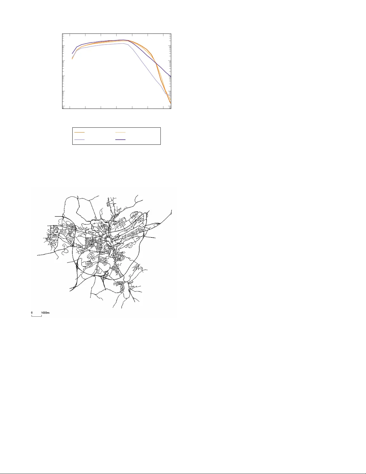
1 A Micro-Simulation Study of the Generalized Proportional Allocation T raf fic Signal Control Gustav Nilsson and Giacomo Como Abstract —In this paper , we study the pr oblem of determining phase activations for signalized junctions by utilizing feedback, more specifically , by measure the queue-lengths on the incoming lanes to each junction. The controller we ar e in vestigating is the Generalized Proportional Allocation (GP A) controller , which has previously been shown to have desired stability and throughput properties in a continuous av eraged dynamical model for queueing networks. In this paper , we provide and implement two discretized versions of the GP A controller in the SUMO micro simulator . W e also compare the GP A controllers with the MaxPressur e controller , a controller that requires more information than the GP A, in an artificial Manhattan-like grid. T o sho w that the GP A controller is easy to implement in a r eal scenario, we also implement it in a previously published realistic traffic scenario for the city of Luxembourg and compare its performance with the static controller pr ovided with the scenario. The simulations show that the GP A performs better than a static controller for the Luxembourg scenario, and better than the MaxPressur e pressur e contr oller in the Manhattan-grid when the demands are low . Index terms: Decentralized T raffic Signal Control, Micro- scopic T raffic Simulation I . I N T RO D U C T I O N While the first traf fic signals were controlled completely in open loop, various approaches hav e been taken to adjust the green light allocation based on the current traffic situation. T o mention a fe w , SCOO T [1], UT OPIA [2] and SCA TS [3]. Also, learning based approaches ha ve been taken, e.g., [4]. Howe ver , these approaches lack of formal stability , opti- mality , and robustness guarantees. In [5], [6], a decentralized feedback controller for traf fic control was proposed, refereed to as Generalized Proportional Allocation (GP A) controller , which has both stability and maximal throughput guarantees. In those papers, an av erage control action for traffic signals in continuous time is given. Since the controller has se veral de- sired properties, it is motiv ated to in vestigate if this controller performs well in a micro-simulator with more realistic traf fic dynamics. First of all, under the assumptions that the controller can measure the whole queue lengths at each junction, the av eraged controller is throughput optimal from a theoretical perspectiv e. With this, we mean that when the traffic dynamics is modeled as a simple system of point queues there exists no G. Nilsson is with the Department of Automatic Control, Lund University , Sweden. gustav.nilsson@control.lth.se G. Como is with the Department of Mathematical Sciences, Politecnico di T orino, Italy , and the Department of Automatic Control, Lund University , Sweden. giacomo.como@polito.it The authors are members of the excellence centers LCCC and ELLIT . This reasearch was carried on within the framework of the MIUR-funded Pr ogetto di Eccellenza of the Dipartimento di Scienze Matematiche G.L. Lagr ange , CUP: E11G18000350001, and was partly supported by the Compagnia di San P aolo and the Swedish Research Council (VR). controller that can handle larger constant exogenous inflows to a network than this controller . This property of throughput- optimality also means that there are formal guarantees that the controller will not create gridlock situations in the network. As ex emplified in [7], feedback controllers that perform well for a single isolated junction may cause gridlock situations in a network setting. At the same time, this controller requires very little in- formation about the network topology and the traffic flo w propagation. All information the controller needs to determine the phase activ ation in a junction is the queue lengths on the incoming lanes to a junction and the static set of phases. Those requirements on information make the controller fully distributed, i.e., to compute the control action in one junc- tion, no information is required about the state in the other junctions. The proposed traffic signal controller also has the property that it adjusts the cycle lengths depending on the demand. The fact that during higher demands, the cycle lengths should be longer to waste less service time due to phase shifts, has been suggested previously for open loop traf fic signal control, see e..g [8]. Another feedback control strategy for traffic signal control is the MaxPressure controller [9], [7]. The MaxPressure con- troller utilizes the same idea as the BackPressure controller, proposed for communication networks in [10]. While the BackPressure controller controls both the routing (to which packets the should proceed after receiv ed service) and the scheduling (which subset of queues that should be severed), the MaxPressure controller only controls the latter , i.e., the phase activ ation b ut not the routing. More recently , due to the rapid dev elopment of autonomous v ehicles, it has been proposed in [11] to utilize the routing control from the BackPressure controller in traffic networks as well. The Max- Pressure controller is also throughput optimal, but it requires information about the tuning ratios at each junction, i.e., how the vehicles (in av erage) propagate from one junction to the neighboring junctions. Although various techniques for esti- mating those turning ratios have been made, for example [12], with more and more drivers or autonomous vehicles doing their path planning through some routing service, it is likely to belie ve that the turning ratios can change in an unpredictable way when a disturbance occurs in the traf fic network. If the traf fic signal controller has information about the turning ratios, other control strategies are possible as well, for instance, MPC-like as proposed in [13], [14], [15] and rob ust control as proposed in [16]. In [17] we presented the first discretization and v alidation results of the GP A in a microscopic traffic simulator . Although, 2 the results were promising, the validations were only per- formed on an artificial network and only compared with a fixed timed traf fic signal controller . Moreover , the GP A was only discretized in a w ay such that the full cycle is activ ated. In this paper , we extend the results in [17] by showing another discretization that does not ha ve to utilize the full cycle and we also perform new validations. The new validations both compare the GP A to the MaxPressure controller on an artificial network (the reason for chosen a artificial network will be explained later), but also v alidate the GP A controller in a realistic scenario, namely for the Luxembour g city during a whole day . The outline of the paper is as follo ws: In Section II we present the model we are using for traf fic signals, together with a problem formulation of the traffic signal control problem. In Section III we present two different discretization of the GP A that we are using in this study , but also giv e a brief description of the MaxPressure controller . In Section IV we compare the GP A controller with the MaxPressure controller on an artificial Manhattan-like grid, and in Section V we in vestigate how the GP A controller performs in a realistic traffic scenario. The paper is concluded with some ideas about further research. A. Notation W e let R + denote the non-negati ve reals. For a finite sets A , B , we let R A + denote non-negati ve vectors indexed by the elements in A , and R A×B + the matrices indexed by elements A and B . I I . M O D E L A N D P RO B L E M F O R M U L A T I O N In this section, we describe the model for traf fic signals to be used throughout the paper together with the associated control problem. W e consider an arterial traffic network with signalized junctions. Let J denote the set of signalized junctions. For a junction j ∈ J , we let L ( j ) be the set of incoming lanes, on which the vehicles can queue up. The set of all signalized lanes in the whole network will be denoted by L = ∪ j ∈J L ( j ) . For a lane l ∈ L ( j ) , the queue-length at time t –measured in the number of vehicles– is denoted by x l ( t ) . Each junction has a predefined set of phases P ( j ) of size n p j . For simplicity , we assume that phases p i ∈ P ( j ) are index ed by i = 1 , . . . , n p j . A phase p ∈ P ( j ) is a subset of incoming lanes to the junction j that can receiv e green light simultaneously . Throughout the paper , we will assume that for each lane l ∈ L , there exists only one junction j ∈ J and at least one phase p ∈ P ( j ) such that l ∈ p . The phases are usually constructed such that the vehicles paths in a junction do not cross each other . This to av oid collisions. Examples of this will be sho wn later in this paper . After a phase has been activ ated, it is common to signalize to the dri vers that the traffic signal is turning red and gi ve time for vehicles that are in the middle of the junction to leav e it before the next phase are activ ated. Such time is usually referred to as clearance time. Throughout the paper we shall refer to those phases only containing red and yello w traf fic light as clear ance phases (in contrast to phases, that models when lanes receiv es l 1 l 2 l 3 l 4 l 1 l 2 l 3 l 4 Fig. 1. The phases for the junction in Example 1. This junction has four incoming lanes and two phases, p 1 = { l 1 , l 3 } and p 2 = { l 2 , l 4 } . Hence there is no specific lane left-turning left. t 0 25 30 55 60 c ( t ) p 1 p 0 1 p 2 p 0 2 Fig. 2. Example of a signal program for the junction in Example 1. In this example the signal program is T = { ( p 1 , 25) , ( p 0 1 , 30) , ( p 2 , 55) , ( p 0 2 , 60) } . green traffic light). W e will assume that each phase activ ation is followed by a clearance phase activ ation. While we will let the phase activ ation time vary , we will mak e the quite natural assumption that the clearance phases has to be activ ated for a fixed time. For a gi ven junction j ∈ J , the set of phases can be described through a phase matrix P ( j ) , where P il =  1 if lane l belongs to the i -th phase 0 if otherwise . While the phase matrix does not contain the clearance phases, to each phase p ∈ P ( j ) we will associate a clearance phase, denoted p 0 . W e denote the set of real phases and their corresponding clearance phases ¯ P ( j ) . The controller’ s task in a signalized junction is to define a signal pr ogram , T ( j ) = { ( p, t end ) ∈ ¯ P ( j ) × R + } , where the phase p is acti vated until t end . When t = t end , the phase p 0 , where ( p 0 , t end ) ∈ T ( j ) , with smallest t end > t is activ ated. Formally , we can define the function c ( j ) ( t ) that gi ves the phase that is activ ated at time t as follo ws c ( j ) ( t ) = { p : ( p, t end ) ∈ T ( j ) | t end > t and t end ≤ t 0 end for all ( p 0 , t 0 end ) ∈ T ( j ) } . What c ( j ) ( t ) is doing is to find the phase with the smallest end-time greater than the current time. Example 1: Consider the junction in Fig. 1 with the incoming lanes numbered as in the figure. In this case the driv ers turning left have to solve the collision av oidance by themselves. The phase matrix is P =  1 0 1 0 0 1 0 1  . An example of signal program is shown in Fig. 2. Here the program is T = { ( p 1 , 25) , ( p 0 1 , 30) , ( p 2 , 55) , ( p 0 2 , 60) } . which 3 means that both the phases are activ ated for 25 seconds each, and the clearance phases are acti vated for 5 seconds each. Moreov er, we let T ( j ) = max { t end | ( p, t end ) ∈ P ( j ) } denote the time when the signal program for junction j ends, and hence a new signal timing program has to be determined. I I I . F E E D BA C K C O N T RO L L E R S In this section, we present three dif ferent traffic signal controllers that all determine the signal program. The first two are discretization of the GP A controller, where the first one makes sure that all the clearance phase are activ ated during one cycle, and the second one only acti vates the clearance phases if their corresponding phase has been acti vated. The third controller is the MaxPressure controller . All the three controllers are feedback-based, i.e., when one signal program has reached its end, the current queue lengths are used to determine the upcoming signal program. Moreov er, the GP A controllers are fully distributed, in the sense that to determine the signal program in one junction, the controller only needs information about the queue-lengths on the incoming lanes for that junction. The MaxPressure controller is also distrib uted in the sense that it does not requires netw ork wide information, but it requires queue length information from the neighboring junctions as well. For all of the controller presented in this section, we assume for simplicity of the presentation that after a phase has been activ ated, a clearance phase has to be activ ated for a fixed amount of time T w > 0 , that is independent of which phase that has just been acti vated. A. GP A with Full Clearance Cycles For this controller, we assume that all the clearance phases hav e to be activ ated for each cycle. When t = T ( j ) , a new signal program is computed by solving the following con ve x optimization problem: maximize ν ∈ R n p j + w ∈ R + X l ∈L ( j ) x l ( t ) log  ( P T ν ) l  + κ log ( w ) , subject to X 1 ≤ i ≤ n p j ν i + w = 1 , w ≥ ¯ w . (1) In the optimization problem abov e, κ > 0 and ¯ w ≥ 0 are tuning parameters for the controller , and their interpretation will be discussed later . The vector ν in the solution of the optimization problem abov e, determines the fraction of the c ycle time that each phase should be acti vated, where each element in ν contains this fraction. The variable w tells how large fraction of the c ycle time that should be allocated to the clearance phases. Observe that as long as the queue lengths are finite w will be strictly greater than zero. Since we assume that each clearance phase has to be activ ated for a fix ed amount of time, T w > 0 , the total cycle length T cyc for the upcoming cycle can be computed by T cyc = n p j T w w . W ith the knowledge of the full-cycle length, the signal pro- gram for the upcoming cycle can be computed according to Algorithm 1. Although the optimization problem can be solved in real- time using con vex solvers, the optimization problem can also be solved analytically in the spacial cases. One such case is when the phases are orthogonal, i.e., every incoming lane only belongs to one phase. If the phases are orthogonal, then P T 1 = 1 . In the case of orthogonal phases and ¯ w = 0 , the solution to the optimization problem in (1) is gi ven by ν i ( x ( t )) = P l ∈L ( j ) P il x l ( t ) κ + P l ∈L ( j ) x l ( t ) , i = 1 , . . . , n p j , w ( x ( t )) = κ κ + P l ∈L ( j ) x l ( t ) . (2) From the e xpression of w abov e, a direct expression for the total c ycle length can be obtained T cyc = T w n p j + T w n p j κ X l ∈L ( j ) x l ( t ) . From the expressions abo ve we can observ e a few things. First, we see that the fraction of the cycle that each phase is activ ated is proportional to the queue lengths in that phase, and this explains why we done this control strategy generalized proportional allocation. Moreov er , we get an interpretation of the tuning parameter κ , it tells how the cycle length T cyc should scale with the current queue lengths. If κ is small, ev en small queue lengths will cause longer cycles, while if κ is large the cycles will be short even for large queues. Hence, a too small κ may giv e too long cycles, which can result in that lanes get more green-light than needed and the controller ends up giving green light to empty lanes, while vehicles in other lanes are waiting for service. On the other hand, a too large κ may make the cycle lengths so short, so that the fraction of the cycle that each phase gets activ ated is too short for the drivers to react on. Remark 1: In [6] we showed that the a veraged continuous time GP A controller can stabilize, and hence keep the queue- lengths bounded, the network. Moreover , this averaged version is throughput-optimal, which means that no controller can handle more exogenous inflo w to network than this controller . Howe ver , when the controller is discretized, the following example sho ws that an upper bound on the c ycle length, i.e., ¯ w > 0 is required to guarantee stability ev en for an isolated junction. Example 2: Consider a junction with two incoming lanes with unit flo w capacity , both having their o wn phase, and let the exogenous inflows λ 1 = λ 2 = λ , T w = 1 , ¯ w = 0 , x 1 (0) = 4 Algorithm 1: GP A with Full Clearance Cycles Data: Current time t , local queue lengths x ( j ) ( t ) , phase matrix P ( j ) , clearance time T w , tuning parameters κ, ¯ w Result: Signal program T ( j ) T ( j ) ← ∅ n p j ← Number of rows in P ( j ) ( ν, w ) ← Solution to (1) giv en x ( j ) ( t ) , P ( j ) , κ, ¯ w T cyc ← n p · T w /w t end ← t for i ← 1 to n p j do t end ← t end + ν i · T cyc T ( j ) ← T ( j ) + ( p i , t end )  Add phase p i t end ← t end + T w T ( j ) ← T ( j ) + ( p 0 i , t end )  Add clearance phase p 0 i end A > 0 , and x 2 (0) = 0 . The control signals and the cycle time for the first iteration is then giv en by u 1 ( x (0)) = A A + κ , u 2 ( x (0)) = 0 , T ( x (0)) = A + κ κ . Observe that the cycle time T ( x (0)) is strictly increasing with A . After one full service cycle, i.e., at t 1 = T ( x (0)) the queue lengths are x 1 ( t 1 ) = A + T ( x (0))  λ − A A + κ  = f ( A ) z }| { A + λ A + κ κ − A κ , x 2 ( t 1 ) = T ( x (0)) λ = λ  A + κ κ  . If x 1 ( t 1 ) = 0 , then due to symmetry , the analysis of the system can be repeated in the same w ay with a new initial condition. T o make sure that one queue alw ays get empty during the service cycles, it must hold that f ( A ) ≤ 0 . Moreover , to make sure that the other queue grows, it must also hold that x 2 ( t 1 ) > A which can be equi valently e xpressed as Aκ + λ ( A + κ ) − A ≤ 0 , Aκ − λ ( A + κ ) < 0 . The choice of λ = κ = 0 . 1 and A = 1 is one set of parameters satisfying the constraints above, and will hence make the queue lengths and cycle times grow unboundedly . How queue lengths and cycle times ev olve in this case is shown in Fig. 3. Imposing an upper bound on the cycle length, and hence a lower bound on w will then shrink the throughput region. An upper bound of the c ycle length may occurs naturally , due to the fact that the sensors cover a limited area and hence the measurements will saturate. Howe ver , we will later observe in the simulations that ¯ w > 0 may improv e the performance of the controller when it is simulated in a realistic scenario, even when saturation of the queue length measurements is possible. 0 100 200 300 400 500 0 2 4 T ime t Queue length x 1 x 2 0 5 10 15 20 25 0 2 4 6 8 Cycle k Cycle time T ( x ( t k )) Fig. 3. How the traffic volumes ev olve in time together with the cycle times for the system in Example 2. W e can observe that the cycle length increases for each cycle. B. GP A with Shorted Cycles One possible drawback of the controller in Section III-A is that it has to activ ate all the clearance phases in one cycle. This property implies that if the junction is empty when the signal program is computed, it will take n p j T w seconds until a new signal program is computed. Moti vated by this, we also present a version of the GP A where only the clearance phases get activ ated if their corresponding phases have been acti vated. If we let n 0 p j denote the number of phases that will be activ ated during the upcoming cycle, the total cycle time is gi ven by T cyc = n 0 p j T w w . How to compute the signal program in this case, is shown in Algorithm 2. C. MaxPr essur e As mentioned in the introduction, the MaxPressure con- troller is another throughput optimal feedback controller for traffic signals. The controller computes the difference between the queue lengths and their do wnstream queue lengths in each phase, to determine each phase’ s pressure. It then activ ates the phase with the most pressure for a fixed time interval. T o compute the pressure, the controller needs information about where the outflow from ev ery queue will proceed. T o model this, we introduce the routing matrix R ∈ R E ×E + , whose elements R ij tells the fraction of vehicles that will proceed from lane i in the current junction to lane j in a downstream junction. W ith the kno wledge of the routing matrix and under the assumption that the flo w rates are the same for all phases, the 5 Algorithm 2: GP A with Shorted Cycles Data: Current time t , local queue lengths x ( j ) ( t ) , phase matrix P ( j ) , clearance time T w , tuning parameters κ, ¯ w Result: Signal program T ( j ) T ( j ) ← ∅ n p j ← Number of rows in P ( j ) ( ν, w ) ← Solution to (1) giv en x ( j ) ( t ) , P ( j ) , κ, ¯ w  Compute the number of phases to be acti vated n 0 p j ← 0 for i ← 1 to n p j do if ν i > 0 then n 0 p j ← n 0 p j + 1 end end if n 0 p j > 0 then  If vehicles are present on some phases, activ ate those T cyc ← n 0 p j · T w /w t end ← t for i ← 1 to n p do if ν i > 0 then t end ← t end + ν i · T cyc  Add phase p i T ( j ) ← T ( j ) + ( p i , t end ) t end ← t end + T w  Add clearance phase p 0 i T ( j ) ← T ( j ) + ( p 0 i , t end ) end end else  If no vehicles are present, hold a clearance phase for one time unit T ( j ) ← ( p 0 1 , t + 1) end pressure, w i , for each phase p i ∈ P j can then be computed as w i = X l ∈ p i  x l ( t ) − X k R lk x k ( t )  . The phase that should be activ ated is then any phase in the set argmax i w i . Apart from the routing matrix, the MaxPressure controller has one tuning parameter , the phase duration d > 0 . That pa- rameter tells how long a phase should be activ ated, and hence how long it should take until the pressures are resampled, and a ne w phase acti vation decision is made. How to compute the signal program with the MaxPressure controller is shown in Algorithm 3. I V . C O M PA R I S O N B E T W E E N G P A A N D M A X P R E S S U R E A. Simulation setting T o compare the proposed controller and the MaxPres- sure controller , we simulate both controllers on an artificial Algorithm 3: MaxPressure Data: Current time t , local queue lengths x ( t ) , phase matrix P ( j ) , routing matrix R , phase duration d Result: Signal program T ( j ) T ( j ) ← ∅ n p j ← Number of rows in P ( j ) for i ← 1 to n p j do for l ∈ L ( j ) do if l ∈ p ( j ) i then w i ← w i + x l ( t ) − P k R lk x k ( t ) end end end i ← argmax i w i  Add phase p i T ( j ) ← T ( j ) + ( p i , t + d )  Add clearance phase p 0 i T ( j ) ← T ( j ) + ( p 0 i , t + d + T w ) 1 2 3 4 5 6 7 8 9 10 A B C D E F G H I J Fig. 4. The Manhattan-like network used in the comparison between GP A and MaxPressure. Manhattan-like grid with artificial demand. The simulator we are using is open source micro simulator SUMO [18], which is a simulator that simulates ev ery single vehicle’ s behavior in the traffic network. A schematic drawing of the network is shown in Fig. 4. In a setting like this, we can elaborate with the tuning ratios, and provide the MaxPressure controller both correct and incorrect turning ratios. This allows us to in vestigate the robustness properties of both the controllers. The Manhattan grid in Fig. 4 has ten bidirectional north to south streets (indexed A to J) and ten bidirectional east to west streets (indexed 1 to 10). All streets with an odd number or indexed by letter A, C, E, G or I consist of one lane in each direction, while the others consist of two lanes in each direction. The speed limit on each lane is 50 km/h. The distance between each junction is three hundred meters. Fifty meters before each junction, every street has an additional lane, reserved for vehicles that want to turn left. Due to the v arying number of lanes, four different junction topologies exist, all shown in Fig. 5, together with the set of possible phases. Each junction is equipped with sensors on the incoming lanes that 6 2 by 2 junction 2 by 3 junction 3 by 2 junction 3 by 3 junction Fig. 5. The four different types of junctions present in the Manhattan grid, together with theirs phases. can measure the number of vehicles queuing up to fifty meters from the junction. The sensors measure the queue lengths by the number of stopped vehicles. Since the scenario is artificial, we can generate demand with prescribed turning ratios and hence let the MaxPressure controller to run in an ideal setting. For the demand generation, we assume that at each junction a vehicle will with probability 0 . 2 will turn left, with probability 0 . 6 go straight and with probability 0 . 2 turn right. W e do assume that all vehicles depart from lanes connected to the boundary of the network, and all vehicles will also end their trips when they have reached the boundary of the network. In other words, no vehicles will depart or arriv e inside the grid. W e will study the controllers’ performance for three dif ferent demands, where the demand determined by the probability that a vehicle will depart from each boundary lane each second. W e denote this probability δ , where the probabilities for the three different demands are δ = 0 . 05 , δ = 0 . 1 and δ = 0 . 15 . W e generate vehicles for 3600 seconds and then simulate until all vehicles hav e left the netw ork. W e also compare the results for the GP A controller and the MaxPressure controller with a standard fixed time (FT) controller and a proportional fair (PF) controller , i.e., the GP A controller with full clearance c ycles, but with κ = 0 and a prescribed fixed cycle length. For the fixed time controller , the phases which contain a straight movement are activ ated for 30 seconds and phases only containing left or right turn mov ements are acti v ated for 15 seconds. The clearance time for each phase is still set to 5 seconds. This means that the cycle lengths for each of the four types of junctions will be 110 seconds. This is also the fixed cycle time we are using for the proportional fairness controller . T ABLE I G P A W I T H S H ORT E D C Y C LE S - M A N HATTA N S C EN A RI O κ δ T otal Tra vel Time [h] 1 0 . 05 1398 5 0 . 05 715 10 0 . 05 699 15 0 . 05 696 20 0 . 05 690 1 0 . 10 7636 5 0 . 10 1898 10 0 . 10 1992 15 0 . 10 2263 20 0 . 10 2495 1 0 . 15 + ∞ 5 0 . 15 5134 10 0 . 15 4498 15 0 . 15 5140 20 0 . 15 6050 0 1 , 000 2 , 000 3 , 000 4 , 000 5 , 000 6 , 000 10 0 10 1 10 2 10 3 10 4 T ime [s] T otal Queue Length [m] GP A κ = 10 δ = 0 . 05 GP A κ = 10 δ = 0 . 10 GP A κ = 10 δ = 0 . 15 GP A κ = 5 δ = 0 . 05 GP A κ = 5 δ = 0 . 10 GP A κ = 5 δ = 0 . 15 Fig. 6. How the queue length varies with time when the GP A with shorted cycles are used in Manhattan grid. The GP A is tested with two different values of κ = 5 , 10 for the three demand scenarios δ = 0 . 05 , 0 . 10 , 0 . 15 . T o improve the readability of the results, the queue-lengths are averaged over 300 seconds intervals. B. GP A Results Since the phases in this scenario are all orthogonal, the expressions in (2) can be used to solve the optimization problem in (1). The tuning parameter ¯ w is set to ¯ w = 0 for all simulations. In T able I we show ho w the total travel time varies for the GP A controller with shorted cycles for different values of κ . F or the demand δ = 0 . 15 and κ = 1 a gridlock situation occurs, probably due to the fact that vehicles back- spills into upstream junctions. W e can see that a κ = 10 seems to be the best choice for δ = 1 and δ = 0 . 15 , while a higher κ slightly improves the total trav el time for the lowest demand in vestigated. Letting κ = 10 has been shown to be reasonable for other demand scenarios in the same network setting, as observed in [17]. How the total queue lengths varies with time for κ = 5 and κ = 10 is sho wn in Fig. 6. 7 T ABLE II M A X P R E S SU R E - M A N H A T T A N S C EN AR I O d δ TTT correct TR [h] TTT incorrect TR [h] 10 0 . 05 858 856 20 0 . 05 1 079 1 102 30 0 . 05 1 172 1 193 10 0 . 10 1 865 1 864 20 0 . 10 2 254 2 312 30 0 . 10 2 690 2 718 10 0 . 15 3 511 3 488 20 0 . 15 3 992 4 102 30 0 . 15 5 579 5 590 C. MaxPr essur e Results The MaxPressure controller decides its control action not only based on queue-lengths on the incoming lanes, but also on the downstream lanes. It is not always clear in which downstream lane a vehicle will end up in after leaving the junction. If a vehicle can choose between several lanes that are all valid for its path, the vehicle’ s lane choice will be determined during the simulation, and depend upon how many other vehicles that are occupying the possible lanes. Because of this, we assume that if a vehicle can choose between sev eral lanes, it will try to join the shortest one. T o exemplify how the turning ratios are estimated in those situations, assume that Moreov er, assume that the overall probability that a vehicle is turning right is 0 . 2 , and going straight is 0 . 6 . If a vehicle going straight can choose between lane l 1 , l 2 , but l 2 is also used by vehicles turning right, the probability that the vehicle going straight will queue up in lane l 1 is assumed to be 0 . 4 and that the probability that the vehicle will queue up in lane l 2 is estimated to be 0 . 2 . T o also inv estigate the MaxPressure controller’ s rob ustness with respect to the routing information, we perform simu- lations both when the controller has the correct information about the turning probabilities, i.e., that a vehicle will turn right with probability 0 . 2 , continue straight with probability 0 . 6 and turn left with probability 0 . 2 . For the simulations when the MaxPressure has the wrong turning information, the controller instead has the information that with probability 0 . 6 the vehicle will turn right, with probability 0 . 3 the vehicle will proceed straight and with probability 0 . 1 the vehicle will turn left. In the simulations, we consider three different phase durations, d = 10 seconds, d = 20 seconds and d = 30 seconds. How the total queue lengths vary ov er time for the different demands is shown in Fig. 7, Fig. 8, and Fig. 9. The total trav el time, both when the MaxPressure controller is operating with the right, and the wrong turning ratios are shown in T able II. From these results, we can conclude that a shorter phase duration, i.e., d = 10 , is the most efficient for all demands. This probably has to do with a longer phase duration the activ ation time is becoming larger than the time it takes to empty the measurable part of the queue. Another interesting observation is that if the MaxPressure controller has wrong information about the turning ratios, its performance does not decrease significantly . 0 1 , 000 2 , 000 3 , 000 4 , 000 5 , 000 0 2 000 4 000 T ime [s] T otal Queue Length [m] MP d = 10 MP d = 20 MP d = 30 Fig. 7. The total queue length ov er time in the Manhattan grid with the MaxPressure (MP) controller with right turning ratios (solid) and wrong turning ratios (dashed). The demand is δ = 0 . 05 . T o improv e the readability of the results, the queue-lengths are averaged over 300 seconds intervals. 0 1 , 000 2 , 000 3 , 000 4 , 000 5 , 000 0 5 000 10 000 T ime [s] T otal Queue Length [m] MP d = 10 MP d = 20 MP d = 30 Fig. 8. The total queue length ov er time in the Manhattan grid with the MaxPressure (MP) controller with right turning ratios (solid) and wrong turning ratios (dashed). The demand is δ = 0 . 10 . T o improv e the readability of the results, the queue-lengths are averaged over 300 seconds intervals. D. Summery of the Comparison T o better observe the difference between the GP A and MaxPressure, we have plotted the total queue length with the GP A controller with κ = 5 and κ = 10 , and the best MaxPressure configuration with d = 10 . The results are sho wn in Fig. 10, Fig. 11 and Fig. 12. In the figures we hav e also included for reference the total queue lengths for the fixed time controller and the proportional fair controller . The total trav el tra vel times for those controllers are giv en in T able III. When the demand is δ = 0 . 15 , a gridlock situation occurs with the proportional fair controller , just as happened with the GP A controller with κ = 1 . From the simulations, we can conclude that, for this scenario, during high demands, the MaxPressure 8 0 1 , 000 2 , 000 3 , 000 4 , 000 5 , 000 6 , 000 0 10 000 20 000 T ime [s] T otal Queue Length [m] MP d = 10 MP d = 20 MP d = 30 Fig. 9. The total queue length ov er time in the Manhattan grid with the MaxPressure (MP) controller with right turning ratios (solid) and wrong turning ratios (dashed). The demand is δ = 0 . 15 . T o improv e the readability of the results, the queue-lengths are averaged over 300 seconds intervals. T ABLE III F I XE D T I M E A N D P RO P O RT IO N AL F A IR C O NT R OL - M A N HAT T A N S C EN A RI O Controller δ T otal Tra vel Time [h] FT 0 . 05 1201 FT 0 . 10 2555 FT 0 . 15 4642 PF 0 . 05 1694 PF 0 . 10 4165 PF 0 . 15 + ∞ controller performs better than the GP A controller , while during low demands the GP A performs better . One explanation for this could be that during low demands, adopting the cycle length is critical, while during high demands when almost all the sensors are covered, it is more important to keep the queue balanced between the current and downstream lanes. The proportional fair controller that does not adopt its cycle length, performs always the w orst, and in most of the cases a fixed time controller performs second worst. It is just for the demand δ = 0 . 15 , and during the draining phase that the fixed time controller performs better than the GP A controller . V . L U S T S C E N A R I O T o test the proposed controller in a realistic scenario, we make use of the Luxembourg SUMO T raffic (LuST) scenario presented in [19] 1 . The scenario models the city center of Luxembour g during a full day , and the authors of [19] hav e made se veral adjustments from some given population data when creating the scenario, to make it as realistic as possible. The LuST network is shown in Fig. 13. T o each of the 199 signalized junctions, we hav e added a lane area detector to each incoming lane. The length of the detectors are 100 meters, or as long as the lane is if it is shorter than 100 meters. Those 1 The scenario files are obtained from https://github .com/lcodeca/ LuSTScenario/tree/v2.0 0 1 , 000 2 , 000 3 , 000 4 , 000 5 , 000 10 0 10 1 10 2 10 3 10 4 T ime [s] T otal Queue Length [m] GP A κ = 5 GP A κ = 10 MP d = 10 Fixed Time PF Fig. 10. A comparison between different control strategies for the Manhattan grid with the demand δ = 0 . 05 .o improve the readability of the results, the queue-lengths are averaged over 300 seconds intervals. 0 1 , 000 2 , 000 3 , 000 4 , 000 5 , 000 10 0 10 1 10 2 10 3 10 4 T ime [s] T otal Queue Length [m] GP A κ = 5 GP A κ = 10 MP d = 10 Fixed Time PF Fig. 11. A comparison between different control strategies for the Manhattan grid with the demand δ = 0 . 10 . T o improve the readability of the results, the queue-lengths are averaged over 300 seconds intervals. sensors are added to giv e the controller real-time information about the queue-lengths at each junction. As input to the system, we are using the Dynamic User Assignment demand data. For this data-set, the drivers try to take their shortest path (with respect to time) between their current position and destination. It is assumed that 70 percent of the vehicles can recompute their shortest path while driving, and will do so every fifth minute. This rerouting possibility is introduced in order to model the fact that more and more driv ers are using online navigation with real-time traf fic state information, and will hence get updates about what the optimal route choice is. In the LuST scenario, the phases are constructed in a bit more complex way and are not always orthogonal. For non- orthogonal phases, it is not always the case that all lanes 9 0 1 , 000 2 , 000 3 , 000 4 , 000 5 , 000 6 , 000 10 0 10 1 10 2 10 3 10 4 T ime [s] T otal Queue Length [m] GP A κ = 5 GP A κ = 10 MP d = 10 Fixed Time Fig. 12. A comparison between different control strategies for the Manhattan grid with the demand δ = 0 . 15 . Since the proportional fair controller (PF) creates a gridlock, it is not included in the comparison. T o improve the readability of the results, the queue-lengths are averaged over 300 seconds intervals. Fig. 13. The traffic network of Luxembourg city receiv e yello w light when a clearance phase is acti vated. If the lane recei ves a green light in the next phase as well, it will receiv e green light during the clearance phase too. This property makes it more dif ficult to shorten the cycle, and for that reason, we choose to implement the controller which acti v ates all the clearance phases in the c ycle, i.e., the controller gi ven in Section III-A. As mentioned, the phases in the LuST scenario are not or - thogonal in each junction. Hence we hav e to solve the con vex optimization problem in (1) to compute the phase activ ation. The computation is done by using the solver CVXPY 2 in Python. Although the controller can be implemented in a distributed manner , the simulations are in this paper performed 2 https://cvxpy .org on a single computer . Despite the size of the network, and that the communication via TraCI between the controller written in Python and SUMO slo ws do wn the simulations significantly , the simulations are still running about 2 . 5 times faster than real-time. This shows that there is no problem with running this controller in a real-time setting. Since the demand is high during the peak-hours in the scenario, gridlock situations occur . Those kinds of situations is unavoidable since there will be conflicts in the car following model. T o make the simulation continue to run, SUMO has a teleporting option that is utilized in the original LuST scenario. The original LuST scenario is configured such that if that a vehicle has been looked for more than 10 minutes, it will teleport along its route until there is free space. It is therefore important when we ev aluate the control strategies that we keep track of the number of teleports, to make sure that the control strategy will not create a significantly larger amount of gridlocks, compared to the original fixed time controller . In T able IV the number of teleports are reported for each controller . It is also reported ho w many of those teleports that are caused directly due to traf fic jam, b ut one should have in mind that e.g., a gridlock caused by that two vehicles want to swap lanes, is often a consequence of a congestion. The total trav el time and the number of teleports for different choices of tuning parameters are sho wn in T able IV. For the fixed time controller , we k eep the standard fixed time plan provided with the LuST scenario. How the queue lengths vary with time for different ¯ w is sho wn in Fig. 14 for κ = 5 and in Fig. 15 for κ = 10 . From the results, we can see that any controller with κ = 10 and ¯ w within the range of inv estigation will improv e the traffic situation. Ho wev er , the controller that yields the ov erall shortest total trav el time is the one with κ = 5 and ¯ w = 0 . 40 . This result suggests that tuning the GP A only with respect to κ , and keep ¯ w = 0 , may not lead to the best performance with respect to total tra vel time, although it gives higher theoretical throughput. V I . C O N C L U S I O N S In this paper, we ha ve discussed implementational aspects of the Generalized Proportional Allocation controller . The controller’ s performance was compared to the MaxPressure controller both on an artificial Manhattan-like grid and for a real scenario. In comparison with MaxPressure, it was shown that the controller performs better than the MaxPressure controller when the demand is low , but the MaxPressure performs better during high demand. Those observ ations hold true e ven if the MaxPressure controller does not have correct information about the turning ratios in each junction. While the information about the turning ratios and the queue lengths at neighboring junctions are needed for the MaxPressure controller , the GP A controller does not require any such information. This makes the GP A controller easier to implement in a real scenario, where the downstream junction may not be signalized and equipped with sensors. W e sho wed that it is possible to both implement the GP A controller in a realistic scenario cov ering the city of Luxembourg and that 10 T ABLE IV C O MPA R IS O N O F T H E D I FFE R E N T C O N TR O L S T R A T E G IE S κ ¯ w T eleports (jam) T otal Trav el Time [h] GP A 10 0 76 (6) 49 791 GP A 10 0 . 05 65 (1) 49 708 GP A 10 0 . 10 37 (0) 49 519 GP A 10 0 . 15 57 (19) 49 408 GP A 10 0 . 20 50 (10) 49 380 GP A 10 0 . 25 35 (0) 49 265 GP A 10 0 . 30 30 (0) 48 930 GP A 10 0 . 35 25 (1) 48 922 GP A 10 0 . 40 51 (0) 48 932 GP A 10 0 . 45 49 (5) 49 076 GP A 10 0 . 50 42 (15) 49 383 GP A 5 0 668 (76) 57 249 GP A 5 0 . 05 234 (62) 54 870 GP A 5 0 . 10 68 (10) 52 038 GP A 5 0 . 15 47 (9) 50 696 GP A 5 0 . 20 50 (6) 49 904 GP A 5 0 . 25 41 (3) 49 454 GP A 5 0 . 30 23 (0) 48 964 GP A 5 0 . 35 30 (1) 48 643 GP A 5 0 . 40 35 (5) 48 445 GP A 5 0 . 45 39 (1) 48 503 GP A 5 0 . 50 42 (10) 48 772 Fixed time – – 122 (80) 54 103 0 : 00 4 : 00 8 : 00 12 : 00 16 : 00 20 : 00 24 : 00 10 2 10 3 10 4 T ime T otal Queue Length [m] GP A ¯ w = 0 GP A ¯ w = 0 . 1 GP A ¯ w = 0 . 2 GP A ¯ w = 0 . 3 GP A ¯ w = 0 . 4 Fixed Time Fig. 14. How the queue lengths varies with time when the traffic lights in the LuST scenario are controlled with the GP A controller and the standard fixed time controller . For the GP A controller the paramters κ = 5 and different values of ¯ w are tested. In order to improve the readability of the results, the queue-lengths are averaged over 300 seconds intervals. 0 : 00 4 : 00 8 : 00 12 : 00 16 : 00 20 : 00 24 : 00 10 2 10 3 10 4 T ime T otal Queue Length [m] GP A ¯ w = 0 GP A ¯ w = 0 . 1 GP A ¯ w = 0 . 2 GP A ¯ w = 0 . 3 GP A ¯ w = 0 . 4 Fixed Time Fig. 15. How the queue lengths varies with time when the traffic lights in the LuST scenario are controlled with the GP A controller and the standard fixed time controller . For the GP A controller the paramters κ = 10 and different values of ¯ w are tested. In order to improve the readability of the results, the queue-lengths are averaged over 300 seconds intervals. it improves the traffic situation compared to a standard fixed time controller . In all simulations, we hav e used the same tuning parameters for all junctions in the LuST scenario, while the fixed time controller is different for different junction settings. Hence the GP A controller’ s performance can be even more improved by tuning the parameters specifically for each junction. Ideally , this should be done with some auto-tuning solution, but it may also be worth to take static parameters into account, such as the sensor lengths. This is a topic for future research. R E F E R E N C E S [1] D. I. Robertson and R. D. Bretherton, “Optimizing networks of traffic signals in real time-the SCOO T method, ” IEEE T ransactions on vehic- ular technology , vol. 40, no. 1, pp. 11–15, 1991. [2] V . Mauro and C. Di T aranto, “Utopia, ” in Control, computers, commu- nications in transportation , pp. 245–252, Elsevier , 1990. [3] A. G. Sims and K. W . Dobinson, “The Sydney coordinated adaptiv e traffic (SCA T) system philosophy and benefits, ” IEEE T ransactions on vehicular technology , vol. 29, no. 2, pp. 130–137, 1980. [4] J. Jin and X. Ma, “ A decentralized traffic light control system based on adaptiv e learning, ” IF AC-P apersOnLine , vol. 50, no. 1, pp. 5301 – 5306, 2017. 20th IF A C W orld Congress. [5] G. Nilsson, P . Hosseini, G. Como, and K. Savla, “Entrop y-like Lyapunov functions for the stability analysis of adaptive traffic signal controls, ” in The 54th IEEE Conference on Decision and Contr ol , pp. 2193–2198, 2015. [6] G. Nilsson and G. Como, “On generalized proportional allocation policies for traffic signal control, ” IF AC-P apersOnLine , vol. 50, no. 1, pp. 9643–9648, 2017. [7] P . V araiya, “Max pressure control of a network of signalized intersec- tions, ” T ransportation Resear ch P art C: Emerging T echnologies , vol. 36, pp. 177–195, 2013. 11 [8] R. P . Roess, E. S. Prassas, and W . R. McShane, T raffic engineering . Prentice Hall, 2011. [9] P . V araiya, “The max-pressure controller for arbitrary networks of signalized intersections, ” in Advances in Dynamic Network Modeling in Complex T ransportation Systems , pp. 27–66, Springer, 2013. [10] L. T assiulas and A. Ephremides, “Stability properties of constrained queueing systems and scheduling policies for maximum throughput in multihop radio networks, ” IEEE T ransactions on Automatic Control , vol. 37, no. 12, pp. 1936–1948, 1992. [11] A. A. Zaidi, B. Kulcs ´ ar , and H. W ymeersch, “Back-pressure traffic signal control with fixed and adapti ve routing for urban vehicular networks, ” IEEE T ransactions on Intelligent T ransportation Systems , vol. 17, pp. 2134–2143, Aug 2016. [12] S. Coogan, C. Flores, and P . V araiya, “T raffic predictiv e control from low-rank structure, ” T ransportation Resear ch P art B: Methodological , vol. 97, pp. 1–22, 2017. [13] Z. Hao, R. Boel, and Z. Li, “Model based urban traffic control, part i: Local model and local model predictive controllers, ” T ransportation Resear ch P art C: Emerging T echnologies , vol. 97, pp. 61 – 81, 2018. [14] Z. Hao, R. Boel, and Z. Li, “Model based urban traffic control, part ii: Coordinated model predictive controllers, ” Tr ansportation Research P art C: Emerging T echnologies , vol. 97, pp. 23 – 44, 2018. [15] P . Grandinetti, C. Canudas-de Wit, and F . Garin, “Distributed optimal traffic lights design for large-scale urban networks, ” IEEE T ransactions on Contr ol Systems T echnology , 2018. [16] G. Bianchin and F . Pasqualetti, “ A network optimization framework for the analysis and control of traffic dynamics and intersection signaling, ” in 57th IEEE Conference on Decision and Control , pp. 1017–1022, Dec 2018. [17] G. Nilsson and G. Como, “Evaluation of decentralized feedback traffic light control with dynamic cycle length, ” IF AC-P apersOnLine , vol. 51, no. 9, pp. 464–469, 2018. [18] D. Krajzewicz, J. Erdmann, M. Behrisch, and L. Bieker , “Recent devel- opment and applications of SUMO - Simulation of Urban MObility , ” International Journal On Advances in Systems and Measurements , vol. 5, pp. 128–138, December 2012. [19] L. Codec ´ a, R. Frank, S. Faye, and T . Engel, “Luxembourg SUMO T raffic (LuST) Scenario: Traf fic Demand Evaluation, ” IEEE Intelligent T ransportation Systems Magazine , vol. 9, no. 2, pp. 52–63, 2017. Gustav Nilsson received his Master of Engineering Physics degree from Lund University in 2013. Since then, he has been a PhD student at the Department of Automatic Control, Lund University , working with Prof. Giacomo Como. During his PhD studies, he has done longer research visits to Institute of Pure and Applied Mathematics (IP AM), UCLA, CA, USA and Department of Mathematical Sciences, Politec- nico di T orino, T urin, Italy . Between October 2017 and March 2018, he did an internship at Mitsubishi Electric Research Laboratories in Cambridge, MA, USA. His primary research interest lies in modeling and control of dynamical flow networks with applications in transportation networks. Giacomo Como is an Associate Professor at the Department of Mathematical Sciences, Politecnico di T orino, Italy , and at the Automatic Control De- partment of Lund University , Sweden. He received the B.Sc., M.S., and Ph.D. degrees in Applied Math- ematics from Politecnico di T orino, in 2002, 2004, and 2008, respectively . He was a V isiting Assistant in Research at Y ale Uni versity in 2006-2007 and a Postdoctoral Associate at the Laboratory for Infor- mation and Decision Systems, Massachusetts Insti- tute of T echnology , from 2008 to 2011. He currently serves as Associate Editor of IEEE-TCNS and IEEE-TNSE and as chair of the IEEE-CSS T echnical Committee on Networks and Communications. He was the IPC chair of the IF AC W orkshop NecSys’15 and a semiplenary speaker at the International Symposium MTNS’16. He is recipient of the 2015 George S. Axelby Outstanding Paper award. His research interests are in dynamics, information, and control in network systems with applications to cyber-physical systems, infrastructure networks, and social and economic networks.