Estimating multi-year 24/7 origin-destination demand using high-granular multi-source traffic data

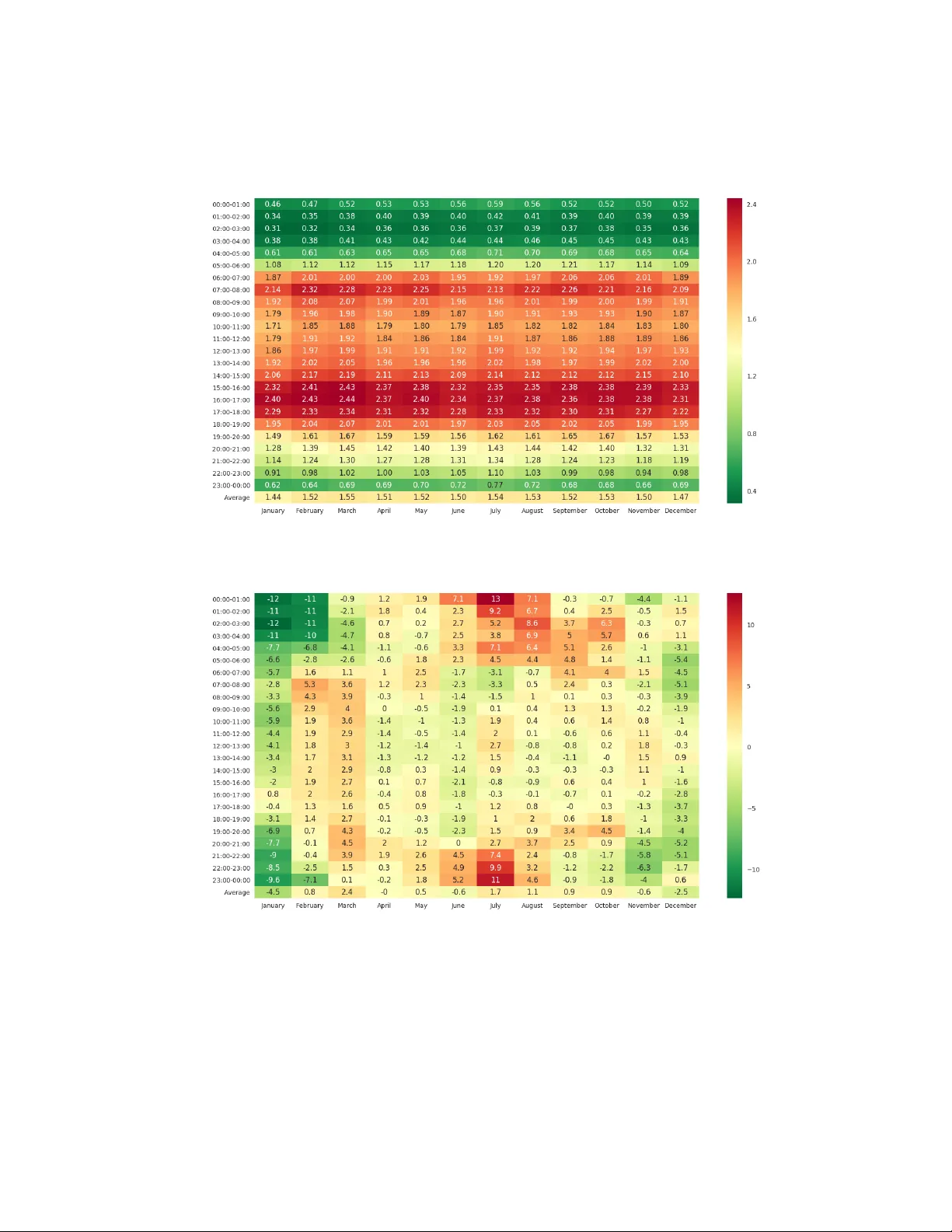
Estimating multi-year 24 / 7 origin-destination demand using high-granular multi-source traf fic data W ei Ma, Zhen (Sean) Qian Department of Ci vil and En vironmental Engineering Carnegie Mellon Uni versity , Pittsb urgh, P A 15213 { weima, seanqian } @cmu.edu December 20, 2024 Abstract Dynamic origin-destination (OD) demand is central to transportation system modeling and analysis. The dynamic OD demand estimation problem (DODE) has been studied for decades, most of which solve the DODE problem on a typical day or se veral typical hours. There is a lack of methods that estimate high-resolution dynamic OD demand for a sequence of many consecutiv e days over se veral years (referred to as 24/7 OD in this research). Having multi-year 24/7 OD demand would allow a better understanding of characteristics of dynamic OD demands and their ev olution/trends ov er the past few years, a critical input for modeling trans- portation system ev olution and reliability . This paper presents a data-driv en frame- work that estimates day-to-day dynamic OD using high-granular traf fic counts and speed data collected over many years. The proposed framework statistically clus- ters daily traffic data into typical traffic patterns using t-Distributed Stochastic Neighbor Embedding (t-SNE) and k-means methods. A GPU-based stochastic projected gradient descent method is proposed to ef ficiently solve the multi-year 24/7 DODE problem. It is demonstrated that the new method ef ficiently estimates the 5 -minute dynamic OD demand for e very single day from 2014 to 2016 on I-5 and SR-99 in the Sacramento region. The resultant multi-year 24/7 dynamic OD demand re veals the daily , weekly , monthly , seasonal and yearly change in travel demand in a region, implying intriguing demand characteristics o ver the years. 1 Intr oduction The increasing complexity and inter-connecti vity of mobility systems call for large- scale deployment of dynamic network models that encapsulate traffic flow ev olution for system-wide decision making. As an indispensable component of dynamic net- work models, time-dependent Origin-Destination (OD) demand plays a key role in transportation planning and management. Obtaining accurate and high-resolution time- dependent OD demand is notoriously difficult, though the dynamic OD estimation 1 (DODE) problem has been intensiv ely studied for decades. A number of DODE meth- ods ha ve been proposed, most of which aim at estimating dynamic OD demand for a typical day or ev en sev eral hours on a typical day . T o our best knowledge, there is a lack of research estimating dynamic OD demand for a long time period o ver the years. The OD demand and its behavior , though are generally repetitiv e in an aggregated view , can v ary from day to day . The day-to-day variation of OD demand would need to be considered in estimate OD demand for a long period of many consecutiv e days. For example, estimating the dynamic OD demand for e very 5 -minutes in an entire year is computationally implausible using most of the existing DODE methods. In view of this, this paper presents an efficient data-driv en approach to estimate time-dependent OD demand using high-granular traffic flo w counts and traf fic speed data collected over many years. Dynamic OD demand represents the number of trav elers departing from an origin at a particular time interval heading for a destination. It reveals traffic demand lev el, and is critical input for estimating and predicting network le vel congestion in a re gion. In addition, policymakers can understand the travelers’ departure patterns and daily routines through the day-to-day OD demand. As a result, many Advanced Tra veler Information Systems/Advanced T raffic Management Systems (A TIS/A TMS) require accurate time-dependent OD demand as an input. A tremendous number of studies estimate time-dependent OD demand using observ ed traffic data which includes traf fic counts, probe vehicle data and Bluetooth data. Oftentimes those data collected over multiple days are taken daily av erage before being input to dynamic network models, which represent the av erage traffic pattern and OD demand on a typical day . W ith the development of cutting edge sensing technologies, many traffic data can be collected in high spatial and temporal granularity at a lo w cost. For e xample, traffic count and traf fic speed for a road se gment of 0.1 mile can be sensed and updated e very 5 minutes throughout the year . This is a 12 × 24 = 288 dimension of counts/speed data for a single road segment on one day . Most of existing DODE methods become computationally inefficient or e ven implausible when dealing with large-scale networks with thousands of observed road segments and thousands of days of high dimensional data. How to ef ficiently obtain high-resolution OD demand on a daily basis ov er many years remains technically challenging. In this research, we estimate high-resolution dynamic OD demand for a sequence of many consecutiv e days ov er sev eral years, referred to 24/7 OD demand throughout this paper . Dynamic OD estimation (DODE) was formulated as either a least square problem or a state-space model. Cascetta et al. [ 11 ] extended the concepts of static OD es- timation problem and formulated a generalized least square (GLS) based frame work for estimating dynamic OD demands. T av ana [ 48 ] proposed a bi-lev el optimization framew ork which solves for a GLS problem in the upper lev el with a dynamic traffic assignment (DT A) problem in the lower le vel. The bi-level formulations for OD estima- tion problem were also discussed by Nguyen [ 39 ], LeBlanc and Farhangian [ 31 ], Fisk [ 16 ], Y ang et al. [ 57 ], Florian and Chen [ 17 ], Jha et al. [ 25 ] for static OD demand. Zhou et al. [ 63 ] extended the bi-level formulation to incorporate multi-day traffic data. T o im- plement ef ficient estimation algorithms on real-time traffic management systems, Bier - laire and Crittin [ 8 ] proposed a least square based real-time OD estimation/prediction framew ork for large-scale networks. Zhou and Mahmassani [ 62 ], Ashok and Ben- 2 Akiv a [ 4 ] established a state-space model for real-time OD estimation based on on-line traffic data feeds. Hazelton [ 22 ] built a statistical inference frame work using Markov chain Monte Carlo algorithm for generating posterior OD demand. The bi-le vel OD estimation frame work can be solved using heuristically computed gradient, con vex approximation or gradient free algorithms. Y ang [ 55 ] proposed two heuristic approaches for the bi-lev el OD estimation problem, the iterative estimation- assignment (IEA) algorithms and sensibility-analysis based algorithm (SAB). Josefs- son and Patriksson [ 27 ] further improved the sensitivity analysis procedures adopted in SAB process. A Dynamic T raffic Assignment (DT A) simulator is also used to de- termine the numerical deriv atives of link flows. Balakrishna et al. [ 5 ], Cipriani et al. [ 13 ] fitted such an estimation process into a stochastic perturbation simultaneous ap- proximation (SPSA) framew ork. Lee and Ozbay [ 32 ], V aze et al. [ 52 ], Ben-Akiv a et al. [ 7 ], Lu et al. [ 35 ], T ympakianaki et al. [ 50 ], Antoniou et al. [ 1 ] further enhanced the SPSA based methods. V erbas et al. [ 53 ] compared different gradient based methods to solve the bi-level formulation of DODE problem. Fl ¨ otter ¨ od et al. [ 18 ] proposed a Bayesian framew ork that calibrates the dynamic OD using agent-based simulators. In addition to numerical solutions, research has been looking into computing the an- alytical deri vati ves for the lo wer-le vel formulations [ 21 , 19 , 42 , 43 ]. Other machine learning and computational technologies are also employed to enhance the efficiency of OD estimation methods [ 29 , 28 , 23 , 54 ]. The general bi-le vel formulation for OD estimation is pro ved to be non-continuous and non-conv ex, and thus its scalability is limited. Nie and Zhang [ 40 , 41 ] formulated a single-lev el static and dynamic OD estimation frame work that incorporates User Equi- librium (UE) path flo ws solv ed by the variational inequality , which is further impro ved by Shen and W ynter [ 45 ] under the static cases. Recently , Lu et al. [ 34 ] formulated a Lagrangian relaxation-based single-le vel non-linear optimization to estimate dynamic OD demand. A large number of data sources are feeding to DODE methods. Zhang, Nie and Qian [ 59 ] ev aluated the roles of count data, speed data and history OD data in the effecti veness of DODE. V an Der Zijpp [ 51 ], Antoniou et al. [ 2 ], Zhou and Mahmassani [ 61 ], Rao et al. [ 44 ] used automated vehicle identification (A VI) data together with flow counts to estimate dynamic OD demand. Emerging technologies such as Bluetooth [ 6 ], mobile phone location [ 10 , 24 ], probe v ehicles [ 3 ] data were also employed to estimate dynamic OD demands. T wo important issues are yet to be addressed. Firstly , many existing DODE meth- ods [ 4 , 27 , 40 , 34 , 35 ] require a dynamic traf fic loading (DNL) process (either mi- croscopic or mesoscopic) to endogenously encapsulate the traffic flow ev olution and congestion spillover . As the DNL process requires relati vely high computational b ud- get, it can take hours to estimate dynamic OD demand on a network of thousands of links/nodes for a single day . Not only does it ha ve hard time con v erging under the data fitting optimization problem, but estimating the 24 / 7 OD demand for sev eral years becomes computationally impractical. The other issue is that most studies estimate OD demand for a few hours or a single day . OD demand varies from day to day , b ut is also repetitive to some extent. The day-to-day features of OD demand has not be taken into consideration of the DODE methods. For this reason, demand patterns that ev olve daily , weekly , monthly , seasonally and yearly ha ve not been explored, despite 3 of high-granular data collected ov er many years. In this paper, we develop a data-driv en framework that estimates multi-year 24/7 dynamic OD demand using traffic counts and speed data collected over the years. The framew ork builds the relationship between dynamic OD demand and traffic observ a- tions using link/path indices matrix, dynamic assignment ratio (DAR) matrix, and route choice matrix. These three matrices enable the estimate frame work to circumvent the bi-lev el formulation, since each of the matrices can be directly calibrated using high- granular real-world data rather than from complex simulation. The proposed frame- work utilizes data-driven approaches to explore the daily , weekly , monthly and yearly traffic patterns, and group traf fic data into different patterns. The proposed estimation framew ork is computational ef ficient: 5-min dynamic OD demand for three years can be estimated within hours on an inexpensi ve personal computer . In order to address computation issues, this paper uses a Graphics Processing Unit (GPU) which is currently attracting tremendous research interests from various fields. Neural network models can be performed more deeply and widely [ 47 ] with GPU com- puting. It is also widely used in probabilistic modeling [ 46 ] and finite element methods [ 36 ]. T o our best kno wledge, this paper is among the first to design and implement GPU computing in the DODE method, since the traditional DODE methods are not suitable for GPU computing. W e present a stochastic gradient projection method that well suits the GPU computing framew ork. As we will show in the case study , the pro- posed GPU friendly method is over 10 times more efficient than the state-of-art CPU based method. The implies that GPU computing makes possible to make full use of the massiv e traffic data comparing to traditional models. The main contributions of this paper are summarized as follo ws: 1) It proposes a frame work for estimating multi-year 24/7 dynamic OD demand us- ing high-granular traffic flow counts and speed data. It tak es into account day-to- day features of flo w patterns by defining and calibrating the dynamic assignment ratio (D AR) matrix using real-world data, which enables realistic representation and efficient computing of netw ork traffic flo w . 2) It adopts t-SNE and k-means methods to cluster daily traffic data collected over many years into sev eral typical traffic patterns. The clustering helps better un- derstand typical daily demand patterns and improv e the DODE accuracy . 3) It proposes a stochastic projected gradient descent method to solve the DODE problem. The proposed method is suitable for GPU computation, which enables efficiently estimating high-dimensional OD o ver man y years. 4) A numerical experiment on a large-scale network with real-world data is con- ducted. 5 -minute dynamic OD demands for every day from 2014 to 2016 are efficiently estimated. As a result, OD demand evolution ov er the years can be presented and analyzed. The remainder of this paper is organized as follo ws. Section 2 discusses the formu- lation. Section 3 presents the solution algorithm for the proposed framework. Section 4 4 proposes the entire DODE frame work. In section 5 , a real-world experiment for es- timating 5 -minute dynamic OD from 2014 to 2016 on a regional Sacramento Network is presented. Finally , conclusions are dra wn in Section 6 . 2 The model In this section, we present a framew ork that utilizes the high-granular traffic counts and speed data to estimate 24 / 7 dynamic OD. W e first model and discretize continuous- time traffic flo w ev olution on general networks. The dynamic assignment ratio (DAR) matrix is proposed to characterize the traffic flow e volution in discrete time. Unsuper- vised dimension reduction and clustering methods are adopted to group data of multiple years into se veral typical traf fic patterns. W e use the Logit-based route choice model to characterize travelers’ behavior in each cluster . Finally , we formulate the DODE as a high-dimensional non-negati ve least square (NNLS) problem and propose an ef ficient solution algorithm. 2.1 Notations Please refer to T able 1 . The hat symbol, ˆ · , indicates the variable is an estimator for the true (unknown) v ariable. T able 1: List of notations A The set of all links A o The set of links with flow observ ations K q The set of all OD pairs K rs The set of all paths between OD pair r s δ ka rs Path/link incidence for k th path in OD pair r s and link a V ariables in continuous time t 1 The departure time of path flow or OD flo w t 2 The arriv al time at the tail of link T 1 The set of all possible departure time from any path and link T 2 The set of all possible arriv al time at all links f k rs ( t 1 ) The k th path flow rate for OD pair rs at time t 1 x a ( t 2 ) The flow rate at the tail of link a at time t 2 q rs ( t 1 ) The flow rate of OD pair rs at time t 1 c k rs ( t 1 ) The path cost for path k for OD pair rs departing at time t 1 p k rs ( t 1 ) The portion of choosing path k in all paths between OD pair r s at time t 1 V ariables in discrete time h 1 The index of departure time interv al of path flow or OD flo w h 2 The index of arri val time interv al at the tail of link ¯ f kh 1 rs The k th path flow rate for OD pair rs in time interval h 1 5 ¯ x h 2 a The flow rate at the tail of link a in time interval h 2 ¯ q h 1 rs The flow rate of OD pair rs in time interval h 1 ¯ p kh 1 rs The portion of choosing path k in all paths between OD pair r s in time interval h 1 ρ ka rs ( h 1 , h 2 ) The portion of the k th path flow departing within time interv al h 1 between OD pair r s which arriv es at link a within time interval h 2 (namely , an entry of the D AR matrix) 2.2 Model the continuous time traffic flow Before proposing the estimation method, we first formulate the model for continuous time traffic flow on general networks. W e denote the path flow f k rs ( t 1 ) as the k th path flow rate for OD pair rs at time t 1 and link flo w x a ( t 2 ) as the flo w rate at the tail of link a at time t 2 . The relationship between path flow and link flow is presented by Equation 1 . x a ( t 2 ) = Z t 1 ∈ T 1   X rs ∈ K q X k ∈ K rs δ ka rs ( t 1 , t 2 ) f k rs ( t 1 )   dt 1 = X rs ∈ K q X k ∈ K rs Z t 1 ∈ T 1 δ ka rs ( t 1 , t 2 ) f k rs ( t 1 ) dt 1 (1) where K q is the set of all OD pairs, and K rs is the path set for OD pair r s . T 1 is the set of possible departure time for any path and link. In this paper we always denote departure time of path flow or OD flo w as t 1 , and the arri val time at the tail of link as t 2 , respecti vely . The time-dependent path/link indices matrix δ ka rs ( t 1 , t 2 ) is defined as follows: δ ka rs ( t 1 , t 2 ) = ( 1 if path flow f k rs ( t 1 ) arriv es at the tail of link a at time t 2 0 else (2) Assuming the traf fic flo w is FIFO (First-In-First-Out) and continuous, the arriv al time of all departure flows can be determined e xplicitly . Therefore, the time-dependent path/link indices matrix can be simplified as in Equation 3 . δ ka rs ( t 1 , t 2 ) = ( δ ka rs if t 1 = τ ka rs ( t 2 ) 0 else (3) where δ ka rs is 1 if path k for OD pair r s passes link a and 0 otherwise. τ ka rs ( · ) is the departure time function for k th path in OD r s , and τ ka rs ( t 2 ) is the departure time of k th path in OD pair r s arriving at the tail of link a at t 2 , τ ka rs ( t 2 ) ∈ T 1 . Combining Equation 1 and Equation 3 by replacing the time-dependent path/link indices matrix 6 with a static path/link indices matrix, the relationship between link flow and path flow can be formulated as Equation 4 . x a ( t 2 ) = X rs ∈ K q X k ∈ K rs δ ka rs f k rs  τ ka rs ( t 2 )  (4) Example 1 (Link flo w and path flow) . Consider a two-link network presented in F ig- ur e 1 . The path flow is f 1 ( t ) , and the link flow for link 1 and 2 are x 1 ( t ) and x 2 ( t ) , r espectively . The travel time to traverse link 1 is constantly ∆ t . Then at the starting time t 0 , we have x 1 ( t 0 ) = f 1 ( t 0 ) (5) x 2 ( t 0 ) = 0 (6) After ∆ t , we have x 1 ( t 0 + ∆ t ) = f 1 ( t 0 + ∆ t ) (7) x 2 ( t 0 + ∆ t ) = f 1 ( t 0 ) (8) L i n k 1 L i n k 2 L i n k 3 O r i g i n D e s t i n a t i o n P a t h f l o w d i r e c t i o n 1 t 2 t 3 t 4 t 1  2  3  ' 1  ' 2  ' 3  1  2  3  1 H 2 H 3 H 4 H T i m e 1 t 2 t 3 t 4 t 1 H 2 H 3 H 4 H T i m e 0 t 0 H 2 1 T T  ) ( 1 t x ) ( 1 t f ) ( 2 t x Figure 1: Example of link flow and path flo w 2.3 Objective function in discr ete time The objecti ve function of DODE problem computes the ` 2 norm between the observed link flow x a ( t 2 ) and the estimated link flow ˆ x a ( t 2 ) . The estimated link flow is aggre- gated by the estimated path flows ˆ f k rs ( t 1 ) , then the optimization problem is presented in Equation 9 . min { ˆ f k rs ( · ) } r,s,k X a ∈ A Z t 2 ∈ T 2 k x a ( t 2 ) − ˆ x a ( t 2 ) k 2 2 dt 2 s.t. ˆ f k rs ( t 1 ) ≥ 0 ∀ t 1 ∈ T 1 , ∀ rs ∈ K q , ∀ k ∈ K rs (9) 7 where T 2 is the set of possible arri v al time for all links, which is usually the observation time period for all links. Equation 9 formulates the objectiv e function on the link set A , we can use the observed link set A o to replac A if only a subset of links are observed. Based on Equation 4 , we rewrite the objecti ve function as Equation 10 . L ( x, ˆ x ) = X a ∈ A Z t 2 ∈ T 2       x a ( t 2 ) − X rs ∈ K q X k ∈ K rs δ ka rs ˆ f k rs  τ ka rs ( t 2 )        2 2 dt 2 (10) T ypically , the data collected from traffic sensors are discretized in terms of time intervals. Therefore, the objective function needs to be discretized as well. W e di vide the entire time period T 1 ∪ T 2 into N time interv als, and the sequence of time interv als is denoted as { H h } N h =1 . W e further denote t h = sup t 0 { t 0 | t 0 ≤ t, ∀ t ∈ H h } , which represents the beginning of each time interv al. Example 2 (T ime interval discretization) . In Figur e 2 , we discretize the whole time period into 4 intervals. H 1 , H 2 , H 3 , H 4 ar e the time intervals and t 1 , t 2 , t 3 , t 4 ar e time points denoting the starting time of each time interval. L i n k 1 L i n k 2 L i n k 3 O r i g i n D e s t i n a t i o n P a t h f l o w d i r e c t i o n 1 t 2 t 3 t 4 t 1  2  3  ' 1  ' 2  ' 3  1  2  3  1 H 2 H 3 H 4 H T i m e 1 t 2 t 3 t 4 t 1 H 2 H 3 H 4 H T i m e 0 t 0 H 2 1 T T  ) ( 1 t x ) ( 1 t f ) ( 2 t x Figure 2: Example of time interval discretization The discretized objectiv e function is presented in Equation 11 . L ( x, ˆ x ) = X a ∈ A Z t 2 ∈ T 2       x a ( t 2 ) − X rs ∈ K q X k ∈ K rs δ ka rs ˆ f k rs  τ k rs ( t 2 )        2 2 dt 2 Larg e N ' X a ∈ A N X h 2 =1          Z t 2 ∈ H h 2 x a ( t 2 ) dt 2 − X rs ∈ K q X k ∈ K rs δ ka rs Z t 2 ∈ H h 2 ˆ f k rs  τ ka rs ( t 2 )  dt 2       2 2    = X a ∈ A N X h 2 =1          ¯ x h 2 a − X rs ∈ K q X k ∈ K rs δ ka rs N X h 1 =1 Z t 1 ∈ H h 1 ∩ τ ka rs ( H h 2 ) ˆ f k rs ( t 1 ) dt 1 !       2 2    = X a ∈ A N X h 2 =1          ¯ x h 2 a − X rs ∈ K q X k ∈ K rs δ ka rs N X h 1 =1  ρ ka rs ( h 1 , h 2 ) ˆ ¯ f kh 1 rs        2 2    (11) 8 where ¯ x h 2 a = Z t 2 ∈ H h 2 x a ( t 2 ) dt 2 (12) ˆ ¯ f kh 1 rs = Z t 1 ∈ H h 1 ˆ f k rs ( t 1 ) dt 1 (13) W e denote τ ka rs ( H h 2 ) as the range of function τ ka rs ( · ) with domain being H h 2 , τ ka rs ( H h 2 ) = { t 1 | t 1 = τ ka rs ( t 2 ) , ∀ t 2 ∈ H h 2 } . The cumulativ e link flow ¯ x h 2 a and cu- mulativ e estimated path flow ˆ ¯ f h 1 k rs are integrated from x ( t 2 ) and ˆ f k rs ( t 1 ) over time interval H h 1 and H h 2 , respectively . The weight function ρ ka rs ( h 1 , h 2 ) denotes the por- tion of the k th path flow departing within time interval h 1 between OD pair rs which arriv e at link a within time interval h 2 . ρ ka rs ( h 1 , h 2 ) = R t 1 ∈ H h 1 ∩ τ ka rs ( H h 2 ) f k rs ( t 1 ) dt 1 ¯ f h 1 k rs (14) W e can use this weight function to trace the discretized path flow ¯ f h 1 k rs to link a , as presented in Equation 15 . ¯ x h 2 a = X rs ∈ K q X k ∈ K rs δ ka rs N X h 1 =1 ρ ka rs ( h 1 , h 2 ) ¯ f kh 1 rs (15) It can be seen that the discretized objecti ve function approaches to the continuous objectiv e function when N → ∞ . The weight function ρ ka rs reflects the link-level flo w progression from time interval h 1 to h 2 . The flow progression and ev olution aggregated at the link lev el can be captured by the time-varying link-level traffic speed and counts. Howe ver , its ev olution within each link, such as within-link shockwav e, can be hardly calibrated or learned unless trajectory le vel data are av ailable. In fact, link-le vel flo w ev olution is proven to be realistic, stable and efficient [ 26 ]. Thus, in this research, we assume vehicles on the network are e venly spread in space and link flo w rate at the tail of each link within each time interval is also constant (ev enly spread in time), resulting the weight function ρ ka rs presented in Equation 16 . f k rs ( t 1 ) = 1 | H h 1 | ¯ f kh 1 rs , ∀ t 1 ∈ H h 1 (16) The formulation 16 is further simpled using equal time intervals, as presented by ∆ H := | H h | , ∀ h = 1 , · · · , n . Then we are ready to present the dynamic assignment ratio (D AR) as in Equation 18 . ρ ka rs ( h 1 , h 2 ) = | τ ka rs ( H h 2 ) ∩ H h 1 | | H h 1 | (17) = |  τ ka rs  − 1 ( H h 1 ) ∩ H h 2 | | ( τ ka rs ) − 1 ( H h 1 ) | (18) 9 where  τ ka rs  − 1 ( · ) is the in verse function of τ ka rs ( · ) since τ ka rs ( · ) is monotonically in- creasing based on the FIFO rule.  τ ka rs  − 1 ( H h 1 ) represents the range of function  τ ka rs  − 1 with domain being H h 1 . For each path f k rs , Equation 18 can be interpreted as the portion of vehicles arri ving at link a in time interval h 2 among all the vehicles departing at interv al h 1 . As we assumed that the vehicles are spread ev enly in time and space, the portion ρ ka rs ( h 1 , h 2 ) can be computed either at departing time 17 or at arriving time 18 . The DAR matrix is computed through the weight function ρ ka rs ( · , · ) . Example 3 (DAR matrix computation) . As presented in F igur e 3 , we demonstrate an example for computing the D AR matrix in a thr ee link network. The path flow f k rs passes three links x 1 , x 2 , x 3 on the network. T o compute non-zer o entries of the D AR matrix with h 1 = 1 , we derive the trajectories of path flow departing at time t 1 and t 2 . The speeds of links ar e the slopes of the trajectory , which are denoted as ζ 1 , ζ 2 , ζ 0 1 , ζ 0 2 . The pr obe vehicle speeds of links ar e available fr om various sour ces, such as HERE, INRIX and T omT om. W e plot the two approximate tr ajectories of the leading vehicle departing from the origin at time t 1 and t 2 , and measur e the length of each time se gment as ω 1 , ω 2 , ω 3 , ω 4 . Based on the definition of  τ ka rs  − 1 , we have     τ k 1 rs  − 1 ( H 1 )    = | H 1 | (19)     τ k 2 rs  − 1 ( H 1 )    = ω 1 + ω 2 (20)     τ k 3 rs  − 1 ( H 1 )    = ω 3 + | H 2 | + ω 4 (21) (22) Then the D ARs can be computed as follows based on Equation 18 . ρ k 1 rs (1 , 1) = 1 (23) ρ k 2 rs (1 , 1) = ω 1 ω 1 + ω 2 (24) ρ k 2 rs (1 , 2) = ω 2 ω 1 + ω 2 (25) ρ k 3 rs (1 , 1) = ω 3 ω 3 + | H 2 | + ω 4 (26) ρ k 3 rs (1 , 2) = | H 2 | ω 3 + | H 2 | + ω 4 (27) ρ k 3 rs (1 , 3) = ω 4 ω 3 + | H 2 | + ω 4 (28) Giv en Equation 18 , the discrete time objective function is formulated as Equa- tion 29 : L ( x, ˆ x ) ' X a ∈ A N X h 2 =1          ¯ x h 2 a − X rs ∈ K q X k ∈ K rs N X h 1 =1 δ ka rs ρ ka rs ( h 1 , h 2 ) ˆ ¯ f h 1 k rs       2 2    (29) 10 L i n k 1 L i n k 2 L i n k 3 O r i g i n D e s t i n a t i o n P a t h f l o w d i r e c t i o n 1 t 2 t 3 t 4 t 1  2  ' 1  ' 2  1  3  4  1 H 2 H 3 H 4 H T i m e 1 t 2 t 3 t 4 t 1 H 2 H 3 H 4 H T i m e 0 t 0 H 2 1 T T  ) ( 1 t x ) ( 1 t f ) ( 2 t x 2  Figure 3: Example of computing the D AR matrix 2.4 Link/path tra vel time In previous sections, we deri ve the objecti ve function based on the DAR matrix. As shown in Example 3 , the D ARs are computed through ω 1 , ω 2 , ω 3 , ω 4 . These variables can be computed based on the link trav el time, for example ω 1 = t 2 −  t 1 + c 1 ( t 1 )  (30) In a general form, let c a ( t ) denote the tra vel time of link flow for a departing from the tail of link at time t . W e denote c k rs ( t ) as the travel time of path flo w k in OD pair rs departing at time t . Let α k rs represent the sequence of links passed by flow f k rs , α k rs ( a ) represent the a th link in sequence α k rs , and β k rs represents the number of links passed by flow f k rs . Then c k rs ( t ) can be calculated by Equation 31 . c k rs ( t 1 ) = c α k rs ( β k rs )  c α k rs ( β k rs − 1)  · · ·  c α k rs (1) ( t 1 )  (31) W e note the link trav el time can be obtained from either dynamic network loading models (traffic simulation) or the real-world data. In this research, we use the speed data from probe vehicles (such as INRIX or HERE) to circumvent the simulation pro- cess. The link/path travel time can be directly calibrated from the high-granular probe vehicle speed data. 2.5 T raffic pattern clustering In the following sections, we will build the relationship between dynamic OD flo w and dynamic path flow . Behavior models determines the route choice portions based on the traf fic conditions and trav elers perception errors, which are used to distribute OD flow onto different paths. Tra velers’ route choices are likely to be stable when 11 traffic conditions are recurrent. In this research, we speculate that there exist sev eral typical repetitive traf fic conditions at the network lev el, each of which carries week- day/weekend, seasonal or other demand/supply characteristics. In each typical traf fic pattern, we assume the network condition follows a statistical equilibrium defined by Ma and Qian [ 37 , 38 ]. Tra velers will select their route based on the traffic pattern the y observe historically , and their route choice portions remains stable for those days with the same typical traffic pattern. T o estimate the route choice portions in each traffic pattern, we first cluster the traffic data into patterns using day-to-day traf fic data in this section. Then the route choice portions for each pattern are estimated based on a generalized route choice model in the following section. In addition to statistical equilibrium approach, the day-to-day traffic assignment model can also be used to utilize temporal correlation of traffic patterns, and the OD demand can be estimated by a filtering approach. One novelty that stems from the statistical equilibrium approach, to be further examined in the next step, is that the weekly/monthly/seasonal O-D variation can be learned directly from real-world data rather than being a prior to be imposed to the day-to-day dynamics model. In this paper we focus on the statistical equilibrium approach to modeling the temporal correlation of traffic patterns. T o cluster the traf fic patterns, t-SNE (t-Distributed Stochastic Neighbor Embed- ding) is adopted to project high-dimensional traffic data points to low dimensional fea- ture space. K-means method is then used to cluster the data points in the feature space. Each cluster obtained from k-means method represents traf fic patterns under different traffic conditions. 2.5.1 Dimension reduction and data visualization For a traf fic state v ariable, e.g. link flo w from all sensors on a network, we adopt state- of-art dimension reduction method t-SNE (t-Distributed Stochastic Neighbor Embed- ding) to project traffic state variables to low dimensional space. The dimension reduc- tion process can significantly reduce the influence of noise and outliers to the cluster - ing methods. The t-SNE method minimizes Kullback-Leibler di vergence C between a joint probability distribution P in the high-dimensional space and a joint probability distribution Q in the low-dimensional space, as presented in Equation 32 . C = K L ( P || Q ) = X i X j µ ij log µ ij ν ij (32) where i, j are the indices of the data. µ ij and ν ij measure the pair-wise similarity between data points, which are defined as: 12 µ ij = exp  − k χ i − χ j k 2 / 2 σ 2  P i 0 6 = j 0 exp  − k χ i 0 − χ j 0 k 2 / 2 σ 2  (33) ν ij =  1 + k ψ i − ψ j k 2  − 1 P i 0 6 = j 0  1 + k ψ i 0 − ψ j 0 k 2  − 1 (34) where χ i are data points from original high-dimensional space and ψ i are data points from low-dimensional space that we want. ψ i is assumed to follow a Student t-distribution with one degree of freedom as one heavy-tailed distrib ution in low- dimensional space. The computational and space complexity of t-SNE are O ( n 2 ) , but it can be efficiently solved using stochastic gradient descent (SGD) methods with limited number of itera- tions. In this research, t-SNE is used as the dimension reduction method, but other cluster- ing methods, such as principal component analysis (PCA), can be potentially adopted as well for the same purpose [ 12 ]. Among all the dimension reduction methods, t-SNE is able to handle the non-linear relationship between variables and hence form smaller groups compared to other methods [ 20 ]. Many studies have demonstrated the effec- tiv eness of t-SNE in handling very high-dimensional datasets [ 9 , 49 ]. in the numerical example, we also compare the t-SNE with other PCA-based methods and demonstrate the effusi veness of t-SNE. W e set χ i as the vector of observed traffic counts or traffic speed on each day and i denotes the index of the dates. χ i is a one-dimensional vector with length N × O , where N is the number of time intervals in a day and O is the number of observations per time interval. Then we minimize the objecti ve function C to search for the low dimensional feature ψ i , where i also denotes the index of dates. Then we are able to use the feature ψ i to represent the high dimension variable χ i for each day . One important feature of the projected dimension by t-SNE is that it has state-of-art visualization properties of data. The low dimensional space not only retains the local structure of the data, but also re veals the global structure in the high dimensional space. 2.5.2 Clustering Clustering methods group day-to-day traffic data into dif ferent patterns. Since t-SNE projects traffic data onto lo w dimensional feature space, which reflects the structure of high dimensional space. Even a simple clustering method works well on the feature space. In this research, we adopt k-means method to cluster the feature space. W e project traffic speed and traffic counts to feature space and build the clustering models, respectively . Suppose there are data av ailable for D days, we will hav e U clusters for speed data and V clusters for count data after t-SNE and K-means. Then we define U × V clusters as { ( u, v ) | u ∈ U, v ∈ V } . The intuition behind the clustering process is two-fold: 1) Count data and speed data hav e different structures in the high dimensional space. Count data hav e larger variance than the speed data. Thus, parameter tuning for t-SNE should be dif ferent 13 for count versus speed data. 2) Tra velers’ route choice is a combined decision process based on the traffic demand (count data) and traffic congestion (speed data) together . Hence we use the composite of count clusters and speed clusters to represent different patterns. The clustering method we adopt is data-driv en. Hard-coding the clusters using prior knowledge such as weekday/weekends or seasons is not necessary . Later we will sho w in the case study that the clustering results actually reflect not only weekday/weekend traffic patterns, b ut also other non-trivial factors such as incidents and e vents. 2.6 Route choice portions For each traf fic pattern, we compute the route choice portions for all OD pairs. Define route choice portion p k rs ( t 1 ) such that it distributes OD demand q rs ( t 1 ) to path flow f k rs ( t 1 ) by Equation 35 . f k rs ( t 1 ) = p k rs ( t 1 ) q rs ( t 1 ) (35) where p k rs ( t 1 ) represents the route choice portion of k th path flow in OD pair r s de- parting at time t 1 . The time-dependent route choice portion p k rs ( t ) can be determined through a generalized route choice model, as presented in Equation 36 .  p k rs ( t 1 )  i = Ψ k rs ( D ( i ); i ) (36) where  p k rs ( t 1 )  i denotes the route choice portions for k th path in OD rs at time t 1 for pattern i . D ( i ) represents the traffic conditions (flow , travel time, speed, trav el time reliability , etc.) of all those days within the pattern i . Ψ k rs ( · ) is a generalized route choice model that takes any information within the traffic pattern and compute the route choice portion for trav elers in k th path in OD r s . T o simplify the notation, we ignore the pattern index i in the rest of the paper . For instance, we can use a Logit-based model based on mean tra vel time for each traffic pattern as sho wn in Equation 37 . p k rs ( t 1 ) = exp  − θ ˜ c k rs ( t 1 )  P k ∈ K rs exp ( − θ ˜ c k rs ( t 1 )) (37) where ˜ c k rs represents the mean trav el time of path flo w k in OD rs departing at time t 1 for all days within the cluster (or pattern). θ is the dispersion f actor in Logit model. T o discretize the time, we further assume that the route choice portions stay the same in each time interval, then, ¯ p kh 1 rs := p k rs ( t 1 ) , ∀ t 1 ∈ H h 1 (38) 14 The discrete time link flow and path flo w can be formulated as in Equation 39 . ¯ f kh 1 rs = Z t 1 ∈ H h 1 f k rs ( t 1 ) dt 1 = Z t 1 ∈ H h 1 p k rs ( t 1 ) q rs ( t 1 ) dt 1 = ¯ p kh 1 rs Z t 1 ∈ H h 1 q rs ( t 1 ) dt 1 = ¯ p kh 1 rs ¯ q h 1 rs (39) 2.7 Estimate the dynamic OD demand Now we are ready to present the formulation for solving the DODE problem. Combin- ing Equations 9 , 29 and 39 , the DODE formulation is presented in Equation 40 . min { q h 1 rs } r,s,h 1 X a ∈ A o N X h 2 =1          ¯ x h 2 a − X rs ∈ K q X k ∈ K rs N X h 1 =1 δ ka rs ρ ka rs ( h 1 , h 2 ) p kh 1 rs ¯ q h 1 rs       2 2    s.t. ¯ q h 1 rs ≥ 0 ∀ r s ∈ K q , 1 ≤ h 1 ≤ N (40) In the formulation 40 , link flows ¯ x h 2 a are observed from sensors, path/link indices matrix δ ka rs is from network topology in section 2.2 , D AR matrix can be computed through real-time traffic speed data by section 2.3 and route choice matrix p kh rs is deter - mined by the clustering results in section 2.5 and the route choice model in section 2.6 . W e can formulate the multi-day 24/7 DODE problem as one large non-negativ e least square (NNLS) problem by viewing the T 1 ∪ T 2 as the entire observ ation time period (e.g., 3 years in the case study). Howe ver , to ensure computational ef ficiency , a best practice is to decompose the NNLS problem of multiple years into subproblems for each of those days separately . This does not come without a price, though. The vehi- cles departing at the end of day 1 and arriving in the be ginning day 2 are ov erlooked in this simplified process. This is still acceptable in practice since midnight OD is usually minimal and of less interest in general. One nice feature of solving NNLS on the daily basis is that it con venient to utilize the parallel computational power to estimate the dynamic OD of each day separately . In the reminder of this paper, the optimization problem 40 applies for each day separately and we simply ignore the index for days. In formulation 40 , the link capacity constraints (the estimated link flow should be less and equal than the maximum flow capacity) are not explicitly enforced, since these constraints are usually satisfied by 1) achie ving the minimum of the objective function close to zero; and 2) enforcing proper route choice models. As can be seen in the follo wing case study , this is generally satisfied. In practice, if it is not the case, enforcing the link flo w capacity as additional linear constraints to formulation 40 is straightforward under an iterati ve balancing frame work [ 60 ]. 15 W e denote B as the assignment matrix, the entries of B can be computed as in Equation 41 . B ka rs ( h 1 , h 2 ) = δ ka rs ρ ka rs ( h 1 , h 2 ) ¯ p kh 1 rs (41) Formulation 40 is a non-negati ve least square (NNLS) problem in terms of x h 2 and B , which can be solved very efficiently in a low dimensional space [ 30 ] using the standard NNLS solver . But the standard method can be very inefficient in a high dimensional space, as it computes the inv erse of B T B during the solving process. The dimension of B T B is usually in billions for a typical DODE problem that estimates daily dynamic OD. In the following section, we will propose a stochastic projected gradient descent method to solv e the high-dimensional NNLS problem and implement it on GPU. The DODE problem on a single day can be solved in seconds using this proposed method. 3 Solution algorithm In previous section, we formulate the 24/7 DODE problem as a non-negati ve least square (NNLS) problem, as presented in Equation 42 . min ¯ q k ¯ x − B ¯ q k 2 2 s.t. ¯ q h 1 rs ≥ 0 ∀ r s ∈ K q , 1 ≤ h 1 ≤ N (42) where ¯ x and ¯ q are the tensor representations of link flows and the OD flows in all time intervals, respecti vely . B is the assignment matrix. The construction of the tensor representations will be presented in the following section. W ith the increasing granularity of traffic data, the dimensions of tensor x, q and matrix B grow quickly . Thus, we have to work on a high dimensional space for the proposed DODE framew ork. In this section, we discuss the technical details of each component of the solution algorithm that ensures computationally efficient implemen- tation of the proposed framew ork. 3.1 T ensor repr esentation T o enable tensor manipulation and computation during the DODE frame work, all the variables in volved need to be vectorized. For sparse matrices in the formulation, we use coordinate format sparse representation of the matrices. For N intervals, denote total number path is Π = P rs | K rs | , K = | K q | . The vec- torized variables are presented in T able 2 . Multiplications between sparse matrix and sparse matrix, sparse matrix and dense vector are very efficient, especially on multi- core CPUs or Graphics Processing Units (GPU). 3.2 Constructing the dynamic assignment ratio (D AR) matrix The assignment matrix B is the multiplication of Link/path indices matrix, D AR matrix and route choice matrix. As shown in T able 2 , the largest matrix among the three 16 T able 2: DODE framework v ariable vectorization V ariable Notations Dimension T ype Description OD flow q h rs R N | K | Dense k th OD flow in time interval h is place at entry ( h − 1) | K | + k Path flo w f kh rs R N Π Dense k th path flow in time interval h is placed at entry ( h − 1)Π + k Link flow x h a R N | A | Dense k th link flo w in time interval h is placed at entry ( N − 1) | A | + k D AR matrix ρ ka rs ( h 1 , h 2 ) R N | A |× N Π Sparse Dynamic assignment ratio of k th path in OD r s in time in- terval h 1 for link a in time interval h 2 is placed at en- try [( h 2 − 1) | A | + a, ( h 1 − 1)Π + k ] Link/path indices matrix δ ka rs R | A |× Π Sparse δ ka rs is 1 if path k for OD pair r s passes link a Route choice matrix p kh rs R N Π × N | K | Sparse Route choice for path k for OD pair rs in time interv al h is placed at entry [( h − 1) | Π | + k , ( h − 1) | K | + r s ] matrices is the dynamic assignment ratio (D AR) matrix. D AR matrix is constructed by network topology and speed data, and the construction process turns out to be the most time-consuming part in the DODE framew ork. The construction process for D AR matrix requires iterations ov er all departure/arriving time intervals, paths and links. W e find a way to construct D AR matrix by only iterat- ing over departure time intervals and paths. The links and arri ving time intervals will be iterated implicitly when we compute the travel time of each path. For specific time interval and path, we iterate over all the links in the path from origin to destination and compute the arriv al time of each link. Using the arriv al time, we can compute assignment ratio and put it to its corresponding entry in D AR matrix. W e can also use multi-process computing to construct D AR matrix for multiple 17 days simultaneously . The parallel construction framework can significantly reduce the total computation time. 3.3 Non-negative least squar e on GPU After constructing assignment matrix B , the 24/7 DODE problem is simplified to a non-negati ve least square problem presented in Equation 42 . Ho wev er , solving such NNLS problem in high-dimensional space is non-trivial. For a general network, the dimension of OD v ector is usually above ten thousand, and standard NNLS solver [ 30 ] is not able to handle such a high dimensional problem. W e propose a stochastic projected gradient descent method to solve the high dimen- sional NNLS problem. The process of the solution method is presented in Algorithm 1 . Algorithm 1: Stochastic Projected Gradient Descent (SPGD) method for NNLS 1 NNLS (B , y , b, η , E ) ; Input : matrix B , output y , batch size b , learning rate η , number of epoch E Output: x such that B x = y , x ≥ 0 2 ( n, d ) = B . shape; 3 Initialize x ∈ R n ; 4 for iter ← 1 to E do 5 permuted sequence = permutate (range( n )); 6 chunk list = make chunk (permuted sequence, b ); 7 for c hunk ∈ chunk list do 8 B o = B[ chunk , :] ; 9 g = B T o (B o x − y ) ; 10 x = Adagrad ( x, g , η ) ; 11 x = max( x, 0) 12 end 13 end In the algorithm, the batch size b , learning rate η and number of epoch E are param- eters for the SPGD method. Larger batch size implies better conv ergence rate but larger memory consumption; learning rate is dependent on the problem scale and larger learn- ing rate implies better con vergence rate; and lar ger number of epoch implies the better solution for the NNLS but longer computational time. The permutate function per- mutates the sequence in random order , make chunk function divide a sequence to small chunks with same size. Adagrad is a v ariant of stochastic gradient (SGD) de- scent method, it outperforms the SGD during the experiments. Adagrad is an adaptiv e step size for SGD that is often used to optimize neural networks. Details of the Adagrad method can be found in Duchi et al. [ 14 ]. W e implemented the proposed Algorithm 1 in PyT orch, all the matrices multipli- cation can be ev aluated on GPU. As we will show in later section, the implemented method can solve NNLS with a 10 thousand dimension in seconds. 18 4 Estimation framerwork In this section, we present the proposed DODE pipeline given the network topology , speed data and count data. Path set of each OD pair needs to be generated prior to the estimation framework. For small networks, path enumeration is possible. When the networks are large, we can simply enumerate K shortest paths [ 58 , 15 ] for each OD pair and then search for the solution in the prescribed path set. Count data and speed data need to be cleaned and imputed (if missing) before the estimation frame work. Network topology and OD pairs will be con verted to a directed graph with weighted edges. The entire DODE framew ork is summarized as follows, DODE framework Step 0 Data prepar ation. Build directed graph representation for networks, enumerate paths for all OD pairs. Prepare link count data and speed data, attach data points to the edges of graph. Step 1 Constructing DAR matrix. Construct D AR matrix using the graph and speed data by Section 2.3 and 3.2 . Step 2 T raffic data clustering. Divide the data into different traffic patterns by clustering the speed data and count data using methods presented in section 2.5 . Step 3 Constructing r oute c hoice matrix. Construct the route choice matrix for each traffic pattern using methods presented in section 2.6 . Step 4 Constructing observed link flow . Construct the count data for each day using the notation presented in T able 2 . Step 5 Stochastic Pr ojected Gradient Descent for NNLS. Specify learning rate and batch size based on dif ferent problem size, conduct Stochastic Pro- jected Gradient Descent for NNLS presented in Algorithm 1 for each day . Step 6 Quality c heck. Check the goodness of fit for the estimated dynamic OD demand and output the results. 5 Numerical experiment: a Sacramento Regional Net- work In this section, we conduct a case study on I-5 and Hwy-99 towards Sacramento. 5- min count and speed data for the years of 2014 to 2016 are used to estimate 5 -minute dynamic OD demands over 3 years. Ef ficiency of the proposed methods and goodness of fit are ev aluated. W e visualize the ev olution of estimated OD demand in se veral ways and discuss the benefits of the high-granular traf fic data. All the experiments below are conducted on a desktop with Intel Core i7-6700K CPU @ 4.00GHz × 8, 2133 MHz 2 × 16GB RAM, GeForce GTX 1080 Ti/PCIe/SSE2, 500GB SSD. 19 5.1 Data acquisition and prepr ocessing W e first describe the network, traffic count and speed data used in the case study . The data preprocessing in volv es the graph construction, data geocoding, data cleaning, data imputation and data interpolation. 5.1.1 Network I-5 and SR-99 are the two highway corridors in this network. The OD connectors are constructed based on the residence region and interchanges/ramps of two highways. W e di vide the entire network into 9 traffic analysis zones (T AZs), and attach one origin and one destination to each T AZ. The ov erview of all 9 T AZs are shown in Figure 4 . Figure 4: Overvie w of network and T AZ zones The 9 T AZs are across two major highways to wards Sacramento downto wn. The 20 main purpose of this case study is to characterize the traf fic demand in the southern region of Sacramento heading/leaving Sacramento downto wn. Northern regions of T AZ 1 are not modeled since there are too many highway exits/entrances and local roads, our data are not rich enough to accurately model the demand profile in those regions. The north of T AZ 9 are not modeled since there is fe w resident area in this area. W e further enumerate all paths to generate the path set for each OD pair . 5.1.2 Counts The flow count raw data are obtained from Caltrans Performance Measurement System (PeMS), which is a combined source from various types of vehicle detector stations, including inductiv e loops, side-fire radar, and magnetometers. The count data contain the traffic counts from 94 locations in ev ery 5 minutes for 3 years. There exist several sensors on the same road segment. In this case, we take the average of counts for that segment. On each day , there are 60 min/ 5 min × 24 hour = 288 time interv als, thus the traffic count data for each day is a vector in R 288 . W e randomly select 6 locations and visualize the day-to-day traffic counts. The average traffic counts ov er the 3 years for each time interval are also plotted in Figure 5 . Each grey time-of-day trace represents traffic counts ov er one day , and the blue line represents the a verage daily time-of-day traffic counts o ver three years. Figure 5: T raffic counts for randomly selected 6 sensors As can be seen from Figure 5 , traffic counts data on most of days follow similar trends but contain lar ge day-t o-day v ariation. Some sensors pick up morning peaks and afternoon peaks, while others can only capture either or neither of the traffic peaks. 5.1.3 Speeds T raffic speed data were obtained from National Performance Management Research Data Set (NPMRDS). The traffic speed data are provided at the geographic lev el of 21 T raffic Message Channel (TMC), one of the geo-reference protocols. NPMRDS data contain traffic speed observ ations for 43 TMCs in ev ery 5 minutes from 2014 to 2016 . On each day , there are 288 time intervals, and thus the traf fic speed data for each day is a vector in R 288 . W e geocode the TMCs to the network and compute the time- dependent trav el time for each road segment. There exist several TMCs attached to the same road segment, we take the av erage of the traffic speed over those TMCs for that road segment. W e visualize the day-to-day traffic speed data for 16 randomly selected TMCs, as well as the mean time-of-day speed, plot in Figure 6 . Each grey time-of-day trace represents traf fic speed over one day , and the blue line represents the av erage traf fic speed ov er three years. Similar pattern as in Figure 5 can be observ ed in Figure 6 . Similar to counts data, traffic speeds sho w clearly patterns where speed drops during morning peaks or afternoon peaks, but day-to-day v ariations are quite large. Figure 6: T raffic speed for randomly selected 16 sensors There are less than 1% data missing in the speed data. W e use linear interpolation across dif ferent time interv als on one day and se veral neighboring days to impute data. For example, if the traffic speed at 10:00 is missing,then we take the average of traffic speed at 9:55 and 10:05 to impute the traffic speed at 10:00. If data for day 2 are missing, we take the av erage of traffic data for day 1 and day 3 as the imputed value. Note the former method is always preferred. Only when there are data missing in a large chunk of time interv als, the latter method will be used. 5.2 Clustering and route choice analysis After processing the data, we use t-SNE to project the dimension of both traf fic counts and traffic speed data to a lower dimensional feature space. Then a clustering method is adopted on this feature space to obtain traffic patterns. 22 5.2.1 Dimension reduction W e project both traffic data and speed data to a two-dimensional space so that we can visualize the data easily . TSNE package in scikit-learn is used to conduct t-SNE algorithm. The parameters for t-SNE are set as follows: • Count data: perplexity 60 , early exaggeration 12 , learning rate 200 • Speed data: perplexity 20 , early exaggeration 2 , learning rate 80 The perplexity , early exaggeration and learning rate are parameters in the t-SNE algorithm. These parameters are data dependent and can be tuned through cross vali- dation. W e visualize the count data and speed data in the feature space, respectiv ely . Each point represents traffic data for one day , x-axis and y-axis represent the coordi- nates of the feature space. The absolute coordinates of each data point does not matter , while the relative positions of these data points matter . The relati ve positions of the data points indicate whether the data points are similar to each other and how the data points are clustered. W e also colored each data point with respect to its year, month and weekday as in Figure 7 . Feature space, like the principle component in PCA, is the base of the low-dimensional space extracted by t-SNE. As can be seen, the count data are more separable as the v ari- ance of count data is greater than the v ariance of speed data. The feature space reflects the yearly , monthly and daily pattern of traffic data. For e xample in Figure 7a and Fig- ure 7b , traf fic data in 2014 and 2016 are each grouped and far away between each other . T raffic data in 2015 lie in between groups of 2014 and 2016. In Figure 7c , traffic flow in each month is grouped into se veral clusters, meaning traffic counts data has clearly monthly patterns. While in Figure 7d , the speed data does not ha ve very clear monthly patterns. Figure 7e and Figure 7f indicate both count data and speed data hav e strong weekly patterns, as Saturday/Sunday are clustered together and W ednesday/Thursday are clustered together . W e also apply the PCA, Latent Dirichlet Allocation (LD A) and kernel PCA with de- gree 3 polynomial kernel to the same count data and speed data, and the weekly/monthly/yearly patterns are not clear from those results. The figures similar to Figure 7 can be found in the supplementary materials. The t-SNE tends to divide the data points into small groups, while other methods usually generate a cluttered visualization. T o better cluster the data points, we use the results by t-SNE for the rest of the experiments. 5.2.2 Clustering After dimension reduction, we use k-means to cluster the data points on the feature space. W e choose the number of clusters k = 8 for both count and speed data, k-means method con ver ges very quickly and the results are sho wn in Figure 8 . T rav elers can make different route choices based on traffic patterns related to both traffic v olumes (traffic counts) or traffic congestion (traffic speed). W e define 8 × 8 = 64 different traf fic patterns to take into account characteristics of dif ferent count and speed clusters. The number of traf fic data in each pattern are presented in Figure 9 . W e drop all the patterns with no data point. There are in all 55 v alid traffic patterns. 23 (a) Y early pattern of count data (b) Y early pattern of speed data (c) Monthly pattern of count data (d) Monthly pattern of speed data (e) W eekday pattern of count data (f) W eekday pattern of speed data Figure 7: Patterns on t-SNE feature space for count and speed data The outliers are also picked out during the clustering process. For example only one data point falls in the combination of count cluster 0 and speed cluster 0 . This data point can be viewed as one outlier that does not share similarity with any other traffic patterns. W e compute tra velers’ route choice portions of this outlier day using its unique traffic conditions. For patterns with more than one data points (i.e., days), we compute the route choice portions using the average traffic speed of all days within each pattern, as dis- cussed in section 2.6 . W e adopt θ = 0 . 01 since the magnitude of the travel time is around hundreds of seconds. In this demonstrative case study , θ is determined with- out careful calibration, which can be improved in the future research using methods proposed by Lu et al. [ 35 ], Y ang et al. [ 56 ]. 5.3 Dynamic OD estimation Having the D AR matrix of each day computed by section 2.3 and route choice portion matrix of each pattern computed by section 2.6 , we estimate the dynamic OD demand 24 (a) Count data (b) Speed data Figure 8: Clustering results for count and speed data Figure 9: Number of traffic data in each traf fic pattern using the proposed stochastic projected gradient descent method. 5.3.1 Goodness of fit In the stochastic gradient method, the configurations are set as follows: • number of epochs : 300 • batch size : 8192 • step size : 5 • use GPU : T rue The entire estimation process for three years takes around 20 hours, with an average of 1 minute for each day . W e randomly selected 16 days to visualize the observed traffic 25 counts and estimated traffic counts in Figure 10 . The average R-square between the observed link flo w and estimated link flow is 0 . 87 for three years. The estimated OD demands are able to reproduce the traffic counts observations, implying satisfactory results. Figure 10: Observed v .s. estimated traffic counts in 16 randomly selected days The true OD demand is dif ficult to obtain in real-world networks, so the compari- son between the estimated OD demand and true OD demand is infeasible in the case study . T o further v alidate the estimation results, we propose a nov el interpretation of DODE formulation as follo ws: we view the observed link flo w as the “data”, the DAR matrix as the “model” and estimated OD as “target” in the DODE formulation. The terms “data”, “model” and “target” are used to assimilate a typical machine/statistical learning task. Under this setting, the DODE formulation can be described as follo ws: giv en an observed “data”, we train the “model” with the speed data and then compute the “target” by inputting the “data” to the “model”. W e first examine the stability of the “model”. W e compute the av erage D AR matrix across three years and plot the histogram of ` 2 distance between the DAR matrix on each day and the av erage D AR matrix in Figure 11a . One can clearly see the distrib ution of ` 2 distance is unimodal, which implies the daily perturbation of traf fic conditions has a bounded impact to the D AR matrix, thus the OD estimation results are robust to the observ ation errors and in- accurate D AR matrix. W e also adopt a modified cross-validation approach as follows: 26 we assume the D AR matrices (“model”) in December 2018 are unknown and estimated by the average traffic conditions in the other 35 months. W e compute the R 2 between the observ ed link flow and estimated link flow using the estimated D AR matrix and the true DAR matrix, respectiv ely . The results are presented in Figure 11b . The DODE with estimated D AR matrix (average R 2 is 0 . 794 ) slightly underperforms the DODE with true D AR matrix (av erage R 2 is 0 . 797 ), as expected. The estimation results are still satisfactory , indicating the robustness of the proposed DODE method. (a) ` 2 norm distance between the DAR matrix and av erage DAR matrix o ver three years (b) R 2 between the observed link flow and esti- mated link flow across December , 2018 Figure 11: Empirical test on the D AR matrix and OD estimation results 5.3.2 Algorithm efficiency W e also conduct an experiment to demonstrate the computational efficienc y of our proposed algorithm. T o compare the CPU based SPGD method, GPU based SPGD and traditional active set based NNLS method [ 30 ], we random generate a matrix B ∈ R n × n , x ∈ ( R + ) n , we compute y = B x and solve NNLS( B , y ) using these three methods. The number of iteration n is set from 100 to 6000 . As a result, the time consumptions of the three methods are presented in Figure 12 . The CPU based SPGD method is very slow so we have to terminate it early . As can be seen, the GPU based SPGD method is significantly the most ef ficient of all. The g ap between standard NNLS method and GPU based gradient project method will increase rapidly as n increases. In this case study , the dimension of B is (24768 , 23328) for the Sacramento re- gional netw ork. It only tak es GPU based SPGD method around 1 minute to solv e it for each day , while the standard active set method will take more than one hour . In this case study , only the GPU based SPGD method can solve the problem of three years in an acceptable amount of time. 5.4 Aggregated demand o ver all OD pairs W ith the estimated 5 -minute dynamic OD demand o ver the three years, we no w exam- ine the characteristics of the traf fic demand. W e start with the aggregated demand ov er all OD pairs on each day of the three years. 27 Figure 12: Computation time of three methods with respect to matrix dimensions 5.4.1 W eekdays v .s. W eekends W e first look at the differences in aggregated OD demands between weekdays and weekends. For each day , we compute the aggregated OD demand over all OD pairs at each 5-min time interval, and the aggregated traf fic counts over all counting locations. Then daily average is computed over the three years. W e plot time-of-day aggregated OD and counts for each day (in transparent colors), along with the daily av erage (in solid colors), in Figure 13 . Generally , dynamic OD demand patterns on weekdays and weekends are quite different, as expected. There are two clear spikes on weekdays corresponding to morning and afternoon peaks, respecti vely . There is only one spike on weekends, and the OD demand on weekends are fairly stable from 11:00am to 17:00pm. The results sho w that the aggregated OD demand and aggregated counts hav e sim- ilar time-of-day profiles, but in different scales. T otal counts, as commonly used to approximate total demand lev el in practice, can substantially overestimate the demand lev el, since they tend to double count the same vehicles that pass through se veral count- ing locations. Though both generally follow similar time-of-day profiles, OD demand seems to hav e spikes and declines slightly earlier than what the total counts read. This indicates that spillover of congestion queues is not too long on both highw ay corridors, possibly only locally or in the vicinity of a bottleneck. 5.4.2 Monthly and seasonal effects on OD demand For all w orking days (e xcluding any holidays on weekdays) in each month, we plot the daily aggreg ated OD demand ov er all OD pairs, total counts over all locations, along with their respective daily average for each month, in Figure 14 . The general time-of- 28 (a) W eekdays (b) W eekends Figure 13: Aggregated OD demand and counts by time of day , on weekdays and weekends (solid lines are the av erage of aggregated OD demand and counts taken ov er all weekdays and weekends, respectiv ely) day profiles are similar across different months. Howe ver , the day-to-day v ariation of OD demand in November , December and January are greater than other months, which may be largely attributed to the travel demands affected by holiday or winter seasons. W e also compute the aggregated OD demand by hour , av eraged over all working days in each month, in Figure 15 , as well as the percentage change in aggregated OD demand by hour in Figure 16 where the base is set as the a verage of aggregated OD demand taken ov er all months. OD demands during the morning peaks in June - August and December - January are slightly lower than other months, resulting less congestion during morning peaks. Among those, morning peak demand in July drops the most considerably compared to other months. On the other hand, summer time (from May to September) shows higher demand during of f-peak hours, especially July and August. Overall, the total trav el demand in December and January are the lowest throughout the years. Those monthly and seasonal demand change may be related to the summer/winter breaks of schools, and ef fects of summer/winter weather . These phenomena are consistent with our perception, and can be demonstrated and validated by three years’ data, which cannot be discov ered by examining speed/counts data directly . 5.4.3 Northbound v .s. Southbound W e plot the aggregated OD demand by weekdays and weekends, and ov er all north- bound and southbound OD pairs, respectiv ely , in Figure 14 . Northbound demand heads to the Sacramento downto wn, and southbound demand heads to the southern region. On weekdays, the northbound OD demand is greater than southbound OD demand during morning peaks, and slightly less during afternoon peaks. Morning commute clearly shows more day-to-day variation than other time peri- ods. One interesting observation is that the discrepancy between northbound/southbound OD demand in afternoon peaks is less than that in morning peaks. Congestion during the day is usually more widely spread than morning commute congestion that mainly applies to northbound only . On weekends, the OD demand per hour is considerably less than the demand rate during morning commute on weekdays. Northbound sees a higher demand lev el and 29 Figure 14: Aggregated OD demand and counts, averaged over all working days in each month earlier weekend peak than southbound. Ho wever , during midnight, more demand tra v- els on southbound than northbound, possibly as a result of midnight activities in Sacra- mento Downto wn. 5.4.4 Holidays v .s. weekdays immediately after holidays OD demand during holidays appears quite different comparing to the regular weekdays and weekends. Thus, we pick out all the holidays (e xcluding the weekends), and those working days immediately after holidays to visualize their respectiv e demand patterns. For example, September 5 2016 is a Labor day on Monday , then September 6 2016 is one weekday immediately after the holiday . W e compute the aggregated OD demand for the two types, and present the results in Figure 18 . As can be seen from Figure 18 , holiday traffic patterns are closer to the weekend 30 Figure 15: Aggregated OD demand by hour, av eraged over all working days in each month ( × 10 3 vehs) Figure 16: Percentage change in aggregated OD demand by hour by month, comparing to the daily average of aggregated demand taken over all working days of all months ( % ) patterns then to the weekday patterns, with one big spike during the day . Howe ver , 31 (a) W eekdays (b) W eekends Figure 17: Aggregated OD demand, by northbound and southbound Figure 18: Aggreg ated OD demand, on holidays and on weekdays immediately after holidays a small morning peak can exist for some holidays, possibly attributed to dif ferent na- ture of daytime activities from a regular weekend. Another interesting finding for the holiday OD demand pattern is that the midnight OD demand can be as high as 1 , 250 , almost half of the aggregated demand during morning peaks. Though a morning commute peak resumes after holidays, we see that the peak on the weekday immediately after holidays is considerably lower than that of a regular weekday . OD demand patterns become normal from the second weekday after the holidays. 5.5 Disaggregated demand Now we e xamine 24/7 OD demand of each OD pair ov er the 3 years. 32 5.5.1 Northbound v .s. Southbound W e draw a figure with ( n × m ) pixels, n is the number of days and m is the number of time intervals on each day . W e set y axis to be the dates from 2014 to 2016 , and x axis to be the time of day from 00 : 00 to 23 : 59 . Each pixel is color coded to indicate the OD demand lev el. This figure demonstrates the daily time-of-day demand change ov er the years for each OD pair in high granularity . W e randomly selected 4 northbound and 4 southbound OD pairs, and plot them in Figure 19 . OD demand between the zone (1 , 9) has increased substantially especially during the year of 2016 , resulting an increased demand le vel throughout the entire 24 hours. Also for OD pair (6 , 1) , there are clearly 3 spikes during morning commute, and demand for morning commute increases considerably in 2016 . Howe ver , other OD pairs plot in Figure 19 do not necessarily witness demand increase ov er time. One can clearly see that there exist some strips with green color, implying tempo- rary effects on tra vel demand for some OD pairs. For instance, OD demand is signif- icantly reduced during Jan-Apr 2016 between the OD pair (6 , 1) , (9 , 5) . This could be possibly induced by construction projects in the regional networks that ha ve more impacts on those OD pairs than others. 5.5.2 Mean and variance of dynamic OD demand W e compute the average and standard de viation of each OD pair for each 5-min time interval ov er 3 years, and plot them on a heatmap in Figure 20 . W e set y-axis to be each OD pair, x-axis to be the time from 00 : 00 to 23 : 59 . Each pixel is color coded to indicate the OD demand lev el. As can be seen from Figure 20 , the mean and variance of each OD pair roughly follow similar patterns, and the variance increases with respect to the increase in mean. Origin zones 1 , 5 , 6 , 7 are the most important origins generating demand for south- bound direction. Similarly , origin zones 2 , 5 , 8 , 9 are the important demand origins for northbound direction. In addition, there exist sev eral OD pairs, such as (4 , 1) , (1 , 6) , with low demand mean and relatively high flo w v ariability . The high variability of the demand among these OD pairs may be caused by accidents or ev ents, so in a way , they may be more vulnerable under non-recurrent traffic conditions. The correlation between OD pairs is useful when making the transportation plan- ning policies. W e compute the Pearson correlation factor between all OD pairs by time of day , and present the results in Figure 21 . The demand among majority of OD pairs is positively correlated. Only a small portion of OD pairs are negati vely corre- lated, which may be worth further in vestigating the reasons. Generally correlations are higher during peak hours and midnight than those from 10:00 to 16:00. 5.5.3 Holidays v .s. weekdays immediately after holidays W e visualize the day-to-day mean and variance of OD demand for each OD pair on holidays and two weekdays immediately after holidays in Figure 22 . The results are consistent with before, generally demand variance increases with respect to the mean 33 for each OD pair . There is no significant morning or afternoon peak hours for holiday trav el demand. Though the total OD demand level on holidays is lo wer than weekdays, the holiday demand variance is much higher . The first weekday after holidays and the second weekday after holidays follow a similar pattern, while the latter demand is overall higher than the former demand. This again validates our finding for the aggregated OD demand. 34 Figure 19: T ime-of-day OD demand profile for randomly selected north- bound/southbound OD pairs 35 (a) Northbound OD mean (b) Northbound OD standard deviation (c) Southbound OD mean (d) Southbound OD standard deviation Figure 20: Mean and variation of OD demand, by OD pair and time of day 36 Figure 21: OD demand correlation for different time interv als 37 Figure 22: Day-to-day OD demand mean and variance on holidays and weekdays immediately after holidays (left: mean; right: standard deviation; the first row: holidays; the second row: the first weekday after holidays; the third row: the second weekday after holidays) 38 6 Conclusion This paper proposes a data-driven framework for estimating multi-year 24/7 dynamic OD demand using high-granular traffic counts and speed data. The proposed frame- work defines a dynamic assignment ratio (D AR) matrix to encapsulate the traffic flow dynamics and congestion spill-over in the large-scale network. The D AR matrix can be calibrated through high-granular speed data (such as probe vehicle speeds), which alleviates the comple xity of non-linear large-scale network simulation for DODE. The purposed framew ork adopts t-SNE and k-means methods to reduce the dimen- sionality of multi-source high-granular data, and cluster those data into typical daily traffic patterns. The t-SNE method projects the multi-source data onto a low dimen- sional feature space that enables examination of the daily , weekly and monthly patterns of traffic data. The k-means method clusters the projected counts and speed data into traffic patterns. The framework works with an y general route choice models that con- siders day-to-day and within-day travel time and cost. In particular , a Logit-based route choice model is demonstrated to compute the route choice portions under each traf fic patterns separately . The DODE framew ork can be cast into a standard non-negati ve least square (NNLS) problem with, howe ver , very high dimensions provided with high-granular data. A nov el stochastic projected gradient descent (SPGD) method is purposed to solve for NNLS. The SPGD method can be implemented on GPU, which is able to solve the high dimensional NNLS efficiently compared to the traditional activ e set method for the NNLS problem. The entire solution frame work is implemented in Python and open sourced. Finally , a case study is conducted on a regional Sacramento network consisting with I-5 and SR-99 corridors, interchanges and ramps. High-granular counts and speed data are used to estimate 5 -minute dynamic OD demands ov er the three years from 2014 to 2016. The estimation takes around 20 hours on an inexpensi ve GPU-based desktop. The estimated dynamic OD demand can fit the large-scale high-granular data fairly well. W e also e xamine daily , monthly , seasonal and yearly changes in OD demand that vary by time of day , by holidays, weekdays and weekends. Those new information regarding trav el demand can help city planners and policymakers better understand the characteristics of dynamic OD demands and their ev olution/trends in the past few years. The estimated dynamic OD can also be used to compute the variability of day-to-day OD demand, a critical input for network reliability studies [ 33 ]. Supplementary materials The proposed framework is implemented in Python and open-sourced on Github 1 . The Github repository also contains the dimension reduction results by PCA, Latent Dirich- let Allocation (LD A) and kernel PCA with degree 3 polynomial kernel. 1 https://github.com/Lemma1/DPFE 39 Acknowledgements This research is funded in part by National Science F oundation A ward CMMI-1751448 and Carnegie Mellon Univ ersity’ s Mobility21, a National Univ ersity Transportation Center for Mobility sponsored by the US Department of Transportation. The contents of this report reflect the views of the authors, who are responsible for the facts and the accuracy of the information presented herein. The U.S. Gov ernment assumes no liability for the contents or use thereof. 40 Refer ences [1] Antoniou, C., Aze vedo, C. L., Lu, L., Pereira, F . and Ben-Akiv a, M. [2015], ‘W -spsa in practice: Approximation of weight matrices and calibration of traf- fic simulation models’, T ransportation Resear ch P art C: Emer ging T echnologies 59 , 129–146. [2] Antoniou, C., Ben-Akiv a, M. and Koutsopoulos, H. [2004], ‘Incorporating auto- mated vehicle identification data into origin-destination estimation’, T ransporta- tion Resear ch Recor d: Journal of the T ransportation Researc h Boar d (1882), 37– 44. [3] Antoniou, C., Ben-Aki va, M. and Koutsopoulos, H. N. [2006], Dynamic traf- fic demand prediction using conv entional and emerging data sources, in ‘IEE Proceedings-Intelligent T ransport Systems’, V ol. 153, IET , pp. 97–104. [4] Ashok, K. and Ben-Akiv a, M. E. [2000], ‘ Alternativ e approaches for real-time es- timation and prediction of time-dependent origin–destination flows’, T ransporta- tion Science 34 (1), 21–36. [5] Balakrishna, R., Ben-Akiv a, M. and Koutsopoulos, H. [2008], T ime-dependent origin-destination estimation without assignment matrices, in ‘Second Interna- tional Symposium of Transport Simulation (ISTS06). Lausanne, Switzerland. 4-6 September 2006’, EPFL Press. [6] Barcel ´ o, J., Montero, L., Marqu ´ es, L. and Carmona, C. [2010], ‘T ravel time fore- casting and dynamic origin-destination estimation for freew ays based on blue- tooth traffic monitoring’, T ransportation Resear ch Recor d: Journal of the T rans- portation Resear ch Boar d (2175), 19–27. [7] Ben-Akiv a, M. E., Gao, S., W ei, Z. and W en, Y . [2012], ‘ A dynamic traf fic as- signment model for highly congested urban networks’, T ransportation r esear ch part C: emer ging technologies 24 , 62–82. [8] Bierlaire, M. and Crittin, F . [2004], ‘ An ef ficient algorithm for real-time estima- tion and prediction of dynamic od tables’, Operations Resear ch 52 (1), 116–127. [9] Booth, J., Roussos, A., Zafeiriou, S., Ponniah, A. and Dunaway , D. [2016], A 3d morphable model learnt from 10,000 faces, in ‘Proceedings of the IEEE Confer- ence on Computer V ision and Pattern Recognition’, pp. 5543–5552. [10] Calabrese, F ., Di Lorenzo, G., Liu, L. and Ratti, C. [2011], ‘Estimating origin- destination flows using mobile phone location data’, IEEE P ervasive Computing 10 (4), 0036–44. [11] Cascetta, E., Inaudi, D. and Marquis, G. [1993], ‘Dynamic estimators of origin- destination matrices using traffic counts’, T ransportation science 27 (4), 363–373. [12] Chen, X., He, Z. and W ang, J. [2018], ‘Spatial-temporal traf fic speed patterns discov ery and incomplete data recovery via svd-combined tensor decomposition’, T ransportation Resear ch P art C: Emer ging T echnologies 86 , 59–77. 41 [13] Cipriani, E., Florian, M., Mahut, M. and Nigro, M. [2011], ‘ A gradient approxi- mation approach for adjusting temporal origin–destination matrices’, T ransporta- tion Resear ch P art C: Emer ging T echnologies 19 (2), 270–282. [14] Duchi, J., Hazan, E. and Singer , Y . [2011], ‘ Adaptive subgradient methods for on- line learning and stochastic optimization’, Journal of Machine Learning Researc h 12 (Jul), 2121–2159. [15] Eppstein, D. [1998], ‘Finding the k shortest paths’, SIAM J ournal on computing 28 (2), 652–673. [16] Fisk, C. [1989], ‘T rip matrix estimation from link traffic counts: the congested network case’, T ransportation Resear ch P art B: Methodological 23 (5), 331–336. [17] Florian, M. and Chen, Y . [1995], ‘ A coordinate descent method for the bi-le vel o–d matrix adjustment problem’, International T ransactions in Operational Re- sear ch 2 (2), 165–179. [18] Fl ¨ otter ¨ od, G., Bierlaire, M. and Nagel, K. [2011], ‘Bayesian demand calibration for dynamic traffic simulations’, T ransportation Science 45 (4), 541–561. [19] Frederix, R., V iti, F ., Corthout, R. and T amp ` ere, C. [2011], ‘New gradient approx- imation method for dynamic origin-destination matrix estimation on congested networks’, T ransportation Researc h Recor d: Journal of the T ransportation Re- sear ch Boar d (2263), 19–25. [20] Garc ´ ıa Fern ´ andez, F . J., V erleysen, M., Lee, J. A. and D ´ ıaz Blanco, I. [2013], Stability comparison of dimensionality reduction techniques attending to data and parameter variations, in ‘Eurographics Conference on V isualization (Euro- V is)(2013)’, The Eurographics Association. [21] Ghali, M. and Smith, M. [1995], ‘ A model for the dynamic system optimum traffic assignment problem’, T ransportation Resear ch P art B: Methodological 29 (3), 155–170. [22] Hazelton, M. L. [2008], ‘Statistical inference for time varying origin–destination matrices’, T ransportation Resear ch P art B: Methodological 42 (6), 542–552. [23] Huang, S., Sadek, A. W . and Guo, L. [2012], ‘Computational-based approach to estimating trav el demand in large-scale microscopic traf fic simulation models’, Journal of Computing in Civil Engineering 27 (1), 78–86. [24] Iqbal, M. S., Choudhury , C. F ., W ang, P . and Gonz ´ alez, M. C. [2014], ‘Develop- ment of origin–destination matrices using mobile phone call data’, T ransportation Resear ch P art C: Emer ging T echnologies 40 , 63–74. [25] Jha, M., Gopalan, G., Garms, A., Mahanti, B., T oledo, T . and Ben-Akiv a, M. [2004], ‘De velopment and calibration of a large-scale microscopic traffic simu- lation model’, T ransportation Researc h Recor d: Journal of the T ransportation Resear ch Boar d (1876), 121–131. 42 [26] Jin, W .-L. [2012], ‘ A link queue model of network traffic flow’, arXiv preprint arXiv:1209.2361 . [27] Josefsson, M. and P atriksson, M. [2007], ‘Sensiti vity analysis of separable traf fic equilibrium equilibria with application to bilevel optimization in network design’, T ransportation Resear ch P art B: Methodological 41 (1), 4–31. [28] Kattan, L. and Abdulhai, B. [2006], ‘Noniterativ e approach to dynamic traf- fic origin-destination estimation with parallel evolutionary algorithms’, T rans- portation Resear ch Recor d: Journal of the T ransportation Researc h Boar d (1964), 201–210. [29] Kim, H., Baek, S. and Lim, Y . [2001], ‘Origin-destination matrices estimated with a genetic algorithm from link traffic counts’, T ransportation Researc h Recor d: Journal of the T ransportation Resear ch Boar d (1771), 156–163. [30] Lawson, C. L. and Hanson, R. J. [1995], Solving least squar es problems , SIAM. [31] LeBlanc, L. J. and Farhangian, K. [1982], ‘Selection of a trip table which re- produces observed link flo ws’, T ransportation Researc h P art B: Methodological 16 (2), 83–88. [32] Lee, J.-B. and Ozbay , K. [2009], ‘Ne w calibration methodology for microscopic traffic simulation using enhanced simultaneous perturbation stochastic approxi- mation approach’, T ransportation Resear ch Recor d: J ournal of the T ransporta- tion Resear ch Boar d (2124), 233–240. [33] Li, L., Huang, W . and Lo, H. K. [2018], ‘ Adaptiv e coordinated traffic control for stochastic demand’, T ransportation Resear ch P art C: Emer ging T echnologies 88 , 31–51. [34] Lu, C.-C., Zhou, X. and Zhang, K. [2013], ‘Dynamic origin–destination demand flow estimation under congested traf fic conditions’, T ransportation Resear ch P art C: Emer ging T echnologies 34 , 16–37. [35] Lu, L., Xu, Y ., Antoniou, C. and Ben-Akiv a, M. [2015], ‘ An enhanced spsa algo- rithm for the calibration of dynamic traffic assignment models’, T ransportation Resear ch P art C: Emer ging T echnologies 51 , 149–166. [36] Lu, X., Han, B., Hori, M., Xiong, C. and Xu, Z. [2014], ‘ A coarse-grained parallel approach for seismic damage simulations of urban areas based on refined models and gpu/cpu cooperative computing’, Advances in Engineering Softwar e 70 , 90– 103. [37] Ma, W . and Qian, Z. S. [2017], ‘On the v ariance of recurrent traffic flo w for statis- tical traffic assignment’, T ransportation Resear ch P art C: Emer ging T echnologies 81 , 57–82. [38] Ma, W . and Qian, Z. S. [2018], ‘Statistical inference of probabilistic origin- destination demand using day-to-day traffic data’, T ransportation Researc h P art C: Emer ging T echnologies 88 , 227–256. 43 [39] Nguyen, S. [1977], Estimating and OD Matrix fr om Network Data: a Network Equilibrium Appr oach , Montr ´ eal: Uni versit ´ e de Montr ´ eal, Centre de recherche sur les transports. [40] Nie, Y . M. and Zhang, H. M. [2008], ‘ A v ariational inequality formulation for inferring dynamic origin–destination trav el demands’, T ransportation Researc h P art B: Methodological 42 (7), 635–662. [41] Nie, Y . M. and Zhang, H. M. [2010], ‘ A relaxation approach for estimating origin– destination trip tables’, Networks and Spatial Economics 10 (1), 147–172. [42] Qian, Z. S., Shen, W . and Zhang, H. [2012], ‘System-optimal dynamic traffic assignment with and without queue spillback: Its path-based formulation and solution via approximate path marginal cost’, T ransportation r esear ch part B: methodological 46 (7), 874–893. [43] Qian, Z. and Zhang, H. M. [2011], ‘Computing individual path marginal cost in networks with queue spillbacks’, T ransportation Researc h Recor d 2263 (1), 9–18. [44] Rao, W ., W u, Y .-J., Xia, J., Ou, J. and Kluger , R. [2018], ‘Origin-destination pattern estimation based on trajectory reconstruction using automatic license plate recognition data’, T ransportation Resear ch P art C: Emerging T echnologies 95 , 29–46. [45] Shen, W . and W ynter , L. [2012], ‘ A new one-lev el con ve x optimization ap- proach for estimating origin–destination demand’, T ransportation Resear ch P art B: Methodological 46 (10), 1535–1555. [46] Sriv astava, N. and Salakhutdinov , R. R. [2012], Multimodal learning with deep boltzmann machines, in ‘ Advances in neural information processing systems’, pp. 2222–2230. [47] Szegedy , C., Liu, W ., Jia, Y ., Sermanet, P ., Reed, S., Anguelov , D., Erhan, D., V anhoucke, V . and Rabinovich, A. [2015], Going deeper with con volutions, in ‘Proceedings of the IEEE conference on computer vision and pattern recognition’, pp. 1–9. [48] T avana, H. [2001], ‘Internally-consistent estimation of dynamic network origin- destination flows from intelligent transportation systems data using bi-level opti- mization’. [49] Th, M., Sahu, S. and Anand, A. [2015], ‘Evaluating distributed word represen- tations for capturing semantics of biomedical concepts’, Pr oceedings of BioNLP 15 pp. 158–163. [50] T ympakianaki, A., K outsopoulos, H. N. and Jenelius, E. [2015], ‘c-spsa: Cluster- wise simultaneous perturbation stochastic approximation algorithm and its appli- cation to dynamic origin–destination matrix estimation’, T ransportation Resear ch P art C: Emerging T echnologies 55 , 231–245. 44 [51] V an Der Zijpp, N. [1997], ‘Dynamic origin-destination matrix estimation from traffic counts and automated vehicle identification data’, T ransportation Researc h Recor d: Journal of the T ransportation Resear ch Boar d (1607), 87–94. [52] V aze, V ., Antoniou, C., W en, Y . and Ben-Akiv a, M. [2009], ‘Calibration of dy- namic traf fic assignment models with point-to-point traf fic surveillance’, T rans- portation Resear ch Recor d: Journal of the T ransportation Researc h Boar d (2090), 1–9. [53] V erbas, ˙ I., Mahmassani, H. and Zhang, K. [2011], ‘Time-dependent origin- destination demand estimation: challenges and methods for large-scale networks with multiple vehicle classes’, T ransportation Researc h Recor d: J ournal of the T ransportation Resear ch Boar d (2263), 45–56. [54] Xu, Y ., T an, G., Li, X. and Song, X. [2014], Mesoscopic traffic simulation on cpu/gpu, in ‘Proceedings of the 2nd A CM SIGSIM/P ADS conference on Princi- ples of advanced discrete simulation’, A CM, pp. 39–50. [55] Y ang, H. [1995], ‘Heuristic algorithms for the bilev el origin-destination ma- trix estimation problem’, T ransportation Researc h P art B: Methodological 29 (4), 231–242. [56] Y ang, H., Meng, Q. and Bell, M. G. [2001], ‘Simultaneous estimation of the origin-destination matrices and travel-cost coefficient for congested networks in a stochastic user equilibrium’, T ransportation Science 35 (2), 107–123. [57] Y ang, H., Sasaki, T ., Iida, Y . and Asakura, Y . [1992], ‘Estimation of origin- destination matrices from link traf fic counts on congested networks’, T ransporta- tion Resear ch P art B: Methodological 26 (6), 417–434. [58] Y en, J. Y . [1971], ‘Finding the k shortest loopless paths in a network’, manage- ment Science 17 (11), 712–716. [59] Zhang, H., Nie, Y . and Qian, Z. [2008], ‘Estimating time-dependent freew ay origin-destination demands with different data coverage: Sensiti vity analysis’, T ransportation Researc h Record: Journal of the T ransportation Researc h Board (2047), 91–99. [60] Zhang, M., Nie, Y ., Shen, W ., Lee, M. S., Jansuwan, S., Chootinan, P ., Prav- in vongvuth, S., Chen, A. and Recker , W . W . [2008], ‘Dev elopment of a path flow estimator for inferring steady-state and time-dependent origin-destination trip matrices’, Caltrans final r ep. TO 5502 . [61] Zhou, X. and Mahmassani, H. S. [2006], ‘Dynamic origin-destination demand estimation using automatic vehicle identification data’, Intelligent T ransportation Systems, IEEE T ransactions on 7 (1), 105–114. [62] Zhou, X. and Mahmassani, H. S. [2007], ‘ A structural state space model for real-time traffic origin–destination demand estimation and prediction in a day- to-day learning framew ork’, T ransportation Researc h P art B: Methodological 41 (8), 823–840. 45 [63] Zhou, X., Qin, X. and Mahmassani, H. [2003], ‘Dynamic origin-destination demand estimation with multiday link traffic counts for planning applications’, T ransportation Researc h Record: Journal of the T ransportation Researc h Board (1831), 30–38. 46