Derandomized Load Balancing using Random Walks on Expander Graphs

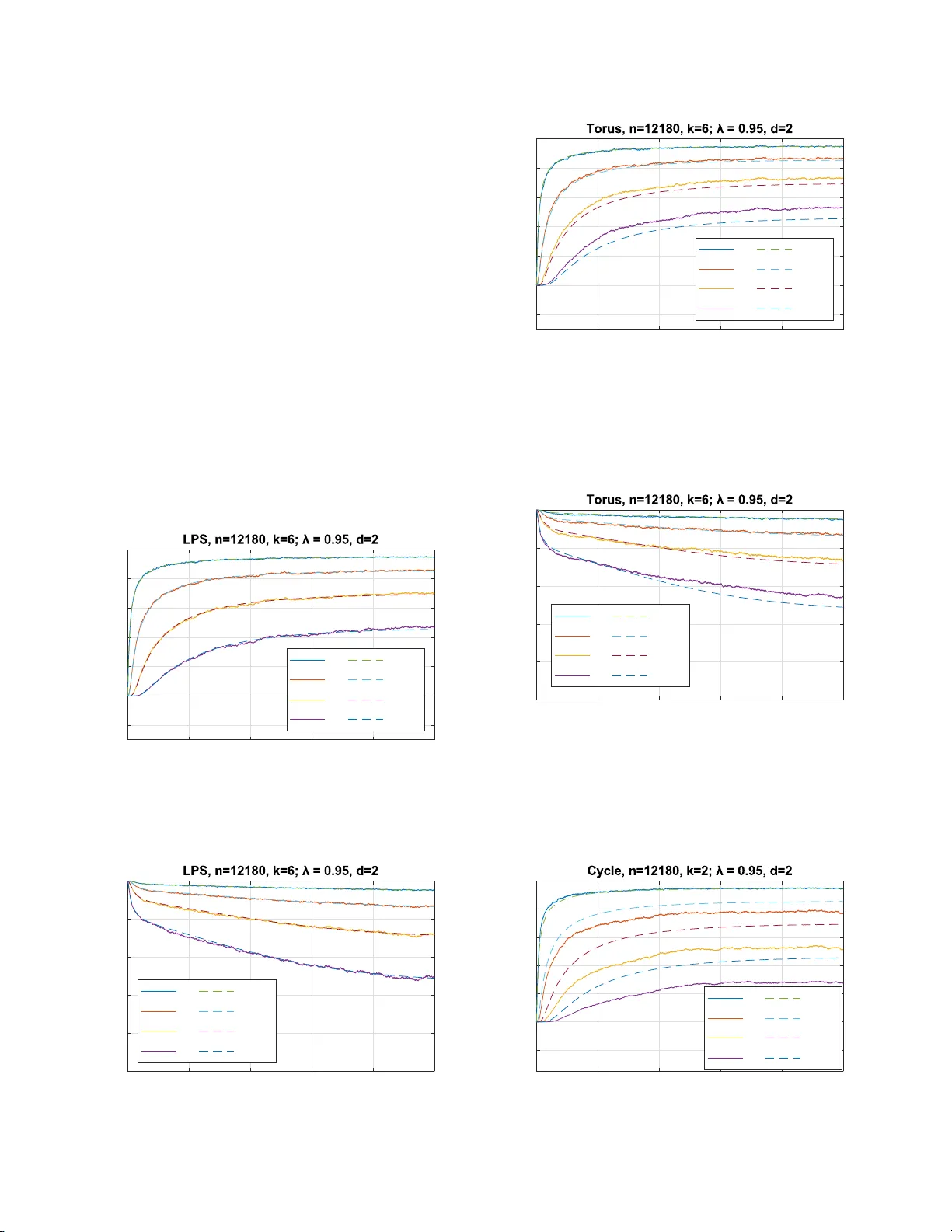
Derandomized Load Balanci ng using Random W alks on Expander Graphs Dengwang T ang a nd V ijay G. Subramanian University of Michigan, An n Arbor 1301 Beal A ve, Ann Arbor , Mich igan Email: {dwtang, v gsubram} @umich.edu Abstract —In a computing center with a large number of machines, when a job arriv es, a di sp atcher need t o decide w h ich machine t o route this job to b ased on l i mited information. A classical method, called the power-o f- d choices algorithm, i s to pick d serv ers i n dependen t l y at random and d ispatch the job to t he least l oaded ser ver amo ng the d servers. In this paper , we analyze a low-randomness v ariant of this dispatching scheme, where d queues are sampled through d independent non-backtracking random walks on a k -regular graph G . Un der certain assumptions on the graph G , w e sh ow that under this scheme, the dynamics of the queuing system con verges to the same deterministic ordinary d ifferential equation (ODE) system fo r the po wer-of- d choices scheme. W e also show that the system is stable under the proposed scheme, and the stationary distribution of the system con verges to the fixed p oint of the ODE system. I . I N T R O D U C T I O N In co m puting centers where an extrem e ly large am ount of computatio ns are perfo rmed, there are usu ally a m ultitude of servers. This enables the comp uting center to h andle multiple jobs at the same time. When a com putational job is given to a computin g center , a ro uter , o r a dispatc h er , d ecides on which server to s end the job to. The o b jectiv e of th e router is to minimize the queuing delay , hence enhancing the performan c e of the system. In several queu ing system setting s, it has been known that Join -the-Sho r test-Queue (JSQ) is an optima l dispatching policy [1]. However , it is not always pr actical to implement th is po licy , especially when the system contains a large number of servers, since JSQ requ ires the dispatcher to inq uire every server’ s queu e length, and a d ecision can only be made after all ser vers have returned the q u eue length informa tio n to the dispatcher . In spired by this challeng e, researchers have bee n analyz in g sch emes where the dispatcher only inq uire the queue len g th of a small su bset of servers [2]– [4]. It turns out that, in a large sy stem , the power-of-2-choices scheme [3], where the jo b is sent to the shorter qu e u e of 2 unifor m ly r andomly and independen tly chosen servers/queues, can r educe th e qu euing delay significantly when com p aring to the random assignment scheme; where a job is simply sent to a randomly cho sen server . T he an alysis is achieved through the m e th od of fluid limit estimation , where the evolution of the queu ing system is shown to be appr oximately following the solution to a system of or dinary differential equatio n s fo r large systems. This scheme is a lso extended to power-of- d - choices scheme where d servers a r e sampled for each job . The parameter d ≥ 2 can either be a constant or gr ow with the size of the system. Subsequ ent work has been prop osing and analyzing variants of the power-of- d -choices scheme. The authors of [ 5] pro posed a mo d el where the d ispatcher has memory which can sto r e the iden tity o f a sampled server . In this scheme, at each time the q ueue length s o f d rand omly sampled servers and th e server in the mem ory are co mpared ; the jo b joins the shorte st queu e among them, an d th e id entity of the shortest q u eue among the d rando m c h oices is sav ed in the memo ry for next job. Th e fluid limit a pprox imation re su lt for this sch eme is e stablished in [ 6]. Y ing et al. [7] extended the use of po wer -of- d -choices schem e to the case of batch job arrivals, where each arri val consists of k par allel tasks, slightly more than one server p er task are sampled and th e k tasks ar e a ssigned to the sampled servers in a water-filling manner . Mukher jee et al. [8] and Budh iraja et al. [9] a n alyzed a variant of power-of- d -choices where the servers are assum ed to be intercon n ected thr o ugh a high-d egree graph, and d ran dom servers are obtained by choo se a ran dom vertex and a subset of its neig hbors. Ganesh et al. [1 0] also utilized an un derlyin g graph to f or loa d balancing problem s, where jo bs can switch to other queues after a ssign ment. In the model of ball-in-bins, where m balls are placed into n bins sequentially accordin g to some po licy , and the b alls does n o t leav e the bins, the power- of- d -choices scheme and it s variants are also analyzed. See [11] for a list o f referenc e s. In m o st o f the papers discussed a b ove, the m odels assum e that th e sam p ling of servers for different jobs is perf ormed in an inde penden t manner, althou g h dependen ce of th e d servers sampled by the same job can b e present. Wh e n implem enting these mod e ls, Θ(log n ) bits o f randomness are requir e d for each jo b . True random ness is an impo rtant resou r ce on a computer, hen ce in many co mputer scien ce app lications, it is desirable to have a random ized a lg orithm which uses only a small amo unt of randomn ess. Rand om walks on expan der graphs have be en utilized to rep lace inde penden t unif o rm random ness in many random ized algorithms [12]. Alon et al. [13] analyzed the non-ba cktracking rand om walk (NBR W) on high g ir th expan der graph s. A ty pical NBR W sam ple p ath has se veral statistics that are s imilar to that of indepen dent u niform sampling. Motiv a te d by these works, we prop o sed the f ollow- ing variant of power-of- d -choices scheme: Assuming that the servers are in terconn ected by a k -regular grap h G , at each tim e a job arriv es at the system, d candida te servers are chosen by the location of d indep endent non-back tracking ran dom walkers, the jo b joins the shor test queue among the d queues of the ca n didate servers, and each ran dom walker moves indepen d ently to o ne of the k − 1 neigh bors and uniform ly at random . W e ref er to this sch e me as Non -backtrac kin g Rand om W alk based P ower-of- d -choices (NBR W -Po d ) scheme. In this paper, we an a lyze the NBR W - Po d scheme in the standard light tr affic model. The NBR W -Po d s cheme can be v iewed as a derando mized versio n of power-of- d -choices sche m e, since on e o f the results of this paper is th at it achiev es the same perfo rmance of power-of- d -choices while red ucing random ness. Our work in [11] is closely related to this work, as the same dispatching schem e ( NBR W -Po d ) is analyzed in the balls-in-bin s model. Wh ile the results in ball-in-bins m odel suggests that NBR W - Po d has a similar be haviour a s power- of- d -choices , it is not clear th at this is still tru e in the dy n amic queuing system setting s. Our work in [ 14] is also closely related to this work, where the Non-backtrac kin g Rando m W alk with Restart based P ower-of- d -choices (NBR WR-Po d ) scheme is analyzed . The key dif f e rence between the two works lies in two places. First, the rando m walkers in NBR WR-Po d [ 14] are p eriodically reset to independen t unifor m rando m po sitions, while the random walkers in NBR W -Po d , th e scheme in this paper, never reset. Secondly , the assumptions on the under lying graph f o r NBR WR-Po d [ 14] are weaker than that o f NBR W - Po d : NBR W -Po d r equires hig h-girth expander graph s, while NBR WR-Po d [14] r equires only hig h-girth graphs. W e charac terize the performance of NBR W - Po d schem e via the fo llowing results: 1) W e p rovide a fluid-limit appr oxima tion for the NBR W - Po d scheme in Sectio n IV -A, where the dynam ics of the queuing system up to a finite time T > 0 is shown to co n verge to the solution of a deterministic ordinar y differential equatio n ( ODE), which is the same O D E for the regular po wer-of- d choices [ 4 ] [3]. 2) W e show in Section IV -B that, the NBR W -Po d scheme stablizes the system under the assumption th at the under- lying gra p h G is co nnected and aperio dic. 3) W e show an inter change of lim its result in Sec tio n IV -C, which states that th e stationa r y d istribution of the queuing system unde r NBR W -Po d sch e me conver ges to the un ique fixed point of the lim iting ODE. 4) W e con d uct simu lations in Section V to sho w that th e ODE c a n be a g o od appr oximation for th e d ynamics of relativ ely small sy stems. W e also investigate the dyn a m- ics of the system under different un derlying g raphs to explore further the relationship b e tween graph family an d perfor mance o f the scheme. The proo f outline of ou r result are as follows: 1) Similar to [14], th e queu e length statistics process for the NBR W -Po d scheme is not a M a r kov Process, h ence the standard Kurtz’ s Theorem based fluid-limit appro xima- tion [15], [16] does not app ly . The metho ds o f W or mald [17] do esn’t apply either . Just as in [14], because of the use of r andom walks introdu ces de p endenc e on adjacent queues, we believe th at the pr opagation- of-chaos method, which was used by [18], cann ot be applied here. Sim ilar to [14], the proo f of the fluid- limit a p prox imation r e sult is based on martingale methods and Gr onwall lemma, where th e main difference to [14] is in the lac k of resets, which a llows for a similar decomp osition into a mar tingale compen sator with the co mpensator terms small b etween resets. A stronger character ization of the mixing pro perties of the r andom walk is th en used alo ng with mix ing times re placing the resets to achieve a similar decomp o sition. 2) For the stability result, our proo f utilizes a n ew v ariant of Foster-L y apunov Theorem which bou nds the “future one-step drift” of th e process. As in [14], the theorem is applied o n a sub p rocess an d then extend e d to the continuo us time process. 3) W e fo llow the techniq ue o f [7] to pr ove the conver - gence of station ary distributions, wher e f o r the unif orm tail bound p art, we u tilizes the new variant of Foster- L y apunov Theorem to provid e a bou n d. This paper is organized as follows: In Section I I we in- troduce our mod el and notations. In Section III we p rove a few preliminary results. In Sec tio n I V, we state an d prove our main results. W e provide simulation resu lts in Section V and conclud e in Section V I . I I . M O D E L In this pa per, we analyze the pro posed d ispatching scheme in the following standar d model: Th e r e are n servers in the system. E a ch server is associated with a q ueue. Jobs arrives a t the system following a Poisson process with rate λn , where λ < 1 is a constant. When a job arr ives at the system, the dispatcher s end the job to one of the servers. The services times for e ach jo b at each ser ver are i.i.d. exponential ran d om variables with m ean 1. The N BR W -Po d scheme is defined a s f ollowing: Assume that the servers are inter connected by a k -regu la r graph G = ([ n ] , E ) , wh ere k ≥ 3 is a constant. Let W 1 , W 2 , · · · , W d be d in depend ent non-backtr acking ran dom walks o n G . When the j -th jo b arriv es at the system, allocate the jo b to the least loaded ser ver among the servers W 1 { j } , · · · , W d { j } . Ties are broken arbitrarily . T o ensur e that the pro p osed scheme has goo d perfo r mance, we need the following a ssum ption on the graph G : Definition 1 (Ex pander Grap h) . [13] Let { G ( n ) } n be a sequence of k -regular graph s w ith n vertices. Let k = λ ( n ) 1 ≥ λ ( n ) 2 ≥ · · · ≥ λ ( n ) n be the eig en values of the ad jacency matrix of G ( n ) . Define λ ( n ) = max { λ ( n ) 2 , | λ ( n ) n |} . { G ( n ) } is called an λ -expander g raph sequence if the “second largest" eigenv alue λ ( n ) of the a d jacency matrice s of G ( n ) satisfies lim sup n →∞ λ ( n ) ≤ λ wher e λ is a constant satisfyin g λ < k . Assumption 1 ( G is a High Girth Ex pander ) . The graph sequence { G ( n ) } is a k -regular λ -expander gr aph sequ ence, and the girth of G ( n ) is g reater than 2 ⌈ α log k − 1 n ⌉ + 1 for sufficiently large n , w h ere α is a positive con stant. Remark 1. Such grap hs d o exist. For example, the seque n ce of Ramanujan graphs, called LPS graph s, in [19] is a sequence of ( p + 1) -r egu la r g r aphs satisfying Assumption 1 with α < 2 3 and λ = 2 √ p . By using a non-b acktrackin g random walk on high-girth graphs (instead of simp le random walks, or rand om walks on small girth grap hs), it is ensur ed that the ran d om walkers are not likely to revisit a vertex that it has recently v isited. This allows th e r andom walkers to find q u eues with relatively low load and h ence redu cing th e queu ing d e la y . It is kno wn that non- backtrack ing rand o m walks mix fas t on expander g raphs [1 3]. Comparing to the work in [14], th e fast mixing of NBR W -Po d play s the role o f resets in NBR WR-Po d [14], which ensure s that th e r andom walkers does not spend an extended time in a small subset of ser vers, hence ensuring that the server re sources are sufficiently used. A. Notation s n Number of servers, also the scaling paramet er for the system. G ( n ) A regular graph of n vertices. k Degre e of graph G ( n ) , which is a consta nt. Q ( n ) i ( t ) Queue length of s erve r i at (conti nuous) time t . Q ( n ) i [ j ] Queue length of s erve r i at the j -th ev ent (i.e. arri v al/pot entia l service) Q ( n ) i { j } Queue length of serve r i as seen by the j -th arriv al job X ( n ) i ( t ) Proportion of servers with load at least i at time t . W l { j } Position of the non-backtrac king random walk er l after j s teps of transition. W l { j } The directed edge that points to wards W l { j } from W l { j − 1 } T j Arri val time of the j -th job . τ j Inter -arri val time between the ( j − 1) -th and j -th job. F t A filtration that the random walk and queuing process are adapted to T ABLE I N O TA T I O N S I N T H I S PA P E R For th e ease of exposition, we will drop the super script ( n ) in the p r oofs when n is clear f rom context. Four different b r ackets are employed to indicate d ifferent time index systems: ( t ) is used for continuo us time; [ j ] indicates the time of the j -th arrival and poten tial service, or the j -th transition in a un iformized ch ain; { j } indicates the time of the j -th arriv al job; h j i indicates the tim e o f the j ⌊ c log n ⌋ - th arriv al. All notations in the p aper will follow T able I, with the exception of Section I II, where gener al lemm as are proved and notatio ns stan d s for g eneral processes an d variables. For simplicity of n otation, when X is a random variable, t is a constant, and A is an event, we use Pr( X ≥ t, A ) to represent Pr( { ω : X ( ω ) ≥ t } ∩ A ) . In this pap er , “ X d ∼ Y ” means that “ X and Y ha ve the same distribution. ” “ ⇒ " stands for weak conver gence, or convergence in distribution. d W 1 , k·k 1 stands fo r the W 1 W asserstein distance of measur es on a metric space where the metric is induced by the norm k · k 1 . I I I . P R E L I M I N A RY R E S U LT S F O R N B RW- P O d In this section, we will prove a few g eneral preliminary results for the proo f s of o ur main r esults. A. Lar ge Deviation Results The following re su lts will be some b asic conc e ntration inequalities that we will use. Lemma 1 (Bernstein) . Let { Z j } ∞ j =1 be a pr oce ss adap ted to the filtration {F j } ∞ j = − 1 . Let N > 0 be even. If 0 ≤ Z j ≤ B and E [ Z j |F j − 2 ] ≤ m a.s. for all j ≥ 1 , then for any λ ≥ 2 N m , we have Pr   N X j =1 Z j ≥ λ   ≤ 2 exp  − 3 λ 32 B  Pr oof. By th e Unio n Bound, we h av e Pr   N X j =1 Z j ≥ λ   ≤ Pr   N 2 X j =1 Z 2 j ≥ λ 2   + P r   N 2 X j =1 Z 2 j − 1 ≥ λ 2   Applying the Bernstein Inequ ality p roved in [ 11], we obtain that Pr   N 2 X j =1 Z 2 j ≥ λ 2   ≤ exp  − 3( λ/ 2) 16 B  = exp  − 3 λ 32 B  Pr   N 2 X j =1 Z 2 j − 1 ≥ λ 2   ≤ exp  − 3( λ/ 2) 16 B  = exp  − 3 λ 32 B  . Combining all th e above we prove the result. B. A P recise Estimate of Sa m p ling Pr oba b ility W e have a sharp er characteriza tio n of the mixin g prope rty from Alon et al. [13]. Lemma 2 . Let V ( n ) ( t ) be a n o n-ba cktrac king rando m walk on k -re gular λ -expander graph G ( n ) . Defin e P ( t ) u 1 ,v , u 0 := Pr( V ( n ) ( t + 1) = v | V ( n ) (0) = u 0 , V ( n ) (1) = u 1 ) . Then ther e exists a constant c > 0 (which o nly dep ends on λ and k ) such that for sufficiently lar ge n , max u 0 ,u 1 ,v ∈ G ( n )     P ( t ) u 1 ,v , u 0 − 1 n     ≤ 1 n 2 ∀ t ≥ ⌊ c log n ⌋ Pr oof. The proof utilizes the same ob servations as in [13]. The result her e stre n gthens Lem ma 5 in [11]. Let A ( t ) u,v denote the num ber of n o n-back tracking walks of leng th t fr om u to v . Let ˜ P ( t ) be th e t -step transition probab ility ma trix of a non- backtrack ing random walk, where the first step o f th e rando m walk is to a unif orm rando m neighbo r of th e starting vertex. W e h av e ˜ P ( t ) = A ( t ) k ( k − 1) t − 1 . From the proof of Le mma 5 in [11], we h av e th e estimate max u,v     ˜ P ( t ) u,v − 1 n     ≤ k − 1 k ( t + 1 ) β t + 1 k ( k − 1) ( t − 1) β t − 2 t ≥ 2 where 1 √ k − 1 < β < 1 is a constan t which dep ends on λ and k . W e imm e diately obtain max u,v     A ( t ) u,v − k ( k − 1) t − 1 n     ≤ ( t + 1 )[( k − 1) β ] t + ( t − 1)[( k − 1 ) β ] t − 2 t ≥ 2 Our precise estimate will be ba sed on the following obser- vation: L et A ( t ) u 1 ,v , u 0 denote the nu mber of non -backtrac king walks of len gth t from u 1 to v which av oid u 0 in the first step. By a counting argum ent, we establish A ( t ) u 1 ,v , u 0 = A ( t ) u 1 ,v − A ( t − 1) u 0 ,v , u 1 Applying the ab ove observation iter a ti vely , we o btain A ( t ) u 1 ,v , u 0 = A ( t ) u 1 ,v − A ( t − 1) u 0 ,v + A ( t − 2) u 1 ,v − A ( t − 3) u 0 ,v + · · · + ( − 1) t A (2) u b ,v + ( − 1) t +1 A (1) u 1 − b ,v , u b where b = 1 if t is even, and b = 0 otherw ise. W e have | ( − 1) t +1 A (1) u 1 − b ,v , u b | ≤ 1 , hen ce by the triangle inequality ,       A ( t ) u 1 ,v , u 0 − t − 2 X j =0 ( − 1) j k ( k − 1) t − 1 − j n       ≤ t − 2 X j =0     A ( t − j ) u b ( j ) ,v − k ( k − 1) t − 1 − j n     + 1 where b ( j ) = 1 if j is even, and b ( j ) = 0 otherwise. Hence we h av e max u 0 ,u 1 ,v       A ( t ) u 1 ,v , u 0 − t − 2 X j =0 ( − 1) j k ( k − 1) t − 1 − j n       ≤ t − 2 X j =0 ( t − j + 1)[( k − 1) β ] t − j + t − 2 X j =0 ( t − j − 1)[( k − 1) β ] t − j − 2 + 1 ≤ t [( k − 1 ) β ] t t − 2 X j =0  [( k − 1) β ] − j + [( k − 1) β ] − j − 2  + 1 ≤ t [( k − 1 ) β ] t t − 2 X j =0  ( √ k − 1 ) − j + ( √ k − 1 ) − j − 2  + 1 ≤ 2 t ( t − 1)[( k − 1) β ] t + 1 (1) W e compu te t − 2 X j =0 ( − 1) j k ( k − 1) t − 1 − j n = k ( k − 1) t − 1 n · 1 − ( − k + 1 ) − t +1 1 − ( − k + 1 ) − 1 = ( k − 1) t n [1 − ( − k + 1 ) − t +1 ] Denote P ( t ) u 1 ,v , u 0 = Pr( V ( n ) ( t + 1) = v | V ( n ) (0) = u 0 , V ( n ) (1) = u 1 ) . Di vidin g both sides of (1) by ( k − 1) t we obtain max u 0 ,u 1 ,v     P ( t ) u 1 ,v , u 0 − 1 − ( − k + 1 ) − t +1 n     ≤ 2 t ( t − 1) β t + ( k − 1 ) − t Therefo re max u 0 ,u 1 ,v     P ( t ) u 1 ,v , u 0 − 1 n     ≤ 2 t ( t − 1) β t + ( k − 1) − t +     ( − k + 1) − t +1 n     = 2 t ( t − 1) β t +  1 + 1 n  ( k − 1) − t +1 ≤ [2 t ( t − 1) + 2( k − 1 )] β t (Since β ≥ 1 k − 1 ) The rest o f the proof is similar to tha t of Lemm a 5 in [11]. Observe th at RHS of above is decre a sing in t fo r sufficiently large t . Pick c = − 3 log β and set τ = ⌊ c log n ⌋ , f or suffi ciently large n we have max u 0 ,u 1 ,v     P ( t ) u 1 ,v , u 0 − 1 n     ≤ [2 τ ( τ − 1) + 2( k − 1 )] β τ = O  (log n ) 2 n 3  ∀ t ≥ ⌊ c log n ⌋ Hence, for sufficiently large n , we h av e max u 0 ,u 1 ,v     P ( t ) u 1 ,v , u 0 − 1 n     ≤ 1 n 2 ∀ t ≥ ⌊ c log n ⌋ C. A V ariant of the F oster -Lyapunov Theorem The following extensions of th e Foster-L yapu nov Theorem will also b e used. Lemma 3. An irr educible Markov Chain { X j } j ∈ N is positive r ecu rrent if ther e e xists a function V : S 7→ R + , positive inte gers 1 ≤ L < K , and a fin ite set B ⊂ S satisfying the following con ditions: E[ V ( X k +1 )] < + ∞ whenever E[ V ( X k )] < + ∞ E[ V ( X k + K ) − V ( X k + L ) | X k = x ] ≤ − ǫ + A 1 B ( x ) ( 2 ) for some ǫ > 0 and A < + ∞ . Pr oof. WLOG, assume that the set B is n on-em pty . Let F k := σ ( X 0 , X 1 , · · · , X k ) . Define τ := inf { t ∈ N | X t ∈ B } . τ is a stopping time with respect to the filtration ( F t ) t ∈ N . Fix x 0 ∈ B . Start th e chain fro m X 0 = x 0 . W e have E[ V ( X 0 )] = V ( x 0 ) < + ∞ . By as sumption, we th en have E[ V ( X k )] < + ∞ for all k ∈ N . As a conseq uence, E[ V ( X l ) | F k ] < + ∞ a.s. for all l , k ∈ N . Using (2), we obtain E[ V ( X k + K ) | F k ] + ǫ ≤ E[ V ( X k + L ) | F k ] + A 1 B ( X k ) Multiply both sides by 1 { τ >k } , using the fact that 1 { τ >k } is F k -measurab le, we o btain E[ V ( X k + K ) 1 { τ >k } | F k ] + ǫ 1 { τ >k } ≤ E[ V ( X k + L ) 1 { τ >k } | F k ] + A 1 B ( X k ) 1 { τ >k } Using 1 { τ >k } ≥ 1 { τ >k + K − L } , and the fact that 1 B ( X k ) 1 { τ >k } = 1 { k =0 } , we have E[ V ( X k + K ) 1 { τ >k + K − L } | F k ] + ǫ 1 { τ >k } ≤ E[ V ( X k + L ) 1 { τ >k } | F k ] + A 1 { k =0 } T aking expectatio n of b oth sides, we obtain E[ V ( X k + K ) 1 { τ >k + K − L } ] + ǫ P r( τ > k ) ≤ E[ V ( X k + L ) 1 { τ >k } ] + A 1 { k =0 } Let m ∈ N , summin g b o th sides over k = 0 , 1 , · · · , m w e obtain m + K − L X k = K − L E[ V ( X k + L ) 1 { τ >k } ] + ǫ m X k =0 Pr( τ > k ) ≤ m X k =0 E[ V ( X k + L ) 1 { τ >k } ] + A Every term in the ab ove inequality is fin ite, henc e we can rearrang e the inequality to o btain ǫ m X k =0 Pr( τ > k ) ≤ A + K − L − 1 X k =0 E[ V ( X k + L ) 1 { τ >k } ] − m + K − L X k = m +1 E[ V ( X k + L ) 1 { τ >k } ] ≤ A + K − L − 1 X k =0 E[ V ( X k + L ) 1 { τ >k } ] where the last inequ ality is true since V ( x ) ≥ 0 f or all x ∈ S . T ake m → ∞ , we obtain ǫ E[ τ ] = ǫ ∞ X k =0 Pr( τ > k ) ≤ A + K − L − 1 X k =0 E[ V ( X k + L )] < + ∞ Hence starting from x 0 ∈ B , the expected h ittin g time o f B is finite. Using Lem ma 2.1.3 from [20] we conclud e that X j is positive recu rrent. Lemma 4 (Mo ment B ound) . Suppo se { X j } j ∈ N is positive r ecu rrent, V , f , g ar e non-n e g ative fu n ctions on S , 1 ≤ L < K , a nd supp ose E[ V ( X k +1 )] < + ∞ whenever E[ V ( X k )] < + ∞ E[ V ( X k + K ) − V ( X k + L ) | X k = x ] ≤ − f ( x ) + g ( x ) ∀ x ∈ S Let ˆ X have the same distribution a s the stationary distri- bution of { X j } j ∈ N . Then E[ f ( ˆ X )] ≤ E[ g ( ˆ X )] . Pr oof. Let F k := σ ( X 0 , X 1 , · · · , X k ) . Let x 0 ∈ S be fixed. Set X 0 ≡ x 0 . W e hav e E [ V ( X 0 )] = V ( x 0 ) < + ∞ . By assumption, we then hav e E [ V ( X k )] < + ∞ f or all k ∈ N . As a conseq u ence, E[ V ( X l ) | F k ] < + ∞ a.s. for all l , k ∈ N . Hen c e E[ V ( X k + K ) | F k ] + f ( X k ) ≤ E[ V ( X k + L ) | F k ] + g ( X k ) Let τ be any stopping time w .r .t. {F k } ∞ k =0 . Mu ltiply b o th sides by 1 { τ >k } , using th e fact that 1 { τ >k } is F k -measurab le, we obtain E[ V ( X k + K ) 1 { τ >k } | F k ] + f ( X k ) 1 { τ >k } ≤ E[ V ( X k + L ) 1 { τ >k } | F k ] + g ( X k ) 1 { τ >k } Using 1 { τ >k } ≥ 1 { τ >k + K − L } , we have E[ V ( X k + K ) 1 { τ >k + K − L } | F k ] + f ( X k ) 1 { τ >k } ≤ E[ V ( X k + L ) 1 { τ >k } | F k ] + g ( X k ) 1 { τ >k } T aking expectation of bo th sides, we obtain E[ V ( X k + K ) 1 { τ >k + K − L } ] + E[ f ( X k ) 1 { τ >k } ] ≤ E[ V ( X k + L ) 1 { τ >k } ] + E[ g ( X k ) 1 { τ >k } ] Let n ∈ N , sum m ing both sides over k = 0 , 1 , · · · , n we obtain n + K − L X k = K − L E[ V ( X k + L ) 1 { τ >k } ] + n X k =0 E  f ( X k ) 1 { τ >k }  ≤ n X k =0 E[ V ( X k + L ) 1 { τ >k } ] + n X k =0 E  g ( X k ) 1 { τ >k }  Every term in the ab ove inequality is fin ite, henc e we can rearrang e the inequality to o btain n X k =0 E  f ( X k ) 1 { τ >k }  ≤ n X k =0 E  g ( X k ) 1 { τ >k }  + K − L − 1 X k =0 E[ V ( X k + L ) 1 { τ >k } ] − m + K − L X k = m +1 E[ V ( X k + L ) 1 { τ >k } ] ≤ n X k =0 E  g ( X k ) 1 { τ >k }  + K − L − 1 X k =0 E[ V ( X k + L ) 1 { τ >k } ] where the last inequ ality is true sinc e V ( x ) ≥ 0 f or all x ∈ S . T ake n → ∞ , we obtain E " τ − 1 X k =0 f ( X k ) # ≤ E " τ − 1 X k =0 g ( X k ) # + K − L − 1 X k =0 E[ V ( X k + L )] Let T m be the time of th e m -th return to state x 0 . T m is a stopping time w .r . t. {F k } ∞ k =0 . Hence E " T m − 1 X k =0 f ( X k ) # ≤ E " T m − 1 X k =0 g ( X k ) # + K − L − 1 X k =0 E[ V ( X k + L )] Using the equality of time and statistical averages we hav e E " T m − 1 X k =0 f ( X k ) # = m E[ T 1 ]E[ f ( ˆ X )] E " T m − 1 X k =0 g ( X k ) # = m E[ T 1 ]E[ g ( ˆ X )] Hence we h av e m E[ T 1 ]E[ f ( ˆ X )] ≤ K − L − 1 X k =0 E[ V ( X k + L )] + m E [ T 1 ]E[ g ( ˆ X )] where P K − L − 1 k =0 E[ V ( X k + L )] < + ∞ . Dividing bo th sides by m E[ T 1 ] and let m → ∞ we obtain th e result. I V . M A I N R E S U LT S A. Fluid Limit Appr ox imation for NBRW - P o d In this section, we prove our first m ain result: th e queu - ing system dynamics under NBR W -Po d schem e for a large system can b e appro ximated by th e solution s to a system of d ifferential equations, which is the sam e ODE as that of power-of- d scheme. W e assume that G ( n ) satisfies assumption 1 thr o ugho ut this section. Theorem 1. Con sider the dynamic system x ( t ) ∈ [0 , 1] Z + described by the following d iffer ential equation s: d x i d t = λ ( x d i − 1 − x d i ) − ( x i − x i +1 ) i ≥ 1 x 0 ( t ) ≡ 1 (3) Let X ( n ) ( t ) = ( X ( n ) i ( t )) i ∈ Z + be an infinite d imensional vector , wher e X ( n ) i ( t ) is the pr o portion of qu eues with length exceeding (o r equa l to) i at time t . Suppo se th a t (a) Rand om walker s ar e initialized to indep endent uniform random positions. (b) Q ( n ) (0) is deterministic (c) lim n →∞ k X ( n ) (0) − x (0) k 1 = 0 (d) k x (0) k 1 < + ∞ then for every fi nite T > 0 lim n →∞ sup 0 ≤ t ≤ T k X ( n ) ( t ) − x ( t ) k 1 = 0 a.s. Pr oof of Theorem 1. For th e inequ alities w e proved in all the proof s in this section, the ineq uality shou ld be u nderstoo d as true for all sufficiently large n . If not explicitly s tated, then the threshold for sufficiently large n depen ds only o n the system parameters (i.e. d, k , α , and λ ). Let a , b : [0 , 1 ] Z + 7→ [0 , 1] Z + be defined as a i ( x ) = ( λ ( x d i − 1 − x d i ) i ≥ 1 0 i = 0 b i ( x ) = ( x i − x i +1 i ≥ 1 0 i = 0 Here a ( x ) + b ( x ) will be the mean field tr ansition rate f or power of d -schem e. Here, we separate the an alysis f o r arrival and dep arture p arts. Both a a nd b are Lipschitz co ntinuou s operator s with respect to ℓ 1 norm, where a has Lipschitz constant 2 λd an d b ha s Lipschitz con stant 2 . For i ≥ 1 , define A i ( t ) to be the total number of arriv al jobs that are d ispatched to a server with lo ad i − 1 (just before this arriv al) b e fore (including ) time t . Defin e A 0 ( t ) ≡ 0 . Also define B i ( t ) to be th e number of d eparture s f rom queues with load i (just before this departu r e) before (inclu ding) time t . Let A ( t ) , B ( t ) denote the corre sp onding in finite dime nsional vectors. W e have th e relation X ( t ) = X (0) + A ( t ) n − B ( t ) n Now , define M ( t ) = X ( t ) − X (0) − Z t 0 [ a ( X ( u )) − b ( X ( u ))]d u The idea of the proo f is to bou nd k M ( t ) k 1 and then apply Gronwall’ s lemma to b ound k X ( t ) − x ( t ) k 1 . W e write M ( t ) =  A ( t ) n − Z t 0 a ( X ( u ))d u  −  B ( t ) n − Z t 0 b ( X ( u ))d u  =: M a ( t ) − M b ( t ) where M a ( t ) is the “arriv a l part", an d M b ( t ) is the “service" part. W e will bou nd k M a ( t ) k 1 and k M b ( t ) k 1 separately . Now we define two auxiliary queuing processes ˜ Q + ( t ) and ˜ Q − ( t ) , which ar e c o upled with Q ( t ) . Recall that an altern a ti ve d escription of Q ( t ) is as follows: Q ( t ) can be obtained from a discrete-time process Q [ j ] along with holding times, where the holding times are i.i.d. exponentially distributed with mean 1 ( λ +1) n . The ev olutio n of Q [ j ] can be described as follows Q [ j + 1] = ( Q [ j ] + R [ j ](1 − Λ[ j ]) − S [ j ]Λ[ j ]) + where Λ[ j ] , j = 0 , 1 , 2 , · · · are i.i.d. Bernoulli random vari- ables with mean 1 λ +1 , S [ j ] are i.i.d. uniform ly distributed on { e i } n i =1 which indicates po tential ser vices, R [ j ] ∈ { e i } n i =1 are po tential arrivals to th e system. Note that { Λ[ j ] } ∞ j =0 and { S [ j ] } ∞ j =0 are mutually indepen dent, an d also independ ent of { Q [ j ′ ] } j j ′ =0 . In the discrete process, let ˜ T [ s ] be the arr iv al timestamp of the s -th job (i.e. the s -th timestamp such that Λ[ j ] = 0 .) Let c > 0 be a constant such th at Lemma 2 holds. Define ˜ Q + [0] = ˜ Q − [0] = Q [0] and ˜ Q + [ j + 1] =      Q [ j ] j = ˜ T [2 s ⌊ c lo g n ⌋ ] for some s ∈ Z + ( ˜ Q + [ j ] − S [ j ]Λ[ j ]) + otherwise ˜ Q − [ j +1] =      Q [ j ] j = ˜ T [(2 s + 1) ⌊ c log n ⌋ ] for some s ∈ Z + ( ˜ Q − [ j ] − S [ j ]Λ[ j ]) + otherwise Finally , we de fin e ˜ Q [ j ] =                ˜ Q − [ j ] ˜ T [2 s ⌊ c lo g n ⌋ ] ≤ j < ˜ T [(2 s + 1) ⌊ c log n ⌋ ] for some s ∈ N ˜ Q + [ j ] ˜ T [(2 s − 1) ⌊ c log n ⌋ ] ≤ j < ˜ T [2 s ⌊ c lo g n ⌋ ] for some s ∈ N ˜ Q − [ j ] j < ˜ T [ ⌊ c log n ⌋ ] Under this coupling , we h ave the following observation: Observation 1. Sup p ose that T j ≤ t < T j +1 , then if th e random walkers d o no t visit a verte x i within time [ T j − 1 , t ) , then ˜ Q i ( t ) = Q i ( t ) . Define ˜ X ( t ) by ˜ X i ( t ) = 1 n n X j =1 1 { ˜ Q j ( t ) ≥ i } i ∈ Z + Similarly , define ˜ X + ( t ) , ˜ X − ( t ) to be the pr oportio n vectors correspo n ding to ˜ Q + ( t ) and ˜ Q − ( t ) , respectively . W e fu rther define X ( t ) as f ollows: X ( t ) = ˜ X ( T j ) T j ≤ t < T j +1 where T j is the (con tin uous) time o f the j -th ar riv al. In other words, X ( t ) is o btained from samplin g and holdin g ˜ X ( t ) at arrival e vents. E ffecti vely , X ( t ) is a pro cess which accumulates services at arriv al times. W e write M a ( t ) =  A ( t ) n − Z t 0 a ( X ( u ))d u  + Z t 0 [ a ( X ( u )) − a ( ˜ X ( u ))]d u + Z t 0 [ a ( ˜ X ( u )) − a ( X ( u ))]d u =: M a, 1 ( t ) + M a, 2 ( t ) + M a, 3 ( t ) Since k X ( t ) − ˜ X ( t ) k 1 ≤ 1 n n X l =1 | Q l ( t ) − ˜ Q l ( t ) | = 1 n n X l =1 ( Q l ( t ) − ˜ Q l ( t )) ≤ 2 ⌊ c log n ⌋ n ∀ t ≥ 0 and a is 2 λd -Lipschitz, we c a n boun d k M a, 3 ( t ) k by k M a, 3 ( t ) k 1 ≤ Z t 0 2 λd 2 ⌊ c log n ⌋ n du = 2 λdt ⌊ c log n ⌋ n Hence, sup t ∈ [0 ,T ] k M a, 3 ( t ) k 1 ≤ 4 λdT ⌊ c log n ⌋ n Now we try to bou nd k M a, 2 ( t ) k 1 and k M a, 1 ( t ) k 1 . Let r > 1 be a constant that we ch o ose later . W e n ow intr oduce two high proba bility e vents A := { ther e are strictly less th an eλT n jo b arriv a ls before T } B := A ∩ { no que ue has accepted mor e than κ r L log n arriv al jo bs within the fir st ⌊ eλT n ⌋ a rriv als } where L = d  c log( k − 1) 2 α + 1  and κ r = max { 32 r 3 , 4 eλT + 1 } . Lemma 5. W e ha v e Pr( A c ) ≤ e − λnT , Pr( B c ) ≤ e − λnT + 2 dn − r +1 Pr oof. By Che rnoff bo und we k now that Pr( A c ) = Pr(Poisson( λnT ) ≥ eλnT ) ≤ e − seλnT exp( λnT ( e s − 1)) ∀ s > 0 , and then p icking s = 1 r esults in Pr( A c ) ≤ e − λnT Now we estimate the pro b ability of B c : I f B is no t true, then either A is not true, o r some q ueue is allo cated with more th an κ r d log n arriv al jobs while A is true . Let V i,l h j i denote th e n u mber of visits to q ueue i by the l -th r andom walker b etween (discrete) time [( j − 1) ⌊ c log n ⌋ , j ⌊ c log n ⌋ ) . Let ˜ L = c log( k − 1) 2 α + 1 . Beca u se of the girth assum ption, we have V i,l h j i ≤ ˜ L fo r all i, l , j . Let N be the smallest e ven number that is at least eλT n ⌊ c log n ⌋ . W e have Pr( B c ) ≤ Pr( A c ) + P r   ∃ i ∈ [ n ] , d X l =1 N X j =1 V i,l h j i ≥ κ r L log n   ≤ Pr( A c ) + n d P r   N X j =1 V 1 , 1 h j i ≥ κ r ˜ L log n   ≤ Pr( A c ) + n d P r   N X j =1 ˜ L 1 V 1 , 1 h j i > 0 ≥ κ r ˜ L log n   = Pr( A c ) + n d P r   N X j =1 1 V 1 , 1 h j i > 0 ≥ κ r log n   Let G j := F T j ⌊ c log n ⌋ for j ≥ 0 and G − 1 be the tr ivial σ - algebra. {G j } ∞ j = − 1 forms a filtration, and V 1 , 1 [ j ] is adap ted to {G j } ∞ j =1 . By Lemm a 2 and the Union bou nd we have E[ 1 V 1 , 1 h j i > 0 |G j − 2 ] ≤ ⌊ c log n ⌋  1 n + 1 n 2  ≤ 2 ⌊ c log n ⌋ n =: ˜ m Setting κ r = max { 32 r 3 , 4 eλT + 1 } , we have κ r log n ≥ 4 eλT lo g n + log n ≥ 4 eλT + 8 ⌊ c log n ⌋ n (for sufficiently large n that does not dep e nd on T ) = 2  eλT n ⌊ c log n ⌋ + 2  · 2 ⌊ c log n ⌋ n ≥ 2 N ˜ m Hence we ca n apply Lem ma 1 and o btain Pr   ⌊ N ⌋ X j =0 1 V i, 1 h j i > 0 ≥ κ r log n   ≤ 2 exp  − 3 κ r log n 32  ≤ 2 n − r Hence Pr( B c ) ≤ Pr( A c ) + n d P r   ⌊ N ⌋ X j =0 1 V 1 , 1 h j i > 0 ≥ κ r log n   ≤ e − λnT + 2 dn − r +1 Remark 2 . It is possible (using the techniques in [13]) to show that the arriv a l jobs accep ted by a single queue within the first ⌊ eλT n ⌋ arr ivals is boun d ed by O ( log n log log n ) with a sufficiently large probab ility . Howe ver, an O (log n ) boun d is enoug h fo r o ur pur pose. Lemma 6. Pr sup t ∈ [0 ,T ] k M a, 2 ( t ) k 1 ≥ 2 λdT ε 2 , A ! ≤ e (1 + λ ) λT n (1 + λ ) − nε 2 Pr oof. Sam e as the proof of Le m ma 3 in [14]. The rest of the proof is to b ound k M a, 1 ( t ) k 1 . T o ach iev e this goal, we first sample the continuous-time p rocess M a, 1 ( t ) at times T j ⌊ c log n ⌋ , the time of the j ⌊ c log n ⌋ -th job arriv al. Denote M a, 1 h j i := M a, 1 ( T j ⌊ c l og n ⌋− ) The key lemma for the p roof is stated as f ollows: Lemma 7. F or all i ≥ and j ≥ 0 , | E[ M a, 1 i h j + 1 i − M a, 1 i h j i|G j − 1 ] | ≤ 2 d ⌊ c log n ⌋ 2 n 1+ α Pr oof. For 0 ≤ s < ⌊ c log n ⌋ , define I i { j, s } to be the indicator of the ev ent that ( j ⌊ c lo g n ⌋ + s ) -th arrival is allo c a ted to a queue of load i − 1 . For ease of notation, define W l { j, s } := W l { j ⌊ c log n ⌋ + s } , T j,s := T j ⌊ c l og n ⌋ + s , τ j,s := τ j ⌊ c log n ⌋ + s . Recall that τ j is the inter-arri val time between job j − 1 and job j (wh e re τ 1 is defined to be the arriv al time of the first job .) Just as in [14], we h av e M a, 1 i h j + 1 i − M a, 1 i h j i = ⌊ c log n ⌋− 1 X s =0  1 n I i { j, s } − a i ( ˜ X ( T j,s )) τ j,s +1  (4) Define D j,s to be the ev ent that (at least) o ne of W 1 { j, s } , W 2 { j, s } , · · · , W d { j, s } that has been visited by (at least) one of th e random walkers at so m e timestamps ( j − 1) + ⌊ c log n ⌋ ≤ t < j ⌊ c log n ⌋ + s . Conditioned on D c j,s , by Observ ation 1 we h av e Q W l { j,s } ( T j,s − ) = ˜ Q W l { j,s } ( T j,s ) . If j is even, then ˜ Q W l { j,s } ( T j,s ) = ˜ Q − W l { j,s } ( T j,s ) , then we have E[ I i { j, s } | G j − 1 ] = Pr  min l =1 , ··· , d Q W l { j,s } ( T j,s − ) = i − 1    G j − 1  ≤ Pr  min l =1 , ··· , d Q W l { j,s } ( T j,s − ) = i − 1 , D c j,s    G j − 1  + P r( D j,s | G j − 1 ) = Pr  min l =1 , ··· , d ˜ Q − W l { j,s } ( T j,s ) = i − 1 , D c j,s    G j − 1  + P r( D j,s | G j − 1 ) ≤ Pr  min l =1 , ··· , d ˜ Q − W l { j,s } ( T j,s ) = i − 1    G j − 1  + P r( D j,s | G j − 1 ) Similarly we h av e a lower bound E[ I i { j, s } | G j − 1 ] = Pr  min l =1 , ··· , d Q W l { j,s } ( T j,s − ) = i − 1    G j − 1  ≥ Pr  min l =1 , ··· , d Q W l { j,s } ( T j,s − ) = i − 1 , D c j,s    G j − 1  ≥ Pr  min l =1 , ··· , d ˜ Q − W l { j,s } ( T j,s ) = i − 1    G j − 1  − P r( D j,s |G j − 1 ) Now , we take advantage of the fo llowing importan t o bser- vation: Observation 2. L et j ≥ 0 be even. Given G j − 1 , ˜ Q − ( T j,s ) 0 ≤ s ≤⌊ c log n ⌋ is cond itionally independen t of ( W { j, s } ) s ≥ 0 . The o bservation is true for j = 0 since ( ˜ Q − ( T 0 ,s )) 0 ≤ s< ⌊ c log n ⌋ is a result of applying p otential service schedules to ˜ Q ( T 0 , 0 ) , and the service schedules are indepen d ent of the rand om walker p ositions since the random walkers are initialized independ e n tly of the initial qu eue lengths. Recall that G − 1 is defin e d to be th e trivial σ -alg e bra. Hence the observation is stating that ( ˜ Q − ( T 0 ,s )) 0 ≤ s< ⌊ c log n ⌋ is indepe n dent o f ( W { 0 , s } ) s ≥ 0 For j = 2 , the ob servation is true since ( ˜ Q − ( T j,s )) 0 ≤ s< ⌊ c log n ⌋ is a re sult of apply ing potential service schedules to ˜ Q ( T j − 1 , 0 ) , where ˜ Q ( T j − 1 , 0 ) is G j − 1 - measurable and the servic e sch e d ules are conditio nally indepen d ent of the ran dom walker p ositions given G j − 1 . Using the ob servation, we c o nclude that ˜ Q ( T j,s ) is cond i- tionally inde p enden t of W { j, s } cond itio ning o n G j − 1 . By Lemm a 2, we have     Pr ( W l { j, s } = v | G j − 1 ) − 1 n     ≤ 1 n 2 ∀ v = 1 , · · · , n, ∀ s ≥ 0 for j ≥ 1 . Th e a b ove is also true for j = 0 since G j − 1 is the trivial σ -alg ebra and Pr( W l { j, s } = v ) = 1 n . Hence Pr  min l =1 , ··· ,d ˜ Q − W l { j,s } ( T j,s ) = i − 1    ˜ Q ( T j,s ) , G j − 1  = X v 1 , ··· ,v d ∈ [ n ] Pr  W l { j, s } = v l , ∀ l = 1 , · · · , d | ˜ Q ( T j,s ) , G j − 1  × 1 { min l =1 , ··· ,d ˜ Q − v l ( T j,s )= i − 1 } = X v 1 , ··· ,v d ∈ [ n ] Pr  W l { j, s } = v l , ∀ l = 1 , · · · , d | ˜ Q ( T j,s ) , G j − 1  × d Y l =1 1 { ˜ Q − v l ( T j,s ) ≥ i − 1 } − d Y l =1 1 { ˜ Q − v l ( T j,s ) ≥ i } ! = X v 1 , ··· ,v d ∈ [ n ] d Y l =1 Pr ( W l { j, s } = v l | G j − 1 ) × d Y l =1 1 { ˜ Q − v l ( T j,s ) ≥ i − 1 } − d Y l =1 1 { ˜ Q − v l ( T j,s ) ≥ i } ! ≤ X v l ∈ [ n ] 1 ≤ l ≤ d d Y l =1  1 n + 1 n 2  d Y l =1 1 { ˜ Q − v l ( T j,s ) ≥ i − 1 } − d Y l =1 1 { ˜ Q − v l ( T j,s ) ≥ i } ! =  1 n + 1 n 2  d X v l ∈ [ n ] 1 ≤ l ≤ d d Y l =1 1 { ˜ Q − v l ( T j,s ) ≥ i − 1 } − d Y l =1 1 { ˜ Q − v l ( T j,s ) ≥ i − 1 } ! =  1 n + 1 n 2  d d Y l =1 n X v = 1 1 { ˜ Q − v ( T j,s ) ≥ i − 1 } − d Y l =1 n X v = 1 1 { ˜ Q − v ( T j,s ) ≥ i } ! =  1 n + 1 n 2  d d Y l =1 ( n ˜ X − i − 1 ( T j,s )) − d Y l =1 ( n ˜ X − i ( T j,s )) ! =  1 + 1 n  d h ( ˜ X − i − 1 ( T j,s )) d − ( ˜ X − i ( T j,s )) d i Similarly , Pr  min l =1 , ··· , d ˜ Q − W l { j,s } ( T j,s ) = i − 1    ˜ Q ( T j,s ) , G j − 1  ≥  1 − 1 n  d h ( ˜ X − i − 1 ( T j,s )) d − ( ˜ X − i ( T j,s )) d i For suf ficien tly large n , we hav e (1 + 1 n ) d − 1 ≤ 3 d 2 n and (1 − 1 n ) d − 1 ≥ − 3 d 2 n , in which case we h ave ( ˜ X − i − 1 ( T j,s )) d − ( ˜ X − i ( T j,s )) d − 3 d 2 n ≤ Pr  min l =1 , ··· , d ˜ Q − W l { j,s } ( T j,s ) = i − 1    ˜ Q ( T j,s ) , G j − 1  ≤ ( ˜ X − i − 1 ( T j,s )) d − ( ˜ X − i ( T j,s )) d + 3 d 2 n W e then conclud e that E[ I i { j, s }|G j − 1 ] ≤ Pr  min 1 ≤ l ≤ d ˜ Q − W l { j,s } ( T j,s ) = i − 1    G j − 1  + P r( D j,s |G j − 1 ) = E  Pr  min 1 ≤ l ≤ d ˜ Q − W l { j,s } ( T j,s ) = i − 1    ˜ Q ( T j,s ) , G j − 1     G j − 1  + P r( D j,s |G j − 1 ) ≤ E h ( ˜ X − i − 1 ( T j,s )) d − ( ˜ X − i ( T j,s )) d    G j − 1 i + 3 d 2 n + P r( D j,s |G j − 1 ) = 1 λ E h a i ( ˜ X ( T j,s ))    G j − 1 i + 3 d 2 n + P r( D j,s |G j − 1 ) (5) and similarly E[ I i { j, s }|G j − 1 ] ≥ 1 λ E h a i ( ˜ X ( T j,s )) |G j − 1 i − 3 d 2 n − P r( D j,s |G j − 1 ) ( 6) By co nstruction ( ˜ X ( T j,s )) is indepen d ent o f τ j,s +1 condi- tioned o n G j − 1 . Recall th at τ j,s +1 is an in ter-arri val time of jobs with E [ τ j,s +1 ] = 1 λn . W e have E h a i ( ˜ X ( T j,s )) τ j,s +1 |G j − 1 i = 1 λn E h a i ( ˜ X ( T j,s )) |G j − 1 i (7) Combining (4), (5), (6), and ( 7 ) we have | E[ M a 1 i h j + 1 i − M i h j i|G j − 1 ] | ≤ ⌊ c log n ⌋− 1 X s =0     1 n E [ I i { j, s }|G j − 1 ] − E h a i ( ˜ X ( T j,s )) τ j,s +1 |G j − 1 i     ≤ ⌊ c log n ⌋− 1 X s =0  3 d 2 n 2 + 1 n Pr( D j,s |G j − 1 )  (8) for j ≥ 0 even. W ith a parallel argu ment (replacing ˜ X − by ˜ X + ), (8) is also true for j ≥ 0 odd. Claim 1. F or all j ≥ 0 , Pr( D j,s |G j − 1 ) ≤ d ( ⌊ c log n ⌋ + s ) n α + d ( d − 1 )( ⌊ c lo g n ⌋ + s )(1 + n − 1 ) n a.s. Giv en Claim 1, we have | E[ M a 1 i h j + 1 i − M i h j i|G j − 1 ] | ≤ ⌊ c log n ⌋− 1 X s =0  3 d 2 n 2 + d ( ⌊ c log n ⌋ + s ) n 1+ α + d ( d − 1 )( ⌊ c lo g n ⌋ + s )(1 + n − 1 ) n 2  ≤ d ⌊ c log n ⌋ n  3 2 n + 3 ⌊ c log n ⌋ 2 n α + 3( d − 1) ⌊ c log n ⌋ 2 n + 3( d − 1) ⌊ c lo g n ⌋ 2 n 2  ≤ d ⌊ c log n ⌋ n · 2 ⌊ c log n ⌋ n α (For sufficiently large n . No tice that α < 1 .) Pr oof of Claim. For j = 0 , by unio n bound we have Pr( D 0 ,s ) ≤ d X l =1 s X r =0 Pr( W l { 0 , r } = W l { 0 , s } ) + X l 1 6 = l 2 s X r =0 Pr( W l 1 { 0 , r } = W l 2 { 0 , s } ) = d s X r =0 Pr( W 1 { 0 , r } = W 1 { 0 , s } ) + d ( d − 1) s X r =0 Pr( W 1 { 0 , r } = W 2 { 0 , s } ) ≤ ds n α + d ( d − 1 ) s n For j ≥ 1 , by un ion bound we have Pr( D j,s |G j − 1 ) ≤ d X l =1 s X r = −⌊ c log n ⌋ Pr( W l { j, r } = W l { j, s }|G j − 1 ) + X l 1 6 = l 2 s X r = −⌊ c log n ⌋ Pr( W l 1 { j, r } = W l 2 { j, s }|G j − 1 ) = d s X r = −⌊ c log n ⌋ Pr( W 1 { j, r } = W 1 { j, s }|G j − 1 ) + d ( d − 1) s X r = −⌊ c log n ⌋ Pr( W 1 { j, r } = W 2 { j, s }|G j − 1 ) ≤ d ( ⌊ c log n ⌋ + s ) n α + d ( d − 1)( ⌊ c log n ⌋ + s )(1 + n − 1 ) n Lemma 7 states that M a, 1 h j i is v ery close to satisfying the co ndition o f Le m ma 9, except fo r a small compensator . The next Corollary applies concentratio n inequalities to bou nd | M a, 1 i ( t ) | for each i . Corollary 1 . Let N := min  m ∈ 2 Z : m ≥ eλT n ⌊ c log n ⌋  = Θ  n log n  δ := 2 dN ⌊ c log n ⌋ 2 n 1+ α = O  log n n α  K r := ⌊ c log n ⌋ n + r log n ( ⌊ c log n ⌋ + 1) λn = O  (log n ) 2 n  Then for sufficiently larg e n , Pr sup t ∈ [0 ,T ] | M a, 1 i ( t ) | ≥ ε 1 + K r + δ, A ! ≤ 4 exp  − ε 2 1 8 N K 2 r  + e N n − r holds for a ny ε 1 > 0 for a ll i ≥ 1 . Pr oof. W e first provide a lemm a on the tail b o und for sum of exponential random variables. Lemma 8. Let Z be the sum o f ⌊ c log n ⌋ independe n t expo- nential random variables with mean 1 λn , then Pr  Z ≥ r log n ( ⌊ c log n ⌋ + 1) λn  ≤ en − r Pr oof. Lemm a 12 in [14]. Define Z a, 1 i h j i := M a, 1 i h j + 1 i − M a, 1 i h j i = 1 n ⌊ c log n ⌋− 1 X s =0 I i { j, s } − ⌊ c log n ⌋− 1 X s =0 a i ( ˜ X ( T j,s )) τ j,s +1 Now , decom p ose M a, 1 i h j i = ˜ M a, 1 i h j i + ∆ a, 1 i h i i where ˜ M a, 1 i h j i := M a, 1 i h 0 i + j − 1 X l =0  Z a, 1 i h l i − E[ Z a, 1 i h l i|G l − 1 ]  and ∆ a, 1 i h j i = j − 1 X l =0  E[ Z a, 1 i h l i|G l − 1 ]  W e immediately have E[ ˜ M a, 1 i h j i|G j − 2 ] = ˜ M a, 1 i h j − 2 i and | ∆ a, 1 i h j i| ≤ j · 2 d ⌊ c log n ⌋ 2 n 1+ α Thus, sup 0 ≤ j ≤ N | M a, 1 i h j i| ≤ sup 0 ≤ j ≤ N | ˜ M a, 1 i h j i| + N · 2 d ⌊ c log n ⌋ 2 n 1+ α = sup 0 ≤ j ≤ N | ˜ M a, 1 i h j i| + δ ∀ j a.s. (9) Now we pr ovid e a b ound for the differences of ˜ M a, 1 i [ j ] . Notice that ˜ M a, 1 i h j + 1 i − ˜ M a, 1 i h j i = Z a, 1 i h j i − E[ Z a, 1 i h j i|G j − 1 ] W e know that − ⌊ c log n ⌋− 1 X s =0 τ j,s +1 ≤ Z a, 1 i h j i ≤ ⌊ c log n ⌋ n a.s. Hence, E[ Z a, 1 i h j i|G j − 1 ] ≥ E   − ⌊ c log n ⌋− 1 X s =0 τ j,s +1    G j − 1   = − ⌊ c log n ⌋ λn a.s. and E[ Z a, 1 i h j i|G j − 1 ] ≤ ⌊ c log n ⌋ n a.s. Hence | ˜ M a, 1 i h j + 1 i − ˜ M a, 1 i h j i| = | Z a, 1 i h j i − E[ Z a, 1 i h j i|G j − 1 ] | ≤ ⌊ c log n ⌋ n + ma x    ⌊ c log n ⌋− 1 X s =0 τ j,s +1 , ⌊ c log n ⌋ λn    Define C to be the event tha t ∀ 0 ≤ j < N , ⌊ c log n ⌋− 1 X s =0 τ j,s +1 ≤ r log n ( ⌊ c log n ⌋ + 1) λn Under C , we hav e | ˜ M a, 1 i h j + 1 i − ˜ M a, 1 i h j i| ≤ ⌊ c log n ⌋ n + r log n ( ⌊ c log n ⌋ +1) λn = K r . Lemma 9 (M odified Azuma-Ho effding) . Pr  max 0 ≤ j ≤ N    ˜ M a, 1 i h j i    ≥ ε, C  ≤ 4 exp  − ε 2 4 N K 2 r  Pr oof. Fix i . For the purp ose of expo sition, set ˜ Z j := ˜ M a, 1 i h j i − ˜ M a, 1 i h j − 1 i an d By the Union Bound, we have Pr max 0 ≤ j ≤ N      j X l =1 ˜ Z j      ≥ ε, C ! ≤ Pr   max 0 ≤ j ≤ N         ⌈ j / 2 ⌉ X l =1 ˜ Z 2 l       +       ⌈ j / 2 ⌉ X l =1 ˜ Z 2 l − 1         ≥ ε, C   ≤ Pr max 0 ≤ j ≤ N 2      j X l =1 ˜ Z 2 l      + max 0 ≤ j ≤ N 2      j X l =1 ˜ Z 2 l − 1      ≥ ε, C ! ≤ Pr max 0 ≤ j ≤ N 2      j X l =1 ˜ Z 2 l      ≥ ε 2 , C ! + P r max 0 ≤ j ≤ N 2      j X l =1 ˜ Z 2 l − 1      ≥ ε 2 , C ! . (10) W e know that { P 2 j l =1 ˜ Z 2 l } N j =0 is a martingale w .r .t. {F 2 j } . Using the decision tree construc tio n used in Lemm a 8 .2 of [21], one can construct ra n dom variables { Y j } N j =0 such tha t • { Y j } N j =0 is a martingale w .r . t. {F 2 j } • | Y j − Y j − 1 | ≤ K r • Y j = P 2 j l =1 ˜ Z 2 l under event C Note that Lem ma 8.2 of [21] is stated for finite state space random variables, but it ca n be easily gene ralized to our setting, wher e the distribution of ˜ Z 2 l is driven b y discrete ev ents (i.e. arriv als and services.) By Azuma-H o effding Inequality for Maxima (E q 3 .30 of [22]) Pr max 0 ≤ j ≤ N 2 | Y j − Y 0 | ≥ ε ! ≤ 2 exp − ε 2 2( N 2 K 2 r ) ! we have Pr max 0 ≤ j ≤ N 2      j X i =1 ˜ Z 2 j      ≥ ε 2 , C ! = Pr max 0 ≤ j ≤ N 2 | Y j − Y 0 | ≥ ε 2 , C ! ≤ 2 exp  ( ε/ 2) 2 N K 2 r  = 2 exp  ε 2 4 N K 2 r  . (11) For the same reason , Pr max 0 ≤ j ≤ N 2      j X i =1 ˜ Z 2 j − 1      ≥ ε 2 , C ! ≤ 2 exp  ε 2 4 N K 2 r  (12) Combining (10),(11), an d (12) we prove the r esult. Now we have Pr  sup 0 ≤ j ≤ N | ˜ M a, 1 i h j i| ≥ ε 1 , C  ≤ 4 exp  − ε 2 1 4 N K 2 r  Combining (9) we have Pr  sup 0 ≤ j ≤ N | M a, 1 i h j i| ≥ ε 1 + δ, C  ≤ 4 exp  − ε 2 1 4 N K 2 r  When C is tru e, we have that, f or any t suc h that T j, 0 ≤ t < T j +1 , 0 for some 0 ≤ j < N , | M a, 1 i ( t ) − M a, 1 i h j i| ≤ ⌊ c log n ⌋ n + ⌊ c log n ⌋− 1 X s =0 τ j,s +1 ≤ K r a.s. Hence Pr sup t ∈ [0 ,T N ⌊ c log n ⌋ ] | M a, 1 i ( t ) | ≥ ε 1 + K r + δ, C ! ≤ 4 exp  − ε 2 1 4 N K 2 r  Same as in [14], using Lem ma 8 an d the U n ion bou nd we can boun d Pr( C c ) ≤ eN n − r Finally , under event A , T := T N ⌊ c log n ⌋ ≥ T (since N ⌊ c log n ⌋ ≥ eλT n ). Th u s Pr sup t ∈ [0 ,T ] | M a, 1 i ( t ) | ≥ ε 1 + K r + δ, A ! ≤ Pr sup t ∈ [0 , T ] | M a, 1 i ( t ) | ≥ ε 1 + K r + δ, A ∩ C ! + P r( C c ) ≤ 4 exp  − ε 2 1 4 N K 2 r  + e N n − r Lemma 10. Let ρ > 0 be a ny constan t. S et b := ⌈ ( ρ + κ r L ) log n + L ⌉ = Θ(log n ) ϕ := 2 N ⌊ c log n ⌋  k x (0) k 1 + 1 ρ log n  d = Θ  n (log n ) d  Then Pr sup t ∈ [0 ,T ] ∞ X i = b +1 | M a, 1 i ( t ) | ≥ ϕ n + λT  k x (0) k 1 + 1 ρ log n + L  d , B ! ≤ 2 exp  − 3 ϕ 32 ⌊ c log n ⌋  Pr oof. By assumption, lim n →∞ k X ( n ) (0) − x (0) k 1 = 0 , h ence for sufficiently large n , we h av e 1 n n X i =1 Q ( n ) i (0) = k X ( n ) (0) k 1 ≤ k x (0) k 1 + 1 Recall that the event B is an event in wh ich th e numb er of jobs each queu e acc e pted in first ⌊ e λT n ⌋ a r riv als is u pper bound ed by κ r L log n . Under event B , the queues with length at least ( ρ + κ r L log n ) at any time before the ⌊ eλT n ⌋ -th arriv al m ust have an initial length of a t least ρ log n . Hence sup 0 ≤ j b ( t ) := P ∞ i = b +1 A i ( t ) to be the number o f arrivals dispatched to queues with len g th at least b befor e time t (Recall that A i ( t ) is the nu mber of arriv als d ispatched to queues with length equal to i − 1 before time t ) . Let ˜ A >b ( t ) be the n umber of arriv al job s that satisfy the f ollowing con ditions: • The job arr iv e s before time t • The a ssign ed q ueue h as length at least b (ju st befo re arriv al time) • Either this job is the m -th job where m < ⌊ c log n ⌋ , or if this job is the m -th job whe r e j ⌊ c log n ⌋ ≤ m < ( j + 1) ⌊ c log n ⌋ for some j ≥ 1 and X ⌈ ( ρ + κL ) log n ⌉ ( T ( j − 1) ⌊ c log n ⌋ − ) ≤ k x (0) k 1 + 1 ρ log n Denote ˜ A >b h j i := ˜ A >b ( T j ⌊ c l og n ⌋ − ) . Set b := ⌈ ( ρ + κL ) log n + L ⌉ . W e have E[ ˜ A >b h j + 1 i − ˜ A >b h j i | G j − 1 ] ≤ ⌊ c log n ⌋  1 + 1 n  d  k x (0) k 1 + 1 ρ log n  d W e fu rther have ˜ A >b h j + 1 i − ˜ A >b h j i ≤ ⌊ c log n ⌋ a.s. Set ϕ = 2 N ⌊ c log n ⌋  1 + 1 n  d  k x (0) k 1 + 1 ρ log n  d , using Bernstein’ s In e quality ( Lemma 1) we obtain Pr  ˜ A >b h N i ≥ ϕ  ≤ 2 exp  − 3 ϕ 32 ⌊ c log n ⌋  Under e vent B , we hav e A >b ( t ) = ˜ A >b ( t ) for t ∈ [0 , T ] , and T N ⌊ c log n ⌋ ≥ T (since N ⌊ c log n ⌋ ≥ eλT n ). Hence Pr sup t ∈ [0 ,T ] ∞ X i = b +1 A i ( t ) ≥ ϕ, B ! = Pr sup t ∈ [0 ,T ] A >b ( t ) ≥ ϕ, B ! ≤ Pr ( A >b h N i ≥ ϕ, B ) = Pr  ˜ A >b h N i ≥ ϕ, B  ≤ 2 exp  − 3 ϕ 32 ⌊ c log n ⌋  Under event B , we also have X b +1 ( t ) ≤ X ⌈ ρ log n + L ⌉ { 0 } ≤ k x (0) k 1 + 1 ρ log n + L ∀ t ∈ [0 , T ] which implies that sup t ∈ [0 ,T ] ∞ X i = b +1 Z t 0 a i ( X ( u ))d u ≤ sup t ∈ [0 ,T ] Z t 0 λ ( X b +1 ( u )) d d u ≤ λT  k x (0) k 1 + 1 ρ log n + L  d Then, applyin g union boun d w e obtain Pr sup t ∈ [0 ,T ] ∞ X i = b +1 | M a, 1 i ( t ) | ≥ ϕ n + λT  k x (0) k 1 + 1 ρ log n + L  d ! ≤ 2 exp  − 3 ϕ 32 ⌊ c log n ⌋  Corollary 2 . F or an y ε 1 > 0 , let ˜ ε 0 = b ( ε 1 + K r + δ ) + ϕ n + λT  k x (0) k 1 +1 ρ log n + L  d , we h ave Pr sup t ∈ [0 ,T ] k M a, 1 ( t ) k 1 ≥ ˜ ε 0 , B ! ≤ b  4 exp  − ε 2 1 4 N K 2 r  + e N n − 3  + 2 exp  − 3 ϕ 32 ⌊ c log n ⌋  Pr oof. Applica tio n of the U n ion bo und, similar to p roof of Corollary 2 in [14]. Now we have p rovided bo u nds for k M a, 1 ( t ) k 1 , k M a, 2 ( t ) k and k M a, 3 ( t ) k 1 . Combin e all the above, ap plying the Union bound , we o btain Pr  sup 0 ≤ t ≤ T k M a ( t ) k 1 ≥ ˜ ε 0 + 2 λdT ε 2 + 4 λdT ⌊ c log n ⌋ n , B  ≤ b  4 exp  − ε 2 1 4 N K 2 r  + e N n − r  + 2 exp  − 3 ϕ 32 ⌊ c log n ⌋  + e (1 + λ ) λT n (1 + λ ) − nε 2 Now we boun d k M b ( t ) k 1 . This part o f the proo f is nearly identical to that of [14], h ence Lemma 11. Pr  sup 0 ≤ t ≤ T k M b ( t ) k 1 ≥ bε 3 + ( e + 1) T ( k x (0) k 1 + 1 ) ρ log n + L , B  ≤ 2 b exp  − nT h  ε 3 T  + e x p  − nT k x (0) k 1 + 1 ρ log n + L  Pr oof. I dentical to that o f Lemm a 6 of [1 4] Now , define ε 0 := b ( ε 1 + K r + δ ) + ϕ n + λT  k x (0) k 1 + 1 ρ log n + L  d + 2 λdT ε 2 + 4 λdT ⌊ c log n ⌋ n + b ε 3 + ( e + 1) T ( k x (0) k 1 + 1 ) ρ log n + L Combining all th e above bo unds, we have Pr sup t ∈ [0 ,T ] k M ( t ) k 1 ≥ ε 0 ! ≤ Pr  sup 0 ≤ t ≤ T k M a ( t ) k 1 ≥ ˜ ε 0 + 2 λdT ε 2 + 4 λdT ⌊ c log n ⌋ n , B  + Pr  sup 0 ≤ t ≤ T k M b ( t ) k 1 ≥ bε 3 + ( e + 1) T ( k x (0) k 1 + 1 ) ρ log n + L , B  + Pr( B ) c ≤ b  4 exp  − ε 2 1 4 N K 2 r  + e N n − r  + 2 exp  − 3 ϕ 32 ⌊ c log n ⌋  + e (1 + λ ) λT n (1 + λ ) − nε 2 + 2 b exp  − nT h  ε 3 T  + e x p  − nT k x (0) k 1 + 1 ρ log n + L  + e − λnT + 2 dn − r +1 =: p 0 Recall that N = Θ( n log n ) , K = Θ( (log n ) 2 n ) , δ = Θ( log n n α ) , b = Θ(log n ) , ϕ = Θ( n (log n ) d ) . Select ε 1 = p 4( r − 1 ) N K r log n , ε 2 = r log(1+ λ ) log n n α , ε 3 = ( r − 1) q T log n n , using the fact that h ( t ) = t 2 2 + o ( t 2 ) , we finally h ave ε 0 = o (1) , p 0 = O  log n n r − 1  Choose r = 3 . The rest of th e proo f fin ishes with Gr onwall’ s lemma and the Borel-Cantelli Lemma in the same way as [1 4]. Corollary 3 . Suppo se tha t (a) ( Q ( n ) (0) , W (0)) is determin istic (b) lim n →∞ k X ( n ) (0) − x (0) k 1 = 0 (c) k x (0) k 1 < + ∞ then for every fi nite T > 0 lim n →∞ sup 0 ≤ t ≤ T k X ( n ) ( t ) − x ( t ) k 1 = 0 a.s. Pr oof. For a m oment, assume that W (0) is uniform random on ~ E d (i.e. r a n dom walkers are initialized to indepen dent unifor m random po sitions). Cho ose r = d + 3 in the proo f of Theor em 1. Then we obtain Pr sup t ∈ [0 ,T ] k M ( t ) k 1 ≥ ε 0 ! ≤ O  log n n d +2  For each w ∈ ~ E d , we have Pr sup t ∈ [0 ,T ] k M ( t ) k 1 ≥ ε 0 ! ≥ ( k n ) − d Pr sup t ∈ [0 ,T ] k M ( t ) k 1 ≥ ε 0    W (0) = w ! Hence Pr sup t ∈ [0 ,T ] k M ( t ) k 1 ≥ ε 0    W (0) = w ! ≤ O  log n n 2  The rest of the p roof finishes with Gronwall’ s lemma and the Borel-Cantelli Lemm a. Corollary 4. Let ( Q ( n ) (0) , W (0)) be arbitrarily rando m and corr ela ted. Suppo se that (a) X ( n ) (0) co n ver ges to Y (0) weakly in ([0 , 1] Z + , k · k 1 ) (b) k Y (0) k 1 < + ∞ a.s. then for every finite t > 0 , X ( n ) ( t ) con ver ges to Y ( t ) weakly in ([0 , 1] Z + , k · k 1 ) , wher e Y ( t ) is the state of the dyn a mic system (3) with random initial state x (0) d ∼ Y (0) Pr oof. k Y (0) k 1 < + ∞ a.s. means th a t Pr( Y ∈ ℓ 1 ([0 , 1])) = 1 . Since ℓ 1 ([0 , 1]) ⊂ [0 , 1 ] Z + is separable with respect to the k · k 1 metric, we conclud e th at Y h as sepa r able suppo r t. By the Skorokho d represen ta tio n theo rem, there exist a sequen ce of ra ndom vector ( ¨ X ( n ) (0)) an d a random vector ¨ Y (0 ) such that ¨ X ( n ) (0) d ∼ X ( n ) (0) , ¨ Y (0 ) d ∼ Y (0) and lim k →∞ k ¨ X ( n ) (0) − ¨ Y (0 ) k 1 k →∞ − − − − → 0 a.s. (13) Giv en ( ¨ X ( n ) (0)) n , construct the sequence ( ¨ Q ( n ) (0) , ¨ W ( n ) (0)) n such that ( ¨ Q ( n ) (0) , ¨ W ( n ) (0)) d ∼ ( Q ( n ) (0) , W ( n ) (0)) , accordin gly an on the same pro b ability space. Construct ( ¨ Q ( n ) ( t ) , ¨ W ( n ) ( t )) n such that ( ¨ Q ( n ) ( t ) , ¨ W ( n ) ( t )) ev olves i ndepen dently for each n . Applying Coro llar y 3 we have Pr  lim n →∞ sup 0 ≤ t ≤ T k ¨ X ( n ) ( t ) − ¨ Y ( t ) k 1 = 0    ( ¨ X ( n ) (0)) n  = 1 for ω ’ s such that ¨ X ( n ) (0)( ω ) converges in ℓ 1 to ¨ Y (0 )( ω ) an d k ¨ Y (0 )( ω ) k 1 < + ∞ . By (13), ¨ X ( n ) (0)( ω ) co n verges in ℓ 1 to ¨ Y (0)( ω ) and k ¨ Y (0 )( ω ) k 1 < + ∞ for almost all ω , hen ce we have Pr  lim n →∞ sup 0 ≤ t ≤ T k ¨ X ( n ) ( t ) − ¨ Y ( t ) k 1 = 0  = 1 (14) In particular, (14) implies that X ( n ) ( t ) n →∞ = = = ⇒ Y ( t ) for each finite t . B. Stab ility o f NBRW -P o d In th is section we will show that th e propo sed sche m e stablizes the qu euing system for every finite n . T o achieve this, we need some non-asympto tic assumption on the grap h G ( n ) . For this section , we only imp ose the following min imal assumption on the graph G : Assumption 2. G is con n ected and aperio dic. Theorem 2. The Markov Pr o cess ( Q ( t ) , W ( t )) is irr educible and positive r ecurrent, and hence Q ( t ) t →∞ = = = ⇒ ˆ Q fo r some ˆ Q . Recall fr om [14] that we have two down-samp led versions of the process Q ( t ) . If sam pled at arrivals an d po tential departur es: Q [ j + 1] = ( Q [ j ] + R [ j ](1 − Λ[ j ]) − S [ j ]Λ[ j ]) + If sampled at arriv als: Q { j + 1 } = ( Q { j } + R { j } − S { j } ) + Lemma 12 . ( Q { j } , W { j } ) is irr edu cible and positive r ecur- r ent. Pr oof. L et Ω = Z n + × ~ E d be th e state space of the Markov Chain ( Q { j } , W { j } ) . First, we n eed to sho w that ( Q { j } , W { j } ) is ir reducib le : Define P ( t ) ( q , w ; q ′ , w ′ ) := P r( Q { t } = q ′ , W { t } = w ′ | Q { 0 } = q , W { 0 } = w ) • For every q ∈ Z n + , w , w ′ ∈ ~ E d , ( q , w ′ ) is accessible from ( q , w ) : Since the graph is connected and aperiodic, the non-b a c ktracking r a ndom walk on G con verges to its stationa r y distribution: u niform on a ll directed edge s. Hence in p articular, there exist a time K such that Pr( W l { K } = w ′ l | W l { 0 } = w l ) > 0 ∀ l > 0 which implies that Pr( W { K } = w ′ | W { 0 } = w ) > 0 W ith po siti ve pro b ability , S { j } = R { j } f or all j = 0 , 1 , · · · , K − 1 (i.e. in K steps, all ass igned jobs ( R { j } ’ s) are immediately canc e le d by services ( S { j } ’ s)). Hen ce P ( K ) ( q , w ; q , w ′ ) > 0 • For every q ∈ Z n + , i ∈ [ n ] , w ∈ ~ E d , ( q + e i , w ) is accessible fr om ( q , w ) : Let w ′ be such that all of w ′ 1 , · · · , w ′ d are poin ting to wards vertex i . There exist K 1 >, K 2 > 0 such th a t Pr( W { K 1 } = w ′ | W { 0 } = w ) > 0 Pr( W { K 1 + K 2 } = w | W { K 1 } = w ′ ) > 0 W ith po siti ve pro b ability , S { j } = R { j } f or all j = 0 , 1 , · · · , K 1 − 1 , K 1 + 1 , · · · , K 1 + K 2 − 1 and S { K 1 } = 0 (i.e . in K 1 + K 2 steps, all assigned jo bs ar e immediately canceled o ut by services except the at the K 1 -th s tep, where an arr iv al is assigne d to server i ). W e conclu d e P ( K 1 + K 2 ) ( q , w ; q + e i , w ) > 0 • For e very i ∈ [ n ] , every q ∈ Z n + such that q i > 0 , w ∈ ~ E d , ( q − e i , w ) is accessible fr om ( q , w ) : Let K > 0 be such that Pr( W { K } = w | W { 0 } = w ) > 0 W ith positive p robab ility , S { 0 } = R { 0 } + e i , and S { j } = R { j } fo r all j = 1 , · · · , K − 1 (i. e. in K steps, all assigned jobs are immed iately can celed out by serv ices, and queu e i receives one extra serv ic e ). Hence P ( K ) ( q , w ; q − e i , w ) > 0 From the above argument, we see that every state in Ω is accessible from every other state. Hence the chain is irreducib le. Define a L yap unov f u nction V : Z n + 7→ R + V ( q ) := n X i =1 q 2 i Now , we compu te th e drif t. For any j ≥ 0 , V ( Q { j + 1 } ) − V ( Q { j } ) = n X i =1 [( Q i { j } + R i { j } − S i { j } ) 2 + − ( Q i { j } ) 2 ] ≤ n X i =1 [( Q i { j } + R i { j } − S i { j } ) 2 − ( Q i { j } ) 2 ] = 2 n X i =1 Q i { j } ( R i { j } − S i { j } ) + n X i =1 ( R i { j } − S i { j } ) 2 = − 2 n X i =1 Q i { j } S i { j } + n X i =1 ( S i { j } ) 2 + 2 Q i ∗ { j } + 1 − 2 S i ∗ { j } ≤ − 2 n X i =1 Q i { j } S i { j } + n X i =1 ( S i { j } ) 2 + 2 Q W 1 { j } { j } + 1 − 2 S i ∗ { j } where i ∗ is th e qu eue that the ( j + 1) -th job d ispatched to , i.e. R { j } = e i ∗ . By the co n struction of the scheme we k now that Q i ∗ { j } = min 1 ≤ l ≤ d Q W l { j } { j } Since the gr aph G is assumed to be conne cted and aperiod ic, the non-b acktrackin g random walk o n G is an irr e ducible and aperiodic Mar kov Chain. Let K ∈ N the mixing time of no n- backtrack ing random walk on the n vertex grap h in th e sen se that Pr( W ( n ) 1 { K + 1 } = v | W ( n ) 1 { 0 } = u 0 , W ( n ) 1 { 1 } = u 1 ) ≤ 1 + λ 2 λ · 1 n ∀ u 0 , u 1 , v ∈ G (15) W e have E[ V ( Q { K + 1 } ) − V ( Q { K } ) | Q { 0 } , W { 0 } ] ≤ − 2E " n X i =1 Q i { K } S i { K }    Q { 0 } , W { 0 } # + E " n X i =1 ( S i { K } ) 2    Q { 0 } , W { 0 } # + 2 E  Q W 1 { K } { K } | Q { 0 } , W { 0 }  + 1 − 2E [ S i ∗ { K } | Q { 0 } , W { 0 } ] = − 2 λn E " n X i =1 Q i { K }    Q { 0 } , W { 0 } # + n  1 λn + 2 ( λn ) 2  + 2 E  Q W 1 { K } { K } | Q { 0 } , W { 0 }  + 1 − 2 λn W e have E[ Q W 1 { K } { K } | Q { 0 } , W { 0 } ] ≤ E[ Q W 1 { K } { 0 } | Q { 0 } , W { 0 } ] + K ≤ 1 + λ 2 λ · 1 n n X i =1 Q i { 0 } + K Using the dynamics of Q i { j } and the fact th a t ( a ) + ≥ a we have n X i =1 Q i { K } ≥ n X i =1 Q i { 0 } + K − K − 1 X s =0 n X i =1 S i { s } Hence E " n X i =1 Q i { K }    Q { 0 } , W { 0 } # ≥ n X i =1 Q i { 0 } + K − E " K − 1 X s =0 n X i =1 S i { s }    Q { 0 } , W { 0 } # = n X i =1 Q i { 0 } + K − K n · 1 λn = n X i =1 Q i { 0 } −  1 λ − 1  K Combining the ab ove we h ave E[ V ( Q { K + 1 } ) − V ( Q { K } ) | Q { 0 } , W { 0 } ] ≤ − 2 λn " n X i =1 Q i { 0 } −  1 λ − 1  K # + n  1 λn + 2 ( λn ) 2  + 1 + λ λn n X i =1 Q i { 0 } + 2 K + 1 − 2 λn = − 1 − λ λn n X i =1 Q i { 0 } + 2 λn  1 λ − 1  K + 1 λ + 2 λ 2 n + 2 K + 1 − 2 λn := − 1 − λ λn n X i =1 Q i { 0 } + C Let B := ( ( q , w ) ∈ Ω | n X i =1 q i ≤ λn ( C + 1) 1 − λ ) B is a finite sub set of Ω . Then we have E[ V ( Q { K + 1 } ) − V ( Q { K } ) | Q { 0 } = q , W { 0 } = w ] ≤ − 1 + ( C + 1) 1 B ( q , w ) Furthermo re, we have V ( Q { j + 1 } ) = n X i =1 ( Q i { j } + R i { j } − S i { j } ) 2 + ≤ n X i =1 ( Q i { j } + 1) 2 = V ( Q { j } ) + 2 n X i =1 Q i { j } + n Hence E[ V ( Q { j + 1 } )] ≤ E[ V ( Q { j } )] + 2E " n X i =1 Q i { j } # + n ≤ E[ V ( Q { j } )] + 2 v u u t n E " n X i =1 ( Q i { j } ) 2 # + n (Cauchy-Sch wartz) = ( p E[ V ( Q { j } )] + √ n ) 2 Hence whenever E [ V ( Q { j } )] < + ∞ , we have E[ V ( Q { j + 1 } )] < + ∞ . Therefor e the two co nditions o f Lem ma 3 are checked. W e conclude that ( Q { j } , W { j } ) is irr e ducible and positive recurrent. Pr oof of Theorem 2. Using Lemm a 8 from [1 4] and the same argument as in [14], we can conclud e that ( Q [ j ] , W [ j ]) ∞ j =0 is irredu cible and po siti ve recurrent. The n , through stand ard arguments relating a contin uous time Markov Chain (CTMC) to its unifo rmized chain , the CTMC ( Q ( t ) , W ( t )) is positive recurren t. Hence Q ( t ) t →∞ = = = ⇒ ˆ Q for some rando m vector ˆ Q . C. Con ver gence of S tationary Distributions In this section, we will show that the station a ry distribution of q ueue len gths co n verges to the stationary solution of the differential equatio n as th e sy stem size grows. For th e results in this section, we impo se Assumptio n 1 on the gr aph sequenc e { G n } n . W e first p rovide a refined m oment boun d. Lemma 13. Let L := d  c log( k − 1) 2 α + 1  , we h ave lim sup n →∞ E " 1 n n X i =1 ˆ Q ( n ) i # ≤ 1 + λ + 2 λL 1 − λ Pr oof. Set K = ⌊ c log n ⌋ where c > 0 is a co nstant such that Lemma 2 is true, we h av e Pr( W ( n ) 1 { K + 1 } = v | W ( n ) 1 { 0 } = u 0 , W ( n ) 1 { 1 } = u 1 ) ≤ 1 n + 1 n 2 ∀ u 0 , u 1 , v ∈ G ( n ) For n ≥ 2 λ 1 − λ , we have 1 n + 1 n 2 ≤ 1 + λ 2 λ 1 n , hence K satisfies (1 5). Fr om the proof o f Lemma 12 we immedia te ly have E[ V ( Q { K + 1 } ) − V ( Q { K } ) | Q { 0 } , W { 0 } ] = − 2 λn E " n X i =1 Q i { K }    Q { 0 } , W { 0 } # + n  1 λn + 2 ( λn ) 2  + 2 E  Q W 1 { K } { K } | Q { 0 } , W { 0 }  + 1 − 2 λn (16) and E " n X i =1 Q i { K }    Q { 0 } , W { 0 } # ≥ n X i =1 Q i { 0 } −  1 λ − 1  K (17) T o o btain a constant mo m ent bou nd, we need a tighter u pper bound o f E  Q W 1 { K } { K } | Q { 0 } , W { 0 }  than in the proof of Lemm a 12. Notice that und er Assumption 1, any vertex cannot be visited b y the rando m walkers b y more than L := d  c log( k − 1) 2 α + 1  times within K = ⌊ c log n ⌋ timestamps. Hence E[ Q W 1 { K } { K } | Q { 0 } , W { 0 } ] ≤ E[ Q W 1 { K } { 0 } | Q { 0 } , W { 0 } ] + L ≤ 1 + λ 2 λ · 1 n n X i =1 Q i { 0 } + L (18) Combining (16)(17)(18) w e obtain the estimate E[ V ( Q { K + 1 } ) − V ( Q { K } ) | Q { 0 } , W { 0 } ] ≤ − 1 − λ λn n X i =1 Q i { 0 } + 2 λn  1 λ − 1  K + 1 λ + 2 λ 2 n + 2 L + 1 − 2 λn Notice that by P AST A, ˆ Q , defined as the station ary queue vecto r o f th e continuou s time p rocess ( Q ( t ) , W ( t )) , is also station ary with re sp ect to the Markov Chain ( Q { j } , W { j } ) . Define f ( q , w ) = 1 − λ λn P n i =1 q i , g ( q , w ) ≡ 2 λn  1 λ − 1  K + 1 λ + 2 λ 2 n + 2 L + 1 − 2 λn , then apply Lemma 4, we o b tain 1 − λ λ E " 1 n n X i =1 ˆ Q i # ≤ 2 λn  1 λ − 1  ⌊ c log n ⌋ + 1 λ + 2 λ 2 n + 2 L + 1 − 2 λn n →∞ − − − − → 1 + λ + 2 λL λ Multiplying both sides by λ 1 − λ we prove the result. Lemma 14. F or some n ∈ N , lim b →∞ sup n ≥ n E " ∞ X i = b +1 ˆ X ( n ) i # = 0 Pr oof. This p r oof is similar to th e proof of Lemm a 10 in [14]. Define a fu nction V b : Z n + 7→ R + V b ( q ) := n X i =1 v b ( q i ) := n X i =1 ( q i − b ) 2 + Same as [ 14], we h ave V b ( Q { K + 1 } ) − V b ( Q { K } ) ≤ − 2 n X i =1 ( Q i { K } − b ) + S i { K } + n X i =1 ( S i { K } ) 2 1 { Q i { K }≥ b } + 2 ( Q W 1 { K } − b ) + + (1 − 2 S i ∗ { K } ) 1 { Q i ∗ { K }≥ b } where i ∗ is th e queue that th e ( K + 1) -th job is dispatched to. Set K = ⌊ c log n ⌋ and let n ≥ 2 λ 1 − λ (such th at K satisfies Eq . (15)) . Recall th at a server can be visited by the random walkers fo r a t most L times. Hence 1 { Q i { 0 }≥ b − L } ≥ 1 { Q i { K }≥ b } . Therefo re E[ V b ( Q { K + 1 } ) − V b ( Q { K } ) | Q { 0 } , W { 0 } ] ≤ − 2 λn E " n X i =1 ( Q i { K } − b ) +    Q { 0 } , W { 0 } # +  1 λn + 2 λ 2 n 2  n X i =1 1 { Q i { 0 }≥ b − L } + 2 E  ( Q W 1 { K } − b ) + | Q { 0 } , W { 0 }  +  1 − 2 λn  E  1 { Q i ∗ { K }≥ b } | Q { 0 } , W { 0 }  Same as in [14], we h av e ( Q W 1 { K } { K } − b ) + ≤ ( Q W 1 { K } { 0 } − b ) + + L 1 { Q W 1 { K } { 0 }≥ b − L } Using the fact that K is a m ix ing time ( i.e. satisfies Eq. (15)), we have E[( Q W 1 { K } { K } − b ) + | Q { 0 } , W { 0 } ] ≤ E[( Q W 1 { K } { 0 } − b ) + | Q { 0 } , W { 0 } ] + L E[ 1 { Q W 1 { K } { 0 }≥ b − L } | Q { 0 } , W { 0 } ] ≤ 1 + λ 2 λ 1 n n X i =1 ( Q i { 0 } − b ) + + L · 1 + λ 2 λ 1 n n X i =1 1 { Q i { 0 }≥ b − L } Same as in [14], we h av e n X i =1 ( Q i { K } − b ) + ≥ n X i =1 ( Q i { 0 } − b ) + − n X i =1 K − 1 X s =0 S i { s } 1 { Q i { 0 }≥ b − L } Thus E " n X i =1 ( Q i { K } − b ) +    Q { 0 } , W { 0 } # ≥ n X i =1 ( Q i { 0 } − b ) + − K λn n X i =1 1 { Q i { 0 }≥ b − L } W e also have 1 { Q i ∗ { j }≥ b } ≤ 1 { Q W 1 { j } { j }≥ b } ≤ 1 { Q W 1 { j } { 0 }≥ b − L } Hence E[ 1 { Q i ∗ { j }≥ b } | Q { 0 } , W { 0 } ] ≤ E h 1 { Q W 1 { j } { 0 }≥ b − L } | Q { 0 } , W { 0 } i ≤ 1 + λ 2 λ 1 n n X i =1 1 { Q i { 0 }≥ b − L } Combining all th e above, fo r sufficiently large n we have E[ V b ( Q { K + 1 } ) − V b ( Q { K } ) | Q { 0 } , W { 0 } ] ≤ − 2 λn " n X i =1 ( Q i { 0 } − b ) + − K λn n X i =1 1 { Q i { 0 }≥ b − L } # +  1 λn + 2 λ 2 n 2  n X i =1 1 { Q i { 0 }≥ b − L } + 2 1 + λ 2 λ 1 n n X i =1 ( Q i { 0 } − b ) + + L · 1 + λ 2 λ 1 n n X i =1 1 { Q i { 0 }≥ b − L } ! +  1 − 2 λn  1 + λ 2 λ 1 n n X i =1 1 { Q i { 0 }≥ b − L } = − 1 − λ λ 1 n n X i =1 ( Q i { 0 } − b ) + +  2 K λ 2 n + 1 λ + 2 λ 2 n + (1 + λ ) L λ + 1 + λ 2 λ − 1 + λ λ 2 n  × 1 n n X i =1 1 { Q i { 0 }≥ b − L } Since ( Q { j } , W { j } ) is positiv e recu rrent with stationar y queue vector ˆ Q , app lying Lemma 4 w e obtain 1 − λ λ E " 1 n n X i =1 ( ˆ Q i { 0 } − b ) + # ≤  2 ⌊ c log n ⌋ λ 2 n + 1 λ + 2 λ 2 n + (1 + λ ) L λ + 1 + λ 2 λ − 1 + λ λ 2 n  × E " 1 n n X i =1 1 { ˆ Q i { 0 }≥ b − L } # which means tha t there exist a co nstant κ 5 such that f or sufficiently large n , E " 1 n n X i =1 ( ˆ Q i { 0 } − b ) + # ≤ κ 5 E " 1 n n X i =1 1 { ˆ Q i { 0 }≥ b − L } # ≤ κ 5 E " 1 n n X i =1 ˆ Q i b − L # = κ 5 b − L E " 1 n n X i =1 ˆ Q i # ∀ b > L By Lemma 13 w e know that there exist n 1 ∈ N such tha t E  1 n P n i =1 ˆ Q i  ≤ 1 + λ + 2 λL 1 − λ + 1 for all n ≥ n 1 . Hence, ther e exist n (which doe s not depend on b ), such that sup n ≥ n E " 1 n n X i =1 ( ˆ Q ( n ) i − b ) + # ≤ κ 5 b − L  1 + λ + 2 λL 1 − λ + 1  Observe th at ∞ X i = b +1 ˆ X ( n ) i = 1 n n X i =1 ( ˆ Q ( n ) i − b ) + W e conclu de lim b →∞ sup n ≥ n E " ∞ X i = b +1 ˆ X ( n ) i # = 0 The rest of the proo f follows from similar argum ent as th e proof of Th eorem 9 and Theo rem 10 in [7]. For co mpleteness, we includ e a proo f here. Lemma 15. Every subsequen ce of ( ˆ X ( n ) ) has a furth e r subsequen c e that conver ges in d W 1 , k·k 1 Pr oof. Nearly the same as proof of Corollary 5 in [14] (except that, the p roof here is simpler). Endow [0 , 1 ] Z + with the me tric ρ ( x , y ) = sup i ≥ 0 | x i − y i | i + 1 Under the metr ic ρ , [0 , 1] Z + is a com pact separable metric space. Any co llection of pro bability me a sures is trivially tigh t in ([0 , 1] Z + , ρ ) . By the Pro khorov Th eorem, ev ery subsequen ce of ( ˆ X ( n )) h as a fur ther subseq uence that con verges weak ly in ([0 , 1] Z + , ρ ) . By th e Skorokh od representatio n th eorem, th ere exist a sequen ce of random v ectors ( ¨ X ( n k ) ) such that ¨ X ( n k ) d ∼ ˆ X ( n k ) with ( ¨ X ( n k ) ) conv erges in ([0 , 1] Z + , ρ ) almost surely . Denote its almo st sure limit by Y . Claim 2. P ∞ i =1 E [ Y i ] < + ∞ Pr oof of Claim. By Fatou’ s Lemma, we have ∞ X i =1 Y i = ∞ X i =1 lim inf k →∞ ¨ X ( n k ) i ≤ lim inf k →∞ ∞ X i =1 ¨ X ( n k ) i a.s. (19) Again, by Fatou’ s Lem ma, we have E " lim inf k →∞ ∞ X i =1 ¨ X ( n k ) i # ≤ lim inf k →∞ E " ∞ X i =1 ¨ X ( n k ) i # (20) By Lemm a 13 we k now that lim inf k →∞ E " ∞ X i =1 ¨ X ( n k ) i # = lim inf k →∞ E " 1 n k n k X i =1 ˆ Q ( n k ) i # ≤ 1 + λ + 2 λL 1 − λ (21) Combining (19)(20)(21) w e have E " ∞ X i =1 Y i # ≤ 1 + λ + 2 λL 1 − λ For a ny ε > 0 , by Lemma 14 and Claim 2, th ere exist b ∈ Z + such that sup k : n k ≥ n E " ∞ X i = b +1 ¨ X ( n k ) i # ≤ ε 3 , E " ∞ X i = b +1 Y i # ≤ ε 3 which implies E " ∞ X i = b +1 | ¨ X ( n k ) i − Y i | # ≤ 2 ε 3 for all k such that n k ≥ n . Since ¨ X ( n k ) i − Y i conv erges to 0 a. s., and | ¨ X ( n k ) i − Y i | ≤ 2 a.s., by the Bounde d Convergence Th eorem we have lim k →∞ E " b X i =0 | ¨ X ( n k ) i − Y i | # = 0 Thus, for sufficiently large k , E " b X i =0 | ¨ X ( n k ) i − Y i | # ≤ ε 3 and E[ k ¨ X ( n k ) − Y k 1 ] = E " b X i =0 | ¨ X ( n k ) i − Y i | # + E " ∞ X i = b +1 | ¨ X ( n k ) i − Y i | # ≤ ε Hence, we established that lim k →∞ E h k ¨ X ( n k ) − Y k 1 i = 0 which implies that ˆ X ( n k ) conv erges to Y in d W 1 , k·k 1 Theorem 3. lim n →∞ E[ k ˆ X ( n ) − ˆ x k 1 ] = 0 , wher e ˆ x is the unique fixed poin t o f (3) . Pr oof. Let ( ˆ Q ( n ) , ˆ W ( n ) ) be a rand om vector who se distribu- tion is the stationar y distribution with respect to the n -server system. Set ( Q ( n ) (0) , W ( n ) (0)) d ∼ ( ˆ Q ( n ) , ˆ W ( n ) ) for every n . W e have ( Q ( n ) ( t ) , W ( n ) ( t )) d ∼ ( ˆ Q ( n ) , ˆ W ( n ) ) f or every n an d all t ≥ 0 . In particu lar , X ( n ) ( t ) d ∼ ˆ X ( n ) for all n and t ≥ 0 . Let ( ˆ X ( n k ) ) ∞ k =1 be a subsequence o f ( ˆ X ( n ) ) n that co n verges in d W 1 , k·k 1 . Denote its limit by Y . By the pro of of L e mma 15 we k now that E[ k Y k 1 ] < + ∞ , hence k Y k 1 < + ∞ a .s. By Corollar y 4, X ( n k ) ( t ) k →∞ = = = ⇒ Y ( t ) ∀ t ∈ R + where Y ( t ) is the state o f the lim itin g dy namical system (specified by the d ifferential eq uations in (3)) with initial state giv en by the r a ndom variable x (0) d ∼ Y . Since the weak limit of sequen ces of random vectors is unique, we ob ta in Y ( t ) d ∼ Y ∀ t ≥ 0 (22) It is proved in [3] that th e limiting d ynamics in (3) is global asy m ptotically stab le . For any x (0) ∈ ℓ 1 ([0 , 1]) , we have x ( t ) t →∞ − − − → ˆ x . Hence, we have lim t →∞ Y ( t ) = ˆ x a.s. (23) Combining (22) and (23), we have Y = ˆ x a.s. W e have proved that every subsequence of ( ˆ X ( n ) ) n which converges in d W 1 , k·k 1 conv erges weakly to ˆ x . Since the weak limit of a sequence of random vectors is unique, we co nclude that every subsequ ence of ( ˆ X ( n ) ) n which conv erges in d W 1 , k·k 1 conv erges to ˆ x . Since ˆ x is deterministic, we fur ther hav e this subsequ ence to conver ge to ˆ x in L 1 . Combining Lemma 15, we conclude tha t e very subsequence of ( ˆ X ( n ) ) n has a further subsequ ence th at converges to ˆ x in L 1 . Therefo re we con clude that ˆ X ( n ) conv erges to ˆ x in L 1 . V . S I M U L AT I O N R E S U LT S While the main results in the p a per suggests that th e queuin g system dynam ics con verges to the solution of an ODE as th e system size g o es to in finity , it is no t clear how well the ODE approx imates th e dy namics of the system f o r any finite number of servers. In this section, we provide simulatio n results to show that this app roximatio n is still accurate for systems of tens of thousands o f servers, wh ich is the same scale as today’ s cloud computin g centers. W e also provide results to sho w that, for some graphs th at are low-girth or non-expan d er , the ODE can fail to c apture the d ynamics of the system. W e use L PS graph [19] as the und erlying gr aph. Sp ecifically , we use a 6 -regular LPS g raph of n = 12 180 vertices. T he queue leng th statist ics of sin gle sample p aths ar e shown in Figure 1 and 2. The resu lts show that the fluid -limit appro xi- mation can b e accurate fo r relatively small systems. W e also test the scheme on sma ll gir th g raphs. Specifically , we choo se th e 6 -regular tor us g raph Z 15 × Z 28 × Z 29 as the underly ing graph. The evolution of the q u eue len gth statistics are shown in Fig ure 3 and 4. The results sho w that when Assumption 1 is v iolated, the ODE system m ay fail to capture the system d y namics. W e also test the schem e on cycle gr aphs, which are high girth non-expa n der gr aphs. Th e evolution of the queue length statistics are shown in Figure 5 and 6 . The results a g ain show that when Assumptio n 1 is violated, the ODE system may fail to capture the system d ynamics. Note th a t in [14], with the presence of r esets, a similar scheme still yields th e same perfor mance as power-of- d -choices . 0 20 40 60 80 100 timeline -0.2 0 0.2 0.4 0.6 0.8 1 Propotion of queues X 1 X 2 X 3 X 4 x 1 (ode) x 2 (ode) x 3 (ode) x 4 (ode) Fig. 1. Queue length statistics ev olutio n for NBR W -Po d algorithm with d = 2 and λ = 0 . 95 . System is empty at time 0 . 0 20 40 60 80 100 timeline 0 0.2 0.4 0.6 0.8 1 Propotion of queues X 1 X 2 X 3 X 4 x 1 (ode) x 2 (ode) x 3 (ode) x 4 (ode) Fig. 2. Queue length statistics ev olutio n for NBR W -Po d algorithm with d = 2 and λ = 0 . 95 . Each queue has a length of 5 at time 0 . 0 20 40 60 80 100 timeline -0.2 0 0.2 0.4 0.6 0.8 1 Propotion of queues X 1 X 2 X 3 X 4 x 1 (ode) x 2 (ode) x 3 (ode) x 4 (ode) Fig. 3. Q ueue length statisti cs e volution for N BR W -Po d algorith m with d = 2 and λ = 0 . 95 . System is empty at time 0 . 0 20 40 60 80 100 timeline 0 0.2 0.4 0.6 0.8 1 Propotion of queues X 1 X 2 X 3 X 4 x 1 (ode) x 2 (ode) x 3 (ode) x 4 (ode) Fig. 4. Q ueue length statisti cs e volution for N BR W -Po d algorith m with d = 2 and λ = 0 . 95 . Each queue has a length of 5 at time 0 . 0 20 40 60 80 100 timeline -0.2 0 0.2 0.4 0.6 0.8 1 Propotion of queues X 1 X 2 X 3 X 4 x 1 (ode) x 2 (ode) x 3 (ode) x 4 (ode) Fig. 5. Q ueue length statisti cs e volution for N BR W -Po d algorith m with d = 2 and λ = 0 . 95 . System is empty at time 0 . 0 20 40 60 80 100 timeline -0.2 0 0.2 0.4 0.6 0.8 1 Propotion of queues X 1 X 2 X 3 X 4 x 1 (ode) x 2 (ode) x 3 (ode) x 4 (ode) Fig. 6. Queue length statistics ev olutio n for NBR W -Po d algorithm with d = 2 and λ = 0 . 95 . Each queue has a length of 5 at time 0 . V I . C O N C L U S I O N S In th is paper we prop osed and an alyzed a low-rando m ness load b alancing scheme for mu lti-server systems. Th e new scheme modifies the sampling procedu re of the classical power-of- d -choices by r eplacing indep endent u niform sam- pling with non- backtrack ing random walks on h igh-gir th ex- pander grap hs. W e show that, like power-of- d -choices , the system d ynamics und er the new scheme can be approxim ated by the solution to a system of ODE. W e also sho w that the scheme stablizes th e system under mild assump tions. Finally , we show that the stationary qu eue length distribution of the system u n der the pro posed scheme is the same as th at of power-of- d -choices . W e conclude th at the new scheme is a derand o mization of power -of- d -choices as it achiev es the same perfor mance b y using less ra ndomn ess. There ar e a few future research direc tions suggested by th is paper . First, the per forman ce of NBR W - Po d sch e m e und er a heavy traffic mod el is of in terest. Secon dly , as the hig h-girth expander assumptio n can be too strong, it is worth ide ntifying weaker assumptions in wh ich the results in this paper s till holds. Finally , ana ly zing the structu re of th e limiting station - ary distribution o f queue len gths for NBR W - Po d scheme, in particular, if pr o pagation of chao s occurs or n ot , is of intere st. A C K N O W L E D G M E N T The au th ors would like acknowledge support by NSF via gra n ts AST -13 43381 , AST -151 6075, IIS-15388 27 and ECCS160836 1, and also Harsha Honap pa and Y ang Xiao f or early discussions. R E F E R E N C E S [1] G. Foschini and J. Salz, “ A basic dynamic routing problem and diffu- sion, ” IEEE Tr ansactions on Communicatio ns , vol. 26, no. 3, pp. 320– 327, 1978. [2] M. Mitzenmac her , “Load balanci ng and density dependent jump marko v processes, ” in IEEE Symposium on F oundations of Computer Science (FOCS) . IEEE, 1996, p. 213. [3] ——, “The po wer of two choices in randomize d load balanc ing, ” IEEE T ransactio ns on P arallel and Distribu ted Systems , vol. 12, no. 10, pp. 1094–1104, 2001. [4] N. D. Vv edenskaya, R. L . Dobrushi n, and F . I. Karpele vich, “Queueing system wit h select ion of the shorte st of two queues: An asymptotic approac h, ” Probl emy P eredac hi Informatsii , vol . 32, no. 1, pp. 20–34, 1996. [5] M. Mitzenmach er , B. Prabhakar , and D. Shah, “Load balanc ing with memory , ” in IEEE Symp osium on F oundations of Computer Scie nce (FOCS) . IEEE, 2002, p. 799. [6] M. Luczak and J. Norris, “ A veragi ng ove r fast varia bles in the fluid limit for markov chains: applic ation to the supermark et mode l with memory , ” The Annals of A pplied Pr obability , vol. 23, no. 3, pp. 957–986, 2013. [7] L. Y ing, R. Srikant, and X. Kang, “ The power of sli ghtly more than one sample in randomized load balanc ing, ” in Computer Communicat ions (INFOCOM), 2015 IEEE Conf er ence on . IEEE, 2015, pp. 1131–1139. [8] D. Mukherje e, S. C. Borst, J. S. va n L eeuw aarden, and P . A. Whiting, “Uni versality of po wer-of- d loa d bal ancin g in many -serve r systems, ” arXiv prepri nt arXiv:1612.00723 , 2016. [9] A. Budhiraja , D. Mukherjee, and R. W u, “Supermark et model on graphs, ” arXiv prepri nt arXiv:1712.07607 , 2017. [10] A. Ganesh, S. Lilientha l, D. Manjunath, A. Proutiere , and F . Simatos, “Load balanci ng via random loca l search in closed and open systems, ” in ACM SIGMETRICS P erformance Evaluation Revie w , vol. 38, no. 1. A CM, 2010, pp. 287–298. [11] D. T ang and V . G. Subramania n, “Balanc ed allocati on with random walk based sampling, ” arXiv preprint arXiv:18 10.02722 , 2018. [12] S. Hoory , N. Linial, and A. W igderson, “Expa nder graph s and their applic ations, ” Bulletin of the American Mathematical Socie ty , vol. 43, no. 4, pp. 439–561, 2006. [13] N. Alon, I. Benjamin i, E . Lubetzk y , and S. Sodin, “Non-backt racking random walks mix faster , ” Communic ations in Contempora ry Mat he- matics , vol. 9, no. 04, pp. 585–603, 2007. [14] D. T ang and V . G. Subramania n, “Random walk based sampling for load balanc ing in multi -serve r systems, ” in ACM SIGMETRICS P erformance Evaluati on Revie w . A CM, 2019, p. In press. [15] S. N. Ethier and T . G. Kurtz, Marko v pr ocesses: charact erization and con verg ence . John Wi ley & Sons, 2009, vol. 282. [16] M. Draief and L. Massouli, Epidemics and r umours in complex net- works . Cambridge Univ ersity Press, 2010. [17] N. C. W ormald, “Diff erenti al equations for random processes and random graphs, ” The annals of applied probab ility , vol. 5, no. 4, pp. 1217–1235, 1995. [18] A.-S. Sznitman, “T opics in propaga tion of chaos, ” in Ecole d’été de pr obabilités de Saint-Flo ur XIX—1989 . Springer , 1991, pp. 165–251. [19] A. Lubotzky , R. Phillips, and P . Sarnak, “Ramanujan graphs, ” Combi- natorica , vol. 8, no. 3, pp. 261–277, 1988. [20] B. Hajek, “Notes for ece 567 : Communication netw ork ana lysis, ” 2006. [21] F . Chung and L . Lu, “Concent ration inequalit ies and martingale inequal- ities: a survey , ” Interne t Mathematics , vol . 3, no. 1, pp. 79–127, 2006. [22] M. Habib, C. McDiarmid, J. Ramirez-Alfonsin , and B. Reed, Probab ilis- tic methods for al gorithmic discr ete mathematics . Springer Science & Business Media, 2013, vol. 16.