Analytic solutions to two quaternion attitude estimation problems

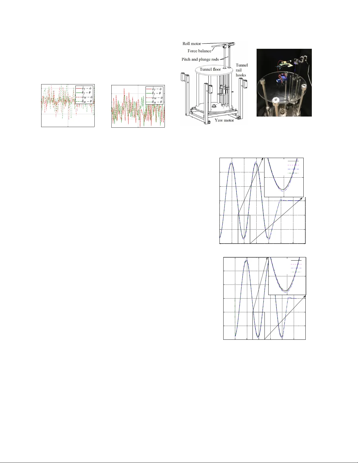
A unified geometric framew ork for rigid b o dy attitude estimation ? Y ujendra Mitikiri a , c Kamran Mohseni a , b , c a Dept of Me chanic al and A er osp ac e Engine ering, University of Florida, Gainesvil le, FL 32611 USA. b Dept of Ele ctric al and Computers Engine ering, University of Florida, Gainesvil le, FL 32611 USA. c Institute of Networke d Autonomous systems, University of Florida, Gainesvil le, FL 32611 USA. Abstract This paper presents solutions to the follo wing t w o common quaternion attitude estimation problems: (i) estimation of attitude using measuremen t of t wo reference v ectors, and (ii) estimation of attitude using rate measurement and measuremen t of a single reference v ector. Both of these problems yield to a direct geometric analysis and solution. The former problem already has a w ell established analytic solution in literature using linear algebraic metho ds. This pap er shows how the solution may also b e obtained using geometric metho ds, which are not only more in tuitive, but also amenable to uncon ven tional extensions b ey ond the traditional least-squares form ulations. With respect to the latter problem, existing solutions t ypically inv olve filters and observers and use a mix of differential-geometric and control systems metho ds. Again, this solution may also b e derived analytically using the geometric method, which helps impro v e the estimation accuracy . In this paper, b oth the problems are formulated as angle optimization problems, whic h can be solved to obtain a unique closed-form solution. The prop osed approac h has the fav ourable consequences that the estimation is (i) exact, th us ov ercoming errors in solutions based up on linear methods, (ii) instan taneous with respect to the measurements, thus o vercoming the latency inheren t in solutions based up on negativ e feedbac k upon an error, whic h can at best sho w asymptotic con vergence, and (iii) geometry-based, th us enabling imp osition of geometric inequalit y constrain ts. The geometric approac h has been v erified in sim ulations as w ell as experiments, and its performance compared against existing metho ds. Key wor ds: A ttitude estimation, geometric methods, quaternions, sensor fusion, nonlinear observers and filters. 1 In tro duction The problem of estimating the attitude of a rigid b o dy with resp ect to a reference co ordinate system, by mea- suring reference v ectors in a bo dy-fixed frame, has b een treated abundan tly in literature. One of the earliest, and arguably simplest, solution w as Blac k’s three-axis at- titude estimator TRIAD [7]. A least squares form ula- tion of the attitude estimation problem was p osed by W ah ba in [6]. Multiple solutions hav e b een rep orted for W ah ba’s problem: using p olar decomp osition [11], an SVD metho d, Dav enp ort’s q -metho d [10], the Quater- nion estimator QUEST [5], etc . Although b oth Dav enp ort’s q -metho d and QUEST use ? The authors would lik e to gratefully ackno wledge partial supp ort from the Air F orce Office of Scientific Researc h, and the National Science F oundation. Corresp onding author: Y ujendra Mitikiri. Email: yujendra@ufl.edu, Phone: (352) 273-2824. the quaternion represen tation of attitude, they ulti- mately reduce to an eigenv alue-eigenv ector problem. Th us it can b e seen that most solutions are linear al- gebraic in nature, and given the v ast array of to ols a v ailable for linear problems, they are all readily solv ed. This adv antage is, how ever, asso ciated with the ac- compan ying weakness that it is not straightforw ard to incorp orate nonlinear and nonholonomic constraints in the problem. F or instance, in [13], the authors describ e the attitude con trol of a spaceshuttle during a do c king op eration, when there is a hard constraint with respect to a nominal pitch angle in order to ensure that a tra- jectory control sensor is oriented to w ards the target platform. The attitude guidance mo dule then estimates an optimal pitch attitude that complies with the hard constrain t and minimizes the control effort. Similarly , in [19], the authors describ e a reference go v ernor with a p ointing inclusion constraint such that the spacecraft p oin ts to wards a fixed target, or an exclusion constrain t suc h that sensitive equipment is not exp osed to direct Preprin t submitted to Automatica 20 Decem b er 2024 solar radiation. Suc h inequalit y constraints are obvi- ously nonholonomic, and while b eing quite common in practice, are notoriously difficult to incorp orate in a linear algebraic solution. Once the guidance or refer- ence mo dule determines an attitude that complies with the constraints, a controller mo dule is used to achiev e b ounded or asymptotic stability with resp ect to the reference. Relatedly , the adven t of small unmanned v ehicles has motiv ated the developmen t of solutions that dep end up on minimal measuremen t resources in order to reduce the w eight and cost of the sensor pa yload. In particular, it is of considerable interest to estimate the attitude us- ing a single vector measurement, p ossibly supplemen ted b y a rate measuremen t, th us leading us to the second of the stated problems. This interest is partly fueled by the a v ailabilit y of c heap commercial-off-the-shelf inertial measuremen t units (IMUs) that contain MEMS-based gyroscop es and accelerometers [18]. The researc h is also partly fueled b y the realization that attitude estimation and control is a key c hallenge in the design of small autonomous aerial rob ots. The second problem is most frequently solved using an extended Kalman filter (EKF) [4]. The EKF provides a p oin t-wise attitude estimate and is instantaneous with resp ect to the measurements. How ever, resulting from linearization of an intrinsically nonlinear problem, this solution is not robust to large changes in the attitude state [9]. More recently , some solutions hav e b een rep orted in lit- erature which use nonlinear observers or filters to solve the single-vector measuremen t problem [9], [2], [16], [8], [15]. These solutions hav e typically used an appropriate error signal in negative feedback to estimate the atti- tude. The solutions in [9], and [16] are quite general, and while having b een dev elop ed for m ultiple vector mea- suremen ts, they extend smo othly to the case of a single v ector measuremen t. The solutions presen ted in [8], and [15] are more sp ecific to the av ailability of single vector measuremen ts. A common characteristic in this group of solutions is the use of negative feedbac k from an error sig- nal to estimate the attitude and an (a-priori) unknown gain, that needs to b e tuned in order to achiev e satis- factory estimator p erformance. Such a feedbac k-based estimator is b ound to hav e a finite latency with resp ect to the input, and cannot instan taneously track abrupt or discontin uous changes in the measuremen ts, and the con v ergence of the estimate to the true attitude is at b est asymptotic. In contrast to the linear algebraic and filter approac hes a v ailable in literature, this pap er analyzes the attitude estimation problems from a geometric p ersp ective. In the pro cess, we obtain solutions that ov ercome some of the shortcomings in the previous solutions. Firstly , b e- ing of a geometric nature, the solutions easily extend to problems in volving geometric constraints, irrespec- tiv e of whether they are holonomic equations or non- holonomic inequalit y constrain ts. Secondly , the analytic solutions provide an instan taneous estimate for the atti- tude whic h is consistent with resp ect to the v ector mea- suremen t at every time step. Besides the mathematical elegance of having an analytic solution, this also has sev- eral applications in autonomous guidance, navigation, and con trol systems: it enables the deplo yment of frugal single-v ector-measuremen t sensor-suites, and the zero- latency accuracy of the solution is useful in m ultiple- v ector-measuremen t suites in o v ercoming sudden fail- ures or intermitten t losses in some of the com p onen ts without leading to large transien t errors that could po- ten tially cause system breakdown. A brief outline of the paper is as follows. W e b egin by in- tro ducing the geometric approac h and formulating the stated problems in the language of mathematics in sec- tion 2. The next section, section 3.1, presen ts the solu- tion to the first problem, and relates it to the existing solutions from literature. The next section, Section 3.2, solv es the second problem and also provides results re- lating to the accuracy of the solution. A filtering metho d is introduced in section 3.3 to address the issue of mea- suremen t noise. This is follow ed by v erification of the theory using simulations and exp eriment in sections 5 and 6. 2 Notation, definitions, and problem formula- tion In this section, we describ e the geometry asso ciated with v ector measurements and formulate the attitude estima- tion problems as well-posed mathematical problems. The attitude of the rigid b o dy with resp ect to a ref- erence co ordinate system shall b e represented using a unit quaternion, denoted using a chec k accent, e.g. ˇ p = [ p 0 p 1 p 2 p 3 ] T , ˇ q = [ q 0 q 1 q 2 q 3 ] T . . . , such that ˇ p T ˇ p = ˇ q T ˇ q = . . . = 1, so ˇ p, ˇ q ∈ S 3 , the unit 3-sphere. The quaternion comp onents are related to the axis-angle rep- resen tation of a rotation by the relation q 0 = cos Φ / 2, and [ q 1 q 2 q 3 ] T = n sin Φ / 2, for a rotation through Φ ab out the axis n . The pro duct of tw o quaternions ˇ q and ˇ p shall b e denoted as ˇ q ⊗ ˇ p . W e shall follow the quater- nion algebraic conv entions describ ed in [20] chapter 11. A reference v ector, denoted in b old as h , k , . . . , shall b e defined as a unit magnitude v ector that p oints in a sp ec- ified direction. Examples include the direction of fixed stars relative to the bo dy , the Earth’s magnetic field, gra vitational field etc . The components of any suc h v ec- tor may b e measured in any three-dimensional orthog- onal co ordinate system. In the context of our problems, t w o obvious choices for the co ordinate system are the reference co ordinate system (relative to which the rigid b o dy’s attitude is to b e determined), and a co ordinate 2 system fixed in the bo dy . W e assume the a v ailability of measuremen t apparatus to obtain the vector’s comp o- nen ts in a three-dimensional orthogonal co ordinate sys- tem, g , h, . . . , a, b, . . . ∈ S 2 ⊂ R 3 in the reference and b o dy-fixed frames. A rotation quaternion (or, for that matter, any rotation represen tation) has three scalar degrees of freedom. A b o dy-referred measuremen t b of a reference vector has 3 scalar comp onents, that are related to the reference mea- suremen t h , in terms of the rotation quaternion. How- ev er, we also kno w that the measuremen t would retain the magnitude of the vector, i.e. , h T h = b T b = 1, so there is one scalar degree of redundancy in our measure- men t b and only tw o scalar degrees of information. Rec- onciling with this redundancy , we can therefore isolate the quaternion from a three-dimensional set of p ossibil- ities to a single-dimensional set. The redundancy can b e visualized as shown in figure 1. The measurement of a single vector in b o dy-fixed axes confines the b o dy’s attitude to form a conical solid of rev olution ab out h : those and only those attitudes on the cone would yield the same comp onents b . W e shall refer to the set of attitude quaternions consisten t with a measuremen t as the “feasibility cone” Q b corresp onding to that measurement b , i.e. , the measurement confines the attitude quaternion ˇ q to lie in Q b . F rom the previous discussion, Q b is one-dimensional and ˇ q has effectively a single degree of freedom. W e shall rep eatedly draw in tuition from the geometry in figure 1 to guide us in the solutions to the stated problems. Fig. 1. Possible attitudes of a minimal rigid b o dy formed out of three non collinear p oin ts (represented by the triangular patc h) consistent with a measurement of a single vector h . The subspace is a cone of revolution ab out the vector b eing measured. 2.1 Pr oblem 1. Estimation using me asur ements of two r efer enc e ve ctors Let the comp onen ts of tw o vectors h and k b e a = [ a 1 a 2 a 3 ] T and b = [ b 1 b 2 b 3 ] T in the b o dy co ordinate system, and h = [ h 1 h 2 h 3 ] T and k = [ k 1 k 2 k 3 ] T in the reference co ordinate system resp ectively . As describ ed ab o v e, each reference vector measurement provides tw o scalar degrees of information regarding the attitude of the rigid b o dy . It is immediately clear that the problem is ov erconstrained, and we ha ve more equations than unkno wns. Geometrically , w e hav e tw o feasibilit y cones Q a and P b , with the b o dy-axes intersecting along tw o lines, but with different roll angles for the b o dy ab out the b o dy-axis. Th us there is no exact solution to this problem in general, unless some of the measurement in- formation is redundant or discarded. A trivial means to w ell-p ose the problem is to discard comp onen ts of one of the vector, say k , along the sec- ond, h . This is exactly what is done with the TRIAD solution [7], where we use the orthogonal vector triad h , h × k , and h × ( h × k ) to determine the attitude. A more sophisticated approac h is to use all the measure- men t information – four scalar degrees of information with tw o reference vector measuremen ts –, and frame the problem as a constrained four-dimensional optimization problem in terms of the quaternion comp onents. This leads to Da venport’s q -metho d and QUEST solutions to W ah ba’s problem [6]. A no vel third approac h presented in this pap er, is to first determine tw o solutions ˇ q and ˇ p , one each lying on eac h of the feasibilit y cones Q a and P b corresp onding to the measurements a and b , and “closest” to the other cone in some sense. W e then fuse the estimates ˇ q and ˇ p appropriately to obtain the final attitude estimate. F or example, the final estimate could b e obtained using lin- ear spherical interpolation, and the w eights b e c hosen to represen t the relativ e significance attached to the indi- vidual measurements. The first problem can therefore b e stated as: given the me asur ements a and b in a r otate d c o or dinate system, of the two r efer enc e ve ctors h and k , we would like to estimate the r otate d system’s two attitude quaternions ˇ q ∈ Q a closest (in the le ast squar es sense) to P b and ˇ p ∈ P b closest (in the le ast squar es sense) to Q a , wher e Q a and P b ar e the r esp e ctive fe asibility c ones . 2.2 Pr oblem 2. Estimation using r ate me asur ement and me asur ement of single ve ctor Supp ose we ha v e a measuremen t of the comp onents ω = [ ω 1 ω 2 ω 3 ] T of the angular v elo city ω of a mo ving rigid b o dy , and that we also ha ve a measurement of the com- p onen ts b = [ b 1 b 2 b 3 ] T of a reference vector h , both measuremen ts b eing made in the b o dy co ordinate sys- tem. The comp onents of h in the reference co ordinate system are also known, say h = [ h 1 h 2 h 3 ] T . The prob- lem is to make a “b est” estimate of the b o dy’s attitude ˇ q on the basis of the pair of measurements ω and b , and kno wing h . 3 W e shall assume that the initial attitude quaternion is determined using, for e.g. , a solution to the first prob- lem or by some other means TRIAD, QUEST, FQA, etc . The angular velocity ω can b e forward integrated to obtain a “dead-reck oning” estimate of the rotation quaternion. W e start with the attitude, ˇ q ( t ), at time t , and then in tegrate the differential kinematic equation, to obtain the integrated estimate ˇ p ( t + dt ). On account of errors in the measurement of ω , this differs from the actual attitude ˇ q of the b o dy . Since we are integrating the errors, the attitude estimates are exp ected to diverge with time and lead to what is referred to as “drift” in the predicted attitude estimate. Constant errors in the measuremen t lead to a drift that is proportional to the time of in tegration, while random white wide-sense sta- tionary noise leads to a drift that is prop ortional to the square-ro ot of time [21]. Let the error in ω b e denoted b y the unknown signal e ( t ) ∈ R 3 in the b o dy co ordinate system. The integrated estimate also has three scalar degrees of error, though it ma y dep end upon e in some complicated path-dep endent form. The second measurement av ailable is b – and of course the knowledge of its reference axes comp onents h . As describ ed at the b eginning of this section, this pro vides t w o additional scalar degrees of information b esides the three from the rate measurement, and constrains the at- titude ˇ q to lie in the feasibilit y cone Q b . In order to de- termine the six scalar unkno wns, three related to the attitude ˇ q , and three related to the integration of the rate measuremen t error e , w e are still lac king one scalar degree of information. In order to sp ecify this degree of freedom and close the problem, we now imp ose a sixth scalar constraint that uses the attitude ˇ p that was ob- tained by in tegrating the kinematic differential equation. W e choose that particular ˇ q ∈ Q b whic h is b est in the sense that it deviates the least from ˇ p . T o summarize, the second problem is to estimate the attitude quaternion ˇ q which would yield the me asur ement b in the r otate d c o or dinate system for the r efer enc e ve ctor h , and closest (in the le ast squar es sense) to the estimate ˇ p obtaine d by inte gr ating the angular velo city me asur ement ω as given in the kinematic differ ential e quation . 2.3 Natur e of me asur ements of r efer enc e ve ctor and an- gular velo city The reference v ector measuremen ts are assumed to hav e random, unbiased noise in each of the comp onents, but that they are subsequently normalized for unit magni- tude b efore b eing passed on to the attitude estimator. This is the most common situation in practice. Any de- terministic errors in the measurement are also assumed to b e comp ensated for, e.g. acceleration comp ensation in gra vit y sense, lo cal field comp ensation in magnetic field sense. The angular veloc it y measurement is also assumed to ha v e random, un biased noise in eac h of the comp onents. Deterministic errors in this measuremen t are also as- sumed to b e comp ensated for. Comp ensation of a time- v arying gyroscopic bias has b een addressed by the au- thors in [23]. The angular velocity is not of unit magni- tude, in general. Ha ving laid the groundwork for both the problems, the detailed solutions follow in the next section. 3 A ttitude quaternion estimation W e first motiv ate the use of quaternions for attitude rep- resen tation by establishing the sup eriority of the quater- nion formalism. Several formalisms exist to represent rotations: 3-comp onent Euler angles, 9-comp onent or- thogonal matrices, 4-comp onent axis-angle representa- tions, 4-comp onent Euler-Ro drigues symmetric param- eters (quaternions), 4-comp onent Cayley-Klein param- eters, and the 3-comp onent mo dified Ro drigues param- eters. Among these, the quaternions and the axis-angle represen tations are closely related, with simple equa- tions transforming one representation to the other. Note that rotations are accomplished in the axis-angle formal- ism using Ro drigues rotation formula: v = nn · u + ( u − nn · u ) cos Φ + n × u sin Φ , (1) where v ector u is rotated ab out unit direction n through angle Φ to vector v . The equiv alent matrix equation w ould b e (for a given orthogonal basis co ordinate sys- tem): v = ( nn T + (1 3 × 3 − nn T ) cos Φ + [ n × ] sin Φ) u. (2) Quaternions are related to the axis-angle formalism as: ˇ q = " cos(Φ / 2) sin(Φ / 2) n # , (3) where w e use an angle-like chec k accent to emphasize that the 4-component quaternion represents a rotation, has unit norm, and satisfies the kinematic equation: ˙ ˇ q = 1 2 ˇ q ⊗ ˇ ω = 1 2 [ ˇ q ⊗ ] ˇ ω = 1 2 [ ⊗ ˇ ω ] ˇ q , (4) where ˇ ω = [0 ω T ] T is the angular velocity quaternion. The quaternion formalism presents exactly the same in- formation as the axis-angle formalism, and leads to an elegan t algebra for inv erse rotations, the comp osition of sequential rotations, and interpolation betw een rota- tions. W e shall henceforth consider b oth formalisms as equiv alen t. 4 W e shall no w sho w that the Euler’s axis-angle (or equiv- alen tly the quaternion) formalism yields the most opti- mal rotation b etw een tw o rigid bo dy attitudes. Suppose w e wish to minimize the cost in evolving a quaternion from a given initial condition ˇ q (0) at time t = 0 to a sp ecified final condition ˇ q ( t ) at time t . Accordingly , we define the b elow cost functional with resp ect to the an- gular velocity ˇ ω to optimize up on: J = Z t 0 1 2 ˇ ω T ˇ ωdt ⇒ L = 1 2 ˇ ω T ˇ ω, (5) ⇒ H ∆ = 1 2 ˇ ω T ˇ ω + ˇ λ T 2 ˇ q ⊗ ˇ ω = 1 2 ˇ ω T ˇ ω + ˇ λ T 2 [ ˇ q ⊗ ] ˇ ω. (6) The ab ov e Hamiltonian H yields the following optimal con trol ˇ ω using Pon tryagin’s minim um principle: 0 = ∂ ω H = ˇ ω T + ˇ λ T [ ˇ q ⊗ ] 2 ⇒ ˇ ω = − [ ˇ q ⊗ ] T ˇ λ 2 = − k ˇ q k 2 ˇ q − 1 ⊗ ˇ λ 2 , (7) and the Euler-Lagrange equations for the state ˇ q and co-state ˇ λ : " ˙ ˇ q ˙ ˇ λ # = " [ ⊗ ˇ ω ] ˇ q / 2 − [ ⊗ ˇ ω ] T ˇ λ/ 2 # = " ˇ q ⊗ ˇ ω / 2 − ˇ λ ⊗ ˇ ω − 1 k ˇ ω k 2 / 2 # . (8) A first integral ma y b e obtained by noticing that H has no explicit time dep endent: ∂ t H = 0 ⇒ ˙ H = 0 , ⇒H (0) = H ( t ) = 1 2 ( ˇ ω T + ˇ λ T [ ˇ q ⊗ ]) ˇ ω = − ˇ ω T ˇ ω 2 , (9) ⇒ k ˇ ω k 2 = ˇ λ T [ ˇ q ⊗ ][ ˇ q ⊗ ] T ˇ λ 4 = k ˇ q k 2 k ˇ λ k 2 4 = − 2 H (0) . (10) A second integral may b e obtained b y the following ob- serv ation: ˇ λ T ˙ ˇ q + ˙ ˇ λ T ˇ q = 1 2 ( ˇ λ T [ ⊗ ˇ ω ] ˇ q − ˇ λ T [ ⊗ ˇ ω ] ˇ q ) = 0 , ⇒ ˇ λ T ˇ q = constant k . (11) The third and fourth integrals are obtained using (7), (8), and (10) b elow: ˙ ˇ q = 1 2 [ ˇ q ⊗ ] ˇ ω = − [ ˇ q ⊗ ][ ˇ q ⊗ ] T ˇ λ 4 = − k ˇ q k 2 ˇ λ 4 , ˙ ˇ λ = − 1 2 ( ˇ λ ⊗ ˇ ω − 1 ) k ˇ ω k 2 = − k ˇ ω k 2 ( − ˇ q ) k ˇ q k 2 = k ˇ λ k 2 ˇ q 4 , (12) ⇒ d dt " k ˇ q k 2 k ˇ λ k 2 # = " 2 ˇ q T ˙ ˇ q 2 ˇ λ T ˙ ˇ λ # = 1 2 " −k ˇ q k 2 ˇ q T ˇ λ k ˇ λ k 2 ˇ q T ˇ λ # = k 2 " −k ˇ q k 2 k ˇ λ k 2 # ⇒ " k ˇ q k 2 k ˇ λ k 2 # = " e − kt/ 2 A e kt/ 2 B # for constants A, B ∈ R + . (13) Substituting (13) back in (12), " ˙ ˇ q ˙ ˇ λ # = 1 4 " − Ae − kt/ 2 ˇ λ B e kt/ 2 ˇ q # , ⇒ 4 A e kt/ 2  ¨ ˇ q + k 2 ˙ ˇ q  = − ˙ ˇ λ = − B 4 e kt/ 2 ˇ q ⇒ ¨ ˇ q + k 2 ˙ ˇ q + AB 16 ˇ q = 0 . (14) Equation (14) is a linear ODE in ˇ q , and may be solved in terms of the constants A , B , and k . F urther, ¨ ˇ q = 1 4 ˇ q ⊗ ˇ ω ⊗ ˇ ω + 1 2 ˇ q ⊗ ˙ ˇ ω = −  k 2 ˙ ˇ q + AB 16 ˇ q  ⇒ ˙ ˇ ω = − 1 2 ˇ ω ⊗ ˇ ω − k 2 ˇ ω − AB 8 . (15) If k ˇ q (0) k = k ˇ q ( t ) k , then we must ha ve k = 0. The final solution for the state, co-state, and optimal con trol when k = 0 (unit quaternions) and ω 0 = 0 (vector angular v elo cities) are given b elow: " ˇ q ˇ λ # = " cos( √ AB t/ 4) ˇ q c + sin( √ AB t/ 4) ˇ q s cos( √ AB t/ 4) ˇ λ c + sin( √ AB t/ 4) ˇ λ s # , ˙ ˇ ω = − 4 ˇ ω ⊗ ˇ ω + AB 8 = 4 k ω k 2 − k ˇ q k 2 k ˇ λ k 2 8 = 0 . (16) where we hav e used the fac t that ˇ ω ⊗ ˇ ω = −k ω k 2 when ω 0 = 0. Th us, the angular velocity ˇ ω must remain c onstan t for a rigid b o dy rotation in 3D Euclidean space. This im- plies that the rotation must b e ab out a single axis, as represen ted by the axis-angle formalism. W e first sho w the equiv alence b etw een quaternion dis- placemen ts and angles, and c haracterize quaternion or- thogonalit y in terms of rotations, in the follo wing lem- mas. Lemma 1 The Euclide an distanc e k ˇ q − ˇ 1 k of an atti- tude quaternion, ˇ q = [ c Φ / 2 s Φ / 2 n ] T , fr om the identity element, ˇ 1 , is a p ositive definite and monotonic function of the magnitude of the princip al angle of r otation Φ . 5 Pr o of: This is a simple consequence of the trigonometric half-angle identities. k ˇ q − ˇ 1 k 2 = ( c Φ / 2 − 1) 2 + s 2 Φ / 2 = 2(1 − c Φ / 2 ) = 4 sin 2 (Φ / 4) , whic h is a p ositive definite monotonic function of k Φ k for Φ ∈ [ − 2 π , 2 π ]. A corollary is that the distance k ˇ q − ˇ p k = k ˇ q − 1 ⊗ ˇ p − ˇ 1 k b etw een tw o attitude quaternions is a p ositiv e definite and monotonic function of the angle corresp onding to the quaternion ˇ q − 1 ⊗ ˇ p that takes ˇ q to ˇ p . 2 Lemma 2 Two quaternions ar e ortho gonal if and only if they ar e r elate d by r otations thr ough π ab out some axis n . ˇ p T ˇ q = 0 ⇔ ∃ n ∈ R 3 , ˇ q = ˇ p ⊗ " 0 n # . (17) Pr o of: This follows upon noting that a rotation through π results in the scalar part b eing zero. ˇ p T ˇ q = 0 ⇔ p 0 q 0 + p 1 q 1 + p 2 q 2 + p 3 q 3 = 0 ⇔ Re { ˇ q ⊗ ˇ p − 1 } = 0 ⇔ ∃ n ∈ R 3 , ˇ q ⊗ ˇ p − 1 = " 0 n # . 2 W e next pro vide t w o particular solutions for the simpler problem of estimating the attitude quaternion using a single reference vector measurement, in Lemma 3. W e note the algebraic constraint imp osed by a v ector mea- suremen t on the attitude quaternion ˇ q . The quaternion ˇ q represents a rigid bo dy rotation, and it transforms the comp onen ts of the reference vector from h in the refer- ence co ordinate system to b in the b o dy-fixed co ordinate system: ˇ h = ˇ q ⊗ ˇ b ⊗ ˇ q − 1 or ˇ q ⊗ ˇ b = ˇ h ⊗ ˇ q , (18) where the c hec k ed quantities ˇ h = [0 h T ] T and ˇ b = [0 b T ] T are the quaternions corresp onding to the 3-v ectors h and b . Equation (18) expresses the vector measuremen t constraint as a linear equation in ˇ q sub ject to a nonlinear normalization constraint. Lemma 3 Supp ose the c omp onents of a r efer enc e ve ctor ar e given by h and b in the r efer enc e and b o dy c o or dinate systems r esp e ctively. L et Φ = acos b T h , c = cos Φ / 2 = p (1 + b T h ) / 2 and s = sin Φ / 2 = p (1 − b T h ) / 2 . Then, two p articular solutions for the b o dy’s attitude ar e given by: ˇ r 1 = " c s ( b × h ) / k b × h k # , ˇ r 2 = " 0 ( b + h ) / k b + h k # . (19) Pr o of: These tw o solutions are orthogonal in quater- nion space, and corresp ond to the smallest and largest single axis rotations in [0 , π ] that are consisten t with the v ector measurement in three-dimensional Euclidean space. Geometrically , the first is a rotation through acos( b T h ) about ( b × h ) / k b × h k , the second is a ro- tation through π ab out ( b + h ) / k b + h k . Noting that k b × h k = k b kk h k sin Φ = k b kk h k 2 sc , and k b + h k = 2 c , w e obtain " c ( b × h ) / (2 c ) # ⊗ " 0 b # = " 0 cb + ( h − bb T h ) / (2 c ) # = " 0 ( b + h ) / 2 c # = " 0 h # ⊗ " c ( b × h ) / (2 c ) # , and " 0 ( b + h ) / (2 c ) # ⊗ " 0 b # = " − ( b T h ) / (2 c ) ( h × b ) / (2 c ) # = " 0 h # ⊗ " 0 ( b + h ) / (2 c ) # , whic h completes the pro of. As a clarification, when b → h , ˇ r 1 and ˇ r 2 are assumed to take the obvious limits, ˇ 1 and ˇ h , and when b → − h , they are assumed to take the ob vious limits, ˇ i = [0 i ] T and ˇ j = [0 j ] T , where [ h i j ] is an orthogonal vector triplet. In the latter case ( b + h → 0), the orthogonal triad is non-unique, but certain to exist: at least one among the three orthogonal triplets h, h × e x , e x − h 1 h ; h, h × e y , e y − h 2 h ; h, h × e z , e z − h 3 h (where e x = [1 0 0] T , . . . ) is certain to span R 3 , and w ould b e a v alid choice for the orthogonal triad [ h i j ] after normalization. 2 The tw o sp ecial solutions can b e rotated by an y arbitrary angle about the reference vector h and w e would still lie within the feasibilit y cone, as shown in the next lemma. Lemma 4 If ˇ q lies in the fe asibility c one Q b of the me a- sur ement b for the r efer enc e ve ctor h , then so do es any at- titude quaternion obtaine d by r otating ˇ q thr ough an arbi- tr ary angle ab out h . Conversely, al l attitude quaternions lying on the fe asibility c one ar e r elate d to e ach other by r otations ab out h . Pr o of: Let Φ b e any angle, and let ˇ p b e ˇ q rotated through 6 Φ ab out h , i.e. , ˇ p = " c sh # ⊗ ˇ q , where c = cos Φ / 2 and s = sin Φ / 2. Then, ˇ p ⊗ ˇ b = " c sh # ⊗ ˇ q ⊗ ˇ b = " c sh # ⊗ ˇ h ⊗ ˇ q = ˇ h ⊗ " c sh # ⊗ ˇ q = ˇ h ⊗ ˇ p . where we hav e used the fact that tw o nonzero rotations comm ute if and only if they are ab out the same axis. Con v ersely , ˇ q − 1 ⊗ ˇ h ⊗ ˇ q = b = ˇ p − 1 ⊗ ˇ h ⊗ ˇ p implies ˇ p ⊗ ˇ q − 1 ⊗ ˇ h = ˇ h ⊗ ˇ p ⊗ ˇ q − 1 or, ˇ p ⊗ ˇ q − 1 = " c sh # , for some c and s satisfying c 2 + s 2 = 1, whic h completes the pro of. 2 Lemma 5 A l l elements on the fe asibility c one Q b , of the me asur ement b for the r efer enc e ve ctor h , ar e in the norm-c onstr aine d line ar sp an of the two sp e cial solutions in lemma 3. Pr o of: Consider an attitude quaternion ˇ q = c 0 ˇ r 1 + s 0 ˇ r 2 , where c 0 2 + s 0 2 = 1, and ˇ r 1 and ˇ r 2 are the sp ecial solutions of Lemma 3. Then:   cc 0 c 0 b × h + s 0 ( b + h ) 2 c   ⊗ " 0 b # =   − s 0 (1 + 2 c 2 − 1) / 2 c cc 0 b + c 0 2 c ( h − (2 c 2 − 1) b ) + s 0 2 c h × b   =   − cs 0 c 0 ( h + b ) + s 0 h × b 2 c   =   − s 0 (2 c 2 − 1 + 1) / 2 c cc 0 h + c 0 2 c ( b − (2 c 2 − 1) h ) + s 0 2 c h × b   = " 0 h # ⊗   cc 0 c 0 b × h + s 0 ( b + h ) 2 c   , that is, ˇ q ⊗ ˇ b = ˇ h ⊗ ˇ q , whic h shows that ˇ q is an element on the feasibility cone Q b . Conv ersely , any element on the feasibilit y cone, Q b , can b e written as the comp osition of ˇ r and a rotation ab out h through the angle Φ 0 from lemma 4. Hence, " c 0 s 0 h # ⊗ " c ( b × h ) / 2 c # =   c 0 c c 0 ( b × h ) 2 c + s 0 ch + s 0 2 c ( b − (2 c 2 − 1) h )   =   c 0 c c 0 ( b × h ) + s 0 ( b + h ) 2 c   = c 0   c b × h 2 c   + s 0   0 b + h 2 c   , whic h completes the pro of. 2 It also follows from Lemma 5 that the rotation axis of ev- ery rotation on the feasibility cone, Q b , of the measure- men t b for the reference vector h , lies on the unit circle con taining the v ectors b × h/ k b × h k , and ( b + h ) / k b + h k (figure 2 left). 2 n 1 h n 4 n 2 b -2 -2 0 -y -1 0 n 3 -z 1 2 0 x 2-2 -1 -1 0 0 1 1 0.5 0 -0.5 1 -1 Fig. 2. Left: Possible axes to rotate the rigid b o dy ab out, in order to measure reference vector h as b in the b o dy axes. The rotation axes lie in the unit great circle spanned by n 1 = b × h/ k b × h k , n 2 = ( b + h ) / k b + h k , n 3 = − n 1 , n 4 = − n 2 . Righ t: A visual depiction of the co v ering of the 2-sphere by the b o dy x -axis using all rotations on the feasibility cone, Q b . The rigid b o dy is b eing rotated so as to measure the reference vector h as b in the b o dy frame. In order to obtain this measurement, the bo dy ma y b e rotated (by differing amoun ts) ab out the set of unit vectors spanned by n 1 and n 2 . As the rotation axis v aries ov er the unit great circle spanned b y these basis elemen ts, the bo dy x -axis sw eeps great arcs ov er the 2-sphere that ev entually co v er all of it. Sim ultaneously , the ya w angle of the second rotation of the decomp osition of a rotation go es from − 2 π to 2 π . The color of the great arc is gradually v aried from blue to red as the rotation axis b egins at n 1 and go es through n 2 , n 3 , n 4 , back to n 1 . Th us, w e already see that w e hav e a one dimensional in- finit y of p ossible solutions for the attitude quaternion if w e hav e a single reference vector measuremen t. In fact, the tw o spe cial solutions pro vided in lemma 3 are rota- tions of each other ab out h through π . In order to obtain a unique solution, we could add either another vector measuremen t (W ahba’s problem), or include an angular v elo cit y measurement (complementary filter). 7 W e note one final trivial result ab out the feasibilit y cone subspace. Lemma 6 A ny two une qual attitude quaternions, ˇ p and ˇ q , define the fe asibility c one c orr esp onding to some ve ctor me aur ement. Pr o of: The claim follows trivially up on noting that ro- tations ab out the same axis commute, and the axis n of ˇ q ⊗ ˇ p − 1 is the reference direction whose b o dy frame measuremen ts are the same with b oth ˇ p and ˇ q : ˇ q ⊗ ˇ p − 1 = " c sn # , ⇒ ˇ q ⊗ ˇ p − 1 ⊗ ˇ n = ˇ n ⊗ ˇ q ⊗ ˇ p − 1 ⇒ ˇ p − 1 ⊗ ˇ n ⊗ ˇ p = ˇ q − 1 ⊗ ˇ n ⊗ ˇ p. 2 3.1 Attitude estimation using two ve ctor me asur ements W e now derive a unique solution for the attitude quater- nion when we hav e measurements of tw o reference v ec- tors and would like to incorp orate b oth of them in de- riving the attitude estimate. Let a and b b e the b o dy- referred components of reference vectors h and k ( h, k ∈ S 2 con tain the comp onents of the t w o vectors along some reference co ordinate axes) resp ectively . Supp ose the ro- tation quaternion is estimated to b e ˇ q = [ q 0 q ] T on the basis of a , and it is indep endently estimated to b e ˇ p = [ p 0 p ] T on the basis of b , b oth estimates b eing ob- tained by applying, say , Lemma 3. The estimates ˇ q and ˇ p are eac h indeterminate to one scalar degree of freedom as shown in lemma 4: a rotation ab out the corresp onding v ectors h and k resp ectively . Let these rotations b e given by the quaternions ˇ r 1 = [ c 1 s 1 h ] T and ˇ r 2 = [ c 2 s 2 k ] T resp ectiv ely where c i = cos Φ i / 2 and s i = sin Φ i / 2 for i ∈ { 1 , 2 } . The problem is to determine the optimal v alues of Φ 1 and Φ 2 so as to minimize the displacemen t from the rotated ˇ r 1 ⊗ ˇ q to ˇ r 2 ⊗ ˇ p . ˇ r 1 ⊗ ˇ q = " c 1 s 1 h # ⊗ " q 0 q # = " c 1 q 0 − s 1 q T h c 1 q + s 1 q 0 h + s 1 h × q # , ˇ r 2 ⊗ ˇ p = " c 2 s 2 k # ⊗ " p 0 p # = " c 2 p 0 − s 2 p T k c 2 p + s 2 p 0 k + s 2 k × p # . (20) W e could either minimize k ˇ r 1 ⊗ ˇ q − ˇ r 2 ⊗ ˇ p k 2 , or equiv a- len tly from Lemma 1, maximize the first comp onent of ( ˇ r 1 ⊗ ˇ q ) − 1 ⊗ ˇ r 2 ⊗ ˇ p . In order to keep the reasoning straight- forw ard, we choose the former. So we need to minimize the cost function J (Φ 1 , Φ 2 ) = ( c 1 q 0 − s 1 q T h − c 2 p 0 + s 2 p T k ) 2 + k c 1 q + s 1 ( q 0 h + h × q ) − c 2 p − s 2 ( p 0 k + k × p ) k 2 , = c 2 1 ( q 2 0 + q T q ) + s 2 1 (( q T h ) 2 + k q 0 h − q × h k 2 ) + c 2 2 ( p 2 0 + p T p ) + s 2 2 (( p T k ) 2 + k p 0 k − p × k k 2 ) − 2 c 1 c 2 ( q 0 p 0 + q T p ) − 2 s 1 s 2 ( q T hp T k + ( q 0 h − q × h ) T ( p 0 k − p × k )) + 2 c 1 s 1 ( − q 0 q T h + q 0 q T h − q T q × h ) + 2 c 2 s 2 ( − p 0 p T k − p 0 p T k + p T p × k ) + 2 c 1 s 2 ( q 0 p T k − p 0 q T k + q T p × k ) + 2 c 2 s 1 ( p 0 q T h − q 0 p T h + p T q × h ) = 2 + 2 l 1 c 1 c 2 + 2 l 2 s 1 s 2 + 2 l 3 c 1 s 2 + 2 l 4 s 1 c 2 , (21) where l 1 = − q 0 p 0 − q T p , l 2 = ( − q 0 p T + p 0 q T − ( q × p ) T ) h × k − ( q 0 p 0 + q T p ) h T k , l 3 = k T ( q 0 p − p 0 q + q × p ), and l 4 = h T ( p 0 q − q 0 p + p × q ), are kno wn quantities. No w minimizing the cost function with resp ect to the indep enden t pair of v ariables Φ 1 + Φ 2 and Φ 1 − Φ 2 yields " Φ 1 − Φ 2 Φ 1 + Φ 2 # = 2 " atan2( l 3 − l 4 , − ( l 1 + l 2 )) atan2( − ( l 3 + l 4 ) , l 2 − l 1 ) # . (22) Equation (22) can b e solved for Φ 1 , and Φ 2 , and that completes the solution. The ab ov e deriv ation can b e summarized in the form of the following theorem: Theorem 7 If ˇ q and ˇ p ar e any two sp e cial attitude esti- mates for a r otate d system, derive d indep endently using the me asur ements a and b in the b o dy-fixe d c o or dinate sys- tem of two line arly indep endent r efer enc e ve ctors h and k r esp e ctively, then the optimal estimate inc orp or ating the me asur ement b in ˇ q is ˇ r 1 ⊗ ˇ q , and the optimal estimate inc orp or ating the me asur ement a in ˇ p is given by ˇ r 2 ⊗ ˇ p , wher e ˇ r 1 = [ c 1 s 1 h ] T and ˇ r 2 = [ c 2 s 2 k ] T , c i = cos Φ i , s i = sin Φ i , and Φ 1 and Φ 2 ar e given by e quation (22). Pr o of: The pro of follows from the construction leading to equations (20, 22). Refer figure 3. 2 Remark 7.1 R elation to the TRIAD attitude estimate [7] : The attitude estimates ˇ r 1 ⊗ ˇ q and ˇ r 2 ⊗ ˇ p , where ˇ r 1 = [ c 1 s 1 h ] T and ˇ r 2 = [ c 2 s 2 k ] T , are the same as the TRIAD solution in literature [14]. Eac h of them individ- ually yields an estimate that is comp etely consistent with one measurement, but only partially consisten t with the other. Corollary 8 The r otation fr om the TRIAD estimate ˇ r 1 ⊗ ˇ q to ˇ r 2 ⊗ ˇ p in (22) is ab out an axis p erp endicular to b oth h and k . Pr o of: Let ˇ q 0 = ˇ r 1 ⊗ ˇ q and ˇ p 0 = ˇ r 2 ⊗ ˇ p be the opti- mal TRIAD estimates. Let us now optimize up on these 8 optimal estimates. That should return no required cor- rections, i.e. ˇ r 0 1 = ˇ r 0 2 = ˇ 1. This is equiv alent to saying Φ 0 1 = Φ 0 2 = 0. This in turn is equiv alent to l 0 3 = l 0 4 = 0, or h T ( p 0 0 q 0 − q 0 0 p 0 + p 0 × q 0 ) = k T ( q 0 0 p 0 − p 0 0 q 0 + q 0 × p 0 ) = 0. But then q 0 0 p 0 − p 0 0 q 0 − p 0 × q 0 is just the v ector p ortion of ˇ p 0 ⊗ ˇ q 0− 1 , the rotation taking the optimal TRIAD es- timate ˇ q 0 to ˇ p 0 in the reference co ordinate system. 2 Remark 8.1 Ge ometric filtering b etwe en the TRIAD estimates : In order to filter the noise in the vector mea- suremen ts, we could now interpolate betw een the t wo solutions obtained in equations (20, 22). Let ˇ q , ˇ p b e the TRIAD attitude estimates (denoted as ˇ q 0 and ˇ p 0 in Corol- lary 8) using vector measurements a and b of h and k re- sp ectiv ely , and x ∈ [0 , 1] ⊂ R . The interpolated quater- nion, ˇ q f , from ˇ q to ˇ p is giv en b y an y of the follo wing four equiv alen t expressions [3]: ˇ q f = ˇ q ⊗ ( ˇ q − 1 ⊗ ˇ p ) x = ˇ p ⊗ ( ˇ p − 1 ⊗ ˇ q ) 1 − x = ( ˇ q ⊗ ˇ p − 1 ) 1 − x ⊗ ˇ p = ( ˇ p ⊗ ˇ q − 1 ) x ⊗ ˇ q . (23) The interpolation ratio x is now choosen to p erform a desired weigh ting of the tw o TRIAD estimates ˇ q and ˇ p in the final result. When the noise in eac h of the mea- suremen ts a and b is zero-mean Gaussian with v ariance σ 2 i , the appropriate choice for x would be σ 2 a / ( σ 2 a + σ 2 b ). Remark 8.2 R elation to the solutions of Wahb a’s pr ob- lem [10] : Let the TRIAD estimates again b e denoted as ˇ q and ˇ p . F urther let ˇ r = ˇ p ⊗ ˇ q − 1 denote the rota- tion that takes ˇ q to ˇ p in the reference co ordinate sys- tem. F rom Corollary 8, w e know that ˇ r = [ c Φ / 2 s Φ / 2 ( h × k ) T / k h × k k ] T for some Φ. Next, let ˇ w b e the solution to W ahba’s problem, that minimizes the loss function α k ˇ w ⊗ ˇ a ⊗ ˇ w − 1 − ˇ h k 2 + β k ˇ w ⊗ ˇ b ⊗ ˇ w − 1 − ˇ k k 2 . No w ˇ w m ust lie on the feasibilit y cone con taining ˇ q and ˇ p . Otherwise, w e could mo ve it tow ards the cone so as to reduce both the errors k ˇ w ⊗ ˇ a ⊗ ˇ w − 1 − ˇ h k 2 and k ˇ w ⊗ ˇ b ⊗ ˇ w − 1 − ˇ k k 2 in the loss function. So, if ˇ w ⊗ ˇ q − 1 and ˇ p ⊗ ˇ w − 1 ro- tate the b o dy through Φ q and Φ p ab out h × k , then we m ust hav e Φ q + Φ p = Φ. The loss function would b e 2 α (1 − cos Φ q ) + 2 β (1 − cos Φ p ). Thus the solution to W ah ba’s problem maximizes α cos Φ q + β cos Φ p , sub- ject to Φ p + Φ q = Φ: − α sin Φ q + β sin(Φ − Φ q ) = 0 ⇒ tan Φ q = sin Φ / ( α/β + cos Φ) and tan Φ p = sin Φ / ( β /α + cos Φ). The filtered estimate ˇ q f ma y b e derived as the rotation through Φ q ab out h × k from ˇ q , or − Φ p ab out h × k from ˇ p . Remark 8.3 Inc orp or ating har d ine quality c onstr aints : Since the presented solution is geometric in nature, it is straigh tforw ard to include geometric constrain ts on the solution. F or instance, some attitude estimation prob- lems hav e hard constraints [13], [19]. In control solutions, suc h constraints are most often enforced using Barrier Ly apuno v functions (BLFs) [12] for b ounded solutions. Suc h a strategy can easily b e employ ed in our framework, in contrast with the linear algebraic solutions whic h are more suitable to handle quadratic forms. Instead of de- termining the in terp olaton factor x using the noise v ari- ance, it can b e determined as the argument that mini- mizes a cost function that contains a BLF: x = argmin x ∈ [0 , 1] ( α sec( x/a ) + (1 − x ) 2 ) , (24) where α and a are appropriately chosen constants. It may b e appreciated that the cost function can be an y infinite p oten tial well, and not just the ab ov e formulation. This generalit y is enabled by the simple interpolation of the geometric angle b etw een the tw o solutions of theorem 7. 1 F arther k ! y 0 Closer Closer h -1 x -1 -1 0 ! z 0 1 1 -1 F arther h x 0 5 q -1 ! y Closer 0 ! z -1 1 5 p 0 Fig. 3. A visual depiction of the solutions presented in Theo- rems 7 and 9. The image on the left sho ws the tw o solutions ˇ r 1 ⊗ ˇ q (dotted triangle) and ˇ r 2 ⊗ ˇ p (dashed triangle) of the- orem 3. The figure on the right sho ws the solution ˇ q (solid triangle) of theorem 4 obtained by pro jecting the integrated attitude ˇ p (dashed triangle) onto the feasibility cone of vec- tor measuremen t b . 3.2 Attitude estimation using single ve ctor me asur e- ment and r ate me asur ement W e first write down the constraints imp osed by the mea- suremen t up on the attitude quaternion ˇ q = [ c s [ n ]] T = [ c sn 1 sn 2 sn 2 ] T , where c = cos(Φ / 2) and s = sin(Φ / 2) are functions of the rotation angle Φ, and n is a unit v ector along the rotation axis with comp onents n = [ n 1 n 2 n 3 ] T in the reference co ordinate system. The con- strain t is giv en in equation (18). Conv erting the quater- nion multiplication to vector notation, equation (18) can also b e written as: " − sn T b cb + s [ n × ] b # = " − sh T n ch + s [ h × ] n # , i.e., " − s ( h − b ) T n c ( h − b ) + s [( h + b ) × ] n # = 0 , where [ n × ] denotes the cross pro duct matrix asso ciated with the 3-vector n . Expanding the vectors,        − f 1 − f 2 − f 3 f 1 − g 3 g 2 f 2 g 3 − g 1 f 3 − g 2 g 1               c sn 1 sn 2 sn 3        = 0 , (25) 9 where f = h − b and g = h + b , so that f 1 g 1 + f 2 g 2 + f 3 g 3 = f T g = h T h − b T b = 0 . While it is not ob vious, equation (25) has a double re- dundancy , so the system of four linear equations actually has rank 2 and n ullity 2. This can b e seen b y considering the solution: ˇ q =        c ( − cf 2 + sn 3 g 1 ) /g 3 ( cf 1 + sn 3 g 2 ) /g 3 sn 3        , (26) where sn 1 and sn 2 are solved in terms of c and sn 3 using the inner tw o ro w equations in equation (25). Substitut- ing these in the outer tw o rows of equation (25) satisfies them trivially , so these tw o rows do not yield any addi- tional information. This mak es sense as w e hav e not yet imp osed the normalization constrain t that n 2 1 + n 2 2 + n 2 3 = 1 ( c and s , represen ting cos Φ / 2 and sin Φ / 2, are already assumed to satisfy c 2 + s 2 = 1). And we are an ywa y to end up with one degree of freedom in ˇ q if using the vec- tor measurement constraint alone, as discussed earlier. W e could apply the normalization constraint, n 2 1 + n 2 2 + n 2 3 = 1 , (27) at this p oint to express n completely in terms of Φ: c 2 f 2 2 s 2 g 2 3 + g 2 1 g 2 3 n 2 3 + c 2 f 2 1 s 2 g 2 3 + g 2 2 g 2 3 n 2 3 + 2 c sg 2 3 n 3 ( f 1 g 2 − f 2 g 1 ) + n 2 3 = 1 , or, n 2 3 g T g + 2 c s n 3 ( f 1 g 2 − f 2 g 1 ) + c 2 s 2 ( f 2 1 + f 2 2 ) = g 2 3 . (28) The ab ov e quadratic equation can b e solved for n 3 in terms of c/s = cot Φ / 2 to yield: n 3 = − c ( f 1 g 2 − f 2 g 1 ) sg T g ± s c 2 (( f 1 g 2 − f 2 g 1 ) 2 − g T g ( f 2 1 + f 2 2 )) ( sg T g ) 2 + g 2 3 g T g . (29) The ab ov e equation in conjunction with the inner tw o ro ws of equation (26) expresses all three components of n in terms of c/s = cot(Φ / 2) and the measured quanti- ties f and g . Thus we are left with the single degree of freedom, Φ, in ˇ q , as exp ected. How ever, as shall b e seen later, it is easier to retain n 3 as a v ariable in our prob- lem, along with the normalization constraint (28). W e no w mov e on to utilizing the angular velocity mea- suremen t that determines the differen tial ev olution of the attitude. The kinematic differen tial equation for the quaternion is the linear first order ODE: ˙ ˇ q = 1 2 ˇ q ⊗ ˇ ω = 1 2        q 0 − q 1 − q 2 − q 3 q 1 q 0 − q 3 q 2 q 2 q 3 q 0 − q 1 q 3 − q 2 q 1 q 0               0 ω 1 ω 2 ω 3        = W ˇ q 2 , (30) where ˇ ω is the quaternion form of the 3-v ector ω . In con tin uous time, the integration of (30) for a constant W giv es an estimate ˇ p ( t + T ) = exp( W T / 2) ˇ q ( t ). F or example, if ω ( t + s ) = [0 ( ξ cos ξ s ) 0] T , then ˇ p = exp { j sin ξ T / 2 } ˇ q = cos(sin( ξ T ) / 2) ˇ q + j sin(sin( ξ T ) / 2) ˇ q , where j = [ ⊗ ˇ e 2 ], where ˇ e 2 = [0 0 1 0] T . F or a time- v arying ω , the state transition matrix replaces the exp onen tial. In discrete time, denoting the in tegrated estimate as ˇ p ( i + 1), the ab ov e equation takes the form ˇ p ( i + 1) = ˇ q ( i ) + T 2 ˇ q ( i ) ⊗ ˇ ω ( i ) , (31) where T is the time step from the previous estimation of ˇ q ( i ) to the current estimation ˇ p ( i + 1). In the subsequen t deriv ation, w e shall omit the time argument of ˇ p , as there is no ambiguit y . The deviation of the v ector-aligned quaternion estimate, ˇ q in equation (26), from the integrated estimate, ˇ p in equation (31), can b e expressed as the difference of ˇ p − 1 ⊗ ˇ q from ˇ 1. But minimizing the distance of a quaternion from the unit quaternion is the same as minimizing the rotation angle Φ (Lemma 1), whic h is, in turn, the same as maximizing the zeroeth comp onent of the quaternion, cos(Φ / 2). Note that, the quaternions ˇ p − 1 ⊗ ˇ q and − ˇ p − 1 ⊗ ˇ q affect the same rigid b o dy rotation in 3-dimensional Euclidean space, but minimizing the distance of one from ˇ 1 maximizes the distance of the other in quaternion space. So w e just extremize the distance, rather than sp ecifically minimize it. Once w e ha v e the solution set, w e can c heck which solutions corresp ond to a maxim um and which to a minimum, and choose the latter. W e therefore need to extremize the zero eth comp onent of ˇ p − 1 ˇ q , where ˇ p = [ p 0 p 1 p 2 p 3 ] T is the attitude es- timate obtained by integratin g the angular velocity ω as given in equation (30) and ˇ q is expressed in terms of c/s and n 3 as in equation (26), while enforcing the constrain t in equation (18). This can b e accomplished b y using the metho d of Lagrange multipliers to define a cost function that inv okes the error norm as w ell as the constrain t. Below, we hav e m ultiplied the cost function 10 b y the constant g 3 and the constrain t b y g 2 3 , noting that the solution is unaffected by such a scaling: J (Φ , n 3 ) = g 3 [ ˇ p − 1 ⊗ ˇ q ] 0 + λg 2 3 ( n 2 1 + n 2 2 + n 2 3 − 1) = ( cp 0 + sn 3 p 3 ) g 3 + ( − cf 2 + sn 3 g 1 ) p 1 + ( cf 1 + sn 3 g 2 ) p 2 + λ  n 2 3 g T g + 2 cn 3 s ( f 1 g 2 − f 2 g 1 ) + c 2 s 2 ( f 2 1 + f 2 2 ) − g 2 3  = c ( g 3 p 0 + f 1 p 2 − f 2 p 1 ) + sn 3 g T p + λ  n 2 3 g T g + 2 cn 3 s ( f 1 g 2 − f 2 g 1 ) + c 2 s 2 ( f 2 1 + f 2 2 ) − g 2 3  , where p denotes the vector portion of ˇ p . Now w e set the first order partial deriv atives of J to 0: 0 = ∂ Φ J = − s ( g 3 p 0 + f 1 p 2 − f 2 p 1 ) + cn 3 g T p +  − 2 λ s 2   c s ( f 2 1 + f 2 2 ) + n 3 ( f 1 g 2 − f 2 g 1 )  , (32) 0 = ∂ n 3 J = sg T p + 2 λg T g n 3 + 2 λ c s ( f 1 g 2 − f 2 g 1 ) , (33) 0 = ∂ λ J = n 2 3 g T g − g 2 3 + 2 cn 3 s ( f 1 g 2 − f 2 g 1 ) + c 2 s 2 ( f 2 1 + f 2 1 ) . (34) Equation (33) yields: − 2 λ = sg T p g T g n 3 + c s ( f 1 g 2 − f 2 g 1 ) . (35) Substituting this in equation (32), we obtain: − s ( g 3 p 0 + f 1 p 2 − f 2 p 1 )  g T g n 3 + c s ( f 1 g 2 − f 2 g 1 )  + g T p h cn 3  g T g n 3 + c s ( f 1 g 2 − f 2 g 1 )  + c s 2 ( f 2 1 + f 2 2 ) + n 3 s ( f 1 g 2 − f 2 g 1 ) i = 0 . (36) The factor in the square brack ets can b e substantially simplified using the constraint equation (34) as: cn 3  g T g n 3 + c s ( f 1 g 2 − f 2 g 1 )  + c s 2 ( f 2 1 + f 2 2 ) + n 3 s ( f 1 g 2 − f 2 g 1 ) = c  g 2 3 − c 2 s 2 ( f 2 1 + f 2 2 ) − cn 3 s ( f 1 g 2 − f 2 g 1 )  + c s 2 ( f 2 1 + f 2 2 ) + n 3 s ( f 1 g 2 − f 2 g 1 ) = c ( g 2 3 + f 2 1 + f 2 2 ) + sn 3 ( f 1 g 2 − f 2 g 1 ) . Substituting this back into equation (36), we obtain: − ( g 3 p 0 + f 1 p 2 − f 2 p 1 )  sg T g n 3 + c ( f 1 g 2 − f 2 g 1 )  + g T p ( c ( g 2 3 + f 2 1 + f 2 2 ) + sn 3 ( f 1 g 2 − f 2 g 1 )) = 0 . Accum ulating terms con taining sn 3 and c , w e obtain an expression for the ratio κ = c/ ( sn 3 ) in terms of known quan tities as: κ = ( g 3 p 0 + f 1 p 2 − f 2 p 1 ) g T g − g T p ( f 1 g 2 − f 2 g 1 ) g T p ( f 2 1 + f 2 2 + g 2 3 ) − ( g 3 p 0 + f 1 p 2 − f 2 p 1 )( f 1 g 2 − f 2 g 1 ) , (37) where f = h − b and g = h + b were defined in terms of the v ector measurements, and ˇ p is obtained b y integrat- ing the angular velocities. W e can simplify the numera- tor and denominator in equation (37) further. First the n umerator of κ : ( p 0 g 3 − p 1 f 2 + p 2 f 1 ) g T g + p T g ( g 1 f 2 − g 2 f 1 ) = p 0 g T g g 3 + p 1 ( − f 2 g T g + g 2 1 f 2 − g 1 f 1 g 2 ) + p 2 ( f 1 g T g + g 1 g 2 f 2 − g 2 2 f 1 ) + p 3 g 3 ( g 1 f 2 − g 2 f 1 ) = g 3 ( p 0 g T g + p 3 ( g 1 f 2 − g 2 f 1 )) + p 1 ( − f 2 g 2 2 − f 2 g 2 3 − g 1 f 1 g 2 ) + p 2 ( f 1 g 2 1 + f 1 g 2 3 + g 1 f 2 g 2 ) = g 3 ( p 0 g T g + p 3 ( g 1 f 2 − g 2 f 1 )) + p 1 ( f 3 g 3 g 2 − f 2 g 2 3 ) + p 2 ( − f 3 g 3 g 1 + f 1 g 2 3 ) = g 3 ( p 0 g T g + p 1 ( f 3 g 2 − f 2 g 3 ) + p 2 ( − f 3 g 1 + f 1 g 3 ) + p 3 ( g 1 f 2 − g 2 f 1 )) = g 3 ( p 0 g T g + p T g × f ) . (38) Next, the denominator of κ : ( p 0 g 3 − p 1 f 2 + p 2 f 1 )( g 1 f 2 − g 2 f 1 ) + p T g ( f 2 1 + f 2 2 + g 2 3 ) = p 0 g 3 ( g 1 f 2 − g 2 f 1 ) + p 1 ( f 2 g 2 f 1 + g 1 f 2 1 + g 1 g 2 3 ) + p 2 ( f 1 g 1 f 2 + g 2 f 2 2 + g 2 g 2 3 ) + p 3 g 3 ( f 2 1 + f 2 2 + g 2 3 ) = g 3 ( p 0 ( g 1 f 2 − g 2 f 1 ) + p 3 ( f 2 1 + f 2 2 + g 2 3 ))) + p 1 ( − f 3 g 3 f 1 + g 1 g 2 3 ) + p 2 ( − f 3 g 3 f 2 + g 2 g 2 3 ) = g 3 ( p 0 ( g 1 f 2 − g 2 f 1 ) + p 1 ( g 1 g 3 − f 1 f 3 ) + p 2 ( g 2 g 3 − f 2 f 3 ) + p 3 ( f 2 1 + f 2 2 + g 2 3 )) . (39) This yields, for the ratio κ = c/sn 3 : κ = p 0 g T g + p T g × f p 0 ( g 1 f 2 − g 2 f 1 ) + P 1 , 2 p i ( g i g 3 − f i f 3 ) + p 3 ( f 2 1 + f 2 2 + g 2 3 ) . (40) F ortuituously , c/s = cot(Φ / 2) is therefore just prop or- tional to n 3 , and up on expressing c/s in terms of n 3 in the normalization constrain t (equation (34)), the result- ing equation b ecomes extremely simple to solve: g 2 3 = g T g n 2 3 + 2 κ ( f 1 g 2 − f 2 g 1 ) n 2 3 + κ 2 n 2 3 ( f 2 1 + f 2 2 ) , or n 3 = g 3 p g T g + 2 κ ( f 1 g 2 − f 2 g 1 ) + κ 2 ( f 2 1 + f 2 2 ) , (41) 11 c s = κg 3 p g T g + 2 κ ( f 1 g 2 − f 2 g 1 ) + κ 2 ( f 2 1 + f 2 2 ) . (42) The other comp onents of the attitude quaternion can b e obtained using the inner tw o rows of equation (26). Th us we obtain the following theorem. Theorem 9 If the angular velo city of a rigid b o dy is in- te gr ate d to yield a attitude quaternion estimate ˇ p , then the estimate ˇ q ∈ Q b lying in the fe asibility c one of me a- sur ement b which is closest to ˇ p , is given by e quations (26, 40, 41, 42). Pr o of: The pro of follows from the construction leading to equations (26, 40, 41, 42). Refer figure 3. 2 Remark 9.1 Sign indeterminacy : There are tw o in- stances of taking square-roots in the construction of the optimal estimate: one in the denominators in equations (41, 42), and a second when determining s = 1 / p ( c/s ) 2 + 1. They multiply all the comp onents, and thus result in a net sign indeterminacy of the com- plete quaternion. W e could choose the sign as yielded b y the equations, or such that the zero eth comp onent is p ositive. Both c hoices yield a correct attitude in three-dimensional Euclidean space. Remark 9.2 Solution when r efer enc e ve ctor is aligne d with z -axis : A common application of the presented solu- tion w ould b e to an aerial rob ot that uses an accelerom- eter to measure the gra vity v ector (after acceleration comp ensation). Since the reference co ordinate system’s z -axis is aligned with the reference vector h , w e ha ve f = [( − b 1 ) ( − b 2 ) (1 − b 3 )] T and g = [ b 1 b 2 (1 + b 3 )] T . Equations (40, 42) now simplify to: κ = c sn 3 = (1 + b 3 ) p 0 − b 1 p 2 + b 2 p 1 b 1 p 1 + b 2 p 2 + (1 + b 3 ) p 3 ,        q 0 q 1 q 2 q 3        =        c sn 1 sn 2 sn 3        = 1 p 2(1 + κ 2 )(1 + b 3 )        κ (1 + b 3 ) κb 2 + b 1 − κb 1 + b 2 (1 + b 3 )        , (43) where we hav e used the fact that (1+ b 3 ) 2 + b 2 1 + b 2 2 = 2(1+ b 3 ). While the in tro duction of the auxillary v ariable κ in equations (40 - 42) seems adho c, its role is more clearly visible now – κ parameterizes the feasibility cone Q b in terms of the tw o sp ecial solutions provided in lemma 3: p 2(1 + κ 2 )(1 + b 3 ) ˇ q = κ        1 + b 3 b 2 − b 1 0        +        0 b 1 b 2 1 + b 3        , or, ˇ q = κ ˇ r 1 + ˇ r 2 √ 1 + κ 2 = ( ˇ r 1 ˇ r T 1 + ˇ r 2 ˇ r T 2 ) ˇ p k ( ˇ r 1 ˇ r T 1 + ˇ r 2 ˇ r T 2 ) ˇ p k . (44) Equation (43) may b e chec ked for sanit y against the Eu- ler angle solution by using the relations sin θ = 2( q 0 q 2 − q 1 q 3 ), cos θ sin φ = 2( q 0 q 1 + q 2 q 3 ), and cos θ cos φ = q 2 0 − q 2 1 − q 2 2 + q 3 3 . The reduction of the quaternion form to the Euler angle form is straightforw ard, but the details are long and omitted. The final result is that     − sin θ cos θ sin φ cos θ cos φ     =     b 1 b 2 b 3     . So, " tan φ sin θ # = " b 2 /b 3 − b 1 # , as exp ected. Remark 9.3 R elation to the EKF [4] : A filtered atti- tude estimate ˇ q f can be obtained b y pro jecting the inte- grated estimate, ˇ p , onto the feasibilit y cone corresp ond- ing to a filtered vector measurement b f , to yield the vec- tor aligned estimate ˇ q of Theorem 9. The predict-step in Theorem 9 is identical to that in the EKF: we just in tegrate the dynamics of the state from the previous time step. Note that the EKF accommodates nonlinear- it y in the dynamics in the prediction step, and so it is ok a y for the attitude dynamics to be bilinear in the state (attitude) and input (angular velocity). It is the correc- tion step where the geometric metho d div erges from the EKF. It ma y b e noted that the pro jection on to the fea- sibilit y cone affects only tw o degrees of freedom of the attitude. The attitude degree of freedom asso ciated with rotation ab out the reference vector is completely unaf- fected by the pro jection. Thus the filtering may b e pre- cisely accomplished by implemen ting it up on the vector measuremen t. A detailed deriv ation of the filtered vector measuremen t and the propagation of the co v ariance ma- trices is giv en in the next subsection, and the improv e- men t in performance is v erified in sim ulations in section 5. The following corollary follows from theorem 9. Corollary 10 The c orr e ction that takes the inte gr ate d estimate ˇ p into the fe asibility c one Q b is essential ly a r otation ab out an axis that is ortho gonal to the r efer enc e ve ctor h . Pr o of: With the simplifying c hoice for the reference co- ordinate system’s z -axis that leads to equation (43), the 12 pro of is simple. The correcting rotation in the reference co ordinate system is: ˇ r = ˇ q ⊗ ˇ p − 1 =        κ (1 + b 3 ) κb 2 + b 1 − κb 1 + b 2 (1 + b 3 )        ⊗        p 0 − p 1 − p 2 − p 3        / p 2(1 + κ 2 )(1 + b 3 ) . So, using the expression for κ in equation (43), w e obtain r 3 = 0. In the general case of an arbitrary h , the pro of is more tedious, but still v alid [22]. The pro jected attitude estimate ˇ q of theorem 9 may b e written as: γ ˇ q =        0 g 1 g 2 g 3        + κ        g 3 − f 2 f 1 0        , (45) where γ = p ( g 1 − κf 2 ) 2 + ( g 2 + κf 1 ) 2 + (1 + κ 2 ) g 2 3 . So the correction quaternion in the reference co ordinate system is: γ ˇ q ⊗ ˇ p − 1 =        0 g 1 g 2 g 3        ⊗        p 0 − p 1 − p 2 − p 3        + κ        g 3 − f 2 f 1 0        ⊗        p 0 − p 1 − p 2 − p 3        =        p T g + κ ( p 0 g 3 − p 1 f 2 + p 2 f 1 ) p 0 g + p × g − κpg 3 + κ     − p 0 f 2 − p 3 f 1 p 0 f 1 − p 3 f 2 p 1 f 1 + p 2 f 2            . Supp ose the v ector potion of the correction quaternion is not orthogonal to h : 0 6 = h T ( γ ˇ q ⊗ ˇ p − 1 ) = ( g + f ) T     p 0 g + p × g − κpg 3 − κp 3 f + κ     − p 0 f 2 p 0 f 1 p T f         = p 0 g T g + p T g × f − κg 3 p T ( g + f ) − κp 3 f T f + κ ( g 3 + f 3 ) p T f + κp 0 (( g 2 + f 2 ) f 1 − ( g 1 + f 1 ) f 2 ) . where w e use the fact that g T f = 0. Separating the terms multiplying κ , p 0 g T g + p T g × f 6 = κp T ( g + f ) g 3 + κp 0 ( g 1 f 2 − g 2 f 1 ) + κp 3 f T f − κp T f ( g 3 + f 3 ) , = κ { p 0 ( g 1 f 2 − g 2 f 1 ) + p 1 ( g 1 g 3 − f 1 f 3 ) + p 2 ( g 2 g 3 − f 2 f 3 ) + p 3 ( f 2 1 + f 2 2 + g 2 3 )  . (46) Comparing equation (40) with equation (46) leads to a con tradiction, and the pro of is complete. The underly- ing reason for this result is just that a rotation ab out an y other axis would hav e an unnecessary comp onent ab out h , and that would make the correction to reach Q b sub optimal. 2 Let us further analyze the required reference-frame cor- rection ˇ r = ˇ q ⊗ ˇ p − 1 when the reference v ector is along the reference z -axis: ˇ r = ˇ q ⊗ ˇ p − 1 = 1 p 2( α 2 + β 2 )(1 + b 3 )        α (1 + b 3 ) αb 2 + β b 1 − αb 1 + β b 2 β (1 + b 3 )        ⊗        p 0 − p 1 − p 2 − p 3        , where α = p 0 (1 + b 3 ) + p 1 b 2 − p 2 b 1 , β = p 1 b 1 + p 2 b 2 + p 3 (1 + b 3 ). Expanding the quaternion multiplication, p 2(1 + b 3 )( α 2 + β 2 ) ˇ r = α        1 + b 3 b 2 − b 1 0        ⊗        p 0 − p 1 − p 2 − p 3        + β        0 b 1 b 2 1 + b 3        ⊗        p 0 − p 1 − p 2 − p 3        = α        p 0 (1 + b 3 ) + p 1 b 2 − p 2 b 1 − p 1 (1 + b 3 ) + p 0 b 2 + p 3 b 1 − p 2 (1 + b 3 ) − p 0 b 1 + p 3 b 2 − p 3 (1 + b 3 ) − p 2 b 2 − p 1 b 1        + β        p 1 b 1 + p 2 b 2 + p 3 (1 + b 3 ) p 0 b 1 − p 3 b 2 + p 2 (1 + b 3 ) p 0 b 2 + p 3 b 1 − p 1 (1 + b 3 ) p 0 (1 + b 3 ) − p 2 b 1 + p 1 b 2        . Substituting for α and β , and simplifying, we obtain: α 2 + β 2 = [ p 0 (1 + b 3 ) + p 1 b 2 − p 2 b 1 ] 2 + [ p 1 b 1 + p 2 b 2 + p 3 (1 + b 3 )] 2 = ( p 2 0 + p 2 3 )(1 + b 3 ) 2 + ( p 2 1 + p 2 2 )(1 − b 2 3 ) + 2[ p 0 ( p 1 b 2 − p 2 b 1 ) + p 3 ( p 1 b 1 + p 2 b 2 )](1 + b 3 ) = (1 + b 3 )  1 + ( p 2 0 − p 2 1 − p 2 2 + p 2 3 ) b 3 +2( p 0 p 1 + p 2 p 3 ) b 1 + 2( − p 0 p 2 + p 3 p 1 ) b 2 ] = (1 + b 3 )(1 + h p 3 ) , 13 where, ˇ h p = [ h p 0 h p 1 h p 2 h p 3 ] T = ˇ p ⊗ ˇ b ⊗ ˇ p − 1 is the reference v ector that w ould ha v e yielded ˇ b after rotation b y ˇ p , and for the correction: (1 + b 3 ) q 2(1 + h p 3 ) ˇ r = (1 + b 3 )        1 + h p 3 h p 2 − h p 1 0        , ⇒ q 2(1 + h p 3 ) ˇ r =        1 + h p 3 h p 2 − h p 1 0        . (47) Th us, the correction ˇ r is the smallest rotation which tak es measurement ˇ h p to ˇ h : ˇ r ⊗ ˇ h p = ˇ h ⊗ ˇ r . An alternative w a y to deriv e this result leading to an elegant expression of the result in Theorem 9 for the general case (when h need not b e [0 0 1] T ) is as follows. W e first note that the correction ˇ r = ˇ q ⊗ ˇ p − 1 whic h tak es the in tegrated estimate ˇ p to the vector-aligned es- timate ˇ q must b e a rotation about an axis orthogonal to the reference vector h in the reference co ordinate sys- tem (Corollary 10). Then it follows that the correction ˇ r m ust b e the smallest rotation which would take a h y- p othetical b o dy-frame measurement h p = ˇ p ⊗ ˇ b ⊗ ˇ p − 1 to the reference co ordinate system measurement h , as sho wn b elow: ˇ r ⊗ ˇ h p = ˇ q ⊗ ˇ p − 1 ⊗ ˇ h p = ˇ q ⊗ ˇ b ⊗ ˇ p − 1 = ˇ h ⊗ ˇ q ⊗ ˇ p − 1 = ˇ h ⊗ ˇ r . F urther, b eing the smallest rotation implies that ˇ r is the first sp ecial solution in Lemma 3 for the v ector measure- men t constraint ˇ r ⊗ ˇ h p = ˇ h ⊗ ˇ r , which yields: ⇒ q 2(1 + h T p h ) ˇ r = " 1 + h T p h h p × h # . (48) The correction can b e written solely in terms of ˇ p and ˇ b as: q 2(1 + h T p h ) ˇ r = ˇ 1 − ˇ h ⊗ ˇ h p = ˇ 1 − ˇ h ⊗ ˇ p ⊗ ˇ b ⊗ ˇ p − 1 . (49) Equation (49) leads to the most elegant form for the corrected attitude estimate ˇ q in terms of the integrated estimate ˇ p and measurement b of a single vector: ˇ q = ˇ p − ˇ h ⊗ ˇ p ⊗ ˇ b k ˇ p − ˇ h ⊗ ˇ p ⊗ ˇ b k . (50) Equation (50) is directly consistent with the measure- men t constraint ˇ h ⊗ ˇ q = ( ˇ h ⊗ ˇ p + ˇ p ⊗ ˇ b ) / k ˇ h ⊗ ˇ p + ˇ p ⊗ ˇ b k = ˇ q ⊗ ˇ b , so it lies on the feasibility cone by definition. At the same time, the correction ˇ q ⊗ ˇ p − 1 in the reference co ordinate system is ab out an axis p erp endicular to h as required by Corollary 10. Equation (50) may rigorously b e derived from equation (44) as follows: 2( ˇ r 1 ˇ r T 1 + ˇ r 2 ˇ r T 2 ) =   2 c b × h c    c ( b × h ) T 2 c  +   0 b + h c    0 ( b + h ) T 2 c  =   2 c 2 ( b × h ) T b × h ( b × h )( b × h ) T 2 c 2   +   0 0 0 ( b + h )( b + h ) T 2 c 2   = " 1 + h T b ( b × h ) T b × h 1 − h T b + hb T + bh T # = 1 4 × 4 − [ h ⊗ ][ ⊗ ˇ b ] , ⇒ ( ˇ r 1 ˇ r T 1 + ˇ r 2 ˇ r T 2 ) ˇ p = ( ˇ p − ˇ h ⊗ ˇ p ⊗ ˇ b ) / 2 , whic h upon normalizing yields the stated equiv alence b et w een (50) and (44). Note that 1 − [ h ⊗ ][ ⊗ ˇ b ] = 1 − " − h T h [ h × ] # " − b T b − [ b × ] # = " 1 + h T b ( b × h ) T b × h (1 − h T b ) + hb T + bh T # . Remark 10.1 R elation to the Explicit c omplementary filter (ECF) [16] : The ECF in [16] Theorem 5.1 may b e realized out of Theorem 9 b y noting that the correction quaternion in the b o dy frame is given by: ˇ p − 1 ⊗ ˇ q = ˇ 1 − ˇ p − 1 ⊗ ˇ h ⊗ ˇ p ⊗ ˇ b k ˇ p − ˇ h ⊗ ˇ p ⊗ ˇ b k = ˇ 1 − ˇ b p ⊗ ˇ b k ˇ p − ˇ h ⊗ ˇ p ⊗ ˇ b k , (51) where, ˇ b p = ˇ p − 1 ⊗ ˇ h ⊗ ˇ p is the exp ected measurement of h in the b o dy frame, if ˇ p w as already the correct attitude. On the other hand, the correction from the integrated estimate can b e obtained by including a correction term ω c in the angular velocity such that: ˇ q − ˇ p T = 1 2 ˇ p ⊗ ˇ ω c , 14 where ˇ ω c is the equiv alent correction required in the an- gular velocity o ver a time-step T . F or small corrections, ˇ q ≈ ˇ p ≈ − ˇ h ⊗ ˇ p ⊗ ˇ b , and so the incremental correction angular velocity is given by: ˇ ω c = 2 T  ˇ p − 1 ⊗ ˇ q − ˇ 1  = 2 T  ˇ 1 − ˇ b p ⊗ ˇ b k ˇ p − ˇ h ⊗ ˇ p ⊗ ˇ b k − ˇ 1  , ≈ − ˇ b p ⊗ ˇ b − ˇ 1 T ≈ 1 T " 0 b × b p # , whose vector p ortion is exactly the same as that rep orted in [16] Theorem 5.1, with the gain k P equal to the time step 1 /T . Note that this also ensures that [16] Theorem 5.1 is dimensionally consistent: k P m ust hav e dimensions of recipro cal time. F or v alues of k P larger than 1 /T , w e obtain a larger correction ˇ ω c , and a larger weigh tage of ˇ q in the final filtered estimate. 3.3 Effe ct of noise in me asur ements on the estimation Let us first describ e a filter on the vector measurement b using the angular velocity information. Suppose the angular velocity is in tegrated to yield the attitude esti- mate ˇ p = [ p 0 p T ] T . This attitude then predicts the b o dy- frame comp onents b p for the reference vector h through equation (18). Perturbations in ˇ p induce p erturbations in the predicted vector measurement b p : b p =  ( p 2 0 − p T p )1 3 × 3 + 2 pp T − 2 p 0 [ p × ]  h, ⇒ δ b p δ ˇ p = 2 h ( p 0 h + h × p ) ( p T h + ph T − hp T + p 0 [ h × ]) i = ∇ p b p . (52) The ab ov e equation yields the cov ariance B p of the pre- dicted v ector measurement in terms of the co v ariance Π of the predicted attitude estimate. B p = ∇ p b p Π ∇ T p b p . (53) As an aside, it may b e noted that ∇ p b p ∇ T p b p = 1 3 × 3 so that an isotropic noise in ˇ p (a diagonal Π) remains isotropic in b p : ∇ p b p ∇ T p b p = h ( p 0 h + h × p ) ( p T h + ph T − hp T + p 0 [ h × ]) i " p 0 h T + ( h × p ) T p T h + hp T − ph T − p 0 [ h × ] # = p 2 0  hh T − [ h × ][ h × ]  + p 0  h ( h × p ) T + ( h × p ) h T + [ h × ]( hp T − ph T ) − ( ph T − hp T )[ h × ]  + ( h × p )( h × p ) T + ( p T h ) 2 − ( ph T − hp T ) 2 = p 2 0 ( hh T − hh T + 1) + p 0  hh T [ p × ] + ( h × p ) h T − [ h × p ] h T + hp T [ h × ]  + k h × p k 2 + ( p T h ) 2 = p 2 0 + p 0 (0) + p T p = 1 , where we hav e used the vector identit y ( h × p )( h × p ) T = k h × p k 2 + ( h T p )( hp T + ph T ) − h T hpp T − p T phh T . for any 3-vectors h and p . An expression for the cov ariance matrix Π of the inte- grated estimate ˇ p may b e obtained from the kinematic equation (31) for small time-steps. Π = Ξ + T 2 4 " q 0 − q T q q 0 + [ q × ] # W " q 0 q T − q q 0 − [ q × ] # , (54) where Ξ and W are the cov ariances of the attitude esti- mate at the previous time step and the angular velocity measuremen t. The filtered vector measuremen t is given b y fusing the t w o estimates: b f = ( B + B p ) − 1 ( B b p + B p b ) , (55) where B and B p are cov ariance matrices corresp onding to the actual vector meas uremen t b and the predicted v ector measurement b p . The cov ariance matrix of the fused measurement is: B f = ( B + B p ) − 1 ( B B p B + B p B B p )( B + B p ) − 1 . (56) F or a constan t reference vector h , and constant isotropic noise in the v ector and angular v elocity measurements, the matrices may b e replaced b y their scalar equiv alents, yielding the asymptotic limit: Π ⊥ = Σ ⊥ + W T 2 4 , B p = 4Π ⊥ , B f = B p B B p + B , Σ ⊥ = B f 4 , ⇒ Σ ⊥ = B f 4 = r W 2 T 4 64 + B W T 2 32 − W T 2 8 , where Σ ⊥ = (1 − ˇ o ˇ o T )Σ(1 − ˇ o ˇ o T ) and Π ⊥ = (1 − ˇ o ˇ o T )Π(1 − ˇ o ˇ o T ) are the orthogonal complemen ts of Σ and Π with resp ect to the feasibility cone Q b corresp onding to measurement b . W e now analyze the effect of indep endent, unbiased noise in the angular velocity measuremen t ω and vector mea- suremen t b on the estimated attitude ˇ q [22]. In partic- ular, we shall assume that there is no bias error in ω . 15 F urther, we shall make the reasonable assumption that the errors are small enough relative to the norms of the quan tities to consider them as p erturbations, and there- fore add the effects of individual noise sources to obtain the cumulativ e effect. The analysis in this section en- ables the deriv ation of a filtered pro jection from the in- tegrated estimate, ˇ p , on to the feasibility cone Q b corre- sp onding to the vector measurement b , as presented in Theorem 9. W e shall introduce some new notation, to av oid lengthy expressions. The quaternion attitude estimate is given b y equation (43): p 2( α 2 + β 2 )(1 + b 3 ) ˇ q =        α (1 + b 3 ) αb 2 + β b 1 − αb 1 + β b 2 β (1 + b 3 )        = α ˇ u + β ˇ v , (57) where ˇ u = [(1 + b 3 ) b 2 − b 1 0] T and ˇ v = [0 b 1 b 2 (1 + b 3 )] T are scaled versions of the t wo sp ecial solutions from Lemma 3, α = p 0 (1 + b 3 ) + p 1 b 2 − p 2 b 1 = ˇ p T ˇ u , and β = p 1 b 1 + p 2 b 2 + p 3 (1 + b 3 ) = ˇ p T ˇ v . Let us first consider the effect of noise in ω alone. Supp ose the noise in ω leads to a small error in the integrated estimate δ ˇ p = ( T / 2) ˇ q ⊗ δ ˇ ω (refer equation (31) for a small T ). The errors in α , β would then b e: " δ α δ β # = " 1 + b 3 b 2 − b 1 b 1 b 2 1 + b 3 # δ ˇ p = " ˇ u T ˇ v T # δ ˇ p . Theorem 11 In the absenc e of any other err ors, a p er- turb ation err or δ ˇ p in the inte gr ate d attitude estimate ˇ p le ads to a p erturb ation in the ve ctor-aligne d attitude esti- mate ˇ q (e quation (43)) e qual to the pr oje ction of δ ˇ p onto the fe asibility c one, i.e., the subsp ac e sp anne d by the two sp e cial solutions in lemma 3, and ortho gonal to the nom- inal attitude estimate. Pr o of: T aking differentials of equation (57): p 2( α 2 + β 2 )(1 + b 3 ) δ ˇ q =      − ( αδ α + β δ β ) p 2(1 + b 3 ) p α 2 + β 2 ˇ q + ˇ uδ α + ˇ v δ β , = (1 − s 2(1 + b 3 ) α 2 + β 2 ˇ q ˇ p T )( ˇ uδ α + ˇ v δ β ) . (58) Once we ha ve expressed the error as the sum of first or- der differentials, the multiplying co efficients ma y now b e approximated to their nominal v alues – any error on accoun t of the approximation would b e m ultiplied b y the differentials and therefore b e of higher order. Specif- ically , w e ma y appro ximate ˇ p ≈ ˇ q , so ˇ p ⊗ ˇ b ≈ ˇ h ⊗ ˇ p , so α ≈ 2 p 0 ≈ 2 q 0 , and β ≈ 2 p 3 ≈ 2 q 3 , in the co efficients, to obtain α 2 + β 2 = 4 q 2 0 + 4 q 3 3 = 2(1 + b 3 ) , 2(1 + b 3 ) δ ˇ q = (1 − ˇ q ˇ q T ) h ˇ u ˇ v i " δ α δ α # , = (1 − ˇ q ˇ q T ) h ˇ u ˇ v i " ˇ u T ˇ v T # δ ˇ p , = (1 − ˇ q ˇ q T )( ˇ u ˇ u T + ˇ v ˇ v T ) δ ˇ p δ ˇ q = (1 − ˇ q ˇ q T )( ˇ r ˇ r T + ˇ s ˇ s T ) δ ˇ p = ˇ o ˇ o T δ ˇ p , (59) where ˇ o ∈ Q b , and ˇ o = ( − ˇ r + κ ˇ s ) / √ 1 + κ 2 = ˇ h ⊗ ˇ q . 2 A similar but tedious deriv ation in [22] yields the fol- lo wing theorem for noise in the vector measurement b . W e shall reuse some of the previous notation leading to theorem 11 and equation (57). Theorem 12 In the absenc e of any other err ors, a p er- turb ation err or δ ˇ b in the ve ctor me asur ement ˇ b le ads to a p erturb ation in the ve ctor-aligne d attitude estimate ˇ q (e quation (43)) e qual to a r otation thr ough the angle − b × δ b , which is the smal lest angle r otation that takes b to b + δ b . Pr o of: T aking differentials of equation (57): p 2( α 2 + β 2 )(1 + b 3 ) δ ˇ q + ˇ q p 2(1 + b 3 ) αδ α + β δ β p α 2 + β 2 + ˇ q p 2( α 2 + β 2 ) δ b 3 2 √ 1 + b 3              =  δ α ˇ u + δ β ˇ v + αδ ˇ u + β δ ˇ v . (60) Similar to the pro of of theorem 11, the co efficients mul- tiplying the first order differen tials are appro ximated to their nominal v alues, ultimately yielding α 2 + β 2 = 4 q 2 0 + 4 q 2 3 = 2(1 + b 3 ) , h α β i " δ α δ β # = ˇ p T h ˇ u ˇ v i " δ α δ β # = ˇ q T h ˇ u ˇ v i " δ α δ β # . (61) W orking on the δ ˇ u and δ ˇ v terms, ˇ q T ( αδ ˇ u + β δ ˇ v ) = ˇ q T (2 q 0 δ ˇ u + 2 q 3 δ ˇ v ) , = 2 ˇ q T              q 0        1 1 − 1        + q 3        1 1 1                     δ b , = 2( q 0 h − q 2 q 1 q 0 i + q 3 h q 1 q 2 q 3 i ) δ b , 16 = h b 1 b 2 (1 + b 3 ) i δ b = δ b 3 . (62) Substituting from equations (61, 62) back in equation (60), 2(1 + b 3 ) δ ˇ q + ˇ q ˇ q T ( ˇ uδ α + ˇ v δ β ) + ˇ q ˇ q T ( αδ ˇ u + β δ ˇ v ) ) =  ˇ uδ α + ˇ v δ β + αδ ˇ u + β δ ˇ v , It can b e seen that the terms on the RHS are pro jected on to ˇ q and the pro jection app ears on the LHS. This is just a consequence of the fact that ˇ q has unit magnitude, and therefore δ ˇ q must b e orthogonal to ˇ q : 2(1 + b 3 ) δ ˇ q = (1 − ˇ q ˇ q T ) ( ˇ uδ α + ˇ v δ β + αδ ˇ u + β δ ˇ v ) . (63) W e now simplify the terms within the parantheses on the RHS using the relations that b T δ b = 0 and ˇ q ⊗ ˇ b = ˇ h ⊗ ˇ q : ˇ uδ α + ˇ v δ β + αδ ˇ u + β δ ˇ v =        − q 2 (1 + b 3 ) q 1 (1 + b 3 ) q 0 (1 + b 3 ) ( − q 2 b 2 + q 1 b 1 ) ( q 1 b 2 + q 2 b 1 ) ( q 0 b 2 + q 3 b 1 ) ( q 2 b 1 + q 1 b 2 ) ( − q 1 b 1 + q 2 b 2 ) ( − q 0 b 1 + q 3 b 2 ) q 1 (1 + b 3 ) q 2 (1 + b 3 ) q 3 (1 + b 3 )        δ b + 2 q 0        1 1 − 1        δ b + 2 q 3        1 1 1        δ b , =        − q 2 (1 + b 3 ) q 1 (1 + b 3 ) 0 (2 q 3 − q 2 b 2 + q 1 b 1 ) (2 q 0 + q 1 b 2 + q 2 b 1 ) 0 ( − 2 q 0 + q 2 b 1 + q 1 b 2 ) (2 q 3 − q 1 b 1 + q 2 b 2 ) 0 q 1 (1 + b 3 ) q 2 (1 + b 3 ) 0        δ b +        0 0 q 0 (1 + b 3 ) 0 0 ( q 0 b 2 + q 3 b 1 ) 0 0 ( − q 0 b 1 + q 3 b 2 ) 0 0 q 3 (1 + b 3 )        δ b + 2        q 0 q 3        δ b 3 , (Using ˇ q ⊗ ˇ b = ˇ h ⊗ ˇ q ) =        − q 2 (1 + b 3 ) q 1 (1 + b 3 ) 0 (2 q 1 b 1 + q 3 (1 + b 3 )) (2 q 1 b 2 + q 0 (1 + b 3 )) 0 (2 q 2 b 1 − q 0 (1 + b 3 )) (2 q 2 b 2 + q 3 (1 + b 3 )) 0 q 1 (1 + b 3 ) q 2 (1 + b 3 ) 0        δ b +        0 0 q 0 (1 + b 3 ) 0 0 ( q 0 b 2 + q 3 b 1 ) 0 0 ( − q 0 b 1 + q 3 b 2 ) 0 0 q 3 (1 + b 3 )        δ b + 2        q 0 q 3        δ b 3 , (Using b T δ b = 0) = (1 + b 3 )        − q 2 q 1 q 0 q 3 q 0 − q 1 − q 0 q 3 − q 2 q 1 q 2 q 3        δ b +        0 q 1 − q 1 b 3 + q 0 b 2 + q 3 b 1 q 2 − q 2 b 3 − q 0 b 1 + q 3 b 2 0        δ b 3 + 2        q 0 q 3        δ b 3 , (Again using ˇ q ⊗ ˇ b = ˇ h ⊗ ˇ q ) = (1 + b 3 )        − q 2 q 1 q 0 q 3 q 0 − q 1 − q 0 q 3 − q 2 q 1 q 2 q 3        δ b + 2        q 0 q 1 q 2 q 3        δ b 3 , = (1 + b 3 )        − q 2 q 1 q 0 q 3 q 0 − q 1 − q 0 q 3 − q 2 q 1 q 2 q 3        δ b + 2 ˇ q δ b 3 . (64) Substituting from equation (64) back in equation (63), w e obtain: δ ˇ q = − 1 2 ˇ q ⊗ ˇ b ⊗ δ ˇ b = − 1 2 ˇ o ⊗ δ ˇ b , (65) where ˇ o = ˇ h ⊗ ˇ q = [( − q 3 ) ( − q 2 ) q 1 q 0 ] T = ˇ q ⊗ ˇ b , and ˇ q ⊗ ˇ b is already orthogonal to ˇ q . 2 A quick consistency chec k may b e obtained using equa- tion 18: ˇ q ⊗ ˇ b = ˇ h ⊗ ˇ q , ⇒ δ ˇ q ⊗ ˇ b + ˇ q ⊗ δ ˇ b = ˇ h ⊗ δ ˇ q . Chec king equation 65, − (1 / 2) ˇ q ⊗ ˇ b ⊗ δ ˇ b ⊗ ˇ b + ˇ q ⊗ δ ˇ b + (1 / 2) ˇ h ⊗ ˇ q ⊗ ˇ b ⊗ δ ˇ b ? = 0 , ⇐ (1 / 2) ˇ q ⊗ ˇ b ⊗ ˇ b ⊗ δ ˇ b + ˇ q ⊗ δ ˇ b + (1 / 2) ˇ q ⊗ ˇ b ⊗ ˇ b ⊗ δ ˇ b ? = 0 , 17 ⇐ − (1 / 2) ˇ q ⊗ δ ˇ b + ˇ q ⊗ δ ˇ b − (1 / 2) ˇ q ⊗ δ ˇ b ? = 0 . X Equations (31), (59), (65) can b e used to derive an equa- tion for the evolution of noise in the in tegrated and v ector-aligned estimates. δ ˇ p i +1 = δ ˇ q i ⊗  ˇ 1 + ˇ ω i T 2  + ˇ q i ⊗ δ ˇ ω i T 2 = P i +1 " δ ˇ q i δ ω i # , ⇒ δ ˇ q i +1 = ˇ o i +1 ˇ o T i +1  δ ˇ q i ⊗  ˇ 1 + ˇ ω i T 2  + ˇ q i ⊗ δ ˇ ω i T 2  − 1 2 ˇ o i +1 ⊗ δ ˇ b i +1 = Q i +1     δ ˇ q i δ ω i δ b i +1     , (66) where δ ˇ q i is the noise in the attitude estimate at the previous time-step. Equation (66) can b e used to derive expressions for the cov ariance matrices corresp onding to ˇ p and ˇ q , Π and Ξ: Π i +1 = P i +1 " Ξ i W i # P T i +1 , Ξ i +1 = Q i +1     Ξ i W i B f ,i +1     Q T i +1 , (67) where Ξ, W , and B f are the cov ariance matrices cor- resp onding to the attitude estimate ˇ q , angular velocity measuremen t noise δ ω , and filtered v ector measuremen t noise δ b f resp ectiv ely . 4 Observ ability and estimation of gyroscopic bias The angular v elo city of the b o dy is measured to hav e comp onen ts ˆ ω = [ ˆ ω 1 ˆ ω 2 ˆ ω 3 ] T in the b o dy coordinate system. This is the typical scenario in most applications, where the gyroscop e is part of an Inertial measurement unit (IMU) that is fixed with resp ect to the b o dy . How- ev er, the measured angular velocity ˆ ω has an error with resp ect to the true quantit y ω . The angular v elo cit y mea- suremen t error is assumed to be an Ornstein-Uhlenbeck pro cess, with mean ω , time-constant τ , and random-walk incremen ts ˜ ω : ˆ ω = ω + ω + ˜ ω . (68) In this section, w e consider the effects of gyroscopic bias on the geometric attitude e stimation. Since the gyro- scopic bias is exp onen tially auto correlated with a time constan t that is m uc h larger than the time-step betw een measuremen ts, this error manifests as a relatively low frequency s ource in comparison to the Gaussian noise considered in the previous section. The slow v ariation with time enables the design of an observ er that could estimate the noise as well as comp ensate for it. First, consider a bias error ω that is constan t with time. A t each time-step, the estimate obtained by in tegrating the angular velocity is pro jected onto the feasibility cone corresp onding to the vector measurement. Theorem 13 In the absenc e of any other me asur ement err ors, a fixe d bias err or in the angular velo city me asur e- ment c an b e c ompletely estimate d by applying the or em 9 on two line arly indep endent ve ctor me asur ements. Pr o of: The incremental change from the integrated at- titude quaternion estimate, ˇ p , to the vector-aligned es- timate, ˇ q , is essen tially the correction to the in tegrated error in the angular velocity measurement ω . Denoting the increment by ˇ r in the b o dy-fixed co ordinate system (since ˆ ω is av ailable only in this system), for a constant ω ov er a sm all integration time T , we m ust hav e: ˇ r = " 1 δ r # = ˇ p − 1 ⊗ ˇ q = " 1 ( ω T ) / 2 # + δ µ ˇ b , (69) where δ µ is an unknown infinitesimal rotation ab out ˆ b in the b o dy system. W e ha v e assumed that we start on the feasibility cone, and integrate the angular velocity measuremen t ov er a small time, so ˇ r is close to ˇ 1, and its scalar p ortion is approximately 1. How ever, with a single vector measuremen t, a correction is p ossible only in the subspace orthogonal to the measured vector ˆ b . Therefore, we hav e an unknown term prop ortional to ˇ b in equation (69). Pro jecting onto the subspace orthogonal to ˇ b , w e obtain (1 − ˆ b ˆ b T ) ω = 2(1 − ˆ b ˆ b T ) δ r /T in the case of a correction onto the feasibilit y cone of a single measuremen t ˆ b . Since ˆ b and δ r are known, this may be used to estimate the p ortion of ω normal to ˆ b . With t w o or more linearly indep endent measurements ˆ b j and corrections δ r j at a constant ω , the matrix P j (1 − ˆ b j ˆ b T j ) b ecomes inv ertible, and we can actually determine ω completely: X j (1 − ˆ b j ˆ b T j ) ω = X j 2(1 − ˆ b j ˆ b T j ) δ r j /T , . (70) Th us, in the absence of any other measurement errors, a fixed bias error in the angular velocity measurement can be completely estimated using equation (70) on t wo linearly indep endent vector measurements. 2 Remark 13.1 Observability c ondition : The condition for inv ertibility of P i (1 − b i b T i ) is the same as the full- rank condition in literature, and for sequential measure- men ts of a single vector observ ation, it is equiv alent 18 to the p ersistently non-parallel and sufficient excitation conditions. The condition can easily be chec k ed b y ev al- uating ˆ b T i P i j =1 (1 − ˆ b j ˆ b T j ), since each of the terms in the summation is p ositive semi definite, and the inner pro d- uct of ˆ b i with the last term returns zero. Therefore, the summation is inv ertible if and only if its inner pro duct with ˆ b i is non-zero. Remark 13.2 Non c onstant bias : If only measurements of a single constan t v ector are a v ailable, the b o dy w ould ha v e to rotate faster than the v ariation in e , if any such v ariation exists, for this estimation to b e accurate. If e do es happ en to v ary significan tly , we w ould only b e estimating the weigh ted av erage of the error, e , during the time ov er whic h the measurements were tak en and the corrections determined: X i (1 − b i b T i ) e = X i 2(1 − b i b T i ) δ r i /T , . (71) Let us no w allow v ariation in the bias error through the ˜ ω term (equation (68)). If only mea suremen ts of a single constant vector are av ailable, the v ariation in ˜ ω = ˆ ω − ω − ω can cause the bias estimation of equation (70) to b e inaccurate. In this case of time -v arying bias ˜ ω , we w ould b e estimating the weigh ted av erage of the error, ω + ˜ ω , during the time o v er whic h the measure- men ts were taken and the corrections determined. F or a uniformly distributed attitude, that would just be the constan t bias error ω in equation (70). Equation (70) assigns equal weigh tage to all past measurements and corrections. This suggests a mechanism for estimating a slowly v arying bias. Rather than weigh all past mea- suremen ts equally , their influence on the current bias estimation may b e progressively and gradually reduced (analogous to an infinite impulse resp onse filter). This sim ulates a lo w pass filter on the attitude corrections whose bandwidth may b e determined b y the time con- stan t τ of the auto correlation of the bias error. F or e.g. , if τ /T = 100, then we could reduce the influence of past measuremen ts by 1 − 1 / 100 = 0 . 99 in eac h successive measuremen t. Increasing the attenuation factor tow ards 1 reduces the bandwidth of the bias estimator and low- ers the noise in the estimation. Contrarily , reducing the atten uation factor tow ards 0 increases the bandwidth of the bias estimator, but at the cost of higher noise. Such an estimator may b e expressed in terms of the matrices A i and B i , defined inductively , as shown b elow: A i +1 = (1 − T /τ ) A i + ( T /τ )(1 − ˆ b i ˆ b T i ) , B i +1 = (1 − T /τ ) B i + (1 − ˆ b i ˆ b T i )2 δ r i /τ , A i +1 ( ω + ˜ ω i +1 ) = B i +1 , (72) with the initial conditions A 0 = 0 , B 0 = 0. Note that ω is a constant across the time-steps, and is the output of the estimator in the sp ecial limiting case when τ go es to infinit y . While equation (72) is sufficient to estimate the bias when the p ersistency-of-excitation condition is met, it ma y fail when the bo dy stops rotating. The failure up on loss of excitation o ccurs as ˆ b i approac hes a limit, and the matrix A i gradually approaches the now constant 1 − ˆ b i ˆ b T i o v er time, th us b ecoming singular. F ailure may b e av oided under such circumstances by up dating only the components of A i and B i that ha ve additional infor- mation in the new measurements, as done in the follo w- ing estimator design: A i +1 = ( ˆ b i ˆ b T i ) A i + (1 − ˆ b i ˆ b T i )((1 − T /τ ) A i + ( T /τ )) , B i +1 = ( ˆ b i ˆ b T i ) B i + (1 − ˆ b i ˆ b T i )((1 − T /τ ) B i + 2 δ r i /τ ) , A i +1 ( ω + ˜ ω i +1 ) = B i +1 , (73) The estimator of equation (73) tracks a time-v arying bias equally as well as that in equation (72) under per- sistan t excitation. How ever, it do es not fail when exci- tation is lost. It pro vides the b est estimate of the bias it could under the circumstances: tracking the comp onents of the bias orthogonal to ˆ b i , while retaining the last best estimate for the comp onent of bias along ˆ b i . The first order filtering can easily b e extended to higher orders b y including additional terms on the right hand side of equation (73) that inv oke A i − 1 , B i − 1 etc . 5 Sim ulation results In this section, we use Matlab simulations to verify the k ey theoretical results derived in the previous section. The first group of sim ulations corresp ond to v erifying the solution for the first problem – attitude estimation using t wo v ector measurements. W e assume that the di- rections of t w o linearly independent vectors, h and k , are measured at 100Hz in the b o dy-fixed coordinate sys- tem as a and b . Measurements a and b are assumed to ha v e random, unbiased noise of 0.01 and 0.02 normalized units respectively . The bo dy is prescrib ed an oscillatory roll and pitch motion, and a constant ya w angle. Figure 4 shows the attitude estimated using theorem 7, ˇ q G , in comparison with the attitude derived by using the TRIAD metho d, ˇ q T , when reference v ector h is of greater significance. Both the solutions are identical upto mac hine precision. The figure on the left sho ws that the attitude follows a high-amplitude tra jectory while the t w o solutions maintain equiv alence. By using equation (23) to interpolate b etw een the tw o solutions obtained from theorem 7, we obtain the solu- tion to W ahba’s problem. The interpolation parameter x is chosen to b e 2 2 / (1 2 + 2 2 ) = 0 . 8, as the rms noise of the tw o vector measurements ha v e a ratio of 2. Figure 5 (right) shows the equiv alence b et w een the result ob- tained by interpolating (equation (23)) on the tw o esti- mates of theorem 7, ˇ q I , and that obtained by using Dav- enp ort’s q -metho d, ˇ q D . The figure on the left shows that 19 0 5 10 15 20 t (s) -1 -0.5 0 0.5 1 quaternion components 0 5 10 15 20 t (s) -4 -2 0 2 4 [ ? G ; 3 G ; A G ] ! [ ? T ; 3 T ; A T ]( r ad ) # 10 -15 ? G ! ? T 3 G ! 3 T A G ! A T Fig. 4. Matlab simulations of full attitude estimation using t w o vector measurements. The left figure shows the results of applying the TRIAD solution and using the geometric metho d of Theorem 7. The figure on the right shows that the t w o solutions are equal upto mac hine precision. 0 5 10 15 20 t (s) -1 -0.5 0 0.5 1 quaternion components 0 5 10 15 20 t (s) -2 -1 0 1 2 [ ? I ; 3 I ; A I ] ! [ ? D ; 3 D ; A D ]( r ad ) # 10 -14 ? I ! ? D 3 I ! 3 D A I ! A D Fig. 5. Matlab simulations of full attitude estimation using t w o vector measurements. The left figure shows the results of applying Da venport’s q -metho d and an appropriate geo- metric filter using (23). The figure on the right shows that the t w o solutions are equal upto mac hine precision. the attitude follows a high-amplitude tra jectory while the tw o solutions maintain equiv alence. The next group of simulations verify the result of theo- rem 9. In these sim ulations, we assume a constan t gyro- scopic bias of [ − 0 . 32 0 . 16 − 0 . 08] T rad/s along the three axes, and a random, un biased noise of 0.04rad/s in eac h comp onen t. The reference vector comp onents are as- sumed to b e h = [0 0 1] T . The vector measurement is also assumed to hav e a random, unbiased noise of 0.01 normalized units, but we assume any constan t biases in this measurement hav e b een eliminated. The vector measuremen t is then normalized before b eing passed on to the attitude estimator. 0 2 4 6 8 t (s) -4 -2 0 2 4 , (rad) p p q q 0 2 4 6 8 t (s) -2 -1 0 1 2 , (rad) p p q q Fig. 6. Sim ulated attitude estimation for pure sin usoidal roll (left) and pitch (right) mano euvres. While the gyro inte- grated estimate drifts with time, the vector measurement correction (equation (43)) realigns the roll and pitch angles at ev ery time step. The quaternion output of the attitude estimator is con- v erted to 3-2-1 Euler angles for ease of readability . The angular velocity is measured at 100Hz and integrated (along with the bias and noise errors) to return an inte- grated estimate for the attitude ( φ p and θ p after con ver- sion to roll and pitch Euler angles). Then, a corrected attitude is determined that is consistent with the noisy v ector measurement, also at 100Hz, to yield the vector- aligned estimate ( φ q and θ q resp ectiv ely). In this case of the reference vector b eing aligned with the z -axis, the attitude estimator cannot correct for er- rors on account of y aw drift in the in tegrated estimate ˇ p . Therefore, we can ev aluate the estimator’s p erformance after isolating the roll and pitch angles from the esti- mate. The first plot (figure 6 left) considers the case of a sin usoidal roll manoeuvre of amplitude ± 5 π / 6rad and frequency 0.25Hz. The second plot (figure 6 righ t) re- p eats the sim ulation with a fixed roll angle and a sinu- soidal pitc h mano euvre of amplitude ± 4 π / 9rad and fre- quency 0.25Hz. It can b e seen that the integrated esti- mates drift with time, but the vector-aligned estimates, while having more noise, stay true to the actual v alues. 0 2 4 6 8 t (s) -0.5 0 0.5 Geometric estimate (rad) 0 2 4 6 8 t (s) -0.5 0 0.5 EKF estimate (rad) 0 2 4 6 8 t (s) -0.5 0 0.5 Geometric estimate (rad) 0 2 4 6 8 t (s) -0.5 0 0.5 EKF estimate (rad) Fig. 7. Filtering using equations (55), (56), (67) to obtain a filtered attitude estimate. The roll and pitch angles are prescrib es to b e sinusoids of amplitude π / 9 rad.The filtered solution (top left) has lo w er errors than an optimally tuned EKF (top righ t) for large attitude corrections ( ≈ 0 . 04 units rms vector measuremen t noise) at each time-step. In the limit of smaller attitude increments ( ≈ 0 . 01 units rms noise), the EKF (b ottom right) approaches the more accurate interpo- lated solution of equations (b ottom left). The ya w estimates ma y b e ignored for this comparison. The attitude estimate ˇ q of Theorem 9 can be filtered to reduce the noise, as decribed in equations (55), (56), (67). F or small noise in the vector measurement and con- sequen tly small attitude corrections at each time-step, the filtered estimate is the same as that obtained using the traditional EKF, but the linearization inherent in the EKF b egins to introduce significan t errors for large corrections (figure 7). In the top panel the vector mea- suremen t has a noise of rms 0 . 04 units, while the noise 20 is 0 . 01 units in the b ottom panel. While the v ariance of the error is similar with b oth the metho ds in the bottom panel (0.436e-4 sq-units with the EKF and 0.410e-4 sq- units with the geometric filter), it is 18% lo wer with the geometric filter in the top panel (5.43e-4 sq-units with the EKF and 4.58e-4 sq-units with the geometric filter). 0 0.5 1 t (s) -0.1 -0.05 0 0.05 estimation errors (rad) 0 0.5 1 t (s) -0.02 -0.01 0 0.01 0.02 0.03 estimation errors (rad) Fig. 8. A comparison of the estimator in Theorem 9 against the ECF in [16]. The time scale had to b e zoomed in, in order to discern the differences b etw een the tw o estimators. The ECF has larger residual errors unless we use the optimal gain suggested in this pap er in a t w o-step estimation. Left: The ECF with gains recommended in [16]. Right: the ECF using the gain deriv ed in Remark 10.1 in t w o-step estimation. The attitude estimator in Theorem 9 ( φ f and θ f ) is com- pared with the ECF of [16] ( φ M and θ M ) in figure 8. The true attitude angles are denoted φ and θ . The geomet- ric filter pro vides sup erior accuracy to the ECF with the gains recommended in [16]. Equiv alent p erformance may b e obtained with both the solutions only up on follo wing a tw o-step attitude estimation in the ECF, and using the gains suggested in Remark 10.1. T he t w o-step esti- mation is essential so as to ensure that the angular v e- lo cit y correction ω c is with resp ect to the filtered vector measuremen t b f obtained from the first step, and that the subsequent vector-measuremen t based correction is expressed in the b o dy-frame obtained after integrating the angular velocity in the first step. 6 Exp erimen tal v alidation of geometric atti- tude estimation using rate and single v ector measuremen t This section provides exp erimental verification for the geometric attitude estimator b y using a recently devel- op ed autopilot in our group, which is equipp ed with an IMU, the MPU9250, and is described in [1]. The autopi- lot is mounted on an inhouse designed mo del p osition- ing system (MPS) that can indep endently prescrib e roll, pitc h, plunge and ya w mano euvres on a test mo dule. The roll motion has an amplitude of 5 π / 6 and a p erio d of 4s. The pitch motion has the same p erio d, and an amplitude of 4 π / 9. The enco der on the MPS provides the true angles at 1kHz, while the attitude estimator on the MPU9250 provides estimates at 90Hz. The esti- mated roll and pitc h a ngles are plotted along with the true v alues in figure 10. The residual errors in estimat- ing the roll and pitc h angles can b e attributed to ex- p erimen tal errors. Also shown in the zo omed insets is Fig. 9. On the left, a sc hematic of the 4 Degree of free- dom Mo del P ositioning System (MPS) described in [17]. The MPU9250 mounted on the PCB (green in the picture on the righ t) and being tested on the MPS. -3 -2 -1 0 1 2 3 0 2 4 6 8 10 12 14 φ (rad) t (s) -2 3 4 5 φ ˆ φ f ˆ φ M atan(g y ,g z ) -1.5 -1 -0.5 0 0.5 1 1.5 -2 0 2 4 6 8 10 12 θ (rad) t (s) -1 3 4 5 θ ˆ θ f ˆ θ M asin(-g x ) Fig. 10. Left: Attitude estimation for a pure sinusoidal roll mano euvre on a real system. Righ t: A ttitude estimation for a pure sinusoidal pitch mano euvre on a real system. The solid blac k lines are the true roll and pitch angles returned b y the enco der, and the dashed magenta curves are their estimates using Theorem 9 presen ted in this pap er after the filtering describ ed in section 3.3. The dash-dot blue curve sho ws the attitude estimate obtained using the ECF [16]. The dash-dot-dot green line is the attitude consistent with the gra vit y v ector measuremen t. 21 the high-accuracy , zero latency tracking from the vec- tor measurements to the attitude estimation. This ma y b e compared with the larger errors using the ECF. As sho wn in Remark 10.1, the ECF is an approximation of the exact geometric estimation that is asso ciated with latency on accoun t of a feedbac k based correction mec h- anism. In this exp eriment, the ECF was used with a gain k P equal to 1, as suggested in [16]. Using lo w er v ales for k P in tro duces greater latency for a gradual improv ement in the asymptotic accuracy . 7 Conclusion W e hav e reported a geometry-based analytic solution for the problem of attitude estimation using tw o reference v ector measurements, and using a rate measurement and a measuremen t of a single reference v ector. The esti- mated attitude is analytically derived, so that the need to tune gains do es not arise. The estimate also has no latency and is av ailable at the same timestep when the measuremen t is av ailable. The estimator is verified us- ing Matlab sim ulations and also by exp eriments for ac- curacy and resp onsiveness. The presented approach also leads to a unified frame- w ork to derive, as special cases, the most significant among previously reported solutions: namely , the TRIAD solution [7], W ahba’s formulation [6], the ex- tended Kalman filter [4], and the ECF [16]. These four w orks represent the four most common approaches for attitude estimation: the former tw o for estimation us- ing vector observ ations, the EKF for estimation using a linearized complem en tary filter, the ECF for estima- tion using a nonlinear complemen tary filter. Bey ond the optimalit y metrics of these formulations, the prop osed solution can also handle nonlinear and non-holonomic optimization. 8 Ac knowledgemen ts The authors gratefully ackno wledge the help of Thomas I Linehan in setting up and p erforming the MPS exp er- imen t that was used to v erify the geometric attitude es- timator. References [1] A. Bingler, and K. Mohseni. Dual radio autopilot system for light weigh t, sw arming micro/miniature aerial vehicles. AIAA Journal of Aer ospac e Information Systems , 14(5):293–305, 2017. [2] D. Choukroun, I. Y. Bar-Itzhack, and Y. Oshman. Optimal- REQUEST algorithm for attitude determination. Journal of Guidanc e, Contr ol, and Dynamics , 27(3):418–427, 2004. [3] E. B. Dam, M. Ko ch, and M. Lillholm. Quaternions, interp olation and animation , v olume 2. Datalogisk Institut, Kobenhavns Universitet Cop enhagen, 1998. [4] E. J. Lefferts, F. L. Markley , and M. D. Shuster. Kalman filtering for spacecraft attitude estimation. Journal of Guidanc e, Contr ol, and Dynamics , 5(5):417–429, 1982. [5] F. L. Markley , and D. Mortari. Quaternion attitude estimation using vector observ ations. Journal of the Astr onautic al Sciences , 48(2):359–380, 2000. [6] G. W ah ba. A least-squares estimate of satellite attitude. SIAM r eview , 7(3):409–409, 1965. [7] H. D. Black. A passive system for determining the attitude of a satellite. AIAA journal , 2(7):1350–1351, 1964. [8] H. F. Grip, T. I. F ossen, T. A. Johansen, and A. Saberi. Attitude estimation using biased gyro and v ector measurements with time varying reference vectors. IEEE T r ansactions on automatic c ontr ol , 57(5):1332–1338, 2012. [9] I. Y. Bar-Itzhac k. REQUEST: A recursiv e QUEST algorithm for sequential attitude determination. Journal of Guidanc e, Contr ol, and Dynamics , 19(5):1034–1038, 1996. [10] J. Keat. Analysis of least-squares attitude determination routine DOAOP. T echnical rep ort, CSC/TM-77/6034, Comp. Sci. Corp, 1977. [11] J. L. F arrell, and J. C. Stuelpnagel. A least-squares estimate of satellite attitude. SIAM r eview , 8(3):384–386, 1966. [12] K. P . T ee, S. S. Ge, and E. H. T ay. Barrier Lyapuno v functions for the control of output-constrained nonlinear systems. Automatic a , 45(4):918–927, 2009. [13] L. Singh, S. Bortolami, and L. Page. Optimal guidance and thruster control in orbital approach and rendezvous for docking using mo del predictiv e control. In AIAA Guidance, Navigation, and Contr ol Confer ence , page 7754, 2010. [14] M. D. Shuster, and S. D. Oh. Three-axis attitude determination from v ector observ ations. Journal of Guidanc e, Contr ol, and Dynamics , 4(1):70–77, 1981. [15] P . Batista, C. Silvestre, and P . Oliveira. A GES attitude observer with single vector observ ations. Automatic a , 48(2):388–395, 2012. [16] R. Mahony , T. Hamel, and J-M. Pflimlin. Nonlinear complimentary filters on the sp ecial orthogonal group. IEEE T r ansactions on automatic c ontr ol , 53(5):1203–1218, 2008. [17] T. Linehan, M. Shields, and K. Mohseni. Dev elopment, characterization, and v alidation of a four axis wind tunnel positioning system. In Pr o c ee dings of the AIAA Aer osp ac e Scienc es Me eting , volume 2014-1308, National Harb or, MD, USA, January 13-17 2014. [18] TDK-Inv ensense. MPU-9250 Datasheet. https://www.in vensense.com/products/motion- tracking/9-axis/mpu-9250 Online Datasheet. [Last accessed 2017-12-11]. [19] U. Kalabic, R. Gupta, S. Di Cairano, A. Blo ch, and I. Kolmanovsky . Constrained spacecraft attitude con trol on SO (3) using reference gov ernors and nonlinear mo del predictive control. In Americ an Contr ol Confer ence (ACC), 2014 , pages 5586–5593. IEEE, 2014. [20] W. F. Phillips. Me chanics of Flight . John Wiley and Sons, New Y ork City , NY, USA, 2nd edition, 2010. 22 [21] W o o dman, Oliver J. An introduction to inertial na vigation. T echnical rep ort, Universit y of Cambridge, Computer Laboratory , 2007. [22] Y. Mitikiri, and K. Mohseni. Analytic solutions to tw o quaternion attitude estimation problems. arXiv , 1901.08905v3, 2019. [23] Y. Mitikiri, and K. Mohseni. Comp ensation of measuremen t noise and bias in geometric attitude estimation. In Pr o ce e dings of the IEEE International Confer enc e on R ob otics and Automation , Montreal, Quebec, Canada, May 20-24 2019. (Accepted). 23