Modal Decomposition of Feedback Delay Networks

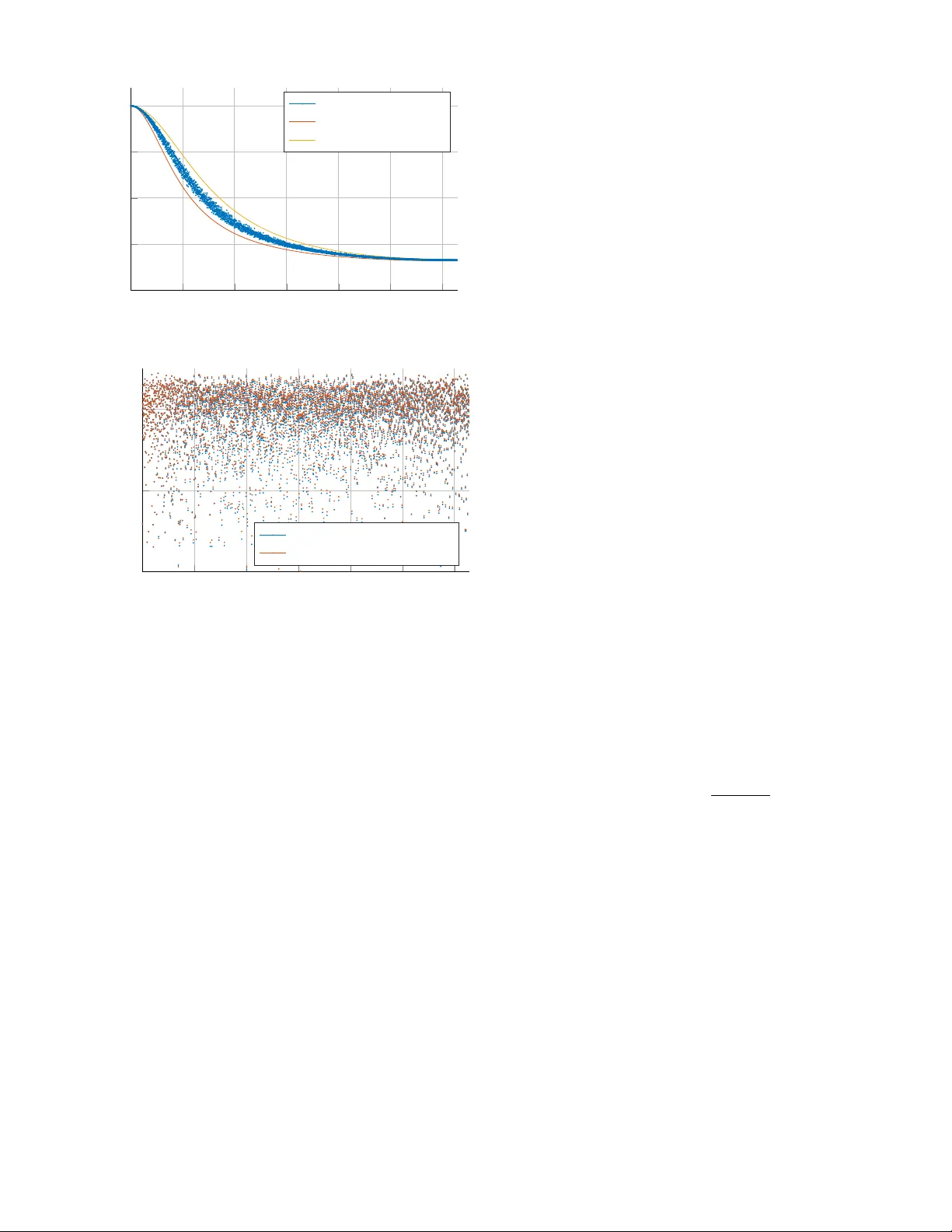
IEEE TRANSA CTIONS ON SIGNAL PR OCESSING, V OL. ?, NO. ?, ? 2018 1 Modal Decomposition of Feedback Delay Networks Sebastian J. Schlecht and Emanu ¨ el A. P . Habets, Senior Member , IEEE Abstract —Feedback delay networks (FDNs) belong to a general class of recursi ve filters which are widely used in sound synthesis and physical modeling applications. W e present a numerical technique to compute the modal decomposition of the FDN transfer function. The proposed pole finding algorithm is based on the Ehrlich-Aberth iteration for matrix polynomials and has impro ved computational performance of up to thr ee orders of magnitude compar ed to a scalar polynomial root finder . W e demonstrate how explicit knowledge of the FDN’ s modal behavior facilitates analysis and improvements for artificial r everberation. The statistical distribution of mode frequency and residue mag- nitudes demonstrate that relatively few modes contribute a large portion of impulse response energy . Index T erms —F eedback Delay Network, Modal Synthesis, Artificial Re verberation, Matrix Polynomial, Ehrlich-Aberth It- eration I . I N T R O D U C TI O N A feedback delay network (FDN) consists of a set of delay lines with lengths m which are interconnected via a feed- back matrix A (see Fig. 1). FDNs arise in many physical mod- eling applications where geometrically distributed components are approximated by time delays, e.g., strings [1], plates and membranes [2], springs [3], and air v olume [4, 5]. The interest in FDNs is fueled by the highly efficient implementation of delays in the time-domain, e.g., with circular buf fers resulting in a constant time complexity O (1) independent of its length. Therefore, the computational complexity of the FDN scales with the number of delay lines and not the system order . FDNs are a popular choice for artificial reverberation applications particularly because of the fav orable relation between FDN size and system order [6–9]. In this work, we present a modal decomposition technique for FDNs. The modal decomposition of a system is an equiv a- lent representation as the sum of complex one-pole resonators, so-called modes. The time-domain signal of such a resonator with pole λ i and residue ρ i is h i ( n ) = | ρ i || λ i | n e ı ( n ∠ λ i + ∠ ρ i ) , (1) where ∠ indicates the argument of a complex number in radiant, |·| is the magnitude, ı = √ − 1 and n indicates the discrete time index. Each indi vidual resonating mode is gov erned by four parameters: mode frequency ∠ λ i , decay rate | λ i | , initial phase ∠ ρ i and initial amplitude | ρ i | (see Fig 1). W ith modal decomposition, we aim to uncover the specific parameters of each mode. The time-domain impulse response of the FDN h ( n ) = N X i =1 h i ( n ) (2) is the sum of the complex modes h i ( n ) , where N is the system order . In sound synthesis applications for instance, the human A x b D m ( z ) c y F requency Decay Rate Amplitude Modal Decomposition Eq. (6) Modal Synthesis Eq. (1) Summation Eq. (2) Time-Domain Recursion Eq. (3) Time Amplitude Time Amplitude Fig. 1. Conceptual overvie w of modal decomposition and synthesis of a feedback delay network (FDN). T op left : FDN block diagram with a set of delay lines D m ( z ) , connected via a feedback matrix A , and input and output gains b and c for input and output signals x and y , respectiv ely . Thick lines indicate multiple signals. T op right : FDN modes with four parameters each: frequency , decay rate, initial amplitude and phase (not depicted). Bottom right : T ime-domain impulse responses of the resonators corresponding to the FDN modes. Bottom left : T ime-domain impulse response of the FDN. auditory system can recognize the spectral quality composed of the individual modes and this representation is therefore termed additive or modal synthesis [10]. Modal analysis of recursive systems is applied in various system modeling applications, ranging from acoustics and digital filter design to mechanical modeling [11]. A particularly challenging ap- plication for modal decomposition is room acoustics, where ev en medium room sizes e xhibits millions of modes [12]. Only for simple room geometries, an analytic expression for the system poles and residues can be stated [13]. System poles may also be recovered from the impulse response by various techniques such as an autoregressi ve moving-av erage [14], Bayesian inference [15] and all-pole modeling [16]. Whereas these techniques may be able to successfully compute partial solutions or compute the solution for specific configurations, the computation of the entire set of modes is in general challenging. In the following, we giv e the precise problem statement of this work. A. Pr oblem Statement For a single input and single output, the time-domain recursion of an FDN with N delay lines is gi ven by y ( n ) = c > s ( n ) + dx ( n ) s ( n + m ) = As ( n ) + b x ( n ) , (3) IEEE TRANSA CTIONS ON SIGNAL PROCESSING, V OL. ?, NO. ?, ? 2018 2 where n is the time index, · > denotes the transpose operation and A ∈ C N × N , b , c , s ( n ) ∈ C N × 1 , x ( n ) , y ( n ) , d ∈ C [17]. The state vector is defined as s ( n + m ) = [ s 1 ( n + m 1 ) , . . . , s N ( n + m N )] . W e write N -FDN to denote an FDN of size N . The transfer function of an FDN is H ( z ) = c >  D m ( z ) − 1 − A  − 1 b + d, (4) where D m ( z ) = diag( z − m 1 , z − m 2 , . . . , z − m N ) . The system order is giv en by N = P N i =1 m i [17]. For commonly used delays m , the system order is much larger than the FDN size, i.e., N  N . (5) The modal decomposition of the FDN, i.e., the partial fraction decomposition (PFD) of the transfer function (4) is H ( z ) = d + N X i =1 ρ i 1 − λ i z − 1 , (6) where ρ i is the residue of the pole λ i . The time-domain representation of the sum in (6) is giv en in (2) as the sum of complex resonators. The objecti ve of this work is to present an efficient numerical method to compute the modal decomposition (6) from the transfer function (4). B. Dir ect Appr oach W e first revie w two standard methods for the modal decom- position [17, 18]. Let A be any in v ertible matrix, then adj( A ) = det( A ) A − 1 , (7) where adj( A ) is the adjugate of the matrix A [19]. In the following, we denote P ( z ) = D m ( z ) − 1 − A . (8) W ith (7) and (8), the transfer function (4) can be expressed as a rational polynomial H ( z ) = q m , A , b , c ,d ( z ) p m , A ( z ) , (9) where p m , A ( z ) = det( P ( z )) (10) and q m , A , b , c ,d ( z ) = d det( P ( z )) + c > adj( P ( z )) b . (11) For brevity , we occasionally omit the parameters and write q ( z ) and p ( z ) . The FDN system poles λ i , where 1 ≤ i ≤ N , are the roots of the generalized characteristic polynomial (GCP) p m , A ( z ) in (10) such that they are fully characterized by the delay matrix D m ( z ) and the feedback matrix A . For a moment, let us assume that all delays are single time steps, i.e., m = 1 . The time-domain recursion in (3) reduces to the standard state-space description of a linear time- in v ariant (L TI) filter . The system poles λ i are the eigenv alues of the feedback matrix A such that the modal decomposition (6) is easily computed with standard methods. Ho wev er , for longer delays m such that (5) holds, the modal decomposition becomes more inv olv ed. The GCP p m , A can be expressed in a linearized fashion p m , A ( z ) = det( z I N − A ) , (12) where I N is the identity matrix of size N and A ∈ C N × N such that the system poles are the eigenv alues of A [17]. Unfortunately , for large delays m this eigen v alue problem becomes quickly numerically intractable. Alternatively , the GCP can be expressed as a scalar polynomial p m , A ( z ) = N X i =0 c i z i , (13) where the coefficients c i are deri ved from the principal minors of A [18]. The system poles are the roots of the scalar poly- nomial. Again, the polynomial degree increases with longer delays m and finding the roots of the polynomial becomes numerically intractable [20]. In the remainder of this paper, we present a numerically stable and computationally efficient method to compute the modal decomposition for large system order N and modest- sized N . In Section II, we deriv e the fundamental algorithm based on a polynomial matrix formulation. In Section III, we ev aluate the performance of the proposed algorithm. In Sec- tion IV, we apply modal decomposition to analyze the ef fects of attenuation filters and to study the statistical distributions of mode frequencies and residue magnitudes. I I . N U M E R I C A L M O D A L D E C O M P O S I T I O N In the following, we present a root finding algorithm for the GCP p ( z ) and subsequently recover the residues ρ i . W e conclude this section with a generalization to additional filtering in the delay lines and feedback matrix. A. P olynomial Matrix F ormulation It is a common heuristic in numerical computation that the inherent problem structure shall be preserved as much as possible throughout all computation steps to improv e numer- ical performance. In contrast to Section I-B, we compute the system poles without expanding the problem. In fact, (10) is a polynomial eigenv alue problem of degree K = max m , i.e., P ( z ) = K X k =0 P k z k , (14) where P k ∈ C N × N for 0 ≤ k ≤ K . For a proper matrix polynomial P ( z ) , i.e., det( P K ) 6 = 0 , the number of roots is K N [21]. For FDNs, howe ver , P K is singular such that the actual number of roots is lower , respectiv ely , man y roots are infinite. In fact, if det( A ) 6 = 0 , the number of finite roots is N which is also the degree of the scalar polynomial in (10) [18]. In the following, we use the deriv ati ve of the polynomial p ( z ) = det( P ( z )) . According to Jacobi’ s formula [22], we hav e p 0 ( z ) = d d z p ( z ) = det( P ( z )) tr  P ( z ) − 1 P 0 ( z )  = tr(adj( P ( z )) P 0 ( z )) , (15) IEEE TRANSA CTIONS ON SIGNAL PROCESSING, V OL. ?, NO. ?, ? 2018 3 where P 0 ( z ) = d P ( z ) d z and tr( X ) denotes the trace of matrix X . Ste wart [23] showed that the adjugate of A can be well- conditioned e ven when A is ill-conditioned, and he sho ws ho w adj( A ) can be computed in a numerically stable way from a rank rev ealing decomposition of A [22]. With the definitions of the polynomial eigen v alue problem introduced, we present the proposed root finding algorithm. B. Ehrlich-Aberth Method The polynomial eigenv alue problem can be solved with the Ehrlich-Aberth Iteration (EAI) method, i.e., a combination of Newton method and a deflation term which prevents that two eigen v alues conv erge to the same solution [21]. Let λ (0) ∈ C N be a vector of initial estimates for the N roots of the polynomial p ( z ) and λ ( j ) = [ λ ( j ) 1 , λ ( j ) 2 , . . . , λ ( j ) N ] be the j -th EAI iteration. The EAI pro vides the sequence of estimates λ ( j +1) i = λ ( j ) i − ∆ ( j ) i (16) with the EAI step being ∆ ( j ) i = N  λ ( j ) i  1 − N  λ ( j ) i  D i  λ ( j )  . (17) Using the identity in (15), the Newton correction term is N ( z ) = p ( z ) p 0 ( z ) = 1 tr( P ( z ) − 1 P 0 ( z )) (18) and the deflation term is D i  λ ( j )  = N X l =1 ,l 6 = i 1 λ ( j ) i − λ ( j ) l . (19) The deflation term may be interpreted as a penality term if two eigen v alues approach each other too closely and guarantees that the all eigenv alues reached are unique. Using (18) we can expand (17) to ∆ ( j ) i = 1 tr  P  λ ( j ) i  − 1 P 0  λ ( j ) i   − D i  λ ( j )  . (20) The method, giv en here in the Jacobi version, is known to con v erge cubically for simple roots and linearly for multiple roots [21]. The Gauss-Seidel v ersion of EAI [21], which updates the estimates as soon as they become av ailable, may con v erge even slightly f aster . C. Stopping Criteria The system poles λ i are the roots of the polynomial p ( z ) in (10), i.e., det( P ( λ i )) = 0 . In other words, P ( λ i ) is a singular matrix for all system poles. Thus, the natural stopping criteria is the reciprocal of the condition number κ ( P ( z )) being less than a prescribed tolerance τ 1 . This stopping condition is also computationally fa vorable as the condition number can be estimated highly efficiently [22]. Howe ver , for multiple eigen v alues this stopping condition may result in a premature halt [21]. An alternativ e stopping condition says that the computed correction is too tiny and would not change the significant digits of the current estimate    ∆ ( j ) i    ≤ τ 2    λ ( j ) i    , (21) where τ 2 is a small positiv e tolerance threshold [21]. In practice, good global con v ergence properties are observed; a theoretical analysis of global conv er gence, though, is still missing and constitutes an open problem. There is empirical evidence that the number of Ne wton iterations heavily depends on the choice of the initial estimates [21]. D. Initialization Aberth [24] proposed to choose initial estimates placed along a circle centered at the origin of sufficiently large radius so that it contains all the roots. In case the magnitude of the roots vary largely , multiple circles with suitable radii may be chosen instead [25]. W ith Rouch ´ e’ s theorem, we can deriv e upper and lower bounds on the pole magnitudes for the FDN depending on the singular values σ ( A ) of the feedback matrix (see Appendix A) min m p min σ ( A ) ≤ | λ i | ≤ max m p max σ ( A ) . (22) Equation (22) is a generalization on the relation of eigen values and singular v alues as gi ven in the W eyl-Horn Theorem [26] in the case of unit delays m = 1 . The bound is tight for a diagonal feedback matrix where the minimum and maximum delays coincide with the minimum and maximum diagonal element, respecti vely . Howe ver , the bound may be arbitrarily loose. F or instance, the maximum singular v alue of a triangular matrix max σ ( A ) may be arbitrarily large while all system poles lie on the unit circle [9]. F or lar ge delays m howe ver , (22) shows that the pole magnitudes tend to be close to the unit circle. W e can further deriv e from (22) that if max σ ( A ) ≤ 1 then all poles lie on the closed unit disk which is equiv alent to the FDN being marginally stable [27]. In particular, if all singular values are 1, which is equiv alent to A being unitary , i.e., A H A = I , all system poles lie on the unit circle regardless of the delays m . Such an FDN is called lossless, and represents an important special case [9]. In this work, we are interested in lossless and stable FDNs for their practical relev ance. In combination with (5), such FDNs have all poles in the unit disk, but close to the unit circle. Thus, we place the initial estimates λ (0) uniformly on the unit circle. More precisely , we chose the roots of unity λ (0) = exp  ı 2 π  0 N , 1 N , . . . , N − 1 N  . (23) It is worthwhile to note that λ (0) is the solution of a particular FDN with a circular shift matrix A = I S =        0 1 0 · · · · · · 0 0 0 1 · · · · · · 0 . . . . . . . . . . . . 1 0 0 0 0 · · · 0 1 1 0 0 · · · 0 0        (24) IEEE TRANSA CTIONS ON SIGNAL PROCESSING, V OL. ?, NO. ?, ? 2018 4 such that the GCP is p m , I S ( z ) = z N − 1 . (25) The shift matrix thus combines the FDN delays into a single long delay line. E. Appr oximate Deflation For a high system order N , the computational complexity of the deflation term (19) may become excessi v e. W e propose an appr oximate deflation (AD) according to a maximum error tolerance τ 3 for the resulting EAI step e ∆ ( j ) i in (20), i.e.,    ∆ ( j ) i − e ∆ ( j ) i    ≤ τ 3 . (26) The magnitude of the deflation term summands decreases with the pole distance λ ( j ) i − λ ( j ) l . The idea is then to divide the poles into a near and far pole sets, λ ( j ) near and λ ( j ) far , respecti vely , and approximate the deflation of the less significant far poles λ ( j ) far by a default term, e.g., λ (0) far . For symmetry , the number of near poles N near is assumed to be an e ven number . It can be shown, that for equidistributed poles such as λ (0) in (23), the far deflation is (see Appendix B) D i  λ (0) far  = 1 λ (0) i N − N near − 1 2 . (27) Thus, the total deflation may be approximated by f D i  λ ( j )  = D i  λ ( j ) near  + D i  λ (0) far  (28) if the far poles λ ( j ) far are suf ficiently uniformly distributed. By sorting the system poles iterations along pole angles, we can find the near poles λ ( j ) near . T o establish the quality of this approximation, let us assume that there exists an upper bound  D for the approximation error of the deflation term, i.e.,  D ≥ max i,j    f D i  λ ( j )  − D i  λ ( j )     . (29) W e can show that the error tolerance τ 3 in (26) is satisfied if (see Appendix C)     N  λ ( j ) i  − 1 − f D i  λ ( j )      −  D ≥ 2 τ 3 . (30) In other words, if the deflation approximation is sufficiently far from the in verse Newton term, the deflation error becomes negligible. On the contrary , if the deflation term is close to the in v erse Newton step, the EAI step error can be large ev en for small deviations in the deflation term. In case the error tolerance in (30) is not satisfied, we compute the e xact deflation instead. T o implement the proposed approximate deflation, we need a priori knowledge of the approximation error bound  D . As  D depends on many factors such as matrix size N , system order N , feedback matrix A and number of near poles N near , in this work, it is determined experimentally from random FDNs. The performance of the approximate deflation method may be quantified by the number of exact deflations versus approximate deflations. As the initial estimates λ (0) are equidistributed, λ (1) may be computed only from the estimated far deflation with N near = 0 . F . Residues Once we hav e found the system poles, the residues of the modal decomposition (6) are computed by ρ i = q ( λ i ) p 0 ( λ i ) , (31) where we assume that all poles are unique. Similar , but more intricate solutions exists for non-unique poles [28]. The undriv en residue, i.e., the system response without excitation, is ρ u i = 1 p 0 ( λ i ) . (32) The undriv en residue is a v aluable intermediate step to analyze the mode initial amplitude independent from the input and output driv es q ( λ i ) . Since, P ( λ i ) is a singular matrix, the deriv ative of the GCP p 0 ( λ i ) in (15) may only be computed by the adjugate formulation. Since det( P ( λ i )) = 0 , the input- output driv es in (11) are q ( λ i ) = c > adj( P ( λ i )) b . (33) The difference between the driven and undri ven residues may be expressed as a linear combination of the matrix entries of adj( P ( λ i )) . Alternatively , the driv en residues may also be computed by a least linear squares fit for the time-domain impulse response since the sum of complex resonators in (2) depends linearly on the residues [29]. G. P olynomial F eedbac k and Delay Matrices Although, the focus of this work is on frequency- independent feedback matrices A , much of the dev elopment in Section II is applicable to general polynomial matrices. Therefore, it is easy to include further filtering such as a frequency-dependent feedback matrix A ( z ) . There also exists a singular value decomposition for polynomial matrices A ( z ) [30]. Alternatively , the delay lines are often extended with an attenuation or allpass filter α i ( z ) , i.e., D m ( z ) α ( z ) = diag  z − m 1 α 1 ( z ) , . . . , z − m N α N ( z )  . (34) It is important to note that additional filters may increase the number of system poles. Further, if P ( z ) is a rational polynomial, in other words consists of IIR filters, then the transfer function in (4) is no longer proper, i.e., the polynomial degree of the nominator is larger than the polynomial degree of the denominator [31]. Nonetheless, improper partial fraction decomposition can be solved with a delayed parallel form by separating the FIR and IIR part of the transfer function [29]. For a unitary feedback matrix A and for attenuation filters in (34), it is possible to improve the pole magnitude bounds (22) to min  α  e ı ∠ λ i  1 / m  ≤ | λ i | ≤ max  α  e ı ∠ λ i  1 / m  , (35) where all v ector operations are element-wise (see Ap- pendix A). I I I . M O D A L S Y N T H E S I S A N D E V A L UA T I O N The following ev aluation uses real-valued FDN parameters such that the system poles appear in complex conjugate pairs. IEEE TRANSA CTIONS ON SIGNAL PROCESSING, V OL. ?, NO. ?, ? 2018 5 5 10 15 20 25 30 2 3 4 5 6 Matrix Size N A verage Number of Iterations det ( A ) = +1 det ( A ) = − 1 Fig. 2. A v erage number of full iterations in the EAI for 500 random FDNs with total delay N between 50 and 10 4 samples and a random orthogonal feedback matrix. The average number of full iterations indicate the av erage number of Newton steps each pole requires to con verge. For low matrix size N , the sign of matrix determinant det( A ) and parity of N plays a significant role. A. Modal Synthesis and Accuracy A numerically accurate way to verify the modal decompo- sition is to synthesize each mode h i ( n ) in time-domain as expressed in (1) and compare the sum of all modes with the impulse response h ( n ) computed by the time-domain recur- sion in (3). The concept of modal synthesis and verification is depicted in Fig. 1. The error is giv en by the maximum difference 1 between the two impulse responses, i.e.,  = max n      h ( n ) − N X i =1 h i ( n )      . (36) In this work, we use double precision floating point arithmetic and the modal decomposition is regarded successful if the maximum error  < 10 − 10 . The EAI is numerically stable as the matrix in v ersion in (20) is only necessary if the matrix is sufficiently non-singular due to the first stopping criteria. For large delays m , the ev aluation of D m ( z ) may become extremely large or small if z is too far away from the unit circle. At the same time, the poles tend to be close to the unit circle for large delays m due to the bounds given in (22). As a practical intervention, the pole location is clipped to the magnitude bounds if the EAI step causes the pole location to exceed the bounds. B. Numerical Evaluation For the FDN, a single EAI step in (20) can be ev aluated in O ( N + N 3 ) : an ev aluation of P ( z ) and P 0 ( z ) is merely an ev aluation of the delay matrix D m ( z ) in O ( N ) ; a numer- ical matrix in version can be performed in O ( N 3 ) ; and the deflation term is ev aluated in O ( N ) . Thus, a full iteration from λ ( j ) → λ ( j +1) can be e valuated in O ( N 2 + N N 3 ) . 1 The maximum error is chosen as it is an upper bound for the root mean squared error (RMSE) and as such a strict error measure. 10 2 10 3 10 4 10 5 10 6 10 − 2 10 − 1 10 0 10 1 10 2 10 3 10 4 System Order T ime [s] EAI EAI AD eig roots Fig. 3. Computation time comparison of EAI with MA TLAB build-in func- tions eig and roots . For system order N > 5 · 10 4 , the memory requirements of eig and roots become prohibitive on a personal computer configuration. The results are identical to a maximum error less than  < 10 − 10 . This compares fa v orably with the bound O ( N 3 ) of a matrix- based algorithm applied to the linearization in (12). For a high number of system poles N  N 3 , the complexity of computing the deflation term in (19) becomes the dominating part. The complexity of the approximate deflation in (28) is similar asymptotically , howe v er in practice, the computational complexity is reduced significantly . Fig. 2 sho ws the average number of full iterations depending on the matrix size N , total delays N between 50 and 10 4 samples and a random orthogonal feedback matrix. It can be seen that the number of iterations is largely dependent on the parity of the matrix size and det( A ) . This illustrates how the initialization (23) influences the performance of the EAI. Overall, about 4 to 5 iterations per root may be expected for the EAI to conv erge. Fig. 3 depcits a comparison of measured computation time with the MA TLAB 2 functions eig and r oots solving the direct problems (12) and (13), respectiv ely . The total number of delays N were distributed randomly among eight delay lines and the feedback matrix A ∈ R 8 × 8 was a random orthogonal matrix. All methods gav e the correct answer with the required accuracy . For the approximate deflation, the number of near poles N near was set to N / 100 . The maximum deflation error  D = 10 3 was determined a priori by probing an independent set of random FDNs of similar configuration. The EAI step tolerance τ 3 was set to 10 − 3 . The EAI implementation utilizes only standard MA TLAB functions and no C-optimization which e xplains relati vely poor performance for small system order N < 10 3 . For high system order N such as 5 · 10 4 , the standard EAI and EAI with AD outperform the MA TLAB’ s eig function by a factor of more than 300 and 1300, respectiv ely . Further , the memory requirements of the EAI are only linear in N and cubic in N such that it is possible to perform modal decomposition up to N = 10 6 . Whereas the memory requirements for eig become 2 Matlab is a registered trademark of The MathW orks Inc. All computations were performed with Matlab R2016b on a desktop machine with an Intel Core i7 @ 3,40 GHz and 32 GB of RAM. IEEE TRANSA CTIONS ON SIGNAL PROCESSING, V OL. ?, NO. ?, ? 2018 6 0 0 . 5 1 1 . 5 2 2 . 5 3 0 0 . 5 1 1 . 5 2 Pole Angular Frequency [rad] Pole R T60 [s] Poles with attenuation Minimum Bound Maximum Bound (a) System pole magnitudes 0 0 . 5 1 1 . 5 2 2 . 5 3 − 120 − 100 − 80 Pole Angular Frequency [rad] Residue Magnitude [dB] Residues with attenuation Residues without attenuation (b) System residue magnitudes Fig. 4. Modal Decomposition of 8-FDN with target rev erberation time T 60 (0) = 2 seconds and T 60 ( π ) = 0 . 4 seconds using one-pole attenuation filters [7]. Delays are m = [2300 , 499 , 1255 , 866 , 729 , 964 , 1363 , 1491] and A is a random orthogonal matrix. (a) Pole magnitudes con verted to rev erberation time. Minimum and maximum bounds are computed from (35). (b) Residue magnitudes with and without attenuation. The mean difference between the residue magnitudes is 0.48 dB. prohibitiv e for N > 5 · 10 4 . For N > 10 5 , more the 95% of the computation time of the standard EAI was spent on the deflation term. For the EAI with AD, the number of exact iterations nev er exceeded 1% of the total number of iterations proofing the chosen heuristic parameters effecti ve. The EAI with AD performs similar for small delays but outperforms the standard EAI by a factor of 100 for large delays. Each EAI step is independent and only requires synchronization at ev ery full iteration step such that the overall performance of the EAI might further be improv ed by parallelization. I V . A N A L Y S I S O F F E E D B AC K D E L AY N E T W O R K S W e study two applications of modal decomposition in arti- ficial rev erberation: Firstly , we study the effect of attenuation filters on the poles and residues of an FDN. Secondly , we study the statistical distribution of poles and residues of random lossless FDNs. A. Attenutation Attenuation filters in FDNs, as they are typically applied in artificial rev erberation, aim to control the frequency-dependent rev erberation time [7, 32]. As expressed in (34), all delays are extended with absorption filters α ( z ) and the feedback matrix A is orthogonal or more generally unilossless [9]. W e study three types of attenuation: homogeneous, near-homogeneous and inhomogeneous attenuation. 1) Homogeneous Attenuation: The attenuation filters α ( z ) are called homogeneous if there e xists an attenuation-per - sample Γ( z ) such that α i ( z ) = Γ( z ) m i . (37) The attenuated delay lines can be expressed as plain delay lines with a mapped ar gument, i.e., D m ( z ) α ( z ) = D m ( z Γ( z ) − 1 ) . (38) Consequently , the system poles with attenuation λ Γ i can be related to the system poles λ i without attenuation by λ i = λ Γ i Γ( λ Γ i ) − 1 . (39) If we assume that the attenuation filters hav e a purely real frequency response 3 , i.e., Γ( e ıω ) ∈ R then the mode frequen- cies are unaltered by the attenuation, i.e., ∠ λ i = ∠ λ Γ i . F or a unilossless A , all unattenuated system poles λ i lie on the unit circle such that   λ Γ i   = Γ( λ i ) (40) and the attenuated FDN is stable if | Γ( e ıω ) | < 1 . For homogeneous attenuation, the magnitude bounds in (35) are tight. 2) Near-homo geneous Attenuation: T ypically , the attenua- tion filters are implemented with relatively low order , such as one-pole filters [7], ho we ver higher order filters were proposed as well [32, 33]. The attenuation filters are designed to match the magnitude response | α i ( e ıω ) | ≈ | Γ( e ıω ) m i | , (41) where the attenuation-per-sample is deriv ed from a target rev erberation time 20 log 10 | Γ( e ıω ) | = − 60 T 60 ( ω ) f s , (42) where f s is the sampling frequency and T 60 ( ω ) is the time in seconds for the energy decay curve of the impulse response at frequency ω to decay by 60 dB [34]. F or illustration, we compute the one-pole filter according to [7] giv en the target rev erberation time at DC T 60 (0) and Nyquist frequency T 60 ( π ) . Figure 4 depicts the resulting modal decomposition for an 8-FDN with an orthogonal feedback matrix and a target rev erberation time T 60 (0) = 2 seconds and T 60 ( π ) = 0 . 4 sec- onds. The system pole magnitudes are modified according to the target re verberation time. Howe ver , the attenuation varies especially in the transition band due to errors in the magnitude response caused by the limited filter order . The magnitude of the residues are depicted in Fig. 4b. For near-homogeneous attenuation, it can be observed that the residues with and without attenuation are rather similar . Although the attenuation filters are not completely homogeneous, their phase component 3 Although such a frequency response is not realizable with a digital filter in general, b ut useful for the theoretical analysis. IEEE TRANSA CTIONS ON SIGNAL PROCESSING, V OL. ?, NO. ?, ? 2018 7 0 0 . 5 1 1 . 5 2 2 . 5 3 0 1 2 3 Pole Angular Frequency [rad] Pole R T60 [s] Poles with attenuation Minimum bound Maximum bound Fig. 5. Modal Decomposition of 8-FDN with inhomogeneous attenuation α ( z ) according to an average delay length m = 1074 for all one- pole attenuation filters in (41). Identical delays, feedback matrix and target rev erberation time as in Fig. 4 were used. Minimum and maximum bounds are computed from (35). is small compared to the phase of the delays z − m such that the ov erall beha vior is well approximated by (40). This suggests that studies on residues of lossless systems may translate well to results for moderately lossy systems. 3) Inhomogeneous Attenuation: While the homogeneous attenuation has perceptually desirable properties in artificial rev erberation, more physically oriented FDN designs such as scattering delay networks [35] and radiance transfer [36] employ attenuation filters which are unrelated to the delay lengths but related to the boundary materials of the simulated space. Figure 5 depicts the modal decay rate of the same 8- FDN as in Fig. 4 with different attenuation filters. Instead of the delay proportional design in (41), all one-pole filters hav e the same target frequency response corresponding to an av erage delay length. As a consequence, the decay time of the neighboring modes are largely different, while the ov erall shape still follows the target re verberation time. B. Statistical Distribution of P oles and Residues W e present a set of statistical analyses of lossless FDNs which rely on the proposed large-scale numerical computation of the modal decomposition and are difficult to deriv e by analytic methods. The statistical analysis answers a long- standing question in artificial re verberation design [37]: Why do some FDNs have an unpleasant metallic ringing despite a sufficiently high modal density ? While ideal late re verberation has been characterized as Gaussian white noise [38], the metal- lic ringing is caused by excessi v e energy at few frequencies. In terms of modal decomposition, metallic ringing may be caused by either clustering of multiple poles at the ringing frequencies or largely varying energy of neighboring modes. W e study the following two questions: 1) What is the distribution of the mode frequencies? 2) What is the distribution of residue magnitudes? In the analyses, we rely on Monte Carlo simulations of randomly generated lossless FDNs. 1) Mode F r equency Distribution: The near-equidistribution of mode frequencies has been conjectured before [39] and the T ABLE I P RO BA B I LI T Y C H IS T ( κ ) O F C L US T E R N UM B E RS O F M O DE F R E QU E N CI E S Cluster size κ 0 1 2 3 ≥ 4 Uniform Random 0.3690 0.3661 0.1854 0.0610 0.0186 Lossless 8-FDN 0.1694 0.6632 0.1653 0.0020 0.0001 Equidistributed 0.0000 1.0000 0.0000 0.0000 0.0000 authors hav e giv en an analytical bound on the equidistribution based on Hayman’ s theorem [18]. The cluster number C ( ω ) = # n i    ∠ λ i ∈ h ω − π N , ω + π N io , (43) is a measure on how equally distributed the mode frequencies are. Here, # denotes the cardinality of a set. The higher the cluster number , the more poles cluster around the frequency ω . In contrast, a mode gap occurs if C ( ω ) = 0 , i.e., no mode lies in this frequency interv al. F or perfectly equidistributed poles C ( ω ) = 1 for all ω . W e ev aluate the distribution of mode frequencies by computing the histogram of cluster numbers C HIST ( κ ) = L X l =1 δ  C  2 π l L  − κ  , (44) where δ ( · ) is the dirac function, κ is the integer cluster size, and L is the number of observations. For large enough L , the histogram conv erges tow ards the probability of cluster num- bers. The random 8-FDNs hav e delays between 50 and 1000 samples and an orthogonal feedback matrix. The probabilities are av eraged over 100 random instances each. In T able I, the probability of cluster numbers for randomly generated FDNs are compared to cluster numbers of a pseudo- uniform random number generator with equal sampling size. The discrepanc y of the cluster number from an equidistribution is relatively low for the FDN modes compared to the random number generator . In fact for FDNs, it is very rare to find an interval of width 2 π / N with more than two modes. In stark contrast, acoustic mode density of physical spaces increase quadratically with frequency [12]. 2) Residue Magnitude Distribution: In Section II-F, we hav e presented the computation of the mode residues for a giv en set of system poles. Figure 6 depicts the magnitude histogram of the total and undri ven residues as well as the input-output driv es for a random 8-FDN. The input-output driv es are comprised of all individual input-output combina- tions, i.e., adj( P ( λ i )) in (33). The total residues ρ ( λ i ) result from unit input and output gains, i.e., b = 1 and c = 1 , or in other words, ρ ( λ i ) = ρ u ( λ i )( 1 > adj( P ( λ i )) 1 ) . The magnitude distributions of the in verse undriven residues 1 /ρ u ( λ i ) , the total residues ρ ( λ i ) and input-output drives adj( P ( λ i )) all resemble log-Rayleigh distributions [40]. Howe v er , just by altering the feedback matrix A , it is possible to encounter various other distributions of the residue magnitude. Figure 7, depicts the residue magnitude distribution of four selected orthogonal feedback matrices. 3) Discussion: For randomly generated FDNs, the mode frequencies are nearly equidistributed such that ev ery fre- quency band has ener gy contributions from a similar number IEEE TRANSA CTIONS ON SIGNAL PROCESSING, V OL. ?, NO. ?, ? 2018 8 − 100 − 80 − 60 − 40 − 20 0 20 0 200 400 Residue Magnitude [dB] Number of Residues Input-Output Dri v es T otal Residue Undriv en Residue Fig. 6. Histogram of residue magnitude of an 8-FDN with delays m = [492 , 794 , 1849 , 1855 , 1155 , 1090 , 78 , 1957] and a random orthogonal feed- back matrix A . The undriven residues ρ u ( λ i ) are dependent only on the feedback loop P ( z ) , whereas the total residues ρ ( λ i ) results from unit input and output gains, i.e., b = 1 and c = 1 , respecti vely . The input-output drives q ( λ i ) are the 8 × 8 magnitudes of the adjugate matrix adj( P ( λ i )) . of modes. On the other hand, the high dynamic range of the residue magnitudes suggest that a small number of poles contribute a large portion of the impulse response energy . In the context of artificial re v erberation, the high-energy modes dominate the frequency spectrum such that the audible modal density is considerably lower than theoretic modal density , i.e., the number of modes per frequency . For illustration, we have synthesized audio examples from the four instances depcited in Fig. 7 and pro vided them online 4 . The residue distribution may be optimized in two steps: Firstly , optimization of the undriv en residues by choosing delays m and feedback matrix A . Secondly , optimization of the total residue by choosing the input and output gains, b and c . While the first step is a non-linear process which requires further research, the second step may be readily solved by linear least square fitting. V . C O N C L U S I O N W e presented a numerically efficient technique for modal decomposition of the FDN. Standard methods such as eigen- value decomposition of the linearized system and polynomial root finding methods applied to the characteristic polynomial require significant computational resources when the system order is large. The proposed method applies the Ehrlich- Aberth Iteration to the polynomial matrix formulation of the FDN. Further we proposed, an efficient approximate deflation technique based on the estimation of far poles. F or high system order such as 5 · 10 4 , the standard EAI and approximate EAI outperform the MA TLAB’ s eig function by a factor of more than 300 and 1300, respectiv ely . The approximate EAI was able to giv e reliable results up to a system order of 1 million. The modal decomposition was applied to FDNs in the context of artificial rev erberation. Three types of at- tenuation were studied: homogeneous, near-homogeneous and 4 www .audiolabs- erlangen.de/resources/2018- IEEE- Modal − 120 − 110 − 100 − 90 − 80 − 70 − 60 0 200 400 600 800 Residue Magnitude [dB] Number of Residues A 1 A 2 A 3 A 4 Fig. 7. Histograms of the residue magnitude with delays m = [492 , 794 , 1849 , 1855 , 1155 , 1090 , 78 , 1957] for four different orthogonal matrices A 1 , A 2 , A 3 and A 4 . The four matrices are chosen manually from 1000 random orthogonal matrices to display a variety of residues magnitude distributions. inhomogeneous. The potential for explicit analysis of the pole and residues was demonstrated for attenuation filter design. Statistical analysis sho wed that for randomly generated FDNs, the mode frequencies are nearly equidistrib uted and the residue magnitudes follow a log-Rayleigh distribution. This analysis suggests that relatively few modes are contrib uting a large portion of the late re verberation energy . A P P E N D I X A L OW E R B O U N D O F P O L E M A G N I T U D E W e present lo wer and upper bounds on the pole magnitudes | λ | of an FDN. The bounds are based on the generalization of Rouch ´ e’ s theorem to matrix polynomials. Theorem 1 (see [41]) . Let S ( z ) and Q ( z ) be matrix polyno- mials and let r be a positive real number . If S ( z ) H S ( z ) − Q ( z ) H Q ( z ) is positive definite for | z | = r , then the polynomi- als det( S ( z )) and det( S ( z ) + Q ( z )) have the same number of r oots of modulus less than r . An immediate consequence of the abov e theorem applied to the polynomial P ( z ) of (8) with S ( z ) = − A and Q ( z ) = D m ( z ) − 1 is [21]: If A H A − D m ( z ∗ ) − 1 D m ( z ) − 1  0 , for | z | = r (45) where X  Y means that X − Y is positiv e definite, then P ( z ) has no eigen values in the open disk with center 0 and radius r . The criterium in (45) is equiv alent to A H A  D m ( r − 2 ) (46) which in turn is equi v alent to [42] ρ  ( A H A ) − 1 D m ( r − 2 )  ≤ 1 , (47) IEEE TRANSA CTIONS ON SIGNAL PROCESSING, V OL. ?, NO. ?, ? 2018 9 where ρ ( X ) denotes the spectral radius of a matrix X . Using properties of the spectral norm [42] we can giv e an upper bound on this expression by ρ  ( A H A ) − 1 D m ( r − 2 )  ≤    ( A H A ) − 1 D m ( r − 2 )    2 ≤   A − 1   2   A − H   2   D m ( r − 2 )   2 =   A − 1   2 2   D m ( r − 2 )   2 . (48) Thus, the criterium (47) is satisfied if r 2 min m =   D m ( r − 2 )   2 ≤   A − 1   − 2 2 = min σ ( A ) 2 . (49) Therefore with (45), the pole magnitude lower bound may be giv en as min | λ | ≥ min σ ( A ) 1 / min m . (50) Analogously , applying the same arguments to the re versed matrix polynomial z max m P ( z − 1 ) yields an upper bound max | λ | ≤ max σ ( A ) 1 / max m . (51) For additional attenuation filters α ( z ) as in (34) and a unitary feedback matrix A , these bounds can be tightened further . Rouch ´ e’ s criterion (45) gi ves the relation α ( z )  | z | m . (52) Thus, the lower bound of the pole magnitude is | λ i | ≥ min  α  e ı ∠ λ i  1 / m  . (53) The corresponding upper bound may be derived similar to (51): | λ i | ≤ max  α  e ı ∠ λ i  1 / m  . (54) These bounds are tight for a diagonal matrix A . A P P E N D I X B F A R D E FL A T I O N E S T I M A T I O N W e are gi ven the equidistributed poles λ (0) as defined in (23) and an ev en number of near poles N near . W e compute the far deflation for pole λ ( j ) i . First we state a useful identity . For any real x , 1 1 − e ıx + 1 1 − e − ıx = 1 . (55) The total deflation is D i  λ (0)  = N X l =1 ,l 6 = j 1 λ (0) i − λ (0) l = 1 λ (0) i N X l =1 ,l 6 = j 1 1 − λ (0) l /λ (0) i = 1 λ (0) i N X l =1 ,l 6 = j 1 1 − exp  ı 2 π l − j N  = 1 λ (0) i N − 1 2 . Similarly , as each conjugate pair of poles contribute equally to the deflation, the far deflation is D i  λ (0) far  = 1 λ (0) i N − N near − 1 2 . (56) A P P E N D I X C D E FL A T I O N E R RO R W e sho w that inequality (30) is sufficient for inequality (26). For the sake of bre vity , we omit the pole arguments in the following. Given the deflation approximation f D i , which satisfy (30), we obtain τ 3 2 ≥ 1    N − 1 − f D i    −  D ≥ 0 . (57) W e show that (57) satisfies EAI step error tolerance (26). Because  D ≥ 0 , it is τ 3 2 ≥ 1    N − 1 − f D i    ≥ 0 . (58) Further , as    D i − f D i    −  D ≤ 0 , 1 |N − 1 − D i | ≤ 1 |N − 1 − D i | +    D i − f D i    −  D ≤ 1    N − 1 − f D i    −  D ≤ τ 3 2 Eventually , we can show that    ∆ ( j ) i − e ∆ ( j ) i    ≤     1 N − 1 − D i − 1 N − 1 − f D i     ≤     1 N − 1 − D i     +     1 N − 1 − f D i     ≤ τ 3 R E F E R E N C E S [1] K. Karplus and A. Strong, “Digital synthesis of plucked- string and drum timbres, ” Comput. Music J . , vol. 7, no. 2, pp. 43–55, 1983. [2] J. O. Smith III, “Physical modeling using digital wa ve g- uides, ” Comput. Music J. , v ol. 16, no. 4, pp. 74–91, 1992. [3] J. D. Parker , “Efficient dispersion generation structures for spring reverb emulation, ” EURASIP J. Adv . Signal Pr ocess. , vol. 2011, no. 1, pp. 1–8, 2011. [4] L. Savioja and U. P . Svensson, “Overvie w of geometrical room acoustic modeling techniques, ” J . Acoust. Soc. Amer . , vol. 138, no. 2, pp. 708–730, Aug. 2015. [5] V . V ¨ alim ¨ aki, J. D. Parker , L. Savioja, J. O. Smith III, and J. S. Abel, “Fifty years of artificial rev erberation, ” IEEE/A CM T rans. Audio, Speech, Lang. Proc. , vol. 20, no. 5, pp. 1421–1448, Jul. 2012. [6] M. A. Gerzon, “Synthetic stereo re verberation: Part One, ” Studio Sound , vol. 13, pp. 632–635, 1971. [7] J. M. Jot and A. Chaigne, “Digital delay networks for designing artificial re verberators, ” in Pr oc. Audio Eng. Soc. Con v . , Paris, France, Feb . 1991, pp. 1–12. [8] S. J. Schlecht and E. A. P . Habets, “Feedback delay networks: Echo density and mixing time, ” IEEE/ACM T rans. Audio, Speech, Lang. Pr oc. , vol. 25, no. 2, pp. 374–383, 2017. [9] ——, “On lossless feedback delay networks, ” IEEE T rans. Signal Pr ocess. , vol. 65, no. 6, pp. 1554–1564, Mar . 2017. IEEE TRANSA CTIONS ON SIGNAL PROCESSING, V OL. ?, NO. ?, ? 2018 10 [10] J.-M. Adrien, “The missing link: modal synthesis. ” MIT Press, May 1991, pp. 269–298. [11] J. He and Z.-F . Fu, Modal Analysis . Oxford, UK: Butterworth-Heinemann, 2001. [12] H. Kuttruff, Room Acoustics, F ifth Edition . CRC Press, Jun. 2009. [13] Y . Naka, A. A. Oberai, and B. G. Shinn-Cunningham, “ Acoustic eigen values of rectangular rooms with arbitrary wall impedances using the interv al Newton / generalized bisection method, ” J. Acoust. Soc. Amer . , vol. 118, no. 6, pp. 3662–3671, Dec. 2005. [14] M. Karjalainen, P . A. A. Esquef, P . Antsalo, A. Maki virta, and V . V ¨ alim ¨ aki, “AR/ARMA analysis and modeling of modes in resonant and rev erberant systems, ” in Pr oc. Audio Eng. Soc. Conv . , Munich, Germany , May 2002, pp. 1–16. [15] D. Beaton and N. Xiang, “Room acoustic modal analysis using Bayesian inference, ” J. Acoust. Soc. Amer . , vol. 141, no. 6, pp. 4480–4493, Jun. 2017. [16] Y . Haneda, S. Makino, and Y . Kaneda, “Common acous- tical pole and zero modeling of room transfer functions, ” IEEE T rans. Speech, Audio Process. , vol. 2, no. 2, pp. 320–328, Apr . 1994. [17] D. Rocchesso and J. O. Smith III, “Circulant and elliptic feedback delay networks for artificial re verberation, ” IEEE T rans. Speech, Audio Process. , vol. 5, no. 1, pp. 51–63, 1997. [18] S. J. Schlecht and E. A. P . Habets, “T ime-v arying feedback matrices in feedback delay netw orks and their application in artificial rev erberation, ” J . Acoust. Soc. Amer . , vol. 138, no. 3, pp. 1389–1398, Sep. 2015. [19] G. H. Golub and C. F . V an Loan, Matrix Computations . Baltimore : Johns Hopkins Uni versity Press, 1996. [20] J. M. McNamee, Numerical Methods for Roots of P oly- nomials , ser . Part I. New Y ork, USA: Elsevier , Aug. 2007. [21] D. A. Bini and V . Noferini, “Solving polynomial eigen- value problems by means of the Ehrlich–Aberth method, ” Linear Algebr a Appl. , vol. 439, no. 4, pp. 1130–1149, Aug. 2013. [22] N. J. Higham, Accuracy and Stability of Numerical Algorithms , 2nd ed. Society for Industrial and Applied Mathematics, May 2012. [23] G. W . Stewart, “On the adjugate matrix, ” Linear Algebra Appl. , vol. 283, no. 1-3, pp. 151–164, Nov . 1998. [24] O. Aberth, “Iteration Methods for Finding all Zeros of a Polynomial Simultaneously , ” Mathematics of Computa- tion , vol. 27, no. 122, pp. 339–344, 1973. [25] D. A. Bini, “Numerical computation of polynomial zeros by means of Aberth’ s method, ” Numerical Algorithms , vol. 13, no. 2, pp. 179–200, Feb . 1996. [26] A. Horn, “On the eigenv alues of a matrix with prescribed singular values, ” Pr oc. Amer . Math. Soc. , vol. 5, no. 1, pp. 4–7, 1954. [27] J. G. Proakis and D. G. Manolakis, Digital Signal Pr o- cessing , 4th ed., Upper Saddle River , New Jersey , 2007, vol. 2. [28] Y . Ma, J. Y u, and Y . W ang, “Efficient recursiv e methods for partial fraction expansion of general rational func- tions, ” J ournal of Applied Mathematics , vol. 2014, pp. 1–18, Oct. 2014. [29] B. Bank, “Conv erting infinite impulse response filters to parallel form [Tips & Tricks], ” IEEE Signal Pr ocess. Mag. , vol. 35, no. 3, pp. 124–130, May 2018. [30] J. A. Foster , J. G. McWhirter, M. R. Davies, and J. A. Chambers, “An algorithm for calculating the QR and singular value decompositions of polynomial matrices, ” IEEE T rans. Signal Pr ocess. , vol. 58, no. 3, pp. 1263– 1274, Mar . 2010. [31] B. Shahrrava, “Closed-form impulse responses of linear time-in v ariant systems: A unifying approach [Lecture Notes], ” IEEE Signal Pr ocess. Mag. , vol. 35, no. 4, pp. 126–132, Jul. 2018. [32] S. J. Schlecht and E. A. P . Habets, “ Accurate rev erbera- tion time control in feedback delay networks, ” in Pr oc. Int. Conf. Digital Audio Effects (D AFx) , Edinburgh, UK, Aug. 2017, pp. 337–344. [33] J. M. Jot, “Proportional parametric equalizers - Appli- cation to digital rev erberation and en vironmental audio Processing, ” in Pr oc. Audio Eng. Soc. Con v . , New Y ork, NY , USA, Oct. 2015, pp. 1–8. [34] M. R. Schroeder , “New method of measuring rev erber- ation time, ” J. Acoust. Soc. Amer . , vol. 37, no. 3, pp. 409–412, 1965. [35] E. De Sena, H. Hacıhabibo ˘ glu, Z. Cvetko vic, and J. O. Smith III, “Efficient synthesis of room acoustics via scattering delay networks, ” IEEE/A CM T rans. Audio, Speech, Lang . Pr oc. , v ol. 23, no. 9, pp. 1478–1492, 2015. [36] H. Bai, G. Richard, and L. Daudet, “Late re verberation synthesis: From radiance transfer to feedback delay net- works, ” IEEE/A CM T r ans. Audio, Speech, Lang. Pr oc. , vol. 23, no. 12, pp. 2260–2271, 2015. [37] M. Karjalainen and H. Jarvelainen, “More about this rev erberation science: Perceptually good late rev erber- ation, ” in Pr oc. Audio Eng. Soc. Con v . , New Y ork, NY , USA, Nov . 2001, pp. 1–8. [38] J. A. Moorer , “About this reverberation business, ” Com- put. Music J. , vol. 3, no. 2, pp. 13–17, Jun. 1979. [39] J. O. Smith III, Physical Audio Signal Pr ocessing , ser . For V irtual Musical Instruments And Audio Effects. W3K Publishing, 2010. [40] B. Riv et, L. Girin, and C. Jutten, “Log-Rayleigh distri- bution: A simple and efficient statistical representation of log-spectral coefficients.” IEEE/ACM T rans. Audio, Speech, Lang. Pr oc. , vol. 15, no. 3, pp. 796–802, 2007. [41] Y . Monden and S. Arimoto, “Generalized Rouche’ s the- orem and its application to multiv ariate autoregressions, ” IEEE T rans. Acoust., Speech, Signal Process. , vol. 28, no. 6, pp. 733–738, Dec. 1980. [42] R. A. Horn and C. R. Johnson, Matrix Analysis , 2nd ed. Cambridge Univ ersity Press, 2013.