Adaptive Optimal Control of Linear Periodic Systems: An Off-Policy Value Iteration Approach

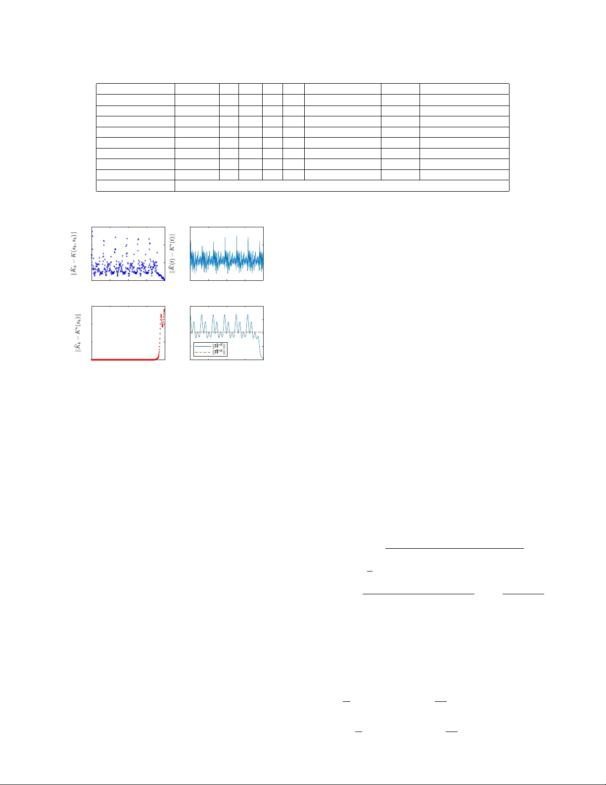
1 Adapti v e Optimal Control of Linear Periodic Systems: An Of f-Polic y V alue Iteration Approach Bo Pang, Student Member , IEEE , and Zhong-Ping Jiang, F ellow , IEEE Abstract —This paper studies the infinite-horizon adaptiv e op- timal control of continuous-time linear periodic (CTLP) systems. A novel v alue iteration (VI) based off-policy ADP algorithm is proposed f or a general class of CTLP systems, so that approximate optimal solutions can be obtained directly from the collected data, without the exact knowledge of system dynamics. Under mild conditions, the proofs on unif orm conver gence of the pr oposed algorithm to the optimal solutions are given for both the model-based and model-free cases. The VI-based ADP algorithm is able to find suboptimal controllers without assuming the knowledge of an initial stabilizing controller . Application to the optimal control of a triple inverted pendulum subjected to a periodically varying load demonstrates the feasibility and effectiveness of the proposed method. Index T erms —Adaptive dynamic programming, linear periodic systems, optimal control, value iteration. I . I N T R O D U C T I O N Recently , reinforcement learning (RL) has inv oked a lot of research interests from both researchers in academia and practitioners in industry , due to its successful applications to the design of intelligent computer GO player and many other intelligent agents learning tasks [1]. In RL, agents (or controllers) find optimal decisions (controls) from scratch through its interactions with an unknown en vironment. In spite of its popularity , most previous RL algorithms hav e their o wn limitations. Firstly , the underlying en vironments are described by Markov decision processes [1], where time is discrete and the state and input spaces are finite or countable. Secondly , stability and safety properties associated with the use of the obtained optimal polic y are not considered and guaranteed. Howe ver , man y physical systems are more naturally described by differential equations, where time is continuous and the state and input spaces are infinite and continuous. Stability and safety are also indispensable considerations in real-world applications, e.g., autonomous vehicles. T o this end, ov er the past decade, another stream of RL algorithms has emer ged, to solve the optimal control problems described by dif ferential equations, without the exact kno wledge of the system dy- namics, and with stability guarantees; see, e.g., [2], [3] and numerous references therein. This class of RL algorithms are often coined adaptiv e dynamic programming (ADP), to be distinguished from those with Markov decision processes. The This work was partially supported by the National Science Foundation under Grants ECCS-1501044 and EPCN-1903781. The authors are with the Control and Networks Lab, Department of Electri- cal and Computer Engineering, T andon School of Engineering, Ne w Y ork Uni- versity , 370 Jay Street, Brooklyn, NY 11201, USA (e-mail: bo.pang@n yu.edu; zjiang@nyu.edu). interested reader can consult the books [2], [4] for sev eral practical applications of ADP . While significant progresses have been made in the de- velopment of ADP , most of the existing results are devoted exclusi vely to time-in v ariant systems. When problems arise from applications in volving time-v arying control systems, those ADP algorithms previously dev eloped for time-in variant systems are not directly applicable. Recently , in [5] and [6], the finite-horizon optimal control problem was studied for time- varying systems by ADP . Howe ver , the corresponding infinite- horizon optimal control problem for time-v arying systems de- scribed by dif ferential equations has receiv ed scanty attention. There are se veral technical obstacles for this generalization. First, the stability analysis and control synthesis of time- varying systems are much more challenging than the case of time-in variant systems. Second, predicting the future ev olution of the system trajectories becomes an intractable task for general time-v arying systems, using only the historical data collected ov er a finite period of time, which is a ke y to the dev elopment of ADP algorithms. W ith these observ ations in mind, ho w to de velop ADP algorithms to address the infinite- horizon optimal control problem of uncertain time-varying systems with guaranteed stability remains an open problem. In this paper, we take a step forward to study this longstanding unresolved issue. T o this end, we will examine the infinite- horizon adaptiv e optimal control of continuous-time linear periodic (CTLP) systems. The analysis and control of linear period systems ha ve played an important role in various applications. By exploiting the periodic time-varying nature, vibration is significantly acti vely suppressed in wind turbine system [7] and rotor-blade system [8]; through the design of periodic model predictiv e control strategies for periodic systems, better economic performance is achiev ed in building climate control [9], drinking water network [10] and noniso- lated microgrid [11]; periodic feedback controller is reported to outperform a standard time-inv ariant feedback controller in online advertising [12]; to name a few . Orbital stabilization of time-in v ariant nonlinear systems can also be analyzed and designed using linear periodic systems, since linearization of nonlinear systems along a periodic orbit yields linear periodic systems [13, Section 5.1]. It should be emphasized that ev en for the class of CTLP systems, the design of ADP algorithm is a non-tri vial task, as a result of the nonlinear dependence of system parameters on the time. Inspired by the time-in variant results in [14], a novel value iteration (VI) based ADP algorithm is proposed for a class of CTLP systems in this paper , to find approximate optimal controllers without the exact knowledge of system dynamics 2 and an initial stabilizing controller . The VI-based ADP is based on the asymptotic property of finite-horizon solution of the periodic Riccati equation (PRE). It is claimed in [15] that the solution of the PRE starting from a positi ve semidefinite initial matrix conv erges to the stabilizing solution of the same PRE, under certain conditions. Howe ver , it is pointed out by the authors of [16] and [17] that the proof of the claim in [15] is based on some wrong preliminary results (see Remark 1). In the present paper , we firstly gi ve a new proof of the claim, and then present a VI-based ADP algorithm, using the Fourier basis approximation. It turns out that the VI- based ADP algorithm amounts to numerically solving the final value problem of a nonlinear differential equation, which only inv olves collected data and is independent of the exact system dynamics. In Section III, the uniform con vergence of the VI-based ADP algorithm to the optimal solution of the corresponding optimal control problem is rigorously pro ved. In Section IV, the proposed VI-based ADP algorithm is applied to the adaptiv e optimal control of a triple in verted pendulum subjected to a periodically varying load, which demonstrates the effecti veness of the resulting algorithm. Section V closes the paper with some concluding remarks. It is worth noting that there is a rich literature on optimal control (see, e.g., [7]–[11]) and on adaptive control (see, e.g., [18]–[20]) for linear periodic systems. Howe ver , they ha ve been studied as two separate problems. That is, the optimal control solutions presented in [7]–[11] require the precise knowledge of the system dynamics, while the adaptiv e control results presented in [18]–[20] do not guarantee optimization of any prescribed cost function. Dif ferent from both groups of research, our proposed method finds the suboptimal solutions directly from the input/state data, without the exact knowledge of the system dynamics. Notations : R ( R + ) is the set of (nonne gati ve) real num- bers. Z + is the set of nonnegati ve integers. S n denotes the vector space of all n -by- n real symmetric matrices. ⊗ is the Kronecker product operator . | · | and k · k represent the Euclidean norm for vectors and the Frobenius norm for matrices, respectiv ely . [ v ] j denotes the j th element of vector v ∈ R n . [ X ] i,j denotes the element in i th row and j th column of matrix X ∈ R m × n . b v c represents the lar gest integer no larger than v ∈ R . X † denotes the Moore-Penrose inv erse of matrix X . σ min ( X ) is the minimal singular v alue of matrix X . I I . P RO B L E M F O R M U L AT I O N A N D P R E L I M I NA R I E S Consider continuous-time linear periodic systems ˙ x ( t ) = A ( t ) x ( t ) + B ( t ) u ( t ) , (1) where x ( t ) ∈ R n is the system state, u ( t ) ∈ R m is the control input, A ( · ) : R → R n × n , B ( · ) : R → R n × m are continuous and T -periodic matrix-valued functions, i.e., A ( t + T ) = A ( t ) , B ( t + T ) = B ( t ) , T ∈ R + , ∀ t ∈ R . Let Φ( t, t 0 ) , t > t 0 , t 0 ∈ R denote the state transition matrix of the unforced system of (1), with u = 0 . In the setting of linear periodic system, the matrix Φ( t 0 + T , t 0 ) is known as the monodromy matrix. Its eigen v alues (also called characteristic multipliers) are independent of t 0 . A ( · ) is asymptotically stable if and only if its characteristic multipliers are inside the open unit disk. See [21] for the details. The infinite-horizon periodic linear quadratic (PLQ) optimal control problem [17, Section 6.5.1.1] is to find a linear stabiliz- ing control law u ( t ) = − K ( t ) x ( t ) , where K ( · ) : R → R m × n is continuous and T -periodic, such that the follo wing quadratic cost is minimized J ( t 0 , ξ , u ( · )) = Z ∞ t 0  | C ( t ) x ( t ) | 2 + u T ( t ) R ( t ) u ( t )  dt, (2) where C ( · ) : R → R r × n is continuous and T -periodic; R ( · ) : R → R m × m is continuous, T -periodic, positi ve definite and piecewise continuously differentiable; x ( t ) is the solution of (1) with initial state x ( t 0 ) = ξ , ξ ∈ R n . Associated with the PLQ control problem is the PRE − ˙ P ( t ) = A T ( t ) P ( t ) + P ( t ) A ( t ) − P ( t ) B ( t ) R − 1 ( t ) B T ( t ) P ( t ) + C T ( t ) C ( t ) . (3) Generally , the PRE (3) may admit many different kinds of solutions, among which two particular kinds are relev ant to this paper . Definition 1 ( [17], [22]) . Consider the r eal symmetric, periodic and positive semidefinite (SPPS) solutions satisfying PRE (3) over time interval ( −∞ , ∞ ) . 1) P S ( · ) is called strong solution, if the characteristic multi- pliers of D S ( t ) = A ( t ) − B ( t ) R − 1 ( t ) B T ( t ) P S ( t ) belong to the closed unit disk. 2) P + ( · ) is called stabilizing solution, if the characteristic multipliers of D + ( t ) = A ( t ) − B ( t ) R − 1 ( t ) B T ( t ) P + ( t ) belong to the open unit disk. Assumption 1. ( A ( · ) , B ( · )) is stabilizable and ( A ( · ) , C ( · )) is detectable [21, Theor em 4]. Under Assumption 1, the optimal solution to the infinite- horizon PLQ control problem exists and is unique [17, Theo- rem 6.5 and 6.12]. Lemma 1. Ther e e xists a unique SPPS solution P ∗ ( · ) of the PRE, and the corr esponding closed-loop system is stable, if and only if Assumption 1 is satisfied. In ad- dition, a) P S = P + = P ∗ . b) the cost (2) is mini- mized by the optimal controller u ∗ ( t ) = − K ∗ ( t ) x ( t ) , with K ∗ ( t ) = R − 1 ( t ) B T ( t ) P ∗ ( t ) . c) the corr esponding minimum cost is J ∗ ( t 0 , ξ ) = J ( t 0 , ξ , u ∗ ( · )) = ξ T P ∗ ( t 0 ) ξ . In general, it is difficult to obtain an analytic expression for P ∗ ( · ) , which is a nonlinear matrix-v alued function of time t . In this paper , Fourier basis functions are adopted to approximate different periodic functions. For a continuous and T -periodic function f ( · ) : R → R , partial sums of its Fourier series representation are f N ( x ) = a 0 2 + N X i =1 ( a i cos ( ω ix ) + b i sin ( ω ix )) , where ω = 2 π /T , N ∈ Z + , { a i } N i =0 and { b i } N i =1 are Fourier coef ficients. The follo wing lemma gi ves the asymptotic property of using f N to approximate f . 3 Lemma 2 ( [23, Theorem 1.5.1]) . If f is T -periodic, contin- uous and piecewise continuously dif fer entiable, then f N → f uniformly , as N → ∞ . When matrices A ( · ) and B ( · ) are unknown, the optimal solution P ∗ ( · ) can hardly be obtained directly due to the nonlinearity of the PRE. In next section, VI is exploited to find approximate optimal controllers directly from the input/state data collected along the controlled system trajectories. As it can be directly checked, we have Fact 1. F or X ∈ R n × m , Y ∈ S n , v ∈ R n , | v ec( X ) | = k X k , | vecs( Y ) | = k Y k , v T Y v ≡ ˜ v T v ecs( Y ) , wher e v ec( X ) = [ X T 1 , X T 2 , · · · , X T m ] T , v ecs( Y ) = [ y 11 , √ 2 y 12 , · · · , √ 2 y 1 m , y 22 , √ 2 y 23 , · · · , √ 2 y m − 1 ,m , y m,m ] T ∈ R 1 2 m ( m +1) , ˜ v = [ v 2 1 , √ 2 v 1 v 2 , · · · , √ 2 v 1 v n , v 2 2 , √ 2 v 2 v 3 , · · · , √ 2 v n − 1 v n , v 2 n ] T ∈ R 1 2 n ( n +1) , X i is the i th column of X . In addition, ther e always exist oper - ations vec − 1 ( · ) and vecs − 1 ( · ) , such that X = vec − 1 (v ec( X )) and Y = vecs − 1 (v ecs( Y )) , respectively . I I I . V A L U E I T E R A T I O N B A S E D A D A P T I V E D Y NA M I C P R O G R A M M I N G F O R C O N T I N U O U S - T I M E L I N E A R P E R I O D I C S Y S T E M S The value iteration method is based on the asymptotic property of the solution to the finite-horizon PLQ optimal control problem. For any t < t f and a measurable locally essentially bounded input u : [ t, t f ) → R m , define finite- horizon cost V ( t, t f , ξ , u ( · ) , G ) = x ( t f ) T Gx ( t f ) + Z t f t  | C ( t ) x ( t ) | 2 + u ( t ) T R ( t ) u ( t )  dt, for all ξ ∈ R n and G ∈ S n , G ≥ 0 , where x ( t ) = ξ . Starting at P ( t f ) = G , the corresponding solution of the PRE (3) at time t < t f , denoted by P ( t ; t f , G ) , satisfies ξ T P ( t ; t f , G ) ξ = min u V ( t, t f , ξ , u ( · ) , G ) . Generally , P ( · ; t f , G ) is not necessarily periodic, and different from the SPPS solutions in Definition 1, P ( · ; t f , G ) satisfies PRE (3) over time interval ( −∞ , t f ] [24, Section 6.1.4]. Next, it is sho wn that P ( t ; t f , G ) with G ≥ 0 will approach the SPPS solution P ∗ ( t ) of the PRE (3), as time t → −∞ . Lemma 3. F or any 0 ≤ G 1 ≤ G 2 and t < t f , P ( t ; t f , G 1 ) ≤ P ( t ; t f , G 2 ) . Pr oof. For any fixed ξ ∈ R n , and any measurable locally essentially bounded u , ξ T P ( t ; t f , G 1 ) ξ ≤ V ( t, t f , ξ , u, G 1 ) ≤ V ( t, t f , ξ , u, G 2 ) . Minimizing the abo ve inequalities simultaneously over u , we obtain ξ T P ( t ; t f , G 1 ) ξ ≤ ξ T P ( t ; t f , G 2 ) ξ . Since ξ is arbitrary , the proof is completed. Theorem 1. Under Assumption 1, if G = G T ≥ 0 , then lim t →−∞ ( P ( t ; t f , G ) − P ∗ ( t )) = 0 . (4) Pr oof. See the Appendix. Remark 1. In 1975, Hewer dr ew the same conclusion [15, Theor em 4.11] with Theorem 1. However , as pointed out in [17, Section 6.3.4] and [16], the pr oof of [15, Theorem 4.11] was based on [15, Theor em 3.7], which is shown wr ong by a counter example in [16, Section 2]. The proof of Theorem 1 in this paper is new and is included for the sake of completeness. Note that the solutions of PRE (3) need not e volv e according to the same time variable in system (1). T o emphasize this point, in the rest of this paper we use s ∈ R for the algorithmic time, which is the time used in the PRE, while t ∈ R is reserved for the system ev olution time, i.e. the time used in system (1). This separation of time variables is essential in the dev elopment of our proposed algorithm in the sequel (also see Remark 4). Theorem 1 means that near-optimal solutions of P ∗ ( · ) can be found by solving the PRE (3) backward in time with boundary condition G ≥ 0 . Concretely , we can solve the following final value problem on interval [0 , s f ] , − ˙ P ( s ) = A T ( s ) P ( s ) + P ( s ) A ( s ) + C T ( s ) C ( s ) − P ( s ) B ( s ) R − 1 ( s ) B T ( s ) P ( s ) , P ( s f ) = G, (5) where G = G T ≥ 0 , P ( s ) is short for P ( s ; s f , G ) . By Theorem 1, if s f > 0 is large, then P ( s ) is close to P ∗ ( s ) for s near 0 . Ho we ver , the a priori knowledge of A ( · ) and B ( · ) is still required to solve (5). Next, a VI-based off-polic y ADP algorithm is proposed to solve (5) directly from input/state data, without the exact knowledge of A ( · ) and B ( · ) . Define matrix-valued functions H ( s, t ) = A T ( t ) P ( s ) + P ( s ) A ( t ) , K ( s, t ) = R − 1 ( t ) B T ( t ) P ( s ) . (6) Then (5) can be rewritten as, − ˙ P ( s ) = H ( s, s ) + C T ( s ) C ( s ) − K T ( s, s ) R ( s ) K ( s, s ) . (7) By Theorem 1, as long as s f is large enough, H ( s, s ) and K ( s, s ) with s near 0 will be good approximation to H ∗ ( s ) = A T ( s ) P ∗ ( s ) + P ∗ ( s ) A ( s ) , K ∗ ( s ) = R − 1 ( s ) B T ( s ) P ∗ ( s ) . (8) W ith Lemma 1, note that K ∗ ( · ) is the optimal control gain. For fixed s ∈ [0 , s f ] , H ( s, t ) and K ( s, t ) are periodic with respect to time t ∈ R . Thus we can express v ecs( H ( s, t )) and v ec( K ( s, t )) by their Fourier series v ecs( H ( s, t )) = W H ( s ) F N ( t ) + e H N ( s, t ) , v ec( K ( s, t )) = W K ( s ) F N ( t ) + e K N ( s, t ) , (9) 4 where W H ( s ) ∈ R n 1 × (2 N +1) , n 1 = n ( n + 1) / 2 and W K ( s ) ∈ R n 2 × (2 N +1) , n 2 = mn are Fourier coefficients at algorithmic time s , F N ( t ) = [1 , cos ( ω t ) , sin ( ω t ) , cos (2 ω t ) , sin (2 ω t ) , · · · , cos ( N ω t ) , sin ( N ω t )] T , e H N ( s, t ) ∈ R n 1 and e K N ( s, t ) ∈ R n 2 are truncation errors. Here is a pre view of subsequent dev elopment of our algo- rithm. W e aim at solving (5) (i.e. (7)) directly from input/state data. T o this end, firstly , using (6) and (9), the PRE (5) (i.e. (7)) is transformed into an equiv alent dif ferential equation (16), in terms of Fourier coefficients W H ( s ) and W K ( s ) . Secondly , by ignoring the truncation errors e H N ( s, t ) and e K N ( s, t ) in (16), a ne w differential equation (17) is deri ved in terms of ˆ W H ( s ) and ˆ W K ( s ) , where only input/state data is in volv ed. Thirdly , it is shown (in Lemma 6) that, ˆ W H ( s ) and ˆ W K ( s ) giv en by the new dif ferential equation (17) are close to the original Fourier coefficients W H ( s ) and W K ( s ) on [0 , s f ] under suitable conditions, despite of the ignorance of the truncation errors. This implies that the problem of solving model-based PRE (5) (i.e. (7)) on [0 , s f ] can be approached by solving the data-based differential equation (17) on [0 , s f ] . Thus then (17) is solved numerically on [0 , s f ] , and the numerical solutions with time index es near 0 are fitted by least squares to obtain two continuous functions ¯ H ( s ) and ¯ K ( s ) . Finally , these two continuous functions are sho wn (in Theorem 2) to be close to the optimal solutions H ∗ ( s ) and K ∗ ( s ) in (8), under suitable conditions. This fulfills our goal. W ith the above outline in mind, the rest of this section is dev oted to presenting the details. For M ∈ Z + \{ 0 } , define t j = j ∆ t , j = 0 , 1 , 2 , · · · , M . ∆ t is the sampling interval. Assuming a measurable locally essentially bounded input u 0 ( · ) : [0 , t M ] → R m is applied to system (1) to collect input/state data for learning, we hav e d x T ( t ) P ( s ) x ( t ) d t = ˙ x T ( t ) P ( s ) x ( t ) + x T ( t ) P ( s ) ˙ x ( t ) = x T ( t ) H ( s, t ) x ( t ) + 2 u T 0 ( t ) R ( t ) K ( s, t ) x ( t ) . (10) Integrating both sides of (10) from t j to t j +1 , by Fact 1, we obtain [ ˜ x ( t j +1 ) − ˜ x ( t j )] T v ecs( P ( s )) = Z t j +1 t j ˜ x T ( t )v ecs( H ( s, t ))d t + Z t j +1 t j  x T ( t ) ⊗ (2 u T 0 ( t ) R ( t ))  v ec( K ( s, t ))d t. (11) Using (9), we can organize (11) for j = 0 , 1 , 2 , · · · , M − 1 into a single linear matrix equation Θ " v ec( W H ( s )) v ec( W K ( s )) # + E N ( s ) = Γ ˜ x v ecs( P ( s )) , (12) where Θ =  ∆ T 0 , ∆ T 1 , · · · , ∆ T M − 1  T , ∆ j = [ I F ˜ x,j , I F xu,j ] , Γ ˜ x =  δ T 0 , δ T 1 , · · · , δ T M − 1  T , δ j = ˜ x T ( t j +1 ) − ˜ x T ( t j ) , E N ( s ) = [ e 0 ,N ( s ) , e 1 ,N ( s ) , · · · , e M − 1 ,N ( s )] T , I F ˜ x,j = Z t j +1 t j F T N ⊗ ˜ x T d t, I F xu,j = Z t j +1 t j F T N ⊗ x T ⊗ (2 u T 0 R )d t, e j,N ( s ) = Z t j +1 t j ˜ x T ( t ) e H N ( s, t ) dt + Z t j +1 t j  x T ( t ) ⊗ 2 u T 0 ( t )  e K N ( s, t )d t. (13) The following Assumption is imposed on the matrix Θ . Assumption 2. Given N > 0 , ther e exist ¯ M > ( n 1 + n 2 )(2 N + 1) and α > 0 (independent of N ), such that for all M > ¯ M , M ∈ Z + , 1 M Θ T Θ ≥ αI ( n 1 + n 2 )(2 N +1) . (14) Mor eover , for all t ∈ [0 , t M ] , | x ( t ) | ≤ β , β independent of N . Remark 2. Condition (14) appear ed in the past literatur e of ADP [2], [4], [25], which is in the spirit of persistency of excitation (PE) in adaptive contr ol. An exploration noise, such as sum of sinusoidal signals with diverse fr equencies, can be added to u 0 , if needed, to satisfy (14). Remark 3. Notice that by derivations fr om (10) to (12), in- put/state data on any time interval of length ∆ t satisfying (11) can be used to construct (12). T o fulfill condition | x ( t ) | ≤ β , one way is to r estart the system at | x ( t 0 ) | ≤ β , whenever the boundedness condition is violated. The choice of t 0 depends on the problem at hand. In r otor-blade system [8], for example , a choice of t 0 can be the moment when the angular position of the r otor is zer o. The following lemma shows that equation (12) is differen- tiable in s . Lemma 4. W H ( · ) , W K ( · ) , e H N ( · , t ) , e K N ( · , t ) and E N ( · ) in equations (9) and (12) ar e continuously differ entiable in algorithmic time s . Pr oof. From the definition (6), H ( s, t ) and ∂ s H ( s, t ) are continuous both in s and t . Then by Leibniz integral rule and the definition of Fourier coefficients, we have [ ˙ W H ( s )] i,k = 2 T Z T / 2 − T / 2 [v ecs( ∂ s H ( s, t ))] i p ( k , t ) dt, (15) where i = 1 , 2 , · · · , n 1 , k = 1 , 2 , · · · , 2 N + 1 and p ( k , t ) =      1 , if k = 1 cos ( ω tk / 2) , if k is e ven sin ( ω t b k / 2 c ) , if k is odd and k > 1 . Thus by [26, Definition 10.1], W H ( · ) is continuously dif feren- tiable in s . By (9), e H N ( · , t ) is continuously differentiable in s . 5 W ith similar ar guments, we kno w that W K ( · ) and e K N ( · , t ) are continuously dif ferentiable in s . Note that e H N ( s, t ) , e K N ( s, t ) , ∂ s e H N ( s, t ) and ∂ s e K N ( s, t ) are continuous both in s and t . Again, by Leibniz integral rule, (13) and [26, Definition 10.1], E N ( · ) is continuously differentiable in s . This completes the proof. By Lemma 4, equations (7) and (9), and Assumption 2, taking deriv ativ es with respect to s on both sides of (12), we hav e " v ec( ˙ W H ( s )) v ec( ˙ W K ( s )) # = H ( W ( s ) , s ) + G ( W ( s ) , s ) , (16) where H ( W ( s ) , s ) = Θ † Γ ˜ x  − W H ( s ) F N ( s ) − v ecs( C T ( s ) C ( s )) +v ecs  (v ec − 1 ( W K ( s ) F N ( s ))) T R ( s ) v ec − 1 ( W K ( s ) F N ( s ))  , G ( W ( s ) , s ) = Θ † h − ˙ E N ( s ) +Γ ˜ x  v ecs  (v ec − 1 ( W K ( s ) F N ( s ))) T R ( s )vec − 1 ( e K N ( s, s )) +(v ec − 1 ( e K N ( s, s ))) T R ( s )vec − 1 ( W K ( s ) F N ( s )) +(v ec − 1 ( e K N ( s, s ))) T R ( s )vec − 1 ( e K N ( s, s ))  − e H N ( s, s )  , W ( s ) = h  W H ( s )  T ,  W K ( s )  T i T . In (16), all the terms containing the truncation errors are grouped into G ( W ( s ) , s ) . If G ( W ( s ) , s ) is ignored, we obtain the following differential equation " v ec( ˙ ˆ W H ( s )) v ec( ˙ ˆ W K ( s )) # = H  ˆ W ( s ) , s  , ˆ W ( s f ) = 0 . (17) where ˆ W ( s ) =   ˆ W H ( s )  T ,  ˆ W K ( s )  T  T . Notice that no explicit system dynamics information is con- tained in (17). Thus if ˆ W ( s ) is close to W ( s ) , approximate optimal controllers are possible to be found in view of (9), directly from the collected data. Indeed, the following two lemmas show that ˆ W ( s ) can be made close to W ( s ) . Remark 4. Thr ough the derivations fr om (5) to (17), equation (10) is a critical step in getting rid of the knowledge of system dynamics. The validity of (10) is a result of distinguishing the algorithmic time s fr om the system evolution time t . This justifies the importance of the separation of time variables. Assumption 3. The matrix-valued functions A ( · ) and B ( · ) ar e T -periodic and continuously dif fer entiable on R . Lemma 5. Under Assumptions 1, 2 and 3, for any −∞ < s 0 < s f : 1) e H N ( s, t ) , e K N ( s, t ) , ∂ s e H N ( s, t ) , ∂ s e K N ( s, t ) all conver ge uniformly to 0 on [ s 0 , s f ] × R , as N → ∞ . 2) for any  > 0 , there exists ¯ N > 0 , such that ∀ N > ¯ N , sup s ∈ [ s 0 ,s f ] |G ( W ( s ) , s ) | < . Pr oof. See the Appendix. Lemma 6. Let G = 0 in PRE (5). Under Assumptions 1, 2 and 3, for any  > 0 and 0 < s f < ∞ , there exists ¯ N > 0 , such that ∀ N > ¯ N , sup s ∈ [0 ,s f ] k W H ( s ) − ˆ W H ( s ) k < , sup s ∈ [0 ,s f ] k W K ( s ) − ˆ W K ( s ) k < . Pr oof. See the Appendix. W ith Lemma 6, we can solve equation (17) by any con- ver gent numerical method [27, Section 213] backward in time on [0 , s f ] , to find approximate values of W ( s ) . Supposing in the numerical method, the step size is h , and at step values { s k } L k =0 , s k = kh , hL = s f , the numerical solutions of (17) are computed, denoted by { ˆ W H k } L k =0 and { ˆ W K k } L k =0 . Then we can define v ecs( ˆ H k ) = ˆ W H k F N ( s k ) , vec( ˆ K k ) = ˆ W K k F N ( s k ) , (18) which are used as approximations to H ( s, s ) and K ( s, s ) at { s k } L k =0 , respectiv ely . But (18) is discrete, which is not con venient. So we would like to fit the part of the data close to (8) in (18) to get two continuous functions ¯ H ( · ) and ¯ K ( · ) . Supposing we are able to choose a ¯ L ∈ Z + , satisfying s ¯ L > T and b L/ 2 c > ¯ L > 2 N + 1 , define U = h F N ( s 0 ) F N ( s 1 ) · · · F N ( s ¯ L ) i T , V = h v ecs( ˆ H 0 ) v ecs( ˆ H 1 ) · · · vecs( ˆ H ¯ L ) i T , W = h v ec( ˆ K 0 ) v ec( ˆ K 1 ) · · · vec( ˆ K ¯ L ) i T . Assumption 4. Given N > 0 , there e xist b L/ 2 c > ¯ L 0 > 2 N + 1 and α > 0 (independent of N ), such that for all b L/ 2 c > ¯ L > ¯ L 0 , s ¯ L > T , 1 ¯ L U T U ≥ αI 2 N +1 . Under Assumption 4, over -determined least squares fittings are implemented on data sets {V , U } and {W , U } , respec- tiv ely , to get ¯ H ( t ) = vecs − 1 ( ¯ W H F N ( t )) , ¯ K ( t ) = v ec − 1 ( ¯ W K F N ( t )) , (19) where ( ¯ W H ) T = U † V , ( ¯ W K ) T = U † W . (20) W e are in a position to state our main result on approximating the optimal solution of the infinite-horizon PLQ problem without the precise knowledge of system dynamics. Theorem 2. Consider the infinite-horizon PLQ optimal con- tr ol pr oblem of system (1) with cost ( 2 ). Under Assumptions 1, 2, 3 and 4, for any  > 0 , ther e exist ¯ s f > 0 , ¯ N > 0 , ¯ h > 0 , such that ∀ s f > ¯ s f , ∀ N > ¯ N , any 0 < h < ¯ h , we have sup t ∈ R k ¯ H ( t ) − H ∗ ( t ) k < , sup t ∈ R k ¯ K ( t ) − K ∗ ( t ) k < , wher e ¯ L is chosen to satisfy s ¯ L > T , b L/ 2 c > ¯ L > 2 N + 1 . 6 Pr oof. See the Appendix. T o sum up, our novel VI-based off-policy ADP algorithm is presented in Algorithm 1. Algorithm 1: VI-based off-policy ADP Choose ∆ t > 0 , large enough M > 0 , N > 0 , s f > 0 , and small enough h > 0 . Apply u 0 ( · ) : [0 , t M ] → R m (with exploration noise) to system (1), collect the input/state data. Construct the data matrices Θ and Γ ˜ x . Solve numerically (17) backward in time on [0 , s f ] . Choose ¯ L satisfying s ¯ L > T , b L/ 2 c > ¯ L > 2 N + 1 . Solve (19) for ¯ K ( t ) . Use ¯ u ( t ) = − ¯ K ( t ) x ( t ) as the approximate optimal control for all t ∈ [0 , ∞ ) . Lem mas 2, 5, 6       󰇛    󰇜       󰇛  󰇜         󰇛  󰇜          󰇛  󰇜    󰇛  󰇜   󰇛  󰇜    󰇛  󰇜 ( 9) Lem ma 6 (2 0 ) ( 19) The or em 2 The or em 1 Lem ma 5 Lem mas 1, 3 Lem ma 2 (1 2) ( 16) Lem ma 4 Fig. 1. Overview of deriv ations and conver gence analysis of Algorithm 1. T o giv e a clearer explanation of the deriv ations and con ver- gence analysis of Algorithm 1, the relationships of different components in this section are summarized in Figure 1. Remark 5. In (6) and (9), if lim s →−∞ P ( s ) − P ∗ ( s ) = 0 , W ( s ) will conver ge to a unique periodic orbit. In view of Lemma 6, ˆ W ( s ) will be close to that periodic orbit. This suggests a heuristic pr ocedure for the choice of parameters in Algorithm 1: (1) Choose some ∆ t > 0 , N > 0 . (2) In view of Assumption 2, Θ should be at least full column rank. Thus M  ( n 1 + n 2 )(2 N + 1) . Then t M = M ∆ t . (3) F ind an s f , such that k ˆ W ( s ) k given by (17) is almost periodic near s = 0 . If such an s f can not be found for lar ge values of s f , incr ease N and go back to step (2). (4) Set h > 0 such that b s f h c  2 N + 1 . (5) Choose ¯ L satisfying s ¯ L > T , b L/ 2 c > ¯ L > 2 N + 1 . I V . S I M U L A T I O N R E S U LT S Consider the triple in verted pendulum with a periodically varying load [28], modeled by system (1) with A ( t ) = " 0 3 I 3 A 21 ( t ) A 22 # , B ( t ) = " 0 3 B 2 # (21) A 21 ( t ) =    ( γ − 3) (3 − γ ) − 1 (4 − γ ) 2( γ − 3) (3 − γ ) − 1 (4 − γ ) ( γ − 3)    , A 22 = 0 . 5    − 1 0 0 1 − 1 0 0 1 − 1    , B 2 =    1 − 1 0 − 1 2 − 1 0 − 1 2    , and states x ( t ) = [ η 1 ( t ) , η 2 ( t ) , η 3 ( t ) , ˙ η 1 ( t ) , ˙ η 2 ( t ) , ˙ η 3 ( t )] T , inputs u ( t ) = [ u 1 ( t ) , u 2 ( t ) , u 3 ( t )] T , where γ = 1 + 2 cos ( t ) . For each i = 1 , 2 , 3 , η i ( · ) is the angle of the i th pendulum with respect to the vertical line; ˙ η i ( · ) is the corresponding angular velocity; u i ( · ) is the control torque applied at the bottom of the i th pendulum. If the system matrices in (21) are kno wn, (5) can be solv ed to obtain a suboptimal controller, which is referred as model- based PLQ (MBPLQ) controller . Howe ver , the actual system need not ev olve e xactly as (21). Suppose an e xtra periodically varying disturbance exists, which changes A 21 ( t ) in (21) to ˜ A 21 ( t ) = A 21 ( t ) + ζ (1 + sin (3 t )) I 3 , where ζ > 0 controls the magnitude of the disturbance. Algorithm 1 is applied to (21) with ˜ A 21 ( t ) , to obtain ADP controllers. The simulation results with different choices of controllers, N , M , s f and ζ are summarized in T able I. It is easy to check that Assumptions 1 and 3 are satisfied by system (21) and the choice of C ( · ) in T able I. In the simulation trials of ADP controllers, the following initial controller [ u 0 ( t )] i = 0 . 2 ∗ 500 X j =1 sin ( ω i,j t ) , i = 1 , 2 , 3 is applied to the system ov er time interval [0 , t M ] to collect data, where ω i,j is drawn from a uniform distribution ov er [ − 500 , 500] . T o guarantee the collected data is bounded, we reset x ( t j ) to the initial state x ( t 0 ) = 0 , t 0 = 0 as long as | x ( t j ) | > 10 . In T able I, trial 1 yields the best result. Loss of stability and/or optimality occurs when one of the parameters N , M , s f is not large enough, as shown in trials 2-6. Although MBPLQ controller is robust to extra disturbance with small magnitude in Trial 7, it is not robust to extra disturbance of large magnitude in trial 8, in contrast to the ADP controller . The different control gains generated by Algorithm 1 in trial 1 are compared with the optimal gains in Fig. 2. These simulation results demonstrate the viability of the theoretical results in the previous section. V . C O N C L U S I O N An innov ative VI-based ADP algorithm is proposed for CTLP systems in this paper, such that learning-based subopti- mal controllers can be obtained from real-time data without the exact knowledge of system dynamics. The proposed algorithm does not assume an initial stabilizing controller , and is of f- policy , which is easy-to-use and data-ef ficient. Con vergence analysis is developed for the presented VI-based ADP algo- rithm. It is sho wn that, under mild conditions, the proposed algorithm generates a sequence of suboptimal controllers con verging uniformly to the optimal solutions. In addition, the proposed adaptive optimal control method is successfully tested in a benchmark example of controlling a triple in verted pendulum with a periodically v arying load. Our future work can be directed at extending the proposed methodology to the optimal output regulation problem as shown in [25]. 7 T ABLE I S I MU LAT I O N R E S U L T S O F T H E T RI P L E I N V E RTE D P E ND UL U M C ON TR O L U N D ER DI FF E R EN T S E T T IN GS T rials Controller N M s f ζ Number of resetting Stability max t k ¯ K ( t ) − K ∗ ( t ) k 1 ADP 6 800 40 1 24 Y es 0.0498 2 ADP 3 800 40 1 24 Y es 0.8784 3 ADP 1 800 40 1 25 No 64.9159 4 ADP 6 800 12 1 25 Y es 8.1861 5 ADP 6 800 8 1 24 No 146.4805 6 ADP 6 400 40 1 13 No 151.3061 7 MBPLQ - - - 0.1 - Y es - 8 MBPLQ - - - 1 - No - Common parameters ∆ t = 0 . 2 , h = 0 . 1 , C = I 6 , R = I 3 , ¯ L = b s f / (3 h ) c . 0 10 20 30 40 Algorithmic Time 0 0.01 0.02 0.03 (a) 0 10 20 30 40 System Evolution Time 0 0.02 0.04 0.06 (b) 0 10 20 30 40 Algorithmic Time 0 5 10 15 20 (d) 0 10 20 30 40 Algorithmic Time 0 5 10 15 (c) Fig. 2. Comparison of different control gains. ¯ K ( · ) is the output of Algorithm 1; ˆ K k is defined in (18); K ( · ) is generated by model-based VI (5); K ∗ ( · ) is the optimal control gain; ˆ W K is generated by (17); ¯ W K is gi ven in (20). A C K N OW L E D G M E N T It is a pleasure to thank the Associate Editor, anonymous revie wers and T ao Bian for their helpful and constructiv e comments. A P P E N D I X A. Pr oof of Theor em 1 The proof is divided into three cases: Case 1) G > 0 ; Case 2) G = 0 ; Case 3) G ≥ 0 , G 6 = 0 with at least one zero eigen value. Case 1): In this case, by Lemma 1 and [22, Corollary], we immediately obtain lim t →−∞ ( P ( t ; t f , G ) − P ∗ ( t )) = lim t →−∞ ( P ( t ; t f , G ) − P S ( t )) = 0 . Case 2): In this case, for any t ≤ τ 1 ≤ τ 2 and any ξ ∈ R n , define u (2) ( s ) , − R ( s ) − 1 B ( s ) T P ( s ; τ 2 , 0) x (2) ( s ) , where x (2) ( s ) , t ≤ s ≤ τ 2 , is the solution of system (1) under control u (2) ( s ) . By definition, ξ T P ( t ; τ 1 , 0) ξ = min u V ( t, τ 1 , ξ , u, 0) ≤ V ( t, τ 1 , ξ , u (2) , 0) ≤ V ( t, τ 2 , ξ , u (2) , 0) = ξ T P ( t ; τ 2 , 0) ξ . Hence P ( t ; τ , 0) is nondecreasing as τ → ∞ , when t ≤ τ . By Lemma 1, P ∗ ( t ) is stabilizing solution of the PRE, which means ξ T P ∗ ( t ) ξ < ∞ , for any fixed ξ ∈ R n and t . Again, by definition, ξ T P ( t ; τ , 0) ξ ≤ V ( t, τ , ξ , u ∗ , 0) ≤ lim ¯ τ →∞ V ( t, ¯ τ , ξ , u ∗ , 0) = ξ T P ∗ ( t ) ξ < ∞ . Therefore when t ≤ τ , P ( t ; τ , 0) is nondecreasing as τ → ∞ , and bounded from the above. By the monotone conv ergence theorem, ¯ P ( t ; 0) := lim τ →∞ P ( t ; τ , 0) exists. By periodicity , P ( t + T ; τ + T , 0) = P ( t ; τ , 0) . Then we hav e ¯ P ( t + T ; 0) = lim τ →∞ P ( t + T ; τ , 0) = lim τ →∞ P ( t ; τ , 0) = ¯ P ( t ; 0) . Furthermore, P ( t ; τ , 0) is symmetric and positi ve semidefinite for all t ≤ τ . This implies that ¯ P ( t ; 0) is a SPPS solution of the PRE. Due to the uniqueness of the SPPS solution, we hav e ¯ P ( t ; 0) = P ∗ ( t ) . In P ( t ; τ , 0) , τ → ∞ is equiv alent to t → −∞ , thus (4) holds when G = 0 . Case 3): In this case,we can always find a ¯ G > 0 , such that 0 ≤ G ≤ ¯ G , then (4) follows by Lemma 3 and the squeeze theorem [29, Theorem 3.3.6]. B. Pr oof of Lemma 5 For 1), by Assumption 3, A ( t ) is locally Lipschitz contin- uous at t , hence A ( · ) is Lipschitz continuous on compact set [ t, t + T ] . Due to the periodicity , we know that A ( · ) is Lipschitz continuous on R . Define F ( s, τ ) = v ecs( H ( s, t − τ )) − vecs( H ( s, t )) sin( ω τ / 2) for 0 < | τ | ≤ T 2 , and put F ( s, 0) = 0 . Then we have |F ( s, τ ) | ≤ 2 k A ( t − τ ) − A ( t ) kk P ( s ) k | sin( ω τ / 2) | ≤ ¯ U     τ sin( ω τ / 2)     , where ¯ U > 0 does not depend on t , s or τ , since A ( · ) is Lipschitz continuous on R and P ( s ) is bounded by Theorem 1. From above inequalities, it is easy to see that |F ( s, τ ) | is bounded on [ s 0 , s f ] × [ − T / 2 , T / 2] . Follo wing the same deriv ations as those in [26, Theorem 8.14], we have W H ( s ) F N ( t ) − vecs( H ( s, t )) = 1 T Z T / 2 − T / 2 h F ( s, τ ) cos( ω τ 2 ) i sin( N ω τ )d τ + 1 T Z T / 2 − T / 2 h F ( s, τ ) sin( ω τ 2 ) i cos( N ω τ )d τ , 8 which con verges uniformly on [ s 0 , s f ] × R to 0 as N → ∞ , as a result of [26, Theorem 8.12] and the boundedness of F ( s, τ ) . Therefore, lim N →∞ e H N ( s, t ) = 0 uniformly on [ s 0 , s f ] × R . Through similar arguments, we can prove that e K N ( s, t ) , ∂ s e H N ( s, t ) , ∂ s e K N ( s, t ) all con verge uniformly to 0 on [ s 0 , s f ] × R . For 2), by definition of G ( W ( s ) , s ) , Lemma 2 and As- sumption 2, for any  0 > 0 , there exists ¯ N 0 > 0 , such that ∀ N > ¯ N 0 , sup s ∈ [ s 0 ,s f ] |G ( W ( s ) , s ) | < M k Θ † k 2 (1 + 2 β 4 )  0 = M (1 + 2 β 4 ) σ min (Θ)  0 ≤ 1 + 2 β 4 α  0 . Note that α and β are independent of N , the proof is completed. C. Pr oof of Lemma 6 Firstly , we pro ve that if the solution of (17) e xists on interv al [ s 0 , s f ] , for some −∞ < s 0 < s f and ∀ N > N 1 , N 1 > 0 , then Lemma 6 holds on this interval. Subtracting (17) from (16), we hav e " v ec( ˙ Z (1) ( s )) v ec( ˙ Z (2) ( s )) # = H ( W ( s ) , s ) − H  ˆ W ( s ) , s  + G ( W ( s ) , s ) , (22) where Z ( s ) = " Z H ( s ) Z K ( s ) # = " W H ( s ) − ˆ W H ( s ) W K ( s ) − ˆ W K ( s ) # , Z ( s f ) = 0 . Consider the following differential equation ev olving on [ s 0 , s f ] " v ec( ˙ Z H 0 ( s )) v ec( ˙ Z K 0 ( s )) # = H ( W 0 ( s ) , s ) − H  ˆ W 0 ( s ) , s  , (23) with Z 0 ( s f ) = 0 . Obviously , it admits a solution Z 0 ( · ) ≡ 0 . On one hand, we know from Lemma 5 that for an y  > 0 , there is some N  , such that sup s ∈ [ s 0 ,s f ] |G ( W ( s ) , s ) | <  . On the other hand, note that the RHS of (22) and RHS of (23) are locally Lipschitz in Z ( s ) and Z 0 ( s ) , respectively . Then by [30, Theorem 55], we hav e sup s ∈ [ s 0 ,s f ] k Z ( s ) k < g (  ) , (24) where g ( · ) : R + → R + is a class K ∞ function [31, Definition 4.2]. Thus, by choosing  arbitrarily small, sup s ∈ [ s 0 ,s f ] k Z ( s ) k can also be made arbitrarily small. Now , we prov e that the solution of (17) indeed exists on [0 , s f ] for N large enough. This amounts to proving that Z ( s ) exists on [0 , s f ] for N large enough, because W H ( s ) and W K ( s ) alw ays exist on ( −∞ , s f ] . F or a fixed N ∈ Z + , since the RHS of (22) is continuous in s and locally Lipschitz at Z ( s f ) = 0 , by [31, Theorem 3.1], (22) has a unique solution on [ s f − δ, s f ] , for some δ > 0 . Let ( S N , s f ] be the maximal interval of existence of (22). If S N = −∞ , then we are done. Otherwise, lim s → S + N k Z ( s ) k = ∞ . In the latter case, we claim that lim N → + ∞ S N = −∞ . T o see this, let N 1 , N 2 ∈ Z + and N 1 < N 2 . Supposing S N 1 < S N 2 , by (24) and Lemma 5, for (22) with N = N 2 , lim s 0 → S + N 2 sup s ∈ [ s 0 ,s f ] k Z ( s ) k < c , where c > 0 is some finite constant. This contradicts to the fact that S N 2 is a finite escape time for (22) with N = N 2 . Thus we can only hav e S N 1 ≥ S N 2 , i.e., { S N } ∞ N =0 is a non-increasing sequence. Assuming lim N →∞ S N = S > −∞ , we hav e lim s → S + k Z ( s ) k = ∞ . But by (24) and Lemma 5, for any S < s 0 ≤ s f , lim N →∞ sup s ∈ [ s 0 ,s f ] k Z ( s ) k ! = 0 . W e arriv e at another contradiction. Thus the only possibility is lim N → + ∞ S N = −∞ , which means the solution of (17) exists on [0 , s f ] for N large enough. The proof is thus completed. D. Pr oof of Theor em 2 For con venience, only the con vergence of ¯ H to H ∗ is prov ed. The proof on the con vergence of ¯ K to K ∗ is anal- ogous. Set G = 0 . For any  0 > 0 , by Lemma 5, there exists ¯ N 1 > 0 , such that ∀ N > ¯ N 1 , sup s ∈ [0 ,s f ] k v ecs − 1 ( W H ( s ) F N ( s )) − H ( s, s ) k <  0 4 . By Lemma 6, there exists ¯ N 2 > 0 , such that ∀ N > ¯ N 2 , sup s ∈ [0 ,s f ] | ˆ W H ( s ) F N ( s ) − W H ( s ) F N ( s ) | <  0 4 . According to [27, Theorem 213B], we can choose a ¯ h 0 , such that for all step size 0 < h < ¯ h 0 , sup k ∈{ 1 , 2 , ··· , ¯ L } | v ecs( ˆ H k ) − ˆ W H ( s k ) F N ( s k ) | <  0 4 . From Theorem 1, there exists a ¯ s f , 0 > 0 , such that ∀ s f > ¯ s f , 0 , sup s ∈ [0 ,s ¯ L ] k H ( s, s ) − H ∗ ( s ) k <  0 4 . Set ¯ N 0 = max { ¯ N 1 , ¯ N 2 } . Applying the triangle inequality to the above inequalities and by Fact 1, we obtain that, ∀ s f > ¯ s f , 0 , N > ¯ N 0 , any 0 < h < ¯ h 0 , there are sup k ∈{ 1 , 2 , ··· , ¯ L } k ˆ H k − H ∗ ( s k ) k <  0 . (25) Now define V ∗ = [v ecs( H ∗ ( s 0 )) , v ecs( H ∗ ( s 1 )) , · · · , v ecs( H ∗ ( s ¯ L ))] T , and express H ∗ ( s ) by their Fourier series, v ecs( H ∗ ( s )) = W ∗ 1 F N ( s ) + e ∗ 1 ,N ( s ) . In view of (20) and Assumption 4, we hav e ( W ∗ 1 ) T = U † ( V ∗ + E ∗ 1 ,N ) . Thus we obtain ( W ∗ 1 − ¯ W H ) T = U †  ( V ∗ − V ) + E ∗ 1 ,N  . 9 By the properties of matrix norms, we hav e 1 √ n 1 k ( W ∗ 1 − ¯ W H ) T k ≤ k ( W ∗ 1 − ¯ W H ) T k 2 ≤ kU † k 2 k  V ∗ − V ) + E ∗ 1 ,N   . By (25), Lemma 2 and Assumption 4, for any  3 > 0 , there exist large enough s f , 3 , N 3 , and small enough h 3 , such that k W ∗ 1 − ¯ W H k < √ n 1 ¯ L σ min ( U )  3 < √ n 1 α  3 . As a result of the boundedness of F N ( · ) , for any  > 0 , there exist ¯ s f > 0 , ¯ N > 0 , ¯ h > 0 , such that ∀ s f > ¯ s f , ∀ N > ¯ N , any 0 < h < ¯ h , sup t ∈ R k ¯ H ( t ) − vecs − 1 ( W ∗ 1 F N ( t )) k <  2 , sup t ∈ R k v ecs − 1 ( W ∗ 1 F N ( t )) − H ∗ ( t ) k <  2 . Again, using the triangle inequality completes the proof. R E F E R E N C E S [1] R. S. Sutton and A. G. Barto, Reinforcement Learning: An Introduction , 2nd ed. Cambridge, Massachusetts: MIT Press, 2018. [2] Y . Jiang and Z. P . Jiang, Robust Adaptive Dynamic Pro gramming . Hoboken, Ne w Jersey: W iley , 2017. [3] F . L. Lewis, D. Vrabie, and K. G. V amvoudakis, “Reinforcement learning and feedback control: Using natural decision methods to design optimal adaptive controllers, ” IEEE Control Syst. Ma g. , vol. 32, no. 6, pp. 76–105, Dec 2012. [4] F . L. Lewis and D. Liu, Eds., Reinfor cement Learning and Approximate Dynamic Pro gramming for F eedback Control . Hoboken, New Jersey: W iley-IEEE Press, 2013. [5] J. Fong, Y . T an, V . Crocher, D. Oetomo, and I. Mareels, “Dual-loop iterativ e optimal control for the finite horizon LQR problem with unknown dynamics, ” Syst. Contr ol Lett. , vol. 111, pp. 49 – 57, 2018. [6] B. Pang, T . Bian, and Z. P . Jiang, “ Adaptiv e dynamic programming for finite-horizon optimal control of linear time-varying discrete-time systems, ” Contr ol Theory T echnol. , v ol. 17, no. 1, pp. 73–84, 2019. [7] I. Houtzager , J. v an W ingerden, and M. V erhaegen, “Wind turbine load reduction by rejecting the periodic load disturbances, ” W ind Energy , vol. 16, no. 2, pp. 235–256, 2013. [8] J. Camino and I. Santos, “ A periodic linear-quadratic controller for suppressing rotor-blade vibration, ” J V ib . Control , v ol. 25, no. 17, pp. 2351 – 2364, 2019. [9] R. Gondhalekar, F . Oldewurtel, and C. N. Jones, “Least-restrictiv e robust periodic model predicti ve control applied to room temperature regulation, ” Automatica , v ol. 49, no. 9, pp. 2760–2766, 2013. [10] D. Limon, M. Pereira, D. M. De La Pe ˜ na, T . Alamo, and J. M. Grosso, “Single-layer economic model predictiv e control for periodic operation, ” J. Pr ocess Contr ol , vol. 24, no. 8, pp. 1207–1224, 2014. [11] M. Pereira, D. Limon, D. M. de la Pe ˜ na, L. V alverde, and T . Alamo, “Periodic economic control of a nonisolated microgrid, ” IEEE T rans. Ind. Electr on. , vol. 62, no. 8, pp. 5247–5255, 2015. [12] N. Karlsson, “Control of periodic sys tems in online adv ertising, ” in Pr oc. IEEE 57th Conf. Decis. Control . Miami, FL, USA: IEEE, 2018, pp. 5928–5933. [13] M. F arkas, P eriodic Motions . New Y ork: Springer Science & Business Media, 2013, vol. 104. [14] T . Bian and Z. P . Jiang, “V alue iteration, adaptiv e dynamic programming, and optimal control of nonlinear systems, ” in Pr oc. IEEE 55th Conf. Decis. Contr ol , Las V egas, NV , USA, 2016, pp. 3375–3380. [15] G. Hewer , “Periodicity , detectability and the matrix Riccati equation, ” SIAM J. Contr ol Optim. , vol. 13, no. 6, pp. 1235–1251, 1975. [16] S. Bittanti, G. Guardabassi, C. Maffezzoni, and L. Silverman, “Periodic systems: Controllability and the matrix Riccati equation, ” SIAM J. Contr ol Optim. , v ol. 16, no. 1, pp. 37–40, 1978. [17] S. Bittanti, P . Colaneri, and G. De Nicolao, “The periodic Riccati equation, ” in The Riccati Equation , S. Bittanti, A. J. Laub, and J. C. W illems, Eds. Berlin, DE: Springer, 1991, ch. 6, pp. 127–162. [18] Z. Zhang and A. Serrani, “ Adaptiv e robust output regulation of uncertain linear periodic systems, ” IEEE Tr ans. Autom. Control , vol. 54, no. 2, pp. 266–278, Feb 2009. [19] J.-X. Xu, “ A ne w periodic adaptiv e control approach for time-v arying pa- rameters with kno wn periodicity , ” IEEE T rans. Autom. Control , vol. 49, no. 4, pp. 579–583, April 2004. [20] K. S. Narendra and K. Esfandiari, “ Adaptive identification and control of linear periodic systems using second-lev el adaptation, ” Int. J. Adapt. Contr ol Signal Pr ocess. , vol. 33, no. 6, pp. 956–971, 2019. [21] S. Bittanti, “Deterministic and stochastic linear periodic systems, ” in T ime Series and Linear Systems , S. Bittanti, Ed. Berlin, DE: Springer , 1986, ch. 5, pp. 141–182. [22] G. De Nicolao, “On the conver gence to the strong solution of periodic Riccati equations, ” Int. J. Contr ol , vol. 56, no. 1, pp. 87–97, 1992. [23] D. Anton, A F irst Course in Harmonic Analysis , 2nd ed. New Y ork: Springer , 2005. [24] L. Daniel, Calculus of V ariations and Optimal Control Theory: A Concise Introduction . Princeton, New Jersey: Princeton University Press, 2012. [25] W . Gao and Z. P . Jiang, “Learning-based adaptive optimal tracking control of strict-feedback nonlinear systems, ” IEEE T rans. Neural Netw . Learn. Syst. , vol. 29, no. 6, pp. 2614–2624, June 2018. [26] W . Rudin, Principles of Mathematical Analysis . Ne w Y ork: McGraw- hill, 1976. [27] J. C. Butcher , Numerical Methods for Or dinary Differ ential Equations . Chichester , U.K.: W iley , 2016. [28] S. C. Sinha and P . Joseph, “Control of general dynamic systems with periodically varying parameters via Lyapunov-Floquet transformation, ” J. Dyn. Sys., Meas., Contr ol , vol. 116, no. 4, pp. 2439–2447, 1994. [29] H. H. Sohrab, Basic Real Analysis , 2nd ed. Ne w Y ork: Springer, 2014. [30] E. D. Sontag, Mathematical Control Theory: Deterministic F inite Di- mensional Systems , 2nd ed. Ne w Y ork: Springer, 1998. [31] H. K. Khalil, Nonlinear Systems , 3rd ed. Upper Saddle River , New Jersey: Prentice-Hall, 2002.