MPC for Humanoid Gait Generation: Stability and Feasibility

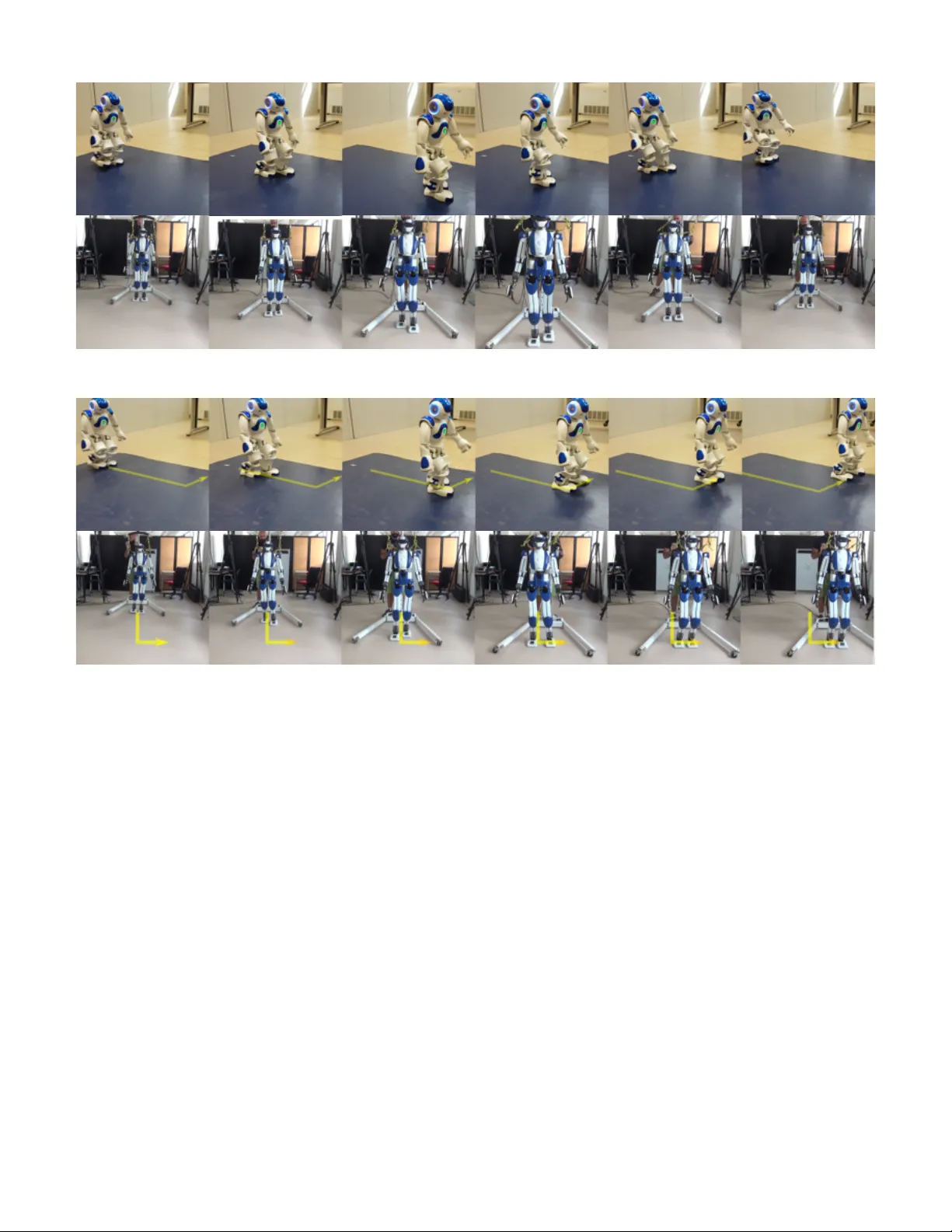
TO APPEAR IN THE IEEE TRANSA CTIONS ON R OBO TICS, 2020. DOI:10.1109/TR O.2019.2958483 1 MPC for Humanoid Gait Generation: Stability and Feasibility Nicola Scianca, Daniele De Simone, Leonardo Lanari, Giuseppe Oriolo Abstract —W e present IS-MPC, an intrinsically stable MPC framework for humanoid gait generation that incorporates a stability constraint in the formulation. The method uses as pr e- diction model a dynamically extended LIP with ZMP velocities as control inputs, producing in r eal time a gait (including f ootsteps with timing) that realizes omnidirectional motion commands coming from an external source. The stability constraint links future ZMP velocities to the current state so as to guarantee that the generated CoM trajectory is bounded with respect to the ZMP trajectory . Being the MPC control horizon ﬁnite, only part of the future ZMP velocities are decision variables; the remaining part, called tail , must be either conjectured or anticipated using pre view information on the reference motion. Several options for the tail ar e discussed, each corresponding to a speciﬁc terminal constraint. A feasibility analysis of the generic MPC iteration is developed and used to obtain sufﬁcient conditions f or recursi ve feasibility . Finally , we prove that recursi ve feasibility guarantees stability of the CoM/ZMP dynamics. Simulation and experimental results on N AO and HRP-4 are presented to highlight the perf ormance of IS-MPC. I . I N T RO D U C T I O N Many gait generation approaches for humanoids guarantee that balance is maintained during locomotion by enforcing the condition that the Zero Moment Point (ZMP , the point where the horizontal component of the moment of the ground reaction forces becomes zero) remains at all times within the support polygon of the robot. Correspondingly , these approaches identify the ZMP as the fundamental v ariable to be controlled. Due to the complexity of full humanoid dynamics, howe ver , direct control of the ZMP is very dif ﬁcult to achieve. In view of this, simpliﬁed models are generally used to relate the ev olution of the ZMP to that of the Center of Mass (CoM) of the robot, which can be instead ef fectively controlled. W idely adopted linear models are the Linear In verted Pendulum (LIP), in which the ZMP represents an input, and the Cart-T able (CT), where the ZMP appears as the output [1]. The ﬁrst is appropriate for in version-based control approaches: given a sequence of footsteps, and thus a ZMP trajectory interpolating them, the LIP is used to compute a CoM trajectory which corresponds to the ZMP trajectory; see, e.g., [2], [3], [4]. The CT model lends itself more naturally to the design of feed- back laws for tracking ZMP trajectories, the most successful example in this context being the LQ pre view controller of [5]. Regardless of the adopted model, there is a potential in- stability issue at the heart of the problem. In particular , a The authors are with the Dipartimento di Ingegneria Informatica, Automat- ica e Gestionale, Sapienza Universit ` a di Roma, V ia Ariosto 25, 00185 Rome, Italy . E-mail: { lastname } @diag.uniroma1.it. This work was supported by the European Commission through the H2020 project 645097 COMANOID. certain ZMP trajectory may be realized by an inﬁnity of CoM trajectories, which, due to the nature of the CoM/ZMP dynamics, will in general be diver gent with respect to the ZMP trajectory itself. In this situation, dynamic balance can be in principle achieved by properly choosing the ZMP trajectory , but internal instability indicates that such motion will not be feasible in practice for the humanoid. The seminal paper [6] reformulates the gait generation problem in a Model Predictiv e Control (MPC) setting. This is con venient because it allows to generate simultaneously the ZMP and the CoM trajectories while satisfying constraints, such as the ZMP balance condition as well as kinematic constraints on the maximum step length and foot rotation [7]. Moreov er , the MPC approach guarantees a certain robustness against perturbations. It is therefore not surprising that it has been adopted in many methods for gait generation; e.g., see [8], [9], [10], [11] for linear MPC and [12], [13] for nonlinear MPC. As for all control schemes, a fundamental issue in MPC approaches is the stability of the obtained closed-loop system, especially in view of the pre vious remark about the instability of the CoM/ZMP dynamics. As discussed in [14], two main approaches ha ve emerged for achieving stability when MPC is used for humanoid gait generation. The ﬁrst is heuristic in nature and consists in using a suf ﬁciently long control horizon [15], so that the optimization process can discriminate against di verging beha viors, as done for example in [7]. The second approach has been to enforce a terminal state constraint (i.e., a constraint on the state at the end of the control horizon), based on the fact that the MPC literature highlights the beneﬁcial role of such constraints for closed-loop stability in set-point control problems [16]. In particular , terminal constraints were used for humanoid balancing in [17] and for gait generation in [18]. The latter makes use of a LIP model, requiring its unstable component to stop at the end of the control horizon, a kind of terminal constraint referred to as capturability constraint (from the concept of capture point [19]). This constraint has also been used in [20], where it is imposed only at the foot landing instant, and in [21], which addresses locomotion in a multi- contact setting. Another approach focusing on the instability issue relies on the concept of Div ergent Component of Motion (DCM), used in [22] to identify an initial condition for stable execution of regular gaits, and in [23] to realize transitions between bipedal and quadrupedal gaits. The DCM concept has also been extended to the 3D context in [24], [25]. More relev ant to our re view is [26], which presents an MPC scheme for TO APPEAR IN THE IEEE TRANSA CTIONS ON R OBO TICS, 2020. DOI:10.1109/TR O.2019.2958483 2 gait generation that enforces a terminal constraint (actually con verted to a terminal cost for the sake of feasibility) on the DCM component. In this paper , we mo ve from the fundamental observ a- tion that the control problem addressed in MPC-based gait generation is neither a set-point nor a tracking problem. In fact, since the ZMP control objective is encoded via time- varying state constraints, there is no error to be regulated to (or close to) zero. The only signiﬁcant stability issue in this context is internal stability , i.e., the boundedness of the CoM trajectory with respect to the ZMP trajectory . Therefore, one cannot simply claim that the use of a terminal constraint will automatically entail internal stability . In fact, to the best of our knowledge, no MPC-based gait generation method exists in the literature for which a rigorous analysis of the stability issue has been performed in connection with the use and the choice of a terminal constraint. Another tightly related aspect to be considered is that ter- minal constraints may ha ve a detrimental ef fect on feasibility , i.e., the existence of solutions for the optimization problem which is at the core of an y MPC scheme [27]. A particularly desirable property is recur sive feasibility , which entails that if the optimization problem is feasible at a certain iteration it will remain such in future iterations. It appears that this also crucial issue has seldom been explored for MPC-based gait generation, with the notable exceptions of [28], [29]. In [30] we have introduced a novel MPC approach for humanoid gait generation which relies on the inclusion of an explicit stability constraint in the formulation of the problem. In particular , the idea was to enforce a condition on the future ZMP velocities (representing the control inputs) so as to guarantee that the generated CoM trajectory remains bounded with respect to the ZMP trajectory . Since the control horizon of the MPC algorithm is ﬁnite, only part of the future ZMP velocities are decision variables and can therefore be subject to a constraint; the remaining part, called tail , must be conjectured. Here, we fully develop our approach into a complete, Intrin- sically Stable MPC (IS-MPC) framework for gait generation. In particular , the paper adds the follo wing contributions with respect to [30]: 1) we describe a footstep generation module that can be used in conjunction with our MPC scheme in order to modify step timing and length in real time in response to omnidirectional motion commands coming from a higher - lev el module; 2) depending on the av ailable previe w information on the commanded motion, we discuss sev eral versions of the tail (truncated, periodic, anticipative) to be used in the stability constraint, and show that each of them corre- sponds to a speciﬁc terminal constraint; 3) we analyze in detail the impact of the new constraint on feasibility , and show analytically how , under certain as- sumptions, it is possibile to guarantee recursive feasibility of the IS-MPC scheme; 4) we prove that recursive feasibility of IS-MPC implies the desired internal stability of the CoM/ZMP dynamics; 5) we v alidate our ﬁndings by providing dynamic simula- tions and actual experiments on two different humanoid robots: an HRP-4 and a N A O. The results on tails, recursive feasibility and internal stabil- ity are the main contributions of this paper . W e consider them particularly important because they indicate that, contrarily to what is often claimed in the literature, simply adding a terminal constraint (e.g., the capturability constraint) does not per se guarantee stability of MPC-based gait generation schemes. Indeed, the appropriate tail to be used in the stability constraint — equi valently , the appropriate terminal constraint — depends upon the future characteristics of the commanded motion. In this sense, to guarantee recursive feasibility one should always choose the anticipativ e tail, which makes the most use of the av ailable pre view information on such motion. Once recursiv e feasibility is achiev ed, CoM/ZMP stability is automatically ensured in IS-MPC. Another potential beneﬁt of the theoretical analysis of feasibility is that it pav es the road for a formal study of the robustness of IS-MPC. Although this is out of the scope of this paper , by relying on this analysis it should be possible to devise modiﬁcations of the basic scheme which will preserve recursiv e feasibility in the presence of quantiﬁed bounded uncertainties and/or disturbances. The paper is organized as follo ws. In the ne xt section, we formulate the considered gait generation problem and discuss the structure of the proposed approach. Section III describes the algorithm which generates timing and locations of the candidate footsteps. In Sect. IV we introduce the prediction model and the constraints used in the IS-MPC scheme, with the exception of the stability constraint which is gi ven a thorough discussion in the dedicated Sect. V. The IS-MPC algorithm is described in detail in Sect. VI. Section VII addresses the central issues of stability and feasibility of the proposed method; in particular , a theoretical analysis of the feasibility of the generic IS-MPC iteration is presented and used to obtain suf ﬁcient conditions for recursi ve fea- sibility , whose role in guaranteeing stability is rigorously established. Simulations on the HRP-4 humanoid are presented in Sect. VIII, while experimental results on both the N A O and the HRP-4 humanoids are sho wn in Sect. IX. Section X offers a few concluding remarks. I I . P RO B L E M A N D A P P R OAC H Consider the problem of generating a walking gait for a humanoid in response to high-le vel reference velocities, which are giv en as the driving ( v x , v y ) and steering ( ω ) velocities of an omnidirectional single-body mobile robot chosen as a template model for motion generation. These velocities, which may encode a persistent trajectory or con ver ge to a stationary point, are produced by an external source; this could be a human operator in a shared control context, or another module of the control architecture working in open-loop (planning) or in closed-loop (feedback control). The proposed MPC-based framework, whose block scheme is shown in Fig. 1, works in a digital fashion ov er sampling intervals of duration δ . Throughout the paper , it is assumed that the reference velocities v x , v y , ω are made available for TO APPEAR IN THE IEEE TRANSA CTIONS ON R OBO TICS, 2020. DOI:10.1109/TR O.2019.2958483 3 q kinematic contr ol Intrinsicall y Sta ble MPC (IS- MPC) q dir ect kinematics candidate f oot step generatio n X f ^ k ^ k , Y f s wing f oot trajecto r y generatio n X f k k , Y f MPC-ba sed frame w ork T s k £ k f £ k f T s k v x , v y , ! o v er T p o v er T p o v er T c t k p c p swg * * p c ± T c = C ± . T p = P ± . Fig. 1. A block scheme of the proposed MPC-based framew ork for gait generation. gait generation with a pr eview horizon T p = P · δ , with P the number of intervals within the previe w horizon. At the generic instant t k = k · δ , the high-le vel references velocities over [ t k , t k + T p ] are then sent to the footstep generation module, which uses Quadratic Programming (QP) to generate candidate footsteps over the same interval. In particular, vectors ˆ X k f , ˆ Y k f collect the Cartesian positions of the footsteps, with the ‘hat’ indicating that these are candidates which can be modiﬁed by the MPC module; whereas vector Θ k f collects the footstep orientations, which will not be modiﬁed. The footstep generation module also generates the timing T k s of the sequence. The output of the footstep generation module is sent to the Intrinsically Stable MPC (IS-MPC) module, which solves another QP problem to produce in real time the actual footstep positions X k f , Y k f and the trajectory p ∗ c of the humanoid CoM ov er the contr ol horizon T c = C · δ , with C the number of intervals within the control horizon. It is assumed that T c ≤ T p , i.e., C ≤ P . The inclusion of a stability constraint in the formulation guarantees that the CoM trajectory will be bounded, in a sense to be made precise later . The pose (position and orientation) of the footsteps with the associated timing is used to generate — still in real time — the swing foot trajectory p ∗ swg ov er the control horizon. T ogether with the CoM trajectory , this is sent to the kinematic control block, which generates v elocity inputs at the joint lev el in order to achieve output tracking (we are assuming that the humanoid robot is v elocity- or position-controlled). In the next sections we will discuss in detail the proposed control scheme. W e will ﬁrst describe the footstep generation scheme, and then turn our attention to the IS-MPC algorithm, which is our core contribution. The kinematic control block can use any standard pseudoin verse-based feedback law and therefore will not be discussed further . I I I . C A N D I DA T E F O OT S T E P G E N E R AT I O N The proposed footstep generation module runs syn- chronously with the IS-MPC scheme and chooses both the timing and the candidate location of the next footsteps in response to the high-le vel reference velocities. T iming is determined ﬁrst by a simple rule expressing the fact that a change in the reference velocity should affect both the step duration and length. The candidate footstep locations are then chosen through quadratic optimization. Note that generating the timing and the orientation of the candidate footsteps outside the IS-MPC is essential to retain the linear structure of the latter . The IS-MPC scheme will still be able to adapt the position of the footsteps to guarantee reactivity to disturbances. At each sampling instant t k , the candidate footstep genera- tion module recei ves in input the high-le vel reference v eloci- ties o ver the previe w horizon, i.e., from t k to t k + T p = t k + P (see Fig. 1). In output, it provides the candidate footstep sequence ( ˆ X k f , ˆ Y k f , Θ k f ) over the same interval with the as- sociated timing T k s . In particular , these quantities are deﬁned 1 as ˆ X k f = ( x 1 f . . . x F f ) T ˆ Y k f = ( y 1 f . . . y F f ) T Θ k f = ( θ 1 f . . . θ F f ) T and T k s = { T 1 s , . . . , T F s } , where ( x j f , y j f , θ j f ) is the pose of the j -th footstep in the previe w horizon and T j s is the duration of the step between the ( j − 1) -th and the j -th footstep, taken from the start of the single support phase to the ne xt. Since the duration of steps is variable, the number F of footsteps falling within the pre view horizon T p may change at each t k . Below , we discuss ﬁrst how timing is determined and then describe the procedure for generating the candidate footsteps. A. Candidate F ootstep T iming In our method, the duration T s of each step is related to the magnitude v = ( v 2 x + v 2 y ) 1 / 2 of the reference Cartesian velocity at the beginning of that step. 1 T o keep a light notation, the k symbol identifying the current sampling instant is used for the sequence vectors but not for their individual elements. TO APPEAR IN THE IEEE TRANSA CTIONS ON R OBO TICS, 2020. DOI:10.1109/TR O.2019.2958483 4 Fig. 2. The proposed rule for determining the step duration T s as a function of the magnitude v of the reference Cartesian velocity . For comparison, also shown are the rules yielding constant step duration and constant step length. Assume that a triplet of cruise par ameters ( ¯ v , T s , ¯ L s ) has been chosen, where ¯ v is a central v alue of v and T s , ¯ L s are the corresponding v alues of the step duration and length, respectiv ely , with ¯ v = ¯ L s /T s . The choice of these parameters will depend on the speciﬁc kinematic and dynamic capabilities of the humanoid robot under consideration. The idea is that a deviation from ¯ v should reﬂect on a change in both T s and L s . In formulas: v = ¯ v + ∆ v = ¯ L s + ∆ L s T s − ∆ T s , with ∆ L s = α ∆ T s . One easily obtains T s = T s α + ¯ v α + v . (1) Figure 2 shows the resulting rule for determining T s as a function of v in comparison to other possible rules. F or illustration, we have set ¯ v = 0 . 15 m/s, T s = 0 . 8 s, ¯ L s = 0 . 12 m and α = 0 . 1 m/s. It is conﬁrmed that an increase of v , for example, corresponds to both a decrease of T s and an increase in L s . Note that the reference angular velocity ω does not enter into rule (1). The rationale is that the step duration and length along curved and rectilinear paths do not differ signiﬁcantly if the Cartesian velocity v is the same. For a purely rotational motion ( v = 0 ) where the humanoid is only required to rotate on the spot, the abov e rule would yield the maximum value of T s . In practice, equation (1) is iterated along the previe w horizon [ t k , t k + T p ] in order to obtain the footstep timestamps: t j s = t j − 1 s + T s α + ¯ v α + v ( t j − 1 s ) , with t 0 s equal to the timestamp of the last footstep before t k . Iterations must be stopped as soon as t j s > t k + P , discarding the last generated timestamp since it will be outside the previe w horizon. The resulting step timing will be T k s = { T 1 s , . . . , T F s } , with T j s = t j +1 s − t j s . B. Candidate F ootstep Placement Once the timing of the steps in the pre view horizon [ t k , t k + T p ] has been chosen, the poses of candidate footsteps are generated. T o this end, we use a reference trajectory obtained by integrating the following template model under the action of the high-le vel reference velocities ov er T p :   ˙ x ˙ y ˙ θ   =   cos θ − sin θ 0 sin θ cos θ 0 0 0 1     v x v y ω   . (2) This is an omnidirectional motion model which allows the template robot to move along any Cartesian path with an y orientation, so as to perform, e.g., lateral walks, diagonal walks, and so on. The idea is to distribute the candidate footsteps around the reference trajectory in accordance to the timing T k s while taking into account the kinematic constraints of the robot. These constraints will also be used in the IS-MPC stage, and therefore we will provide their description directly in Sect. IV -C (see also Fig. 7). A sequence of tw o QP problems is solved. The ﬁrst is          min Θ k f F X j =1 ( θ j f − θ j − 1 f − Z t j s t j − 1 s ω ( τ ) dτ ) 2 subject to | θ j f − θ j − 1 f | ≤ θ max Here, θ max is the maximum allo wed rotation between two consecutiv e footsteps. The second QP problem is          min ˆ X k f , ˆ Y k f F X j =1 ( ˆ x j f − ˆ x j − 1 f − ∆ x j ) 2 + ( ˆ y j f − ˆ y j − 1 f − ∆ y j ) 2 subject to kinematic constraints (7) Here, ( ˆ x 0 f , ˆ y 0 f ) is the known position of the support foot at t k and ∆ x j , ∆ y j are giv en by  ∆ x j ∆ y j  = Z t j s t j − 1 s R θ  v x ( τ ) v y ( τ )  dτ ± R j  0 `/ 2  , where R θ , R j are the rotation matrices associated respecti vely to θ ( τ ) (the orientation of the template robot at any given time τ ) and to the footstep orientation θ j , and ` is the reference coronal distance between consecutive footsteps. The sign of the second term alternates for left/right footsteps. At the end of this procedure, the candidate footstep se- quence ( ˆ X k f , ˆ Y k f , Θ k f ) with the associated timing T k s is sent to the IS-MPC stage. The ﬁnal footstep positions ( X k f , Y k f ) will be determined by the latter while the footstep orientations Θ k f and timing T k s will not be modiﬁed. Some examples of candidate footsteps generation are sho wn in Fig. 3. Note that the orientation of the humanoid robot is tangent to the path for the circular walk, but is kept constant ( ω = 0 ) for the other two w alks, which represent then proper examples of omnidirectional motion. I V . I S - M P C : P R E D I C T I O N M O D E L A N D C O N S T R A I N T S The IS-MPC module uses the Linear In verted Pendulum (LIP) as a prediction model. The constraints are of three kinds. The ﬁrst concerns the position of the ZMP , which must TO APPEAR IN THE IEEE TRANSA CTIONS ON R OBO TICS, 2020. DOI:10.1109/TR O.2019.2958483 5 Fig. 3. Candidate footsteps generated by the proposed method for different high-lev el reference velocities corresponding to a circular walk (top), L- walk (center), diagonal walk (bottom). The paths in black are obtained by integrating model (2) under the reference velocities. Footstep in magenta and cyan refer respectiv ely to the left and right foot. be at all times within the support polygon deﬁned by the footstep sequence and the associated timing. The second type of constraint ensures that the generated steps are compatible with the kinematic capabilities of the robot. The third is the new stability constraint guaranteeing that the CoM trajectory generated by our MPC scheme will be bounded with respect to the ZMP trajectory . The ﬁrst tw o constraints must be v eriﬁed throughout the control horizon, whereas the third is a single scalar condition on each coordinate. In this section, we discuss in detail the prediction model and the constraints on ZMP and kinematic feasibility . The next section will be de voted to the stability constraint, which deserves a thorough discussion. A. Pr ediction Model The LIP is a popular choice for describing the motion of the CoM of a biped walking on ﬂat horizontal ﬂoor when its height is kept constant and no rotational effects are present. From now on, we express motions in the robot frame, which has its origin at the center of the current support foot, the x - axis (sagittal) aligned with the support foot, and the y -axis (cor onal) orthogonal to the x -axis. In the LIP model, which CoM x c x z h c x Fig. 4. The LIP in the x direction. applies to both point feet and ﬁnite-sized feet, the dynamics along the sagittal and coronal axes are gov erned by decoupled, identical linear differential equations. Consider for illustration the motion along the x axis (see Fig. 4), and let x c and x z be respecti vely the coordinate of the CoM and the ZMP . The LIP dynamics is ¨ x c = η 2 ( x c − x z ) , (3) where η = p g /h c , with g the gra vity acceleration and h c the constant height of the CoM. In this model, the ZMP position x z represents the input, whereas the CoM position x c is the output. T o obtain smoother trajectories, we tak e the ZMP velocity ˙ x z as the actual control input. This leads to the following third-order prediction model (LIP + dynamic extension)   ˙ x c ¨ x c ˙ x z   =   0 1 0 η 2 0 − η 2 0 0 0     x c ˙ x c x z   +   0 0 1   ˙ x z . (4) Our MPC scheme uses piece wise-constant control over the sampling intervals (see Fig. 5): ˙ x z ( t ) = ˙ x i z , t ∈ [ t i , t i +1 ) . In particular , a bound of the form | ˙ x i z | ≤ γ , with γ a positiv e constant, will be satisﬁed for all i . In fact, the reference veloc- ities v x , v y , ω will be bounded in an y realistic gait generation problem. As shown by Fig. 2, the footstep generation module will then produce a sequence of footsteps along which the step duration is bounded belo w . This timing will be reﬂected in the associated ZMP constraints (see Sect. IV -B), which will in turn entail as solution a piece wise-continuous trajectory x z ( t ) with bounded deriv ative. Therefore, for t ∈ [ t i , t i +1 ] it will be x z ( t ) = x i z + ( t − t i ) ˙ x i z , with | ˙ x i z | ≤ γ , (5) where we have used the notation x i z = x z ( t i ) . The generic iteration of IS-MPC plans ov er the control horizon, i.e., from t k to t k + T c = t k + C . Since T c ≤ T p , a subset of the F candidate footsteps produced by the footstep generation module fall inside the control horizon; denote their number by F 0 < F . The MPC iteration will then generate: TO APPEAR IN THE IEEE TRANSA CTIONS ON R OBO TICS, 2020. DOI:10.1109/TR O.2019.2958483 6 x z k . t k ± t t s 1 t s 2 t s F t s F t k + C x z k + C -1 . t k + P contr ol horizon T c pr e vie w horizon T p contr ol variables x z . ~ tail x z . ’ Fig. 5. At time t k , the control variables determined by IS-MPC are the piecewise-constant ZMP velocities over the control horizon. The ZMP velocities after the control horizon are instead conjectured in order to build the tail (see Sect. V -B). Also shown are the F footstep timestamps placed by the footstep generation module in the previe w horizon; F 0 of them fall in the control horizon. • the control variables, i.e., the input values ˙ x k + i z , ˙ y k + i z , for i = 0 , . . . , C − 1 ; • the other decision variables, i.e., the actual footstep positions ( x j f , x j f ) , for j = 1 , . . . , F 0 . • as a byproduct, the output history x c ( t ) , y c ( t ) , for t ∈ [ t k , t k + C ] which will be ultimately used to driv e the actual humanoid. As already mentioned, the orientations of the footsteps are instead inherited from the generated sequence (more on this in Sect. IV -B). Note that the footsteps do not appear in the prediction model, but will show up in the constraints, as discussed in the rest of this section. B. ZMP Constraints The ﬁrst constraint guarantees dynamic balance by imposing that the ZMP lies inside the current support polygon at all time instants within the control horizon. When the robot is in single support on the j -th footstep, the admissible region for the ZMP is the interior of the footstep, which can be approximated as a rectangle of dimensions d z ,x , d z ,y , centered at ( x j f , y j f ) , and oriented as θ j . Using the fact that the ZMP proﬁle is piecewise-linear as entailed by (5), the constraint can be expressed as 2 : R T j   δ P i l =0 ˙ x k + l z − x j f δ P i l =0 ˙ y k + l z − y j f   ≤ 1 2 d z ,x d z ,y ! − R T j x k z y k z ! . (6) If the abov e sampled-time ZMP constraint is satisﬁed, then the original continuous-time constraint is also satisﬁed thanks to the linearity of x z ( t ) within each sampling interv al. Constraint (6), complete with the corresponding left-hand side, must be imposed throughout the control horizon ( i = 0 , . . . , C − 1 ) and for all the associated footsteps ( j = 0 , . . . , F 0 ). 2 For compactness, we shall only write the right-hand side of bilateral inequality constraints. For example, constraint (6) should be completed by a left-hand side obtained by adding (rather than subtracting) the two terms that appear in the right-hand side. double suppor t pol yg on d z , y d z , x j -1 j -1 ( x f , y f ) j j ( x f , y f ) ZMP admissible r egion Fig. 6. The ZMP moving constraint in double support. Note that constraint (6) is nonlinear in the footstep orienta- tion θ j , which howe ver is not a decision variable, being simply inherited from the footstep generation module. The constraint is instead linear in x j f , y j f , as well as in the ZMP velocity inputs. During double support, the support polygon would be the con vex hull of the two footsteps, whose boundary is a non- linear function of their relative position. T o preserv e linearity , we adopt an approach based on moving constraints [31]. In particular , the admissible region for the ZMP in double support has exactly the same shape and dimensions it has in single support, and it roto-translates (i.e., simultaneously rotates and translates) from one footstep to the other in such a way to always remain in the support polygon (see Fig. 6). This results in a slightly conservati ve constraint which is howe ver linear in the decision v ariables. C. Kinematic Constraints The second type of constraint is introduced to ensure that all steps are compatible with the robot kinematic limits. Consider the j -th step in T c , with the support foot centered at ( x j − 1 f , y j − 1 f ) and oriented as θ j − 1 . The admissible re gion for placing the footstep is deﬁned as a rectangle having the same orientation θ j − 1 and whose center is displaced from the support foot center by a distance ` in the coronal direction (see Fig. 7). Denoting by d a,x and d a,y the dimensions of the kinematically admissible region, the constraint can be written as R T j − 1 x j f − x j − 1 f y j f − y j − 1 f ! ≤ ± 0 ` ! + 1 2 d a,x d a,y ! , (7) with the sign alternating for the two feet. The above constraint, complete with the corresponding left-hand side, must be im- posed for all footsteps in the control horizon ( j = 1 , . . . , F 0 ). V . I S - M P C : E N F O R C I N G S TA B I L I T Y The LIP dynamics (3) is inherently unstable. As a con- sequence, even when the ZMP lies at all times within the TO APPEAR IN THE IEEE TRANSA CTIONS ON R OBO TICS, 2020. DOI:10.1109/TR O.2019.2958483 7 kinematicall y admissible r egion µ j -1 ` d k , y µ j d k , x j -1 j -1 ( x f , y f ) j j ( x f , y f ) Fig. 7. The kinematic constraint on footstep placement. support polygon (gait balance) it may still happen that the CoM diver ges e xponentially with respect to the ZMP; in this case, the gait w ould obviously become unfeasible in practice, due to the kinematic limitations of the robot. The role of the stability constraint is then to guarantee that the CoM trajectory remains bounded with respect to the ZMP (internal stability) . In this section, we ﬁrst describe the structure of the stability constraint and then discuss the possible tails for its implemen- tation. A. Stability Constraint Since we want to enforce boundedness of the CoM w .r .t. the ZMP , we can ignore the dynamic extension and focus directly on the LIP system. By using the follo wing change of coordinates x s = x c − ˙ x c /η (8) x u = x c + ˙ x c /η , (9) the LIP part of system (3) is decomposed into a stable and an unstable subsystem: ˙ x s = − η ( x s − x z ) (10) ˙ x u = η ( x u − x z ) . (11) The unstable component x u is also kno wn as diverg ent com- ponent of motion (DCM) [22] or capture point [32]. In spite of the LIP instability , for an y input ZMP trajectory x z ( t ) of the form (5) there exists a special initialization of x u such that the resulting output CoM trajectory is bounded with respect to the input [33]. In particular , this is the (only) initial condition on x u for which the free ev olution of (11) exactly cancels the component of the forced evolution that would di verge with respect to x z ( t ) . In the MPC conte xt, where the initial condition at t k is denoted by x u ( t k ) = x k u , the special initialization is expressed as x k u = η Z ∞ t k e − η ( τ − t k ) x z ( τ ) dτ . (12) Note that this particular initialization depends on the future values of the LIP input, i.e., the ZMP coordinate x z . In the following, we refer to (12) as the stability condition . The stability condition, which in volv es x u at the initial instant t k of the control horizon, can be propagated to its ﬁnal instant t k + C by integrating (11) from x k u in (12): x k + C u = η Z ∞ t k + C e − η ( τ − t k + C ) x z ( τ ) dτ . (13) Condition (12) — or equi valently , (13) — can be used to set up the corresponding constraint for the MPC problem. T o this end, we use the piecewise-linear proﬁle (5) of x z to obtain explicit forms. Pr oposition 1: For the piecewise-linear x z in (5), condi- tion (12) becomes x k u = x k z + 1 − e − η δ η ∞ X i =0 e − iη δ ˙ x k + i z , (14) while (13) takes the form x k + C u = x k + C z + 1 − e − η δ η e C ηδ ∞ X i = C e − iη δ ˙ x k + i z . (15) Pr oof . Rewrite eq. (5) as x z ( t ) = x k z + ∞ X i =0 ( ρ ( t − t k + i ) − ρ ( t − t k + i +1 )) ˙ x k + i z , (16) where ρ ( t ) = t δ − 1 ( t ) denotes the unit ramp and δ − 1 ( t ) the unit step. Using Properties 1, 4 and 3 given in the Appendix, we get Z ∞ t k e − η ( τ − t k ) ( ρ ( τ − t k + i ) − ρ ( τ − t k + i +1 )) dτ = 1 − e − η δ η 2 e − iη δ . Plugging this expression in condition (12) and using Property 2 of the Appendix one obtains (14). T o pro ve (15), rewrite (16) as x z ( t ) = x k z + C − 1 X i =0 ( ρ ( t − t k + i ) − ρ ( t − t k + i +1 )) ˙ x k + i z + ∞ X i = C ( ρ ( t − t k + i ) − ρ ( t − t k + i +1 )) ˙ x k + i z . The contrib ution of the ﬁrst two terms of x z to the integral in (13) is x k + C z . Using Properties 1, 3 and 4 one veriﬁes that the contribution of the third term is exactly the second term in the right hand side of (15). This completes the proof. In (14), one should logically separate the v alues of ˙ x i z within the control horizon, i.e. the control variables ˙ x i z for i = k, . . . , k + C − 1 , from the remaining values, i.e., from k + C on. The inﬁnite summation is then split in two parts and (14) can be rearranged as 3 C − 1 X i =0 e − iη δ ˙ x k + i z = − ∞ X i = C e − iη δ ˙ x k + i z + η 1 − e − η δ ( x k u − x k z ) . (17) 3 Constraint (17) can be written as a function of the actual state variables of our prediction model ( x c , ˙ x c and x z ) using the coordinate transformation (9). The same is true for all subsequent forms of the stability constraint as well as of the terminal constraint. TO APPEAR IN THE IEEE TRANSA CTIONS ON R OBO TICS, 2020. DOI:10.1109/TR O.2019.2958483 8 Observe the in version between (14), which e xpresses the stable initialization at t k for a gi ven x z ( t ) , and (17), which constrains the control variables so that the associated stable initialization matches the current state at t k . In the following, we will refer to (17) as the stability constraint . The control variables do not appear in condition (15), which in volves only the v alue of the state v ariable x k + C u at the end of the control horizon. In other terms, this condition represents what is called a terminal constraint in the MPC literature. Both the stability and the terminal constraint contain an inﬁnite summation which depends on ˙ x k + C z , ˙ x k + C +1 z , . . . , i.e., the ZMP velocities after the control horizon. These are obviously unkno wn, because they will be determined by future iterations of the MPC algorithm; as a consequence, including either of the constraints in the MPC formulation would lead to a non-causal (unrealizable) controller . Howe ver , by exploiting the previe w information on v x , v y , ω , we can make an informed conjectur e at t k about these ZMP velocities, which we will denote by ˙ ˜ x k + C z , ˙ ˜ x k + C +1 z , . . . and refer to collectively as the tail in the following. Correspondingly , the stability constraint (17) assumes the form C − 1 X i =0 e − iη δ ˙ x k + i z = − ∞ X i = C e − iη δ ˙ ˜ x k + i z + η 1 − e − η δ ( x k u − x k z ) , (18) while the terminal constraint (15) becomes x k + C u = x k + C z + 1 − e − η δ η e C ηδ ∞ X i = C e − iη δ ˙ ˜ x k + i z . (19) Using either of these in the MPC formulation will lead to a causal (realizable) controller . B. T ails W e no w discuss three possible options for the structure of the tail depending on the assumed behavior of the ZMP velocities after the control horizon. Basically , they correspond to (i) ne glecting them (ii) assuming the y are periodic (iii) an- ticipating a more general proﬁle based on pre view information. For each option, we shall e xplicitly compute the corresponding form of both the stability and the terminal constraint. 1) T runcated T ail: The simplest option is to truncate the tail, by assuming that the corresponding ZMP velocities are all zero. This is a sensible choice if the pre view information indicates that the robot is expected to stop at the end of the control horizon. Pr oposition 2: Let (truncated tail) ˙ ˜ x k + i z = 0 for i ≥ C. The stability constraint becomes C − 1 X i =0 e − iη δ ˙ x k + i z = η 1 − e − η δ ( x k u − x k z ) , (20) while the terminal constraint becomes x k + C u = x k + C z . (21) Pr oof . The abov e expressions are readily deri ved from the general constraints (18) and (19), respectiv ely . Interestingly , the terminal constraint (21) is equiv alent to the capturability constraint , originally introduced in [18]. 2) P eriodic T ail: The second option is to use a periodic tail obtained by inﬁnite replication of the ZMP velocities within the control horizon. This assumption is justiﬁed when the reference velocities are themselves periodic (in particular , constant) in T c , which is typically chosen as the gait period (total duration of two consecutiv e steps) or a multiple of it. Formulas for a replication period different from the control horizon may be easily deri ved. Pr oposition 3: Let (periodic tail) ˙ ˜ x k + i z = ˙ x k + i − C z for i = C , . . . , 2 C − 1 ˙ ˜ x k + i z = ˙ ˜ x k + i − C z for i ≥ 2 C. The stability constraint becomes C − 1 X i =0 e − iη δ ˙ x k + i z = η 1 − e − C ηδ 1 − e − η δ ( x k u − x k z ) , (22) while the terminal constraint becomes x k + C u − x k + C z = x k u − x k z . (23) Pr oof . If the tail is periodic, the inﬁnite summation in (18) can be rewritten as follows: ∞ X i = C e − iη δ ˙ ˜ x k + i z = e − C ηδ ∞ X i =0 e − iη δ ˙ ˜ x k + C + i z = e − C ηδ C − 1 X i =0 e − iη δ ˙ x k + i z  1 + e − C ηδ + . . .  = e − C ηδ 1 − e − C ηδ C − 1 X i =0 e − iη δ ˙ x k + i z , which can be plugged in (18) and in (19), respecti vely , to obtain (22) and (23). Note that, using (11), the terminal constraint (23) can be rewritten as ˙ x k + C u = ˙ x k u . 3) Anticipative T ail: In the general case, one can use the candidate footsteps produced by the footstep genera- tion module beyond the control horizon to conjecture a tail in [ T c , T p ] . This is done in two phases: in the ﬁrst, we generate in [ T c , T p ] a ZMP trajectory which belongs at all times to the admissible ZMP region deﬁned by the footsteps { ( ˆ x F 0 f , ˆ y F 0 f , θ F 0 f ) , . . . , ( ˆ x F f , ˆ y F f , θ F f ) } . In the second phase, we sample the time deri vati ve of this ZMP trajectory every δ seconds. Denote the samples obtained by the above procedure by ˙ x k + i z , an t , for i = C, . . . , P − 1 . The anticipative tail is then obtained by: • setting ˙ ˜ x k + i z = ˙ x k + i z , an t for i = C, . . . , P − 1 ; TO APPEAR IN THE IEEE TRANSA CTIONS ON R OBO TICS, 2020. DOI:10.1109/TR O.2019.2958483 9 • using a truncated or periodic expression for the residual part of the tail located after the pre view horizon, i.e., for ˙ ˜ x k + i z , i = P, P + 1 , . . . . The stability constraint (18) then becomes C − 1 X i =0 e − iη δ ˙ x k + i z = − P − 1 X i = C e − iη δ ˙ x k + i z , an t − ∞ X i = P e − iη δ ˙ ˜ x k + i z + η 1 − e − η δ ( x k u − x k z ) . Once a form is chosen for the residual part of the tail, this formula leads to a closed-form expression of the stability constraint which consists of a ﬁnite number of terms, and is therefore still amenable to real-time implementation. Similarly , one can use (19) to deriv e the corresponding expression of the terminal constraint. In the following, and speciﬁcally in the feasibility analysis of Sect. VII-B2, we will use a particular form of anticipati ve tail such that (i) the ZMP trajectory in [ T c , T p ] is alw ays at the center of the ZMP admissible re gion, and (ii) the residual part of the tail is truncated. V I . I S - M P C : A L G O R I T H M Each iteration of our IS-MPC algorithm solv es a QP prob- lem based on the prediction model and constraints described in Sect. IV, with the addition of the stability constraint discussed in the previous section. A. F ormulation of the QP Pr oblem Collect in vectors ˙ X k z = ( ˙ x k z . . . ˙ x k + C − 1 z ) T ˙ Y k z = ( ˙ y k z . . . ˙ y k + C − 1 z ) T X k f = ( x 1 f . . . x F 0 f ) T Y k f = ( y 1 f . . . y F 0 f ) T all the MPC decision v ariables. At this point, the QP problem can be formulated as:                        min ˙ X k z , ˙ Y k z X k f ,Y k f k ˙ X k z k 2 + k ˙ Y k z k 2 + β  k X f − ˆ X f k 2 + k Y f − ˆ Y f k 2  subject to: • ZMP constraints (6) • kinematic constraints (7) • stability constraints (18) for x and y Note the following points. • While the ZMP and kinematic constraints in volve simul- taneously the x and y coordinates, the stability constraints must be enforced separately along the sagittal and coronal axes. • The actual expression of the stability constraint will de- pend on the chosen tail (truncated, periodic, anticipative). • The same expression of the stability constraint is obtained by imposing for x and y the corresponding terminal constraint. • The CoM coordinate x c only appears through x u in the stability (or terminal) constraints. B. Generic Iteration W e now provide a sketch of the generic iteration of the IS- MPC algorithm. The input data are the sequence ( ˆ X k f , ˆ Y k f , Θ k f ) of candidate footsteps, with the associated timing T k s , as well as the high-le vel reference v elocities used for footstep gener- ation (these are used explicitly in the MPC if the anticipativ e tail is used). As initialization, one needs x c , ˙ x c and x z at the current sampling instant t k . Depending on the av ailable sensors, one may either use measured data (typically true for the CoM v ariables) or the current model prediction (often for the ZMP position). The IS-MPC iteration at t k goes as follows. 1) Solv e the QP problem to obtain ˙ X k z , ˙ Y k z , X k f , Y k f . 2) From the solutions, extract ˙ x k z , ˙ y k z , the ﬁrst control samples. 3) Set ˙ x z = ˙ x k z in (4) and integrate from ( x k c , ˙ x k c , x k z ) to obtain x c ( t ) , ˙ x c ( t ) , x z ( t ) for t ∈ [ t k , t k +1 ] . Compute y c ( t ) , ˙ y c ( t ) , y z ( t ) similarly . 4) Deﬁne the 3D trajectory of the CoM as p ∗ c = ( x c , y c , h c ) in [ t k , t k +1 ] and return it. 5) Return also the actual footstep sequence ( X k f , Y k f , Θ k f ) with the (unmodiﬁed) timing T k s . W e recall that the footstep sequence is used by the swing foot trajectory generation module for computing p ∗ swg in [ t k , t k +1 ] (actually , only the ﬁrst footstep is needed for this computation). This is then sent to the kinematic controller together with p ∗ c (see Fig. 1). V I I . I S - M P C : F E A S I B I L I T Y A N D S TA B I L I TY In this section we address the crucial issues of feasibility and stability of the proposed IS-MPC controller in itself, i.e., independently from the footstep generation module. W e start by reporting some simulations that sho w ho w the introduction of the stability constraint is beneﬁcial in guaranteeing that the CoM trajectory is al ways bounded with respect to the ZMP trajectory . A theoretical analysis of the feasibility of the generic IS-MPC iteration is then presented and used to obtain explicit conditions for recursiv e feasibility; simulations are used again to conﬁrm that the choice of an appropriate tail is essential for achieving such property . Finally , we formally prov e that internal stability of the CoM/ZMP dynamics is ensured provided that IS-MPC is recursi vely feasible. A. Ef fect of the Stability Constraint W e present here some MA TLAB simulation results of IS- MPC for the dynamically e xtended LIP model, in which we hav e set h c = 0 . 78 m (an appropriate value for the HRP-4 humanoid robot, see Sect. VIII). A sequence of evenly spaced footsteps is given with a constant step duration T s = 0 . 5 s, split in T ss = 0 . 4 s (single support) and T ds = 0 . 1 s (double support). The dimensions of the ZMP admissible regions are d z ,x = d z ,y = 0 . 04 m and the sampling time is δ = 0 . 01 s. For simplicity , the footstep sequence giv en to the MPC is not modiﬁable (this corresponds to β going to inﬁnity in the QP cost function of Sect. VI-A); correspondingly , the kinematic constraints (7) are not enforced. The QP problem is solved TO APPEAR IN THE IEEE TRANSA CTIONS ON R OBO TICS, 2020. DOI:10.1109/TR O.2019.2958483 10 -0.6 -0.4 -0.2 0 0.2 0.4 0.6 0.8 1 1.2 1.4 x [m] -0.2 0 0.2 y [m] ZMP CoM prediction -0.6 -0.4 -0.2 0 0.2 0.4 0.6 0.8 1 1.2 1.4 x [m] -0.2 0 0.2 y [m] ZMP CoM prediction Fig. 8. Simulation 1: Gaits generated by IS-MPC (top) and standard MPC (bottom) for T c = 1 . 5 s. The given footstep sequence is sho wn in magenta. Note the larger region corresponding to the initial double support. -0.6 -0.4 -0.2 0 0.2 0.4 0.6 0.8 1 1.2 1.4 x [m] -0.2 0 0.2 y [m] ZMP CoM prediction -0.6 -0.4 -0.2 0 0.2 0.4 0.6 0.8 1 1.2 1.4 x [m] -0.2 0 0.2 y [m] ZMP CoM prediction Fig. 9. Simulation 2: Gaits generated by IS-MPC (top) and standard MPC (bottom) for T c = 1 . 0 s. Note the instability in the standard MPC solution. with the quadprog function, which uses an interior -point algorithm. W e compare the performance of the proposed IS-MPC scheme with a standard MPC. In IS-MPC, we hav e used (22) as stability constraint, which corresponds to choosing a pe- riodic tail. In the standard MPC, the stability constraint is remov ed and the ZMP v elocity norms in the cost function are replaced with the CoM jerk norms in order to bring the CoM into play . This corresponds to entrusting the boundedness of the CoM trajectory entirely to the cost function, in the hope that minimization of the CoM jerk will penalize div erging be- haviors, as done in early MPC approaches for gait generation. Figure 8 sho ws the performance of IS-MPC and standard MPC for T c = 1 . 5 s, i.e., 1.5 times the gait period. Both gaits are stable, with the IS-MPC gait more aggressi vely using the ZMP constraints in view of its cost function that penalizes ZMP variations. Figure 9 compares the two schemes when the control horizon is reduced to T c = 1 s. The standard MPC loses stability: the resulting ZMP trajectory is always feasible but -0.5 0 0.5 1 1.5 x [m] -0.2 0 0.2 y [m] ZMP CoM prediction -0.5 0 0.5 1 1.5 x [m] -0.2 0 0.2 y [m] ZMP CoM prediction Fig. 10. Simulation 2 bis: Gaits generated by IS-MPC (top) and standard MPC (bottom) for T c = 1 . 5 s and a higher CoM. Note the instability in the standard MPC solution. the associated CoM trajectory div erges 4 with respect to it, because the control horizon is too short to allo w sorting out the stable behavior via jerk minimization. W ith IS-MPC, instead, boundedness of the CoM trajectory with respect to the ZMP trajectory is preserved in spite of the shorter control horizon thanks to the embedded stability constraint. The accompan ying video shows an animation of the e volutions in Figs. 8 – 9. Another interesting situation is that of Fig. 10, in which the CoM height is increased to h c = 1 . 6 m while keeping the ‘long’ control horizon T c = 1 . 5 s of Simulation 1. Once again, standard MPC is unstable while IS-MPC guarantees boundedness of the CoM with respect to the ZMP . Since it is η 2 = g /h c , a similar situation can be met when g is decreased, as in gait generation for low-gra vity en vironments (e.g., the moon). W e emhasize that the onset of instability in standard MPC cannot be a voided by adding to the cost function a term for keeping the ZMP close to the foot center . The result of this common expedient is sho wn in Fig. 11, in which the div ergence occurs e ven earlier than in Fig. 9, because the additional cost term has actually the effect of depenalizing the norm of the CoM jerk. Instead, IS-MPC remains stable also with this modiﬁed cost function, with the ZMP pushed well inside the constraint region. B. F easibility Analysis The introduction of the stability constraint (or the corre- sponding terminal constraint), although beneﬁcial in guaran- teeing boundedness of the CoM trajectory , has the effect of reducing the feasibility r egion , i.e., the subset of the state space for which the QP problem of Sect. VI-A admits a solution. In some situations this might even lead to a loss of feasibility; i.e., the system may ﬁnd itself in a state where it is impossible to ﬁnd a solution satisfying all the constraints. In the following we show how to determine the feasibility region at a given time. Then we address r ecursive feasibility : 4 In particular, the diver gence occurs in this case on the coronal coordinate y c . Howev er, it is also possible to ﬁnd situations where diver gence occurs on the sagittal coordinate x c , or even on both coordinates. TO APPEAR IN THE IEEE TRANSA CTIONS ON R OBO TICS, 2020. DOI:10.1109/TR O.2019.2958483 11 -0.6 -0.4 -0.2 0 0.2 0.4 0.6 0.8 1 1.2 1.4 x [m] -0.2 0 0.2 y [m] ZMP CoM prediction -0.6 -0.4 -0.2 0 0.2 0.4 0.6 0.8 1 1.2 1.4 x [m] -0.2 0 0.2 y [m] ZMP CoM prediction Fig. 11. Simulation 2 ter: Gaits generated by IS-MPC (top) and standard MPC (bottom) for T c = 1 . 0 s, adding in the cost function a term for keeping the ZMP close to the foot center . The standard MPC solution is still unstable. this property holds if, starting from a feasible state, the MPC scheme always brings the system to a state which is still feasi- ble. In particular , we will prov e that one can achieve recursive feasibility by using the previe w information con ve yed by the sequence of candidate footsteps. 1) F easibility Re gions: T o focus on the feasibility issue, consider the case of given footsteps ( β → ∞ in the QP cost function) with ﬁxed orientation. Thanks to the latter assumption, and to the use of a moving ZMP constraint in double support (Fig. 6), the QP problem separates in two decoupled problems, one for the x and one for the y ZMP coordinate. Let us focus on the x coordinate henceforth, with the understanding that e very development is also valid for the y coordinate. The general coupled case can be treated by using an appropriate coordinates change. Consider the k -th step of the IS-MPC algorithm. The QP problem is feasible at t k if there exists a ZMP trajectory x z ( t ) that satisﬁes both the ZMP constraint for t ∈ [ t k , t k + C ] x m z ( t ) ≤ x z ( t ) ≤ x M z ( t ) , (24) and the stability constraint η Z t k + C t k e − η ( τ − t k ) x z ( τ ) dτ = x k u − η Z ∞ t k + C e − η ( τ − t k ) ˜ x z ( τ ) dτ , (25) where: • x m z ( t ) and x M z ( t ) are respecti vely the lower and upper bound of the ZMP admissible region at time t , as derived from (6); • ˜ x z is the ZMP position 5 corresponding (through inte gra- tion) to the chosen velocity tail; • both the ZMP and the stability constraint ha ve been expressed in continuous time for later con venience (in particular , eq. (25) is obtained from (12) by splitting the integral in two and plugging the tail in the second integral); 5 In the rest of this section, we will for simplicity use the term ‘tail’ for both the ZMP velocity and the corresponding position. • the kinematic constraints (7) are not enforced since footsteps are given. Pr oposition 4: At time t k , IS-MPC is feasible if and only if x k,m u ≤ x k u ≤ x k,M u (26) where x k,m u = η Z t k + C t k e − η ( τ − t k ) x m z dτ + η Z ∞ t k + C e − η ( τ − t k ) ˜ x z dτ x k,M u = η Z t k + C t k e − η ( τ − t k ) x M z dτ + η Z ∞ t k + C e − η ( τ − t k ) ˜ x z dτ . Pr oof . T o show the necessity of (26), multiply each side of the ZMP constraint (24) by e − η ( t − t k ) and integrate over time from t k to t k + C . Adding to all sides the inte gral term in the right-hand side of (25), the middle side becomes e xactly x k u , while the left- and right-hand sides become x k,m u and x k,M u as deﬁned in the thesis. The suf ﬁciency can be proven by showing that if (26) holds then the ZMP trajectory x z ( t ) = x M z ( t ) − x k,M u − x k u 1 − e − η T c satisﬁes both the ZMP constraint (24) and the stability con- straint (25). The interpretation of (26) is the following: it is the admissi- ble range for x u at time t k to guarantee solvability of the QP problem associated to the current iteration of IS-MPC. Since x u is related to the state v ariables of the prediction model through (9), eq. (26) actually identiﬁes the feasibility region in state space. Note that x k,M u − x k,m u = η Z t k + C t k e − η ( τ − t k ) ( x M z − x m z ) dτ = d z ,x (1 − e − η T c ) , (27) where we hav e used the fact that x M z ( t ) − x m z ( t ) = d z ,x for all t , as implied by (6). This sho ws that the extension x k,M u − x k,m u of the admissible range for x u depends on the dimension d z ,x of the ZMP admissible region, and tends to become exactly d z ,x as the control horizon T c is increased. On the other hand, the midpoint of this range depends on the tail chosen for the stability constraint (25), because η R ∞ t k + C e − η ( τ − t k ) ˜ x z dτ acts as an offset in both the left- and right-hand sides of (26). Figure 12 illustrates how the admissible range for x u mov es ov er time, for the case of a single step and of a sequence of steps. These results were obtained with h c = 0 . 78 m, d z ,x = 0 . 04 m and T c = 0 . 5 s. In both cases, an anticipativ e tail was used, with the residual part truncated; the pre view horizon is T p = 1 s. Note that, as expected, the extension of the range is constant and smaller than d z ,x , and that the range itself gradually shifts to ward the next ZMP admissible re gion as a step is approached. TO APPEAR IN THE IEEE TRANSA CTIONS ON R OBO TICS, 2020. DOI:10.1109/TR O.2019.2958483 12 Fig. 12. Feasibility regions. T op: The robot is taking a single step. Bottom: The robot is taking a sequence of steps. The anticipative tail is used in both cases. 2) Recur sive F easibility: W e prove next that the use of an anticipativ e tail provides recursiv e feasibility under a (sufﬁ- cient) condition on the pre vie w horizon T p . Pr oposition 5: Assume that the anticipativ e tail is used in the stability constraint (25). Then, IS-MPC is recursiv ely feasible if the pre view horizon T p is sufﬁciently large. Pr oof . T o establish recursive feasibility , we must sho w that if the IS-MPC QP problem is feasible at t k , it will be still feasible at time t k +1 . Let us assume that (26) holds. This implies that the ZMP constraint (24) holds for t ∈ [ t k , t k + C ] , and that the stability constraint (25) is satisﬁed, i.e., x k u = η Z t k + C t k e − η ( τ − t k ) x z dτ + η Z ∞ t k + C e − η ( τ − t k ) ˜ x z ( τ ) dτ , with ˜ x z chosen as the anticipati ve tail at t k . Using (11), the v alue of x u at t k +1 is written as x k +1 u = e η δ x k 2 u − η Z t k +1 t k e η ( t k +1 − τ ) x z ( τ ) dτ . Plugging the above expression for x k u in this equation, simpli- fying, and considering that x z ( t ) ≤ x M z ( t ) for t ∈ [ t k , t k + C ] we obtain x k +1 u ≤ η Z t k + C t k +1 e η ( t k +1 − τ ) x M z ( τ ) dτ + η Z ∞ t k + C e η ( t k +1 − τ ) ˜ x z ( τ ) dτ . According to Prop. 4, feasibility at t k +1 requires 6 x k +1 u ≤ η Z t k + C +1 t k +1 e η ( t k +1 − τ ) x M z ( τ ) dτ + η Z ∞ t k + C +1 e η ( t k +1 − τ ) ˜ x 0 z ( τ ) dτ , with ˜ x 0 z ( τ ) in the second integral denoting the anticipativ e tail at t k +1 . Recursiv e feasibility is then guaranteed if the right- hand side of the last equation is not larger than that of the 6 From now on, we focus only on the right-hand side of the feasibility condition for compactness. In fact, imposing the left-hand side leads to the same condition (28). penultimate. This condition can be rewritten as Z t k + C +1 t k + C e η ( t k +1 − τ ) ˜ x z ( τ ) dτ + Z ∞ t k + P e η ( t k +1 − τ ) ˜ x z ( τ ) dτ ≤ Z t k + C +1 t k + C e η ( t k +1 − τ ) x M z ( τ ) dτ + Z ∞ t k + P e η ( t k +1 − τ ) ˜ x 0 z ( τ ) dτ , where we ha ve used the fact that the anticipati ve tails at t k and t k +1 coincide ov er [ t k + C +1 , t k + P ] . From this we deriv e the equiv alent inequality Z t k + C +1 t k + C e η ( t k +1 − τ ) ( x M z ( τ ) − ˜ x z ( τ )) dτ + Z ∞ t k + P e η ( t k +1 − τ ) ( ˜ x 0 z ( τ ) − ˜ x z ( τ )) dτ ≥ 0 . At this point, exploiting the fact (see the end of Sect. V -B3) that (i) x M z ( t ) − ˜ x z ( t ) = d z ,x / 2 in the previe w horizon, and (ii) the residual part of the anticipati ve tail is truncated, a lenghty but simple calculation leads to the condition e − η ( T p − T c ) η ( ˙ ˜ x 0 z ) k + P + d z ,x 2 ≥ 0 , where ( ˙ ˜ x 0 z ) k + P is the last v elocity sample in the previe w horizon of the anticipati ve tail at t k +1 . Finally , if we denote by v max z ,x the upper bound on the absolute v alue of ( ˙ ˜ x 0 z ) k + P , we can claim that a suf ﬁcient condition for recursi ve feasibility is T p ≥ T c + 1 η log 2 v max z ,x η d z ,x , (28) thus concluding the proof. Note the following points. • An upper bound v max z ,x to be used in (28) can be deri ved (and enforced in the tail) based on the dynamic capabil- ities of the speciﬁc robot or , ev en more directly , using the information embedded in the footstep sequence and timing. This is the same kind of reasoning that led us to postulate the existence of an upper bound γ on ˙ x i z in (5). • Equation (28) sho ws that a longer pre view horizon T p is needed to guarantee recursiv e feasibility for taller and/or faster robots (lar ger η and/or v max z ,x , respecti vely), or for robots with more compact feet (smaller d z ,x ). • Proposition 5 provides only a sufﬁcient condition, and therefore does not exclude that recursi ve feasibility of IS-MPC can be achiev ed with a smaller previe w horizon, or even with a different tail. For example, in the next subsection we will describe a case (Simulation 3) in which the periodic tail represents a sufﬁciently accurate conjecture and therefore recursi ve feasibility is achie ved. 3) Recur sive F easibility — Simulations: W e no w report some comparativ e MA TLAB simulations aimed at showing how different choices for the tail lead to different results in terms of recursi ve feasibility . W e use the same LIP model and parameters of Sect. VII-A. The MPC still operates under the assumption that the footstep sequence is giv en and not modiﬁable. The control horizon T c is 0.8 s while the previe w horizon T p is 1.6 s. TO APPEAR IN THE IEEE TRANSA CTIONS ON R OBO TICS, 2020. DOI:10.1109/TR O.2019.2958483 13 -0.6 -0.4 -0.2 0 0.2 0.4 0.6 0.8 1 1.2 1.4 x [m] -0.2 0 0.2 y [m] ZMP prediction -0.6 -0.4 -0.2 0 0.2 0.4 0.6 0.8 1 1.2 1.4 x [m] -0.2 0 0.2 y [m] ZMP prediction Fig. 13. Simulation 3: Gaits generated for a regular footstep sequence with different tails: truncated (top), periodic (bottom). Note the loss of feasibility when using the truncated tail. -1 -0.8 -0.6 -0.4 -0.2 0 0.2 0.4 0.6 0.8 1 x [m] -0.2 0 0.2 y [m] ZMP prediction -1 -0.8 -0.6 -0.4 -0.2 0 0.2 0.4 0.6 0.8 1 x [m] -0.2 0 0.2 y [m] ZMP prediction Fig. 14. Simulation 4: Gaits generated for an irregular footstep sequence with dif ferent tails: periodic (top), anticipati ve (bottom). The footstep sequence consists of two forward steps followed by two backwards steps on the same footsteps. Note the loss of feasibility when using the periodic tail. Figure 13 shows a comparison between IS-MPC using the truncated and periodic tail for a regular footstep sequence. When using the truncated tail, gait generation fails because the system reaches an unfeasible state, due to the signiﬁcant mismatch between the truncated tail and the persistent ZMP velocities required by the gait. Recursiv e feasibility is instead achiev ed by using the periodic tail, which coincides with an anticipativ e tail for this case. Figure 14 refers to a situation in which the assigned footstep sequence is irregular: two forw ard steps are follo wed by two backward steps on the same footsteps. Use of the periodic tail leads no w to a loss of feasibility , as IS-MPC is wrongly conjecturing that the ZMP trajectory will keep on moving forward. The anticipativ e tail, which is the recommended choice for this scenario, correctly anticipates the irregularity therefore achieving recursi ve feasibility . The accompan ying video shows an animation of the e volu- tions in Figs. 13 – 14. C. Recur sive feasibility implies stability In Sect. VII-B2 it has been shown that recursi ve feasibility can be guaranteed by using the anticipati ve tail, provided that the previe w horizon T p is sufﬁciently large (Proposition 5). Now we prov e that recursiv e feasibility in turn implies internal stability (i.e., boundedness of the CoM trajectory with respect to the ZMP). W e recall a deﬁnition ﬁrst. A function f ( t ) is said to be of exponential or der α 0 if [34] lim t →∞ f ( t ) e − αt = 0 when α > α 0 . According to this deﬁnition, any bounded or polynomial func- tion is of exponential order 0 , whereas e at is of exponential order a . In particular , x z is of exponential order 0 in IS-MPC, because it is piecewise-linear with bounded deriv ati ve, see (5). Pr oposition 6: If IS-MPC is recursiv ely feasible, then in- ternal stability is guaranteed. Pr oof . W e establish the result by contradiction; that is, we assume that internal stability is violated, and show that this is inconsistent with IS-MPC being recursively feasible. W e focus on the dynamics along the sagittal axis x ; an identical reasoning can be done along the coronal axis y . Assume that internal stability is violated, i.e., x c − x z div erges. This implies that x u − x z div erges, because (i) x c = ( x s + x u ) / 2 in view of (8–9), and (ii) x s − x z is bounded (in fact, its dynamics is BIBO stable and forced by ˙ x z , which is bounded). Since the dynamics of x u − x z has a single eigenv alue η and is also forced by ˙ x z , then x u − x z will div erge with e xponential order η . Finally , this implies that the feasibility condition (26) will be violated at a future instant of time, as the upper and lower bound in the inequality are functions of the same e xponential order as x z . This contradicts the assumption that IS-MPC is recursiv ely feasible. D. Wr apping up As discussed at the end of Sect. V -A, a causal MPC can only contain an approximate version of the stability constraint, because the tail in (17) is unknown and therefore must be con- jectured. Ne vertheless, Proposition 6 states that the repeated enforcement of this constraint at each iteration of IS-MPC is effecti ve, in the sense that internal stability is ac hieved as long as the contr oller is recur sively feasible . In turn, the latter property is guaranteed if the anticipative tail is used with a T p that extends beyond T c enough to make the approximation sufﬁciently accurate (Proposition 5, and in particular eq. (28)). At this point, the reader may wonder whether there is a requirement on the minimum control horizon T c in order for IS-MPC to work. The answer is that T c may indeed be arbitrarily small, with one caveat: as shown by eq. (27), the feasibility region shrinks as T c decreases. Ho wev er , once the system is initialized in this reduced region, the recursi ve feasibility of IS-MPC will depend only on T p through the sufﬁcient condition (28). The possibility of decreasing T c without af fecting stability is a distinct advantage of IS-MPC with respect to schemes which need sufﬁciently long T c to work. In fact, a shorter T c TO APPEAR IN THE IEEE TRANSA CTIONS ON R OBO TICS, 2020. DOI:10.1109/TR O.2019.2958483 14 means less computation, which may be important for real-time on-board implementation on low-cost platforms, such as the N A O of our experiments. Moreover , since the MPC needs to know the (candidate) footstep locations in the control horizon, decreasing T c means that footsteps are required ov er a smaller interval, making it possible to use short-term reactive planners. V I I I . S I M U L A T I O N S W e no w report some complete gait generation results (foot- step generation + IS-MPC) obtained in the V -REP simulation en vironment. The humanoid platform is HRP-4, a 34-dof, 1.5 m tall humanoid robot. W e enabled dynamic simulation using the Newton Dynamics engine. The whole gait generation framework runs at 100 Hz ( δ = 0 . 01 s). Footstep timing is determined using rule (1) with ¯ L s = 0 . 12 m, ¯ T s = 0 . 8 s, ¯ v = 0 . 15 m/s as cruise parameters, and α = 0 . 1 m/s (as in Fig. 2). Each generated T s is split into T ss (single support) and T ds (double support) using a 60%-40% distrib ution. Candidate footsteps are generated as explained in Sect. III-B, with θ max = π / 8 rad and ` = 0 . 18 m. In the IS-MPC module, which uses a control horizon T c of 1.6 s, we ha ve set h c = 0 . 78 m. The dimensions of the ZMP admissible region are d z ,x = d z ,y = 0 . 04 m, while those of the kinematically admissible region are d a,x = 0 . 3 m, d a,y = 0 . 07 m. The weight in the QP cost function is β = 10 4 . The qpO ASES library was used to solve the QP , here as well as in the e xperiments to be presented in the next section. Figure 15 sho ws a stroboscopic view of the ﬁrst simu- lation (see the accompanying video for a clip). The robot is commanded a sagittal reference velocity v x of 0 . 1 m/s which is then abruptly increased to 0 . 3 m/s. The previe w horizon is T p = 3 . 2 s and the anticipative tail is used. The generated CoM and ZMP trajectories together with the sagittal CoM velocity are sho wn in Fig. 16. As expected, the higher commanded v elocity is realized by increasing both step length and frequency . In the second simulation, shown in Fig. 17 and the accom- panying video, the reference velocities are aimed at producing a cusp trajectory . In particular , initially we ha ve v x = 0 . 2 m/s and ω = 0 . 2 rad/s; after a quarter turn we change v x to − 0 . 2 m/s; after another quarter turn, ω is zeroed. As before, T p is 3.2 s and the anticipative tail is used for the stability constraint. Figure 18 shows plots of the generated ZMP and CoM trajectories, together with the sagittal CoM velocity . V ideo clips of the complete simulations are sho wn in the accompanying video. I X . E X P E R I M E N T S Experimental validation of the proposed method for gait generation was performed on two platforms, i.e., the N A O and HRP-4 humanoid robots. N A O is a 23-dof, 58 cm tall humanoid equipped with a single-core Intel Atom running at 1.6 GHz. Our method, implemented as a custom module in the B-Human RoboCup SPL team framework [35], runs in real-time on the on-board CPU at a control frequency of 100 Hz ( δ = 0 . 01 s). Footstep timing is determined using rule (1) with ¯ L s = 0 . 075 m, Fig. 15. Simulation 5. HRP-4 following a variable reference velocity . 0 0.5 1 1.5 2 2.5 x [m] -0.2 0 0.2 0.4 0.6 y [m] CoM ZMP 0 5 10 15 t [s] 0 0.2 0.4 0.6 v [m/s] CoM velocity (sagittal component) reference velocity (sagittal component) Fig. 16. Simulation 5: CoM and ZMP trajectories (top), sagittal v elocity (bottom). ¯ T s = 0 . 5 s, ¯ v = 0 . 15 m/s as cruise parameters, and α = 0 . 1 m/s (as in Fig. 2). Candidate footsteps are generated as explained in Sect. III-B, with θ max = π / 8 rad and ` = 0 . 1 m. In the IS-MPC module we ha ve set T c = 1 . 0 s and h c = 0 . 23 m. The dimensions of the ZMP admissible region are d z ,x = d z ,y = 0 . 03 m, while those of the kinematically admissible region are d a,x = 0 . 1 m, d a,y = 0 . 05 m. The weight in the QP cost function is β = 10 4 . The anticipati ve tail is used with a previe w horizon T p = 2 . 0 s. The software architecture of HRP-4 requires control com- mands to be generated at a frequency of 200 Hz ( δ = 0 . 005 s). Gait generation runs on an external laptop PC and joint motion commands are sent to the robot via Ethernet using TCP/IP . The parameters are the same of the V -REP simulations in the previous section, including T c = 1 . 6 s, with the exception of d z ,x , d z ,y that are reduced to 0.01 m for increased safety . The anticipativ e tail is used in the stability constraint. Before presenting complete locomotion experiments, we report in Fig. 19 some data from a typical forward gait of HRP-4. In particular , the plot shows the nominal ZMP TO APPEAR IN THE IEEE TRANSA CTIONS ON R OBO TICS, 2020. DOI:10.1109/TR O.2019.2958483 15 Fig. 17. Simulation 6: HRP-4 walking along a cusp. 0 0.5 1 1.5 2 2.5 3 x [m] 0 0.5 1 1.5 y [m] CoM ZMP 0 5 10 15 20 t [s] -0.2 0 0.2 0.4 0.6 v [m/s] CoM velocity (sagittal component) reference velocity (sagittal component) Fig. 18. Simulation 6: CoM and ZMP trajectories (top), sagittal v elocity (bottom). trajectory , as generated by IS-MPC, together with the ZMP measurements reconstructed from the force-torque sensors at the robot ankles [36]. Note how the restriction of the ZMP admissible region is ef fectiv e, in the sense that while the measured ZMP violates the constraints, it stays well within the original ZMP admissible region used in the simulation. The accompanying video shows two successful experiments for each robot. In the ﬁrst, the robots are required to perform a forward-backward motion as shown in Fig. 20. The reference velocities are v x = ± 0 . 15 m/s for the N A O and v x = ± 0 . 2 m/s for the HRP-4. In the second experiment, which is sho wn in Fig. 21, the robots are gi ven reference velocities aimed at performing an L- shaped motion. In particular , we ha ve v x = 0 . 15 m/s followed by v y = 0 . 05 m/s for the N A O, and v x = 0 . 2 m/s followed by v y = 0 . 2 for the HRP-4. 0 0.1 0.2 0.3 0.4 0.5 0.6 0.7 0.8 x [m] -0.1 -0.05 0 0.05 0.1 y [m] nominal ZMP measured ZMP measured CoM Fig. 19. Nominal ZMP , measured ZMP and measured CoM along a forward gait of HRP-4. Note the restricted ZMP regions (magenta, solid) and the original ZMP regions used in the simulations (magenta, dotted). X . C O N C L U S I O N S W e have presented a complete MPC framework (IS-MPC) for generating intrinsically stable humanoid gaits that realize high-lev el cartesian velocity commands. W e have discussed various v ersions of the newly introduced stability constraint, which may be used depending on the av ailable quantity of previe w information on the reference motion. It has also been shown ho w the different stability constraints can be interpreted as terminal constraints, some of which are new in the literature. A detailed study of the feasibility of the generic MPC iteration has been developed and used to derive conditions under which recursi ve feasibility can be guaranteed. Com- parativ e simulations hav e been presented to illustrate the effect of the different tails on the resulting gait, and ha ve conﬁrmed that incorporating previe w information in the tail is essential to preserve feasibility . Finally , it has been shown that recursi ve feasibility of IS-MPC implies internal stability of the CoM/ZMP dynamics. Experimental results obtained with an on-board N A O im- plementation hav e prov ed that the proposed algorithm is viable e ven in the presence of limited computing capabilities. Additional successful experiments were carried out on the full- sized humanoid HRP-4. The advantages of IS-MPC can be summarized as follows: • It includes an e xplicit stability constraint which, through the choice of the tail, can be declined on the basis of the previe w information so as to accommodate different gaits to be executed. • It is guaranteed to be recursi vely feasible if the anticipa- tiv e tail is used and the previe w horizon is sufﬁciently long (Proposition 5). This clariﬁes the role and the amount of the required previe w information, in contrast with most literature where such an analysis is missing. • It is the ﬁrst MPC-based gait generation with an explicit proof of internal stability , which is shown to be a direct consequence of recursive feasibility (Proposition 6). • It is general enough to be applicable to different hu- manoids (such as N A O and HRP-4) without signiﬁcant adaptation. W e are currently working on se veral extensions of the proposed approach, such as: • dev eloping a robust version of the proposed IS-MPC scheme that can withstand unmodeled dynamics and disturbances [37]; TO APPEAR IN THE IEEE TRANSA CTIONS ON R OBO TICS, 2020. DOI:10.1109/TR O.2019.2958483 16 Fig. 20. Experiments 1 and 2: N A O and HRP-4 walking forward and backward. See the accompanying video. Fig. 21. Experiments 3 and 4: N A O and HRP-4 walking along an L. See the accompanying video. • extending our approach to the 2.5D case (piecewise- horizontal ground, such as stairs or ﬂat step stones), for which we hav e presented a preliminary version of IS- MPC in [38] and a footstep planner in [39]; • in vestigating the use of learning techniques in conjunction with MPC in order to improv e performance. A C K N O W L E D G M E N T S The authors would like to thank Dr . Abderrahmane Kheddar of CNRS for hosting Daniele De Simone at LIRMM in Montpellier and allowing him to perform e xperiments on the HRP-4 humanoid robot. A P P E N D I X W e collect here some useful properties used in the proofs of the v arious propositions. For compactness, we use the following notation η Z ∞ t k e − η ( τ − t k ) x z ( τ ) dτ = x ∗ u ( t k ; x z ( t )) . (A.1) Pr operty 1: Linearity in x z ( t ) : x ∗ u ( t k ; ax a z ( t ) + bx b z ( t )) = ax ∗ u ( t k ; x a z ( t )) + bx ∗ u ( t k ; x b z ( t )) . Pr operty 2: If x z ( t ) = δ − 1 ( t − t k ) , we get x ∗ u ( t k ; δ − 1 ( t − t k )) = 1 . Pr operty 3: If x z ( t ) = ρ ( t − t k ) , we get x ∗ u ( t k ; ρ ( t − t k )) = 1 /η . Properties 1-3 are easily derived by explicit computation of the integral in (A.1). Pr operty 4: If x z ( t ) = 0 for t < t k , we get x ∗ u ( t k ; x z ( t − T )) = e − η T x ∗ u ( t k ; x z ( t )) , T ≥ 0 . TO APPEAR IN THE IEEE TRANSA CTIONS ON R OBO TICS, 2020. DOI:10.1109/TR O.2019.2958483 17 Pr oof . x ∗ u ( t k ; x z ( t − T )) = η Z ∞ t k e − η ( τ − t k ) x z ( τ − T ) dτ = η Z ∞ t k − T e − η ( θ − t k + T ) x z ( θ ) dθ = η e − η T Z ∞ t k − T e − η ( θ − t k ) x z ( θ ) dθ = e − η T η Z ∞ t k e − η ( θ − t k ) x z ( θ ) dθ = e − η T x ∗ u ( t k ; x z ( t )) . Property 4 ( time shifting) shows how the stability condition for the time-shifted function x z ( t − T ) can be written in terms of the stability condition for the original function x z ( t ) . R E F E R E N C E S [1] S. Kajita, H. Hirukawa, K. Harada, and K. Y okoi, Intr oduction to Humanoid Robotics . Springer Publishing Company Inc., 2014. [2] K. Harada, S. Kajita, K. Kaneko, and H. Hirukawa, “ An analytical method for real-time gait planning for humanoid robots, ” International Journal of Humanoid Robotics , vol. 03, no. 01, pp. 1–19, 2006. [3] M. Morisawa, K. Harada, S. Kajita, K. Kaneko, F . Kanehiro, K. Fu- jiwara, S. Nakaoka, and H. Hirukawa, “ A biped pattern generation allowing immediate modiﬁcation of foot placement in real-time, ” in 6th IEEE-RAS Int. Conf. on Humanoid Robots , 2006, pp. 581–586. [4] T . Buschmann, S. Lohmeier, M. Bachmayer, H. Ulbrich, and F . Pfeiffer , “ A collocation method for real-time walking pattern generation, ” in 7th IEEE-RAS Int. Conf. on Humanoid Robots , 2007, pp. 1–6. [5] S. Kajita, F . Kanehiro, K. Kaneko, K. Fujiwara, K. Harada, K. Y okoi, and H. Hirukawa, “Biped walking pattern generation by using pre view control of zero-moment point, ” in 2003 IEEE Int. Conf. on Robotics and Automation , 2003, pp. 1620–1626. [6] P .-B. W ieber, “Trajectory free linear model predictive control for stable walking in the presence of strong perturbations, ” in 6th IEEE-RAS Int. Conf. on Humanoid Robots , 2006, pp. 137–142. [7] A. Herdt, H. Diedam, P .-B. Wieber , D. Dimitrov , K. Mombaur , and M. Diehl, “Online walking motion generation with automatic footstep placement, ” Advanced Robotics , vol. 24, no. 5-6, pp. 719–737, 2010. [8] J. Alcaraz-Jim ´ enez, D. Herrero-P ´ erez, and H. Mart ´ ınez-Barber ´ a, “Robust feedback control of ZMP-based gait for the humanoid robot Nao, ” The International J ournal of Robotics Research , vol. 32, no. 9-10, pp. 1074– 1088, 2013. [9] S. F araji, S. Pouya, C. G. Atkeson, and A. J. Ijspeert, “V ersatile and robust 3D walking with a simulated humanoid robot (Atlas): A model predictiv e control approach, ” in 2014 IEEE Int. Conf. on Robotics and Automation , 2014, pp. 1943–1950. [10] R. J. Grifﬁn and A. Leonessa, “Model predictive control for dynamic footstep adjustment using the di ver gent component of motion, ” in 2016 IEEE Int. Conf. on Robotics and Automation , 2016, pp. 1763–1768. [11] S. Feng, X. Xinjilefu, C. G. Atkeson, and J. Kim, “Robust dynamic walking using online foot step optimization, ” in 2016 IEEE/RSJ Int. Conf. on Intelligent Robots and Systems , 2016, pp. 5373–5378. [12] M. Naveau, M. Kudruss, O. Stasse, C. Kirches, K. Mombaur, and P . Sou ` eres, “ A reacti ve walking pattern generator based on nonlinear model predictiv e control, ” IEEE Robotics and Automation Letters , vol. 2, no. 1, pp. 10–17, 2017. [13] S. Caron and A. Kheddar, “Dynamic walking o ver rough terrains by nonlinear predictive control of the ﬂoating-base in verted pendulum, ” in 2017 IEEE/RSJ Int. Conf. on Intelligent Robots and Systems , 2017, pp. 5017–5024. [14] P .-B. W ieber , R. T edrake, and S. Kuindersma, “Modeling and control of legged robots, ” in Handbook of Robotics . Springer , 2016, pp. 1203– 1234. [15] P . B. Wieber , “V iability and predictive control for safe locomotion, ” in 2008 IEEE/RSJ Int. Conf. on Intelligent Robots and Systems , 2008, pp. 1103–1108. [16] D. Mayne, J. Rawlings, C. Rao, and P . Scokaert, “Constrained model predictiv e control: Stability and optimality , ” Automatica , vol. 36, no. 6, pp. 789–814, 2000. [17] B. Henze, C. Ott, and M. A. Roa, “Posture and balance control for humanoid robots in multi-contact scenarios based on model predictive control, ” in 2014 IEEE/RSJ Int. Conf. on Intelligent Robots and Systems , 2014, pp. 3253–3258. [18] A. Sherikov , D. Dimitrov , and P . B. W ieber , “Whole body motion controller with long-term balance constraints, ” in 14th IEEE-RAS Int. Conf. on Humanoid Robots , 2014, pp. 444–450. [19] T . Koolen, T . de Boer, J. Rebula, A. Goswami, and J. Pratt, “Capturability-based analysis and control of legged locomotion, part 1: Theory and application to three simple gait models, ” Int. J. of Robotics Resear ch , vol. 31, no. 9, pp. 1094–1113, 2012. [20] T . Sugihara and T . Y amamoto, “F oot-guided agile control of a biped robot through ZMP manipulation, ” in 2017 IEEE/RSJ Int. Conf. on Intelligent Robots and Systems , 2017, pp. 4546–4551. [21] J. Carpentier, R. Budhiraja, and N. Mansard, “Learning feasibility constraints for multi-contact locomotion of legged robots, ” in 2017 Robotics: Science and Systems , 2017. [22] T . T akenaka, T . Matsumoto, and T . Y oshiike, “Real time motion gen- eration and control for biped robot - 1st report: W alking gait pattern generation, ” in 2009 Int. Conf. on Intelligent Robots and Systems , 2009, pp. 1084–1091. [23] T . Kamioka, H. Kanek o, M. Kuroda, C. T anaka, S. Shirokura, M. T akeda, and T . Y oshiike, “Dynamic gait transition between walking, running and hopping for push recovery , ” in 17th IEEE-RAS Int. Conf. on Humanoid Robots , 2017, pp. 1–8. [24] J. Englsberger , C. Ott, and A. Alb u-Sch ¨ affer , “Three-dimensional bipedal walking control based on diver gent component of motion, ” IEEE Tr ans- actions on Robotics , vol. 31, no. 2, pp. 355–368, 2015. [25] S. Caron, A. Escande, L. Lanari, and B. Mallein, “Capturability-based pattern generation for walking with variable height, ” to appear in IEEE T rans. on Robotics . [26] M. Krause, J. Englsberger , P .-B. W ieber, and C. Ott, “Stabilization of the capture point dynamics for bipedal walking based on model predictiv e control, ” in 10th IF AC Symp. on Robot Contr ol , 2012, pp. 165–171. [27] E. C. Kerrigan, Robust Constraint Satisfaction: Invariant Sets and Pr edictive Control . Ph.D. dissertation, University of Cambridge, 2001. [28] M. Ciocca, P .-B. Wieber , and T . Fraichard, “Strong recursive feasibility in model predictive control of biped walking, ” in 17th IEEE-RAS Int. Conf. on Humanoid Robots , 2017, pp. 730–735. [29] A. Sherikov , “Balance preservation and task prioritization in whole body motion control of humanoid robots, ” Ph.D. dissertation, Grenoble Alpes, 2016. [30] N. Scianca, M. Cognetti, D. De Simone, L. Lanari, and G. Oriolo, “Intrinsically stable MPC for humanoid gait generation, ” in 16th IEEE- RAS Int. Conf. on Humanoid Robots , 2016, pp. 101–108. [31] A. Aboudonia, N. Scianca, D. De Simone, L. Lanari, and G. Oriolo, “Humanoid gait generation for walk-to locomotion using single-stage MPC, ” in 17th IEEE-RAS Int. Conf. on Humanoid Robots , 2017, pp. 178–183. [32] J. Pratt, J. Carf f, S. Drakunov , and A. Goswami, “Capture point: A step to ward humanoid push recovery , ” in 6th IEEE-RAS Int. Conf. on Humanoid Robots , 2006, pp. 200–207. [33] L. Lanari and S. Hutchinson, “Inv ersion-based gait generation for humanoid robots, ” in 2015 IEEE/RSJ Int. Conf. on Intelligent Robots and Systems , 2015, pp. 637–642. [34] W . LePage, Complex variables and the Laplace transform for engineers . McGraw Hill Book Company , 1961. [35] T . R ¨ ofer , T . Laue, J. Richter-Klug, M. Sch ¨ unemann, J. Stiensmeier, A. Stolpmann, A. St ¨ owing, and F . Thielke, “B-Human team report and code release 2015, ” 2015, only a vailable online: http://www .b- human. de/downloads/publications/2015/CodeRelease2015.pdf. [36] A. T anguy , D. De Simone, A. I. Comport, G. Oriolo, and A. Kheddar, “Closed-loop MPC with dense visual SLAM-stability through reactiv e stepping, ” in 2019 IEEE Int. Conf. on Robotics and Automation , 2019, pp. 1397–1403. [37] F . M. Smaldone, N. Scianca, V . Modugno, L. Lanari, and G. Oriolo, “Gait generation using intrinsically stable MPC in the presence of persistent disturbances, ” in 19th IEEE-RAS Int. Conf. on Humanoid Robots , 2019, pp. 682–687. [38] A. Zamparelli, N. Scianca, L. Lanari, and G. Oriolo, “Humanoid gait generation on unev en ground using intrinsically stable MPC, ” IF A C- P apersOnLine , vol. 51, pp. 393–398, 2018. [39] P . Ferrari, N. Scianca, L. Lanari, and G. Oriolo, “ An integrated motion planner/controller for humanoid robots on uneven ground, ” in 18th Eur opean Contr ol Conf. , 2019, pp. 1598–1603. TO APPEAR IN THE IEEE TRANSA CTIONS ON R OBO TICS, 2020. DOI:10.1109/TR O.2019.2958483 18 Nicola Scianca receiv ed the bachelor de gree in Mechanical Engineering and the master degree in Systems Engineering, respecti vely in 2010 and 2014, from Sapienza University of Rome, Italy . He is currently a Ph.D. candidate in Control Engineering at the same university . During 2019 he w as a V isiting Student at the Model Predictiv e Control Lab at the Univ ersity of California at Berk eley . His main research interest is the use of Model Predicti ve Control for humanoid robots. Daniele De Simone receiv ed the master degree in Artiﬁcial Intelligence and Robotics and the Ph.D. degree in Control Engineering in 2015 and 2019, respectiv ely , from Sapienza University of Rome, Italy . In 2018 he was a V isiting Student at the Laboratoire d’Informatique, de Robotique et de Mi- cro ´ electronique de Montpellier (LIRMM) in France. His research focuses on motion planning techniques and reactive beha viors for collision av oidance for humanoid robots. Leonardo Lanari receiv ed his Ph.D. degree in Con- trol Engineering in 1992 from Sapienza Uni versity of Rome, Italy . He is currently with the Department of Computer, Control and Management Engineering (DIA G) of the same uni versity as an Associate Professor in automatic control. His research interests are in the general area of control of robotic systems, with an emphasis on humanoid control and robots with elastic joints and links. Giuseppe Oriolo (S’89-M’92-SM’02-F’16) re- ceiv ed his Ph.D. degree in Control Engineering in 1992 from Sapienza University of Rome, Italy . He is currently with the Department of Computer, Control and Management Engineering (DIA G) of the same university , where he is a Full Professor of automatic control and robotics and the director of the DIA G Robotics Lab . His research interests are in the general area of planning and control of robotic systems. Prof. Oriolo has been an Associate Editor of the IEEE Transactions on Robotics and Automation from 2001 to 2005 and an Editor of the IEEE Transactions on Robotics from 2009 to 2013. He is a Fellow of the IEEE.

MPC for Humanoid Gait Generation: Stability and Feasibility

Original Paper

Comments & Academic Discussion

Leave a Comment

Original Paper

Related Papers

Comments & Academic Discussion

Leave a Comment