Dynamic Spatio-Temporal Resource Provisioning for On-Demand Urban Services in Smart Cities

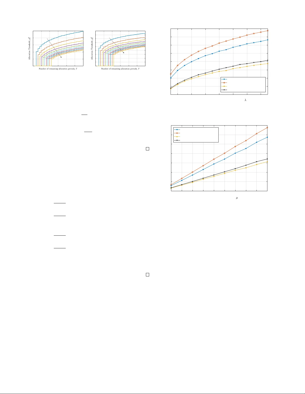
1 Dynamic Spatio-T emporal Resource Pro visioning for On-Demand Urban Services in Smart Cities Muhammad Junaid Farooq and Quan yan Zhu Department of Electrical & Computer Engineering, T andon School of Engineering, Ne w Y ork Uni versity , Brooklyn, NY 11201, USA, Emails: { mjf514, qz494 } @nyu.edu. Abstract —Efficient allocation of finite r esources is a crucial problem in a wide variety of on-demand smart city applications. Service requests often appear randomly over time and space with varying intensity . Resource provisioning decisions need to be made strategically in real-time, particularly when there is incomplete information about the time, location, and intensity of future requests. In this paper , we develop a systematic approach to the dynamic resource pro visioning problem at a centralized source node to spatio-temporal service requests. The spatial statistics are combined with dynamically optimal decision- making to derive recursive threshold based allocation policies. The developed results are easy to compute and implement in real-time applications. For illustrative purposes, we present ex- amples of commonly used utility functions, based on the power law decay and exponential decay coupled with exponentially , and uniformly distributed intensity of stochastic arrivals to demonstrate the efficacy of the developed framework. Semi- closed form expressions along with r ecursive computational procedur e has been provided. Simulation results demonstrate the effectiveness of the proposed policies in comparison with less strategic methodologies. Index T erms —Internet of things, smart cities, spatio-temporal Poisson process, r esource allocation. I . I N T R O D U C TI O N The integrated networks of engineered cyber and physical systems, referred to as the Internet of Things (IoT), provides the enabling technology for cities to greatly improve the se- curity , life, and wellbeing of its citizens [1]. The smart cities paradigm is creating a plethora of opportunities to efficiently utilize a vailable city resources 1 [2]. Resource allocation prob- lems occur in a wide variety of scenarios in smart cities such as in disaster management, emergenc y response systems, public safety systems, taxi pickups, controlling epidemic outbreaks, data collection using wireless sensors, etc. [3]. T ypically , there is a centralized sour ce node having a finite number of av ailable resources that need to be allocated to demand nodes or service r equests that arri ve sequentially o ver time at random locations with v arying sev erity or intensity . The task of the source node is to allocate av ailable resources to service requests in real-time to maximize the total e xpected utility 2 obtained from allocation. Fig. 1 illustrates a snapshot of the spatially disperse service requests that hav e accumulated ov er time with reference to a centralized source node placed at the origin serving a circular region. The height of impulses at the request locations 1 The term ‘resources’ may generically refer to emergency response units, taxis, wireless channels, aerial vehicles, vaccines, etc. 2 The term ‘utility’ used in the paper may refer to different quantities such as social welfare, revenue, etc., according to the application scenario. Fig. 1: Illustration of the centralized resource allocation problem during one time slot. The impulse height represents the intensity of requests. The maximum intensity request is highlighted by a bold blue impulse with an arrowhead. represents the intensity or magnitude of the demand. One of the potential ways to provision resources is to immediately allocate upon the arri val of a request re gardless of its intensity or distance. Howe ver , it may result in myopic decisions lead- ing to a suboptimal outcome. In man y practical applications, the decision is made once a pool of requests is available. The challenge in the allocation decision by the source is two-fold. Firstly , a very high intensity demand request may need service but it may be located at a farther distance from the source. Secondly , the source needs to decide whether to allocate a resource to one of the current requests or to wait for future requests, which may result in higher benefit. While discarding allocation to current requests, the source might keep waiting for better requests that never arriv e in the future. In essence, the question is where to draw the line for allocation in terms of distance and intensity of request as well as the waiting time of allocation. As an example, consider a data collection problem where a centralized base station (BS) schedules the uplink transmis- sion of spatially deployed sensor nodes. The sensor nodes randomly request for data collection to the BS informing it about their location as well as the channel state information 3 . The base station then decides whether to collect data from the sensor or to discard it. If the sensor is close to the BS but the channel gain is extremely lo w , then the probability of suc- cessfully obtaining data from it might be low . Howe ver , if the sensor is located far away but the channel gain is extremely high, there might be a strong chance of successfully retrie ving data from it. Therefore, the BS needs to optimally select the nodes, from which to collect data, considering the limited number of time slots that are av ailable to obtain data. Note 3 W e assume that sensor nodes are always able to communicate low bandwidth signaling information to the BS via separate control channels. that both the spatial and temporal components are highly important in the decision making while allocating decisions. A. Related W ork T raditionally , resource allocation problems have been well studied in the Operations Research literature and are re- ferred to as assignment problems. The classical bipartite assignment problem can be solved using the frame work of Optimal T ransportation [4], which is efficiently com- puted using Linear Programming for certain utility functions. Similarly , methods to solve the combinatorial optimization problems entailing to the assignment problem are av ailable such as the Hungarian algorithm [5]. Modified versions of these methods in volving con ve x optimization hav e been dev eloped to solve resource allocation problems in several applications, e.g., radio resource management in wireless communications [6], taxi dispatch [7], data collection [8], etc. Howe ver , these techniques only present static and off- line solutions that cannot be implemented in real-time when there is incomplete information about future arriv als. Those that consider stochastic arriv als do not take the spatial aspect into account [9]. Recent works that attempt to tackle spatio-temporal re- source provisioning problems in smart city applications in- clude mobile data upload planning [10], cloud/fog comput- ing resource allocation to applications [3], communication resource management for network operators [11], urban sensing [12], and socially responsible resource distribution in smart cities [1]. Howe ver , these works mainly use static assignment and are based on heuristic approaches to optimize the resource provisioning problem. Those that use arriv al dynamics, e.g., in a crowd sensing application [13], make use of queueing models, in which the unserviced requests remain in the system. The realtime allocation of resources to stochastic incoming requests has been dev eloped in [14]. Howe ver , there is no waiting time in volved and an allocation decision is made immediately upon arriv al of requests. In practical applications, the decision making process may not be immediate. Hence, the source node may wait for an allocation period and decide to allocate a resource that may lead to the maximum benefit. In general, there is a lack of systematic and prov ably optimal approaches for centralized resource allocation to spatio-temporal service requests. B. Contributions In this work, we attempt to combine the spatio-temporal aspect along with incomplete information about resource requests to devise an integrated resource provisioning frame- work. W e lev erage ideas from the seminal work on stochastic assignment of sequentially arriving tasks to workers [9]. Howe ver , the model has been enriched to encompass a more generic utility function that also incorporates the spatial dimension of the sequentially arriving requests. W e make use of spatial point processes in conjunction with order statistics and dynamic programming to dev elop an integrated and holistic policy framework that can act as the foundation for allocation and pricing in a wide v ariety of applications in the context of smart city applications. The rest of the paper is org anized as follows: Section II presents an elaboration of the system model and problem description, Section III provides details on the solution methodology , Section IV contains numerical and simulation results, while Section V concludes the paper with insights on future research directions. I I . S Y S T E M M O D E L Consider a typical source node at the origin with a discrete number of identical resources denoted by N ∈ Z + . The source is assumed to hav e an omni-directional service range of R ∈ R + . Service requests dynamically appear inside the served region according to a spatio-temporal Poisson Process with intensity λ ( r , θ , t ) : [0 , R ] × [0 , 2 π ] × R + → R + , where the pair ( r , θ ) represent the Polar coordinates of the service requests. Each service request is characterized by the tuple ( X i , D i ), where X i ∈ R + denotes the intensity of the request and D i ∈ [0 , R ] denotes its distance from the source node. It is assumed that both the distance and the intensity of requests is known at the source. Further , we assume that once a resource is allocated to service request, it becomes unav ailable for allocation in the future. A. Characterization of Service Requests W e assume a time slotted system with t = [1 , 2 , . . . , T − 1 , T ] , where each time slot of duration τ represents an allocation period, also referred to as the decision horizon. T o avoid non-uniformity in the av erage number of requests within allocation periods, we assume that the requests are uniform in the temporal domain, i.e., λ ( r, θ , t ) = τ ˜ λ ( r , θ ) , where τ ∈ R + is a constant. Note that this assumption is not restricti ve, since otherwise the width of time slots can be adjusted to create a uniform temporal profile of requests. In each time slot, the service requests are distrib uted spatially according to a Poisson Point Process (PPP). It implies that the number of requests in a circle of radius R during one allocation period, denoted by K follows a Poisson distribution with av erage density Λ . The probability density function (pdf) of K can be expressed as follows: P ( K = k ) = e − Λ (Λ) k k ! , (1) where the, average density of service requests during each allocation period, can be ev aluated as follows: Λ = E [ K ] = Z 2 π 0 Z R 0 τ ˜ λ ( r , θ ) r d r d θ. (2) Each service request has a type that represents the severity , criticality , or magnitude of demand. W e model it as inde- pendent and identically distributed (i.i.d.) random variables X i , i ∈ { 1 , . . . , K } , for each allocation period. Furthermore, we assume that the pdf, denoted by f X ( x ) , and cumulative distribution function (cdf), denoted by F X ( x ) , of the intensity is known at the source 4 . In order to exclude trivial cases in the resource allocation problem, we exclude the possibility of having no service request during an allocation period. It is stated formally stated as follows. 4 In practical situations, the statistical information about service requests can be obtained using spatio-temporal estimation techniques [15]. Assumption 1. W e assume that there is at least one service r equest in every allocation period. Therefor e we use the zero- truncated P oisson distribution to characterize the pdf of the number of service requests as follows: P ( K = k | K > 0) = e − Λ (Λ) k (1 − e − Λ ) k ! . (3) From the perspecti ve of the source node, the distance of each service requests during an allocation period is also a random variable, which is independent of the intensity . The probability distribution of the distances can be expressed by the following lemma. Lemma 1. The pdf of the distance D , of a randomly selected service r equest inside a cir cular r egion of radius R fr om the sour ce node, can be expr essed as follows: f D ( d ) = R 2 π 0 d ˜ λ ( d, θ )d θ R 2 π 0 R R 0 ˜ λ ( r , θ ) r d r d θ . (4) Pr oof. See Appendix A . B. Utility of Resource Allocation W e assume a generic utility function that characterizes the benefit obtained by allocating a resource to a service request of intensity X i that is located at a distance of D i from the source. The utility is denoted by U ( X i , D i ) : R + × [0 , R ] → R + . The utility function is assumed to be monotonically increasing in X i and monotonically decreasing in D i 5 , since allocating a resource at a higher distance may incur additional cost. If the utility of obtained by allocating a resource to each service request during a single time slot is denoted by Z i = U ( X i , D i ) , then Z i is also a random variable with the i.i.d. property formally expressed in the following remark. Remark 1. The random variables Z i = U ( X i , D i ) , i = 1 , . . . , K , ar e i.i.d. random variables since X i and D i ar e i.i.d., respectively . For notational conv enience, we will henceforth drop the index i and refer to the random variables describing the utility as Z . The cdf and pdf of the random variable Z can be ev aluated as follows: Lemma 2. The cdf and pdf of the random variable Z describing the utility of allocation to a randomly selected service request can be evaluated, r espectively as follows: F Z ( z ) = P [ Z ≤ z ] = Z Z S f X ( x ) f D ( d )d x d d, (5) and f Z ( z ) = d dz Z Z S f X ( x ) f D ( d )d x d d, (6) wher e S = { ( x, d ) : U ( x, d ) ≤ z } . W e define the maximum utility during each time slot j ∈ { 1 , . . . , T } as follo ws: ˜ Z j = max 1 ≤ i ≤ K j Z i , (7) 5 It implies that the utility is higher for close and high intensity requests and vice versa. where K j , j = 1 , . . . , T are i.i.d. Poisson random v ariables with mean Λ . Since the random variables ˜ Z j , j ∈ { 1 , . . . , T } , for all time slots are also i.i.d, we hereby drop the subscript and refer to it as ˜ Z . Then using extreme v alue theory , the pdf of ˜ Z can be expressed by the following lemma: Lemma 3. The pdf of ˜ Z = max { Z 1 , Z 2 , . . . , Z K } , where { Z i } 1 ≤ i ≤ K ar e i.i.d. random variables with cdf F Z ( z ) and pdf f Z ( z ) , and K is a P oisson random variable with mean Λ , can be expr essed as follows: f ˜ Z ( z ) = Λ f Z ( z ) e Λ( F Z ( z ) − 1) 1 − e − Λ . (8) Pr oof. See Appendix B . C. Pr oblem Definition The source has a total of T allocation periods during which it needs to allocate all the N ≤ T av ailable resources to incoming requests. Instead of delaying allocation decision until all the requests hav e appeared, the goal is to decide allocation in real-time. Therefore, a mechanism is required to allocate resources dynamically while maximizing the total expected utility obtained from allocation. During each allo- cation period, the decision problem is whether to allocated a resource to one of the current utility maximizing requests or to wait for the next batch of requests to decide. The resource provisioning problem can be formally ex- pressed as follows: max { i 1 ,i 2 ,...,i T }∈ ξ T X j =1 E [ ˜ Z j q i j ] (9) where ξ is the set of all possible permutations of the integers 1 , . . . , T and the vector q = [ q 1 , q 2 , . . . , q T ] is such that q 1 = q 2 = . . . = q N = 1 and q N +1 = q N +2 = . . . = q T = 0 . The objectiv e of the optimization is to find the permutation vector [ i 1 , i 2 , . . . , i T ] that maximizes the total expected utility . I I I . O P T I M A L D Y N A M I C A L L O C A T I O N M E C H A N I S M In this section, we describe the process to solve the optimization problem expressed in (9). Howe ver , we would first like to emphasize the fact that the decision problem is only relev ant if N ≤ T , i.e., the number of av ailable resources are less than the number of allocation periods. In other words, if the number of resources is more than the number of allocation periods, then the optimal policy would be to allocate a resource to the utility maximizing request in every allocation period. A grid representing the possible pairs of ( T , N ) is illustrated in Fig. 2. A. Optimization W e denote the optimal value obtained by solving the optimization problem in (9) if T allocation periods are remaining and N resources are av ailable as V ( T , N ) . Let ρ N T ∈ R + denote the decision threshold on the random variable ˜ Z if T allocation periods are remaining and N resources are av ailable. Then, the value function can be expressed recursiv ely using the following lemma: Lemma 4. If T allocation periods ar e r emaining and N r esour ces are available, then the total value obtained, in 1 2 3 4 5 0 1 2 3 4 5 4 5 N T Fig. 2: Red dots indicate the boundary cases for the pair ( T , N ). Blue dots indicate the cases for which the decision problem needs to be solved for allocation. the case when a r esource is allocated to the r equest and in the case when the request is discar ded can be expr essed as follows: V ( T , N ) =  ˜ Z T + E [ V ( T − 1 , N − 1)] , if ˜ Z ≥ ρ n T , E [ V ( T − 1 , N )] , if ˜ Z < ρ n T . (10) Pr oof. See Appendix C . Using this value function, the optimal allocation thresholds can be obtained using the procedure provided in the follo wing theorem. Theorem 1. If ther e ar e T allocation periods and N homo- geneous resour ces available, then it is optimal to allocate an available resour ce to a utility maximizing r equest, character - ized by ˜ Z T , i.e., q T = 1 , if ˜ Z T ≥ ρ n T , (11) wher e the thresholds ρ n T can be obtained as ρ n T = E [ V ( T − 1 , n )] − E [ V ( T − 1 , n − 1)] , (12) and the expected value functions with T allocation periods and N r esour ces can be computed recur sively as follows: E [ V ( T , n )] = Z ∞ ρ n T  ˜ Z + E [ V ( T − 1 , n − 1)]  f ˜ Z ( z ) dz + E [ V ( T − 1 , n )] F ˜ Z ( ρ n T ) . (13) Pr oof. See Appendix D . T o complete the optimal recursive solution, we need to ev aluate the boundary conditions, i.e., the expected v alue functions for the ( T , N ) pairs highlighted by the red dots in Fig. 2. The expected values for such cases can be expressed by the following lemma. Lemma 5. The expected value obtained for the boundary cases of ( T , N ) can be evaluated as follows. E [ V ( T , 0)] = 0 , (14) E [ V ( n, n )] = n E [ ˜ Z ] . (15) Pr oof. It follows from Theorem 1 that ρ n n = E [ V ( n − 1 , n )] − E [ V ( n − 1 , n − 1)] = 0 , ∀ n ∈ Z + . It means that if the number of allocation periods equal the number of av ailable resources, then the resource should be allocated to the utility maximizing request during that period regardless of the utility . Using this fact and the definition of V ( T , N ) , the result for E [ V ( n, n )] can be proved inductiv ely . B. Computation & Implementation In this section, we explain the procedure to compute the optimal allocation thresholds and provide an overvie w on implementing the proposed framework. In the case where there is one resource and two remaining time slots, the value function can be written as follows: V ( T = 2 , N = 1) =  ˜ Z if ˜ Z ≥ ρ 1 2 , ρ 1 2 if ˜ Z < ρ 1 2 . (16) where the threshold ρ 1 2 = E [ V (1 , 1)] = E [ ˜ Z ] . In the case that there is one resource and T = 3 time slots remaining, then the value function can be expressed as follows: V ( T = 3 , N = 1) =  ˜ Z if ˜ Z ≥ ρ 1 3 , E [ V (2 , 1)] if ˜ Z < ρ 1 3 , (17) where ρ 1 3 = E [ V (2 , 1)] − E [ V (2 , 0)] = R ∞ ρ 1 2 z f ˜ Z ( z ) dz + ρ 1 2 F ˜ Z ( ρ 1 2 ) . Howe ver , ρ 1 2 is av ailable from the previous step. Similarly , by computing E [ V (3 , 1)] enables the computation of ρ 2 3 and V (3 , 2) . This process needs to be executed re- cursiv ely to obtain the value functions and the thresholds for arbitrary number of allocation periods and a vailable resources. The step-wise procedure for computing the alloca- tion thresholds is summarized in Algorithm 1 and a summary of the implementation procedure is provided in Algorithm 2. Once, the form of U ( X , D ) is known, the optimal thresholds ρ N T translate to concentric surfaces, as shown in Fig. 3, that can be used to compare the maximal utilities in each time slot based on the number of av ailable resources and time slots remaining to decide on allocation. I V . R E S U LTS & D I S C U S S I O N In this section, we first present some special cases for which the optimal solution can be obtained numerically . Then we provide simulation results to demonstrate the practical implementation and effecti veness of the proposed framew ork. For sake of simple presentation of results, we assume a homogeneous spatio-temporal intensity of service requests, i.e., λ ( r, θ , t ) = τ λ . Then, service requests are distributed according to a Poisson process with intensity Λ = R 2 π 0 R R 0 λτ r d r d θ = τ λπ R 2 . For analytical tractability and practical relev ance, we will use two specific form of utility functions, i.e., U ( X , D ) = X (1 + D ) − η , η ≥ 0 , Fig. 3: Spatial requests in one allocation period. The bold arrow represents the request with maximum intensity . Con- centric surfaces correspond to the allocation thresholds if one, two, and three resources are available respectiv ely . Algorithm 1 Optimal Threshold Computation 1: procedur e T H R E S H O L D C O M P U T A T I O N Require: F Z ( z ) , f Z ( z ) , E [ ˜ Z ] . 2: Initialize: E V ← [ 0 T × N ] , ρ ← [ 0 T × N ] . 3: for i = 1 to T do 4: for j = 1 to N do 5: if i = j then 6: E V ( i, j ) ← j × E [ ˜ Z ] . 7: end if 8: end f or 9: end f or 10: for i = 1 to T do 11: for j = 1 to N do 12: if j = 1 then 13: ρ ( i, j ) ← E V ( i − 1 , j ) . 14: E V ( i, j ) = R ∞ ρ ( i,j ) ˜ Z f ˜ Z ( z ) dz + E V ( i − 1 , j ) F ˜ Z ( ρ ( i, j )) . 15: else 16: ρ ( i, j ) ← E V ( i − 1 , j ) − E V ( i − 1 , j − 1) . 17: Compute E V ( i, j ) using (13). 18: end if 19: end f or 20: end f or 21: end procedur e referred to as the power law utility 6 and U ( X , D ) = X e − αD , referred to as the exponential utility . A. Special Cases 1) P ower Law Utility: In this section, we assume that the utility function is of the form of U ( X , D ) = X (1 + D ) − η , η ≥ 0 . W e will further break do wn into two special cases, i.e., when the intensities of requests are exponentially and uniformly distributed. Case I: Exponential Intensity If X ∼ Exp ( µ − 1 ) , then F X ( x ) = 1 − e − µx , x ≥ 0 , and f X ( x ) = µe − µx , x ≥ 0 , then the pdf and cdf of the utility of each service request can be expressed by the following corollary . Corollary 1. The pdf and cdf of the utility Z of a service r equest inside a cir cular r e gion of radius R if U ( X , D ) = X (1 + D ) − η and X ∼ Exp( µ − 1 ) , can be evaluated as follows: F Z ( z ) = 1 − 2 η R 2  E η − 2 η ( z µ ) − (1 + R ) 2 E η − 2 η ( z µ (1 + R ) η ) − E η − 1 η ( z µ ) + (1 + R ) E η − 1 η ( z µ (1 + R ) η )  , (18) wher e E n ( x ) = R ∞ 1 e − xt t η dt is the generalized exponential inte gral. f Z ( z ) = Z R 0 µd (1 + d ) η e − µz (1+ d ) η d d. (19) Pr oof. See Appendix E . 6 Power law models are commonly used to model the propagation of wireless signals. Algorithm 2 Spatio-temporal Resource Allocation 1: procedur e R U NT I M E Require: T , N , ρ . 2: while T ≥ 0 do 3: Obtain the tuple ( X i , D i ) 1 ≤ i ≤ K . 4: Compute the utility U ( X i , D i ) for all requests. 5: Determine the maximal utility ˜ Z using (7). 6: if ˜ Z ≥ ρ ( T , N ) then 7: Allocate a resource to request corresponding to ˜ Z . 8: N ← N − 1 9: else 10: Skip allocation in the current allocation period. 11: end if 12: T ← T − 1 13: end while 14: end procedur e Case II: Uniform Intensity If X ∼ Unif (0 , β ) , then F X ( x ) = x β , x ∈ (0 , β ) and f X ( x ) = 1 β , x ∈ (0 , β ) , then the pdf and cdf of the utility of each service request can be expressed by the following corollary . Corollary 2. The pdf and cdf of the utility Z of a service r equest inside a cir cular r e gion of radius R if U ( X , D ) = X (1 + D ) − η and X ∼ U(0 , β ) , can be evaluated as follows: F Z ( z ) =                            2 z β R 2 1+  ( β z ) 1 /η  η +1 ( R ( η +1) − 1) 2+3 η + η 2 ! , if 0 ≤ z ≤ β (1 + R ) − η 2 z β R 2  1+( R +1) η +1 (( η +1)  ( β z ) (1 /η )  − η − 2) 2+3 η + η 2  + 2 R 2 R 2 2 − 1 2   β z  1 /η − 1  2 ! , if β (1 + R ) − η < z ≤ β and f Z ( z ) =                      2 β R 2  1+( R +1) η +1 ( R ( η +1) − 1) 2+3 η + η 2  , if 0 ≤ z ≤ β (1 + R ) − η 1 β R 2 η  2 η  1 − 2  β z  1+2 /η +  β z  η +1 η  − 4  β z  η +1 η   β z  1 /η − 1  , if β (1 + R ) − η < z ≤ β (20) Pr oof. See Appendix F . 2) Exponential Utility: In this section, we assume that the utility function is of the form of U ( X , D ) = X e − αD , α ≥ 0 . W e will further break down into two special cases, i.e., when the intensities of requests are exponentially and uniformly distributed. Case I: Exponential Intensity If the intensity of requests follows an exponential distribution with mean µ − 1 , then the pdf and cdf of the utility of each service request can be expressed by the following corollary . Corollary 3. The pdf and cdf of the utility Z of a service r equest inside a circular r egion of radius R if X e − αD , α ≥ 0 0 5 10 15 20 25 30 0 0.5 1 1.5 2 2.5 Power Law Utility with Exponential Intensity N = 1,2,...,10 (a) Power law utility with exponen- tial intensity . 0 5 10 15 20 25 30 0 0.5 1 1.5 2 2.5 3 3.5 4 4.5 Power Law Utility with Exponential Intensity N = 1,2,...,10 (b) Exponential utility with exponen- tial intensity . Fig. 4: Resource allocation thresholds for exponential inten- sity of service requests. and X ∼ Exp( µ − 1 ) , can be evaluated as follows: F Z ( z ) = 1 − 2 R 2 Z R 0 de − µz e αd d d. (21) and f Z ( z ) = Z R 0 2 µd R 2 e αd − µz e αd d d. (22) Pr oof. The proof follows a similar methodology as used in Appendix E and has been omitted for brevity . Case II: Uniform Intensity If the intensity of requests follo ws a uniform distribution in (0 , β ) , then the pdf and cdf of the utility of each service request can be expressed by the following corollary . Corollary 4. The pdf and cdf of the utility Z of a service r equest inside a circular r egion of radius R if X e − αD , α ≥ 0 and X ∼ U(0 , β ) , can be evaluated as follows: F Z ( z ) =        2 z α 2 β R 2  1 + e αR ( αR − 1)  , if 0 ≤ z ≤ β e − αR 2 α 2 β R 2  z + z e αR ( αR − 1)  , if β e − αR < z ≤ β (23) f Z ( z ) =        2 α 2 β R 2  1 + e αR ( αR − 1)  , if 0 ≤ z ≤ β e − αR 2 α 2 β R 2  1 + e αR ( αR − 1)  , if β e − αR < z ≤ β (24) Pr oof. The proof follows a similar methodology as used in Appendix F and has been omitted for brevity . B. P erformance Evaluation & Comparison T o illustrate the performance of our dev eloped resource provisioning framework, we conduct simulation experiments. The model parameters, unless otherwise stated, are selected as follo ws for illustrativ e purposes: service range R = 1 , service request density λ = 10 requests per unit area, duration of each time slot τ = 1, number of time slots T = 30 , number of a vailable resources N = 10 , mean of exponential intensity µ − 1 = 1 , parameter of uniform intensity β = 1 . Service requests are generated according to the homogeneous spatio-temporal Poisson process in a circular region around the origin. At each successiv e time slot, the maximum utility is pick ed and a resource is allocated 2 4 6 8 10 12 14 Intensity of spatio-temporal requests, 0 2 4 6 8 10 12 14 16 Total Expected Utility N = 10, T = 50 Optimal Allocation (Realtime) Ideal Allocation (Offline) Myopic Allocation Random Allocation Fig. 5: T otal expected utility against v arying spatio-temporal density of requests. 1 2 3 4 5 6 7 8 9 10 Mean intensity of requests, -1 0 2 4 6 8 10 12 14 Total Expected Utility N = 10, T = 50 Optimal Allocation (Realtime) Ideal Allocation (Offline) Myopic Allocation Random Allocation Fig. 6: T otal expected utility against varying intensity of requests. to the corresponding request only if the utility is higher than the threshold. Otherwise the requests are discarded and the next time slot is observed until the terminal time is reached. Fig. 4 plots the optimal allocation thresholds against the number of allocation periods remaining for dif ferent number of available resources at the source node if the intensity is assumed to be exponentially distributed. The threshold successiv ely increase as more allocation periods are av ail- able for the same number of av ailable resources. In other words, the source becomes more selective in allocation as more allocation periods are av ailable. Similarly , for a given number of allocation periods, the threshold decreases as the the number of av ailable resources increase. Note that the threshold remains zero if the number of av ailable resources and remaining allocation periods are equal. The successi ve difference between the thresholds is attributed to the fact that the intensity of requests is exponentially distributed. A similar behavior will be observed in the case of uniformly distributed arriv als except that the difference between suc- cessiv e thresholds is expected to be uniform. W e also compare our proposed resource provisioning framew ork with benchmark schemes namely the Ideal allo- cation, myopic allocation, and random allocation. The Ideal allocation represents the case when there is no uncertainty about the future and the maximum utilities in each time slot are known a priori. Therefore, it results in the best possible resource allocation strategy . The Myopic allocation strategy allocates a resource to the utility maximizing request in each time slot regardless of its magnitude. The random allocation is a generalization of the myopic allocation where in ev ery time slot, a resource is allocated to the utility max- imizing request with a probability of 0.5. If the probability of allocation is further reduced, there may be an increase in total expected utility since there is a higher chance of hitting better utility requests. Fig. 5 and Fig. 6 plot the total expected utility of allocation under v arying intensity of spatio-temporal requests and the mean intensity of requests respectiv ely . The simulation results clearly show that the proposed optimal allocation strategy lower expected utility as compared to the Ideal allocation. The loss in utility is due to the fact that allocation decisions are made in real- time without information about future arri val of requests. Howe ver , it performs at least two-fold better than the myopic and random allocation strategies. V . C O N C L U S I O N S & F U T U R E W O R K In this paper , we have proposed a utility maximizing approach to allocate resources from a centralized source location to spatio-temporal service requests with varying intensity . The framew ork is highly generic in terms of the utility of allocation, the number of a vailable resources and the number of allocation periods along with the spatio-temporal statistics of the requests. Using statistical analysis of the util- ity obtained by the allocation, we ha ve dev eloped an optimal filtering scheme that makes only qualifying requests eligible for resource allocation. The de veloped resource provisioning framew ork is en visioned to have wide ranging applications in smart cities. Sev eral useful extensions can be done to enhance the proposed frame work to cater for more realistic and tailored scenarios for different resource allocation problems. The cost of delaying the allocation can be added as a parameter to the framework to prev ent over -selectiv eness of the source. Furthermore, the case of non-homogeneous resources and the continuous time version of the framework can be in vestigated to cater for more versatile scenarios and applications. A P P E N D I X A P RO O F O F L E M M A 1 The cdf of the distance to a typical service request in a non-homogeneous PPP model with density τ ˜ λ ( r , θ ) can be ev aluated as follows: F D ( d ) = P ( D ≤ d ) = R 2 π 0 R d 0 ˜ λ ( r , θ ) r d r d θ R 2 π 0 R R 0 ˜ λ ( r , θ ) rdr dθ . The pdf can then be obtained as follo ws: f D ( d ) = d F D ( d ) d d = R 2 π 0 d ˜ λ ( d, θ )d θ R 2 π 0 R R 0 ˜ λ ( r , θ ) r d r d θ . In the special case of a homogeneous PPP , i.e., ˜ λ ( r , θ ) = τ λ , the cdf and pdf of the distance can be expressed as follo ws: F D ( d ) = P ( D ≤ d ) = τ λπ d 2 τ λπ R 2 = d 2 R 2 , (25) f D ( d ) = dF D ( d ) d d = 2 d R 2 . (26) A P P E N D I X B P RO O F O F L E M M A 3 The distribution function of ˜ Z = max { Z 1 , Z 2 , . . . , Z K } with K being a Poisson random variable can be obtained as follows: F ˜ Z ( z | K = k ) = P ( ˜ Z ≤ z | K = k ) , = P (max { Z 1 , Z 2 , . . . , Z K } ≤ z | K = k ) , = P ( Z 1 ≤ z , Z 2 ≤ z , . . . , Z K ≤ z | K = k ) , = K Y i =1 P ( Z i ≤ z ) = K Y i =1 F ˜ Z ( z ) = ( F Z ( z )) K . (27) Consequently , the conditional pdf of ˜ Z can be expressed as follows: f ˜ Z ( z | K = k ) = dF ˜ Z ( z | K = k ) dz = k ( F Z ( z )) k − 1 f Z ( z ) . (28) Finally , the pdf can be obtained as follo ws: f ˜ Z ( z ) = ∞ X k =1 f ˜ Z ( z | K = k ) P ( K = k | K > 0) , = ∞ X k =1 k ( F Z ( z )) k − 1 f Z ( z ) e − Λ (Λ) k (1 − e − Λ ) k ! , = Λ f Z ( z ) e Λ( F Z ( z ) − 1) 1 − e − Λ . (29) A P P E N D I X C P RO O F O F L E M M A 4 T o prov e the recursi ve value function, we make use of the decision tree sho wn in Fig. 7. At the current allocation period, if there are T allocation periods remaining with N av ailable resources, there are two possible decisions, i.e., to allocate a resource to the utility maximizing request or to postpone allocation to a future allocation period. The value V ( T , N ) ˜ Z E [ V ( T − 1 , N − 1)] 0 E [ V ( T − 1 , N )] Fig. 7: Decision tree at when T allocation periods are remaining and N resources are av ailable. function can be expressed as follows: V ( T , N ) = (30) max q T { ˜ Z q T + E [ V ( T − 1 , N − 1) , E [ V ( T − 1 , N )] } . It is clear that if q T = 1 and ˜ Z T is greater than some threshold ρ N T , then ˜ Z + E [ V ( T − 1 , N − 1)] ≥ E [ V ( T − 1 , N )] . Therefore, V ( T , N ) = ˜ Z + E [ V ( T − 1 , N − 1)] . Otherwise, if q T = 0 , then E [ V ( T − 1 , N )] > E [ V ( T − 1 , N − 1)] , which results in V ( T , N ) = E [ V ( T − 1 , N )] . D X X = z (1 + D ) η R z (a) Shaded region for power law utility and exponential intensity . D X X = z (1 + D ) η R β z (b) Shaded region for power law utility and uniform intensity . Fig. 8: The shaded region represents the region of integration S = { ( x, d ) : U ( x, d ) ≤ z } . A P P E N D I X D P RO O F O F T H E O R E M 1 From the decision tree shown in Fig. 7, the decision to allocate a resource to a qualifying request is only made if the utility obtained from the allocation is higher than the utility obtained from postponing the decision. It implies that ˜ Z + E [ V ( T − 1 , n − 1)] ≥ E [ V ( T − 1 , n )] . (31) This leads to the condition that ˜ Z ≥ E [ V ( T − 1 , n )] − E [ V ( T − 1 , n − 1)] = ρ N T . (32) The expectation of the value function can be obtained directly from the definition in (4) in terms of the allocation threshold ρ N T . A P P E N D I X E P RO O F O F C O RO L L A RY 1 The pdf of Z can be ev aluated as follows: F Z ( z ) = P [ Z ≤ z ] = P [ X (1 + D ) − η ≤ z ] , = P [ X ≤ z (1 + D ) η ] . (33) This probability can be obtained by integrating the joint density f X,D ( x, d ) over the shaded region S = { ( x, d ) : U ( x, d ) ≤ z } sho wn in Fig. 8a. Consequently , the cdf can be expressed as follows: F Z ( z ) = Z R 0 Z z (1+ d ) η 0 f X ( x ) f D ( d )d x d d, = Z R 0 Z z (1+ d ) η 0 µe − µx × 2 d R 2 d x d d. (34) Computing the integrals results in the expression provided in Corollary 1. Furthermore, differentiating F Z ( z ) w .r .t. z results in f Z ( z ) . A P P E N D I X F P RO O F O F C O RO L L A RY 2 The pdf of Z can be ev aluated as follows: F Z ( z ) = P [ Z ≤ z ] = P [ X (1 + D ) − η ≤ z ] , = P [ X ≤ z (1 + D ) η ] . (35) This probability can be obtained by integrating the joint density f X,D ( x, d ) over the shaded region S = { ( x, d ) : U ( x, d ) ≤ z } shown in Fig. 8b. F Z ( z ) =              R R 0 R z (1+ d ) η 0 1 β × 2 d R 2 d x d d, if z ≤ β (1 + R ) − η R ( β z ) 1 η − 1 0 R z (1+ d ) η 0 1 β × 2 d R 2 d x d d + R R ( β z ) 1 η − 1 R β 0 1 β × 2 d R 2 d x d d, if β (1 + R ) − η < z ≤ β (36) Computing the integrals leads to the result in Lemma 2. The density function of Z can then be ev aluated by differ - entiating F Z ( z ) w .r .t. z . R E F E R E N C E S [1] H.-R. D. Tsai, Y . Shoukry , M. K. Lee, and V . Raman, “T owards a so- cially responsible smart city: Dynamic resource allocation for smarter community service, ” in Pr oceedings of the 4th ACM International Confer ence on Systems for Ener gy-Efficient Built En vir onments , ser . BuildSys ’17. Ne w Y ork, NY , USA: ACM, 2017, pp. 13:1–13:4. [2] J. Santos, T . V anhove, M. Sebrechts, T . Dupont, W . Kerckhove, B. Braem, G. V . Seghbroeck, T . W auters, P . Leroux, S. Latre, B. V olck- aert, and F . D. Turck, “City of things: Enabling resource provisioning in smart cities, ” IEEE Communications Magazine , vol. 56, no. 7, pp. 177–183, July 2018. [3] J. Santos, T . W auters, B. V olckaert, and F . D. Turck, “Resource provisioning for IoT application services in smart cities, ” in 13th International Confer ence on Network and Service Management (CNSM 2017) , Nov 2017, pp. 1–9. [4] C. V illani, Optimal T ransport: Old and New , ser . Grundlehren der mathematischen Wissenschaften. Springer, Sep 2008. [5] H. W . Kuhn and B. Y aw , “The hungarian method for the assignment problem, ” Naval Res. Logist. Quart , pp. 83–97, 1955. [6] H. Ghazzai, M. J. Farooq, A. Alsharoa, E. Y aacoub, A. Kadri, and M. Alouini, “Green networking in cellular hetnets: A unified radio resource management framework with base station ON/OFF switch- ing, ” IEEE T ransactions on V ehicular T echnology , vol. 66, no. 7, pp. 5879–5893, Jul. 2017. [7] F . Miao, S. Han, S. Lin, Q. W ang, J. A. Stankovic, A. Hendawi, D. Zhang, T . He, and G. J. Pappas, “Data-driv en robust taxi dispatch under demand uncertainties, ” IEEE T ransactions on Contr ol Systems T echnology , vol. 27, no. 1, pp. 175–191, Jan. 2019. [8] I. Ali, A. Gani, I. Ahmedy , I. Y aqoob, S. Khan, and M. H. Anisi, “Data collection in smart communities using sensor cloud: Recent advances, taxonomy , and future research directions, ” IEEE Communications Magazine , vol. 56, no. 7, pp. 192–197, July 2018. [9] C. Derman, G. J. Lieberman, and S. M. Ross, “ A sequential stochastic assignment problem, ” Management Science , vol. 18, no. 7, pp. 349– 355, 1972. [10] Q. Zhu, M. Y . S. Uddin, Z. Qin, and N. V enkatasubramanian, “Upload planning for mobile data collection in smart community internet- of-things deployments, ” in IEEE International Confer ence on Smart Computing (SMARTCOMP 2016) , May 2016, pp. 1–8. [11] D. Sahinel, C. Akpolat, F . Sivrikaya, and S. Albayrak, “ An agent- based network resource management concept for smart city services, ” in 14th Annual Conference on Wir eless On-demand Network Systems and Services (WONS 2018) , Feb 2018, pp. 129–132. [12] Q. Zhu, M. Y . S. Uddin, N. V enkatasubramanian, and C. Hsu, “Spa- tiotemporal scheduling for crowd augmented urban sensing, ” in IEEE Confer ence on Computer Communications (INFOCOM 2018) , April 2018. [13] Y . Han, Y . Zhu, and J. Y u, “Utility-maximizing data collection in crowd sensing: An optimal scheduling approach, ” in 12th Annual IEEE International Conference on Sensing, Communication, and Networking (SECON 2015) , June 2015, pp. 345–353. [14] M. J. Farooq and Q. Zhu, “ Adaptive and resilient revenue maxi- mizing dynamic resource allocation and pricing for cloud-enabled IoT systems, ” in Annual American Contr ol Conference (A CC 2018) , Milwaukee, WI, USA, Jun. 2018. [15] A. Malik, R. Maciejewski, S. T owers, S. McCullough, and D. S. Ebert, “Proactive spatiotemporal resource allocation and predictive visual analytics for community policing and law enforcement, ” IEEE T ransactions on V isualization and Computer Graphics , vol. 20, no. 12, pp. 1863–1872, Dec. 2014.