Second Order Statistics Analysis and Comparison between Arithmetic and Geometric Average Fusion

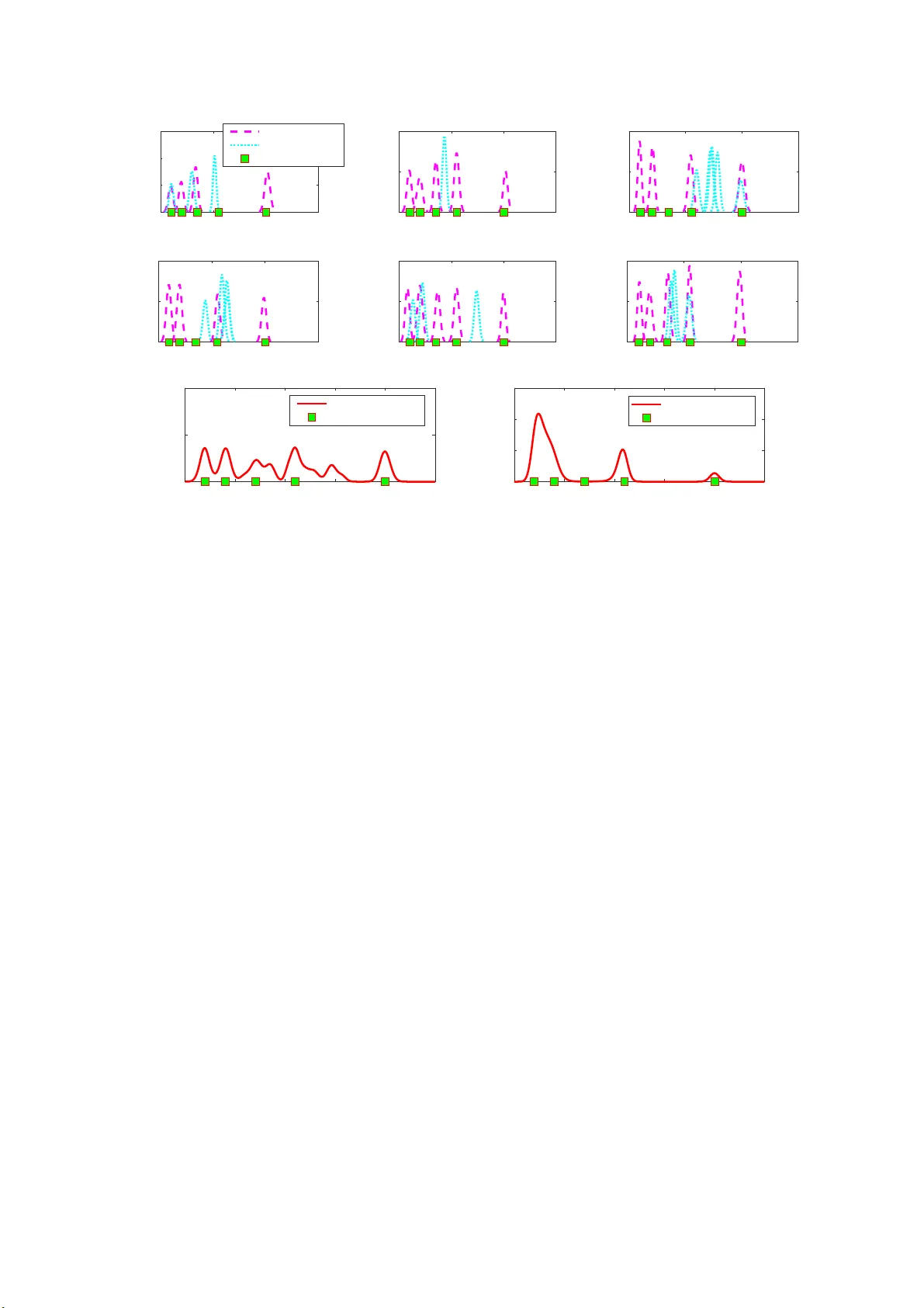
Second Order Statistics Analysis and Comparison between Arithmetic and Geometr ic A v era ge Fusion T iancheng Li* a,b,c , Hon gqi Fan d , Jes ´ us G. Herrero e , Juan M Corchado b,c,f a K e y Laborato ry of Informati on Fusion T ech nolo gy (Minist ry of Education), Scho ol of Automatio n, Northwestern P olytec hnica l Universit y , Xi’an 710072, China. E-mail: t.c.li@ { usal.es,mail.nwpu.edu.cn } b BISITE r esear ch Gr oup, Uni versi ty of Salamanca, Salamanca 37007, Spain c Air Instit ute , IoT Digital Inno vation Hub, Salamanca 37188 , Spain d National K e y Laboratory of Scienc e and T ec hnolo gy on ATR, Nat ional Univer sity of Defense T ec hnolo gy , Chang-Sha 410073, Chin a. E-mail:fanho ngqi@nudt .edu.cn e Department of Comput er Science and Engineeri ng, Universid ad Carlos III de Madrid, Calle Madrid 126, 28903 Getafe , Spain. E-mail:jghe rre r@inf .uc3m.es f Department of Electr onics, Information and Communication, Osaka Institute of T echnol ogy , Osaka 535-8585, Jap an Abstract T w o fundam ental approa c h es to infor mation averaging a r e ba sed on linear and logar ithmic com bination, y ielding the arithme tic av erage (AA) and geo metric average (GA) of the f using initials, respe c tively . In the co ntext o f target tracking, the two mo st co mmon form ats of data to be fused are rando m variables and probab ility density f unctions, namely v - fusion and f -fusion, respectively . In this work, we analy ze and compar e the second order statistics (includin g variance and mean square er ror) of AA and GA in te r ms of b o th v -fusion and f -fusion. The case o f weigh ted Gaussian mixtures representing multitarget densities in the presence of false alarms and misdetec tio n (wh ose weight sums are not n ecessarily unit) is also considered, the result of which a p pears significantly di ff erent from that for a single target. In add ition to exact d eriv ation , exemplifying analysis and illustra tions are pr ovid ed. K eywor d s: Multisensor fu sion, av erage consensus, distributed tracking , covariance in tersection, arithmetic mean , geometric mean, lin ear pool, log -linear p ool 1. Introduction The rapid development and extensive d eployment of senso r / agent ne twork s, have stemmed remark able inter est in distributed d ata f usion which demo nstrates evident a d vantages in many aspects. F or exam ple, in the context of target tr a cking using a decen tralized sen sor network, the sen so r c o operation can co mpensate for the e ff e ct of the mis- detection, false-alarms and even the failure of th e local sensor and extends their fields of view , ev entually resulting in improved estimation accuracy and improved robustness [1, 2, 3, 4 , 5, 6]. Particular interest in distributed data fusion has be en paid to calculatin g the “average” over th e info rmation owned b y locally n etted sen so rs / agents via p eer-to-peer commun ication in an e ffi cient, flexible and scalab le way [7, 8, 9, 6, 1 0]. Fundamen tally , the average can be defined in two manner s includ ing, the arithmetic average (AA) an d the geometric a verag e (GA). Simply put, the former is a type of linear / conve x fusion, akin to the line ar opinio n p ool app roach, while the latter is n onlinear / logarithmic f usion akin to th e logarithm ic opin ion pool appro ach [1 1, 12], or to say , linear versus log -linear pools [13]. In the context o f mu lti-sensor / multi-a g ent target tra c k ing, the two most impor tant types of infor mation for f u sion among local sensors / agen ts are rando m variables (re p resenting parameters su c h as the nu mber of targets, clu tter rate, target existing p robability , etc.) an d pr obability density functions (PDFs), for wh ich the fusion is referred to as v - fusion and f -fusion, respectively . While it seem s that the AA fusion is m o re c ommon in the form er [7, 8, 4 , 9], the GA fusion is vibrant in the latter [3, 14, 15], whic h coincides with the Chern o ff fusion [16, 17, 1 8, 19] and is also k nown as covariance inter sectio n (CI) when Gau ssian functio ns th at are uniqu ely ch a racterized by the first and second or der statistics are particu larly consider ed [2 0, 21, 22, 23, 24, 25]. The CI ap proach was origin ally propo sed for fusing unkn own-correlated estimates pro duced at distinct but not necessarily indep endent sensor s to av o id info rmation d ouble accounting in th e f usion. Likewise, the AA fusion can also av oid information double accountin g [2 2]. Further approach e s to com bining prob ability distributions of unk nown cross-co rrelation can be found in the literatur e [26, 2 7, 28, 29, 3 0]. In par ticular , a so-called generalize d mean fu sion ap proach is prop osed Prep rint submitted to Elsevi er J anuary 24, 2019 in [3 0] w h ich in cludes b oth AA a nd GA in a unified expression . It is interesting to n o te (fo r d iscr e te f -fusion ) that “ a linear o pinion poo l is the distribution that minimizes the sum of KL [Kullback - Leibler] mea sur es fr om the expert distributions to th e aggr e g ate distribution. A log-linear o p inion pool is one th at minimizes the sum of KL measures fr om the aggr egate distribution to the expert distributions. [13] ” This nice proper ty for the GA fusion was earlier pointed out in [11] and later extended to the PHD in [31]. In additio n to the p osterior PDF , th e fusing fu n ctions can also be the likelihoo d f unctions [32, 15, 33] or the probab ility h ypothesis d ensity (PHD) f u nctions [14, 34, 31, 35, 36, 37]. (The PHD [38] di ff ers from the PDF in that its integral over any region gives the expected n umber of targets in th at region which can b e any real n umber .) In comparison , th e AA fu sio n has also been applied for PHD fusion [ 39, 40, 4 1, 4 2, 43, 44, 45, 46] and for raw data fusion in the means o f clustering [ 47, 48]. Both averaging approach es to data fusion have demonstrated, either theoretically or experime n tally , g ains in estimation a ccuracy and / or robustness, wherea s d eficiencies h a ve also bee n identified from di ff e rent viewpoints [1 1, 12, 34, 49, 50, 41, 4 3, 44, 51, 52, 36, 3 0]. Despite a few analysis ab out the variance alone [21, 22, 14, 49] in f -fusion, th e mean squar e err o r (MSE) of the A A [45] in v -fusion an d the diver gence to the ideal fusion ru le in f -fusion [30], compreh ensiv e analysis and com parison of their statistics (in cluding the variance and MSE) are still lacking. What is missing an d interesting also in cludes the specific consider ation o f the multitarget density fu sio n in the p resence of false alar ms and misde tection. In this paper, we ar e not intende d to in vestigate th e motiv ation behind both ap proaches, or propose any new alg o - rithms. Rath er , we analy ze and compare the statistics of the GA and of the AA in the viewpoint of point estimation, with respe c t to v -fu sion and f -fusion, respectiv ely . In addition to a detailed forma l analysis, some approxim ations an d exemplifying illustrations are also given. Furth er , we restrict ou r discussion in the scala r real space R for simplicity , although most of the conclusio n s can be extended to th e multidimension a l case. The pape r is organ ized as f o llows. Preliminaries are briefly intr oduced in Section 2. Our major an alysis o f the v -fusion and of the f -fusion is given in sections 3 and 4, respectively . A hybrid u se of bo th approach es for a veraging PHDs is discussed in Sec tio n 5, as well as fur ther comp a r ison between v -fusion an d f -fusion . K ey find ings are summarized by Rem a rks through out the main body of the paper and in Section 6. 2. Preliminaries 2.1. Definitio n s For the u nknown par a m eter θ of interest that takes value in a m easurable region × ⊆ R , the estimator ˆ θ i associated with PDF f ˆ θ i ( x ) , is un b iased if it yield s, on average, the true value of the p arameter [53, Section 2.3], i.e., ¯ θ i , E f ˆ θ i [ ˆ θ i ] = Z × x f ˆ θ i ( x ) d x = θ . (1) The variance of the estimator ˆ θ i is given by Σ ˆ θ i , Z ×  x − ¯ θ i  2 f ˆ θ i ( x ) d x = Z × x 2 f ˆ θ i ( x ) d x −  ¯ θ i  2 . (2) The MSE o f an estimator ˆ θ i is given by [53, Section 2. 4] mse( ˆ θ i ) , E f ˆ θ i ( x ) [( θ − ˆ θ i ) 2 ] = Z × ( θ − x ) 2 f ˆ θ i ( x ) d x . (3) A straigh tforward expa n sion of (3) will lead to mse( ˆ θ i ) = Σ ˆ θ i + ( ¯ θ i − θ ) 2 . (4) That is, the MSE of an estimator equals th e sum of its variance an d the squa r e o f its bias (if any). Furthermo re, suppo se that f : X → R is a real- valued fu nction whose domain is a set X . The set-theor etic suppo rt of f , deno ted as supp( f ), is the set of po ints in X wh ere f is non-zer o, i.e., supp( f ) = { x ∈ X | f ( x ) , 0 } . (5) 2 2.2. A veraging in T erms o f V ariables: v-fusio n Let us c o nsider estimators ˆ θ i , i ∈ I ⊆ N given in term s of rand om variables, such as the estimate o f the nu mber of targets [45] o r the target existing probab ility . Ther e is n o PDF or uncertainty information available a n d so on ly point estimates that a r e rando m variables are inv olved. The variable-AA is given by ˆ θ AA v , X i ∈I ω i ˆ θ i . (6) Hereafter, the fusing weig hts are limited as ω i ∈ (0 , 1), P i ∈I ω i = 1. (Obvio u sly , ω i = 0 ind icates that informatio n i does not really get in volved in the fusion.) In con trast to (6), the variable-GA is g i ven b y ˆ θ GA v , Y i ∈I ˆ θ ω i i . (7) Note that, the variable-GA fu sio n may lead to an imagin ary n umber when th e fusing variable is negative, which is beyond the consider ation o f this work. Obviously , the GA fu sion amounts to the AA fusion on the log arithms of the variables, n amely (cf. (6)) log ˆ θ GA v = X i ∈I ω i log ˆ θ i . (8) 2.3. A veraging in T erms o f PDFs: f-fusion When the local e stima to r is g i ven as a function such as a PDF or a PHD, the f -fusion is in volved. Given estimators ˆ θ i with PDFs f ˆ θ i ( x ) , i ∈ I , th e PDF-AA is g i ven b y f ˆ θ AA ( x ) = X i ∈I ω i f ˆ θ i ( x ) , (9) and the PDF-GA is given by f ˆ θ GA ( x ) = C − 1 Y i ∈I  f ˆ θ i ( x )  ω i , (10) where C , R × Q i ∈I  f ˆ θ i ( x )  ω i d x is a nor malization term to ensure the re sult being a PDF (if p ossible). (In the gen eral- ized GA fusion a p plied to the PHDs [14, 34], such a n ormalization may be un necessary . But then, the fused result of two PDFs may n ot be a PDF [34]. ) Fundamen tally , the suppor t of the AA fusion PDF is the union of those of all initial PDFs. In con tr ast, th e sup p ort of f ˆ θ GA ( x ) is the in tersection o f those of all initial PDFs, which ma y be empty . W e leave here further d iscussion on this point and we assume all fu sing estimators have th e same supp ort unless otherwise stated. 3. Statistics Analysis for v -Fusion 3.1. Bias An a lysis Consider un biased estimators ˆ θ i , i ∈ I given as random variables. Th e unbiased ness indicates (c f. (1)) ¯ θ i = θ, ∀ i ∈ I . (11) Combining (6) a n d (11) y ields ¯ θ AA v = X i ∈I ω i ¯ θ i = θ . (12) That is, the AA retains the unbiasedn ess (namely it remains unb iased if all fu sing initials are u n biased.) Howe ver, as add ressed the variable GA fu sion may lea d to an imagin a ry result if a ny ˆ θ i is an imaginar y nu mber and so we c a nnot co mpare it with the AA mean in general. Even in the case that ˆ θ i , ∀ i ∈ I are all positiv e, the inequality of arithmetic and geometric mea n s [54, Chap ter 2] in dicates ¯ θ GA v ≤ ¯ θ AA v . Here, th e two mean s are equa l if and only if θ i = θ j , ∀ i , j ∈ I . I n a nutshe ll, the AA but not th e GA retains u nbiasedn ess in general. 3 3.2. V ariance Analysis The variance o f a weighted sum of mu ltiple variables is given by the weighted sum of their covariances, [55], i.e., Σ ˆ θ AA v = X i ∈I X j ∈I Cov( ω i ˆ θ i , ω j ˆ θ j ) = X i ∈I ω 2 i Σ ˆ θ i + X i < j ∈I 2 ω i ω j Cov( ˆ θ i , ˆ θ j ) . (13) Here, Cov( ˆ θ 1 , ˆ θ 2 ) d e n otes the covariance between ˆ θ 1 and ˆ θ 2 . Let us c o nsider two variables for simplicity and define the co rrelation coe ffi cient [56, Chapt. 4 ] as ρ , Cov( ˆ θ 1 , ˆ θ 2 ) p Σ ˆ θ 1 Σ ˆ θ 2 , (14) taking values between − 1 and 1 . (For two in depende nt variables, ρ = 0 an d for two identical variables, ρ = 1.) Then , (13) redu ces to Σ ˆ θ AA v = ω 2 1 Σ ˆ θ 1 + ω 2 2 Σ ˆ θ 2 + 2 ω 1 ω 2 ρ q Σ ˆ θ 1 Σ ˆ θ 2 . (15) W e now a n alyze th e bou nds of Σ ˆ θ AA v . First, it is easy to verify that Σ ˆ θ AA v ≤  ω 1 √ Σ 1 + ω 2 √ Σ 2  2 ≤ max( Σ 1 , Σ 2 ), indicating that Σ ˆ θ AA v ≤ max( Σ 1 , Σ 2 ) , (16) where the upper bound is a p proach e d w h en w 1 → 0 (if Σ 1 ≤ Σ 2 ) or w 1 → 1 (if Σ 1 ≥ Σ 2 ). T o derive th e lo wer b ound of Σ ˆ θ AA v , we f urther define α , Σ 2 Σ 1 . (17) Due to the sym metry of the expression o f Σ ˆ θ AA v , we on ly need to consider α ≥ 1 in o u r analysis; the results hold b y exchanging Σ 2 with Σ 1 if α < 1. Ou r analysis is based on a conv ex function of w ∈ (0 , 1) as fo llows h ( w ; α, ρ ) , 1 − 2 w + w 2 + w 2 α + 2 ρα 1 2 ( w − w 2 ) . (18) Bound an alysis of the fun ction h ( w ; α, ρ ) is giv en in Appendix A. Here after , we write h ( w ; α, ρ ) as h ( w ) fo r short. So, we have Σ ˆ θ AA v = h ( ω 2 ) Σ 1 . If ρ < α − 1 2 , the fusing weights that minimize h ( w ) are gi ven b y (cf. ( 55)) ω 1 = α − ρα 1 2 1 + α − 2 ρα 1 2 , ω 2 = 1 − ρα 1 2 1 + α − 2 ρα 1 2 . (19) This corre sp onds to the lower bound of Σ ˆ θ AA v as 1 Σ ˆ θ AA v ≥ α (1 − ρ 2 ) 1 + α − 2 ρα 1 2 Σ 1 . (20) Otherwise (if ρ ≥ α − 1 2 ), th e lower bou nd is given by Σ ˆ θ AA v ≥ min( Σ 1 , Σ 2 ) , (21) where the bo und is app roached wh en w 1 → 1 ( if Σ 1 ≤ Σ 2 ) or w 1 → 0 (if Σ 1 ≥ Σ 2 ). Remark 1 . F or v-fu sio n , the variance of the A A is up per boun d ed by the greatest variance of the fu sing estimato rs. Its lower bound as given in (20) is smaller tha n the smallest variance o f the fusing estimators if the corr elatio n coe ffi cient between two fusing estimator sa tisfie s Cov( ˆ θ 1 , ˆ θ 2 ) p Σ ˆ θ 1 Σ ˆ θ 2 <  min  Σ 1 , Σ 2  max  Σ 1 , Σ 2   1 2 , (22) otherwise, the lower bo und is giv e n b y the smallest variance of th e fusing estimators. 1 In the case of ρ = 0, the two fusing weights as in (19) are giv en by the inv erse of the opposite v arianc e di vided by the sum of the two in ve rses. The optimal fusion reduces to the classical Millman’ s equatio n [57], analogou s to the weighted least squares fusion of two indepen dent estimators. 4 0 0.2 0.4 0.6 0.8 1 w 1 0 50 100 150 200 250 = -0.7085 0 0.2 0.4 0.6 0.8 1 w 1 50 100 150 200 = 0.20885 0 0.2 0.4 0.6 0.8 1 w 1 100 120 140 160 180 200 = 0.70886 1 2 AA variance GA variance Figure 1: V arianc es of the AA and GA of two correlated, approximate- Gaussian-di stributed v ariabl es with mean µ 1 = 50 and vari ance Σ 1 = 100, and with mean µ 2 = 60 and vari ance Σ 2 = 200, respecti vely , under three di ff erent correla tion coe ffi ci ent ρ s . Notably , when these two variables are in versely correlated (n amely Cov( ˆ θ 1 , ˆ θ 2 ) < 0), (2 2) always holds. On the other hand , to calculate Σ ˆ θ GA v , substituting ˆ θ AA v , ˆ θ i , i ∈ I in (13) with log ˆ θ GA v , lo g ˆ θ i , i ∈ I (cf. (8)), respec tively , yields Σ log ˆ θ GA v = X i ∈I X j ∈I Cov( ω i log ˆ θ i , ω j log ˆ θ j ) = X i ∈I X j ∈I ω i ω j Cov(log ˆ θ i , lo g ˆ θ j ) . (23) The above for mulation in volves th e calculation of the covariance b etween (logar ithmic) functio ns of two ran dom variables, wh ich can be addressed in terms of the cumulative distribution fun ction; see, e.g., [58]. W e omit furth e r analysis o n this mathem atical problem , but instead, to gain insight an d to illustratively compare b etween the AA and the GA, we study two repr esentativ e examples by m e ans of the Monte Carlo simulatio n. 3.2.1. Numerical an alysis for Gau ssian v- fusion Note that the GA of two Gaussian variables is no longer a G a ussian variable ( u nless two fusing variables are identical). For numerical illustration , we here con sider two app roximate Gaussian distributions with µ 1 = 50 , Σ 1 = 100, and with µ 2 = 60 , Σ 2 = 20 0 , resp ecti vely , in which the negative su pport o f the Gaussian PDF (which is ac tually ignorab le in the g iven examples as the negative part is far mo re than four-sigma to the mean o f the distribution) is truncated and so all samples ar e guaran teed to be positively valued in order to avoid the imaginar y nu mber problem of the GA fusion. T wo gro ups of samples are gener ated with d i ff erent corr e lation co e ffi cient ρ s. Th e correspo n ding values of the mean and variance of the AA and of the GA are g i ven in Fig . 1. It is confirme d that, when ρ = 0 . 70846 > α − 1 2 (as α = Σ 2 Σ 1 = 2) , we o btain dual bounds of Σ ˆ θ AA v as in (21) o therwise Σ ˆ θ AA v can be smaller th a n the smallest variance o f the fusing estimators. It is further seen that, Remark 2 . The va riance of the AA can be either g r ea ter or smaller than that of the GA when d i ff er en t fusing weights ar e used. There is a cr oss-over o f th eir values (namely the smaller becomes the gr e a ter) a s ω 1 incr eases fr om 0 to 1. F or certa in ρ a nd α , the lowest AA va riance that can be yielde d by ad justing the fu sing weights is never greater than that o f the GA . 3.2.2. Numerical an alysis for P o isson v-fusion W e fu rther co nsider two Poisson variables ˆ θ 1 ∼ Poisson( λ 1 ) and ˆ θ 2 ∼ Poisson( λ 2 ), where λ 1 = 12 and λ 2 = 10 are the Po isson rates which ind icate bo th the mean an d variance of the variable. The Poisson v ariable is importan t in the tracking comm unity , e.g., the nu mber of targets or of false alarms that a ppear at a given time-interval is of ten modeled as a Poisson v ariable [38, 59]. N o te that both AA and GA o f two Poisson variables are no longer Poisson. Once m ore, we use the Monte Carlo method for numerica l approx imation. The mea n s and variances o f the AA and GA o f two Poisson ra ndom variables u nder di ff er ent cor relation coe ffi cient ρ s an d fu sing weigh ts are given in Fig. 2. Th e results are highly consistent to what shown in the Gaussian case (cf . Fig. 1) and so the statement g i ven in Remark 2 still holds. 3.3. MSE An alysis for AA and Numerical Comparison to GA In this section, we stu dy the MSE of the AA an d co mpare it with th at o f the GA num erically , based on general variables that m ay be co rrelated. 5 0 0.2 0.4 0.6 0.8 1 w 1 0 5 10 15 = -0.98123 0 0.2 0.4 0.6 0.8 1 w 1 4 6 8 10 12 = -0.0033674 0 0.2 0.4 0.6 0.8 1 w 1 9.5 10 10.5 11 11.5 12 = 0.91276 1 2 AA variance GA variance Figure 2: V arianc es of the AA and GA of two correlated Poisson-distrib uted va riable s with rates λ 1 = 10 , λ 2 = 12 (and so α = λ 2 λ 1 = 1 . 2), under three di ff erent correlati on coe ffi ci ent ρ s . Inserting (6) in (3) yields mse  ˆ θ AA v  = E f ˆ θ AA ( x )  ω 1 ( θ − ˆ θ 1 ) + ω 2 ( θ − ˆ θ 2 )  2  = ω 2 1 mse( ˆ θ 1 ) + ω 2 2 mse( ˆ θ 2 ) + 2 ω 1 ω 2 β q mse( ˆ θ 1 )mse( ˆ θ 2 ) , (24) where β , E f ˆ θ AA ( x )  ( θ − ˆ θ 1 )( θ − ˆ θ 2 )  √ mse( ˆ θ 1 )mse( ˆ θ 2 ) ∈ ( − 1 , 1) . As addressed, the fractio nal or der of a Gaussian variable may inv olve imagin ary num bers. There fore, we cannot simply get the MSE of the GA for v -fu sion. T o overcome th is, once more, by means of the Mo nte Carlo simulation, we co nsider two appr oximate Gaussian variables ˆ θ 1 ( x ) ∼ N ( x ; 50 , 10 0) and ˆ θ 2 ( x ) ∼ N ( x ; 60 , 20 0), for which we simulate three di ff er ent real variables θ = 45 , 5 5, and 6 5, respectively , f or di ff ere nt β s. The v -fusion re sults are shown in Fig. 3 for the case o f two independ ent variables and in Fig. 4 for the case o f two correlated variable with correlation coe ffi cient ρ = 0 . 70736 . It is seen th a t Remark 3 . The MSE o f the AA ca n be eithe r g r ea ter or smaller tha n that of the GA when di ff er ent fusing weights ar e used. The greatest d iscr epa ncy between them occurs when the fusing weights a re somewher e in the scope (0,1). The lowest bound of the MSE of either the AA o r th e GA is their corr esponding variances, which a r e obta ined when the AA / G A turns out to be unbiased which is only p ossible when the r eal parameter lies between two va ria b les. Accor dingly , the lower b ound of the MSE of th e AA is sma ller than that o f the GA. 3.3.1. Boun ds a nd Comparison T o gain analytic results on the MSE of the AA fo r v -fusion , let us define γ , mse( ˆ θ 2 ) mse( ˆ θ 1 ) . (25) Then, it c a n be easily varified that mse  ˆ θ AA v  = h ( ω 2 )mse( ˆ θ 1 ), wh ere h ( w ) is d efined in (1 8) (with ρ and α replaced by β a nd γ , respectively). Therefo r e, analog o us to our analysis in Section 3.2, lower and uppe r bo unds of mse  ˆ θ AA v  can be obtain ed by using the same fusing weigh ts ω 1 and ω 2 as in ( 5 5). Akin to Rem a r k 1, we o btain: Remark 4 . F or v-fusion, the upper boun d of the MSE of the AA is give n by th e greatest MS E of the fu sing estimators. The lo wer boun d is smaller than the smallest MSE of the fusing estimators if the correlation between two fusing estimators satisfies β <  min  mse( ˆ θ 1 ) , mse( ˆ θ 2 )  max  mse( ˆ θ 1 ) , mse( ˆ θ 2 )   1 2 , (26) otherwise, the lower bo und is giv e n b y the smallest MSE of th e fusing estimators. Notably , when the real para meter θ lies on or between ¯ θ 1 and ¯ θ 2 (namely E ×  ( θ − ˆ θ 1 )( θ − ˆ θ 2 )  ≤ 0 and so β ≤ 0), (26) always holds. 3.3.2. Unweighted AA The MSE is a key metr ic in ev a lu ating an e stima to r / tracker [5 3]. Howe ver , in practice, γ is o ften unknown since the MSE of each fusing estimato r that is calculated based on the real param eter is pr actically unknown. 2 One may 2 In the literature, e.g., [21, 23, 35, 24, 25, 43], the most common approach to designing the fusing weights is based on minimizing the (trace or determin ant of) var iance of the fused estimator , which only equals the MSE when the estimator is unbiased. Howe ver , the GA does not guarantee unbiased ness as addressed. Such a minimum v arianc e crite rion for selecting the weights can be dated at latest back to [60]. 6 0 0.2 0.4 0.6 0.8 1 w 1 0 100 200 300 400 500 =45, =0.325 0 0.2 0.4 0.6 0.8 1 w 1 50 100 150 200 250 =55, =-0.14726 0 0.2 0.4 0.6 0.8 1 w 1 50 100 150 200 250 300 350 =65, =0.28068 Figure 3: MSEs of the AA and GA of two indepe ndent, approximate-Gaussi an-distrib uted va riable s with m ean µ 1 = 50 and vari ance Σ 1 = 100, and with mean µ 2 = 60 and vari ance Σ 2 = 200, respecti vely , in the case of three di ff erent real varia bles θ = 45 , 55 , 65, respecti vely . 0 0.2 0.4 0.6 0.8 1 w 1 0 100 200 300 400 500 =45, =0.76175 0 0.2 0.4 0.6 0.8 1 w 1 50 100 150 200 250 =55, =0.45035 0 0.2 0.4 0.6 0.8 1 w 1 50 100 150 200 250 300 350 =65, =0.64776 Figure 4: MS E s of the AA and GA of two correla ted, approximate-Gau ssian-distr ibuted va riable s (with correla tion coe ffi cient ρ = 0 . 70736) with mean µ 1 = 50 and v arianc e Σ 1 = 100, and with mean µ 2 = 60 and varianc e Σ 2 = 200, respecti vely , in the case of three di ff erent real va riable s θ = 45 , 55 , 65, respecti vely . simply choo se to u se unifo r m fu sing weights ω 1 = ω 2 = 1 2 (namely u nweighted averaging). Then, we obtain (cf. (18)) h  1 2  = 1 + γ + 2 βγ 1 2 4 . (27) In this case, a su ffi cie n t and nece ssary co ndition for th e un-weigh ted AA fusion to be “better ” than the be st fusin g estimator in th e sense of o btaining smaller MSE (i.e., h  1 2  < 1) is given b y (if po ssible) β < 3 − γ 2 γ 1 2 , g ( γ ) . (28) Calculating the deriv ative of g ( γ ) with r e sp ect to γ yields d g ( γ ) d γ = − 1 − 3 γ − 1 4 γ 1 2 < 0 , (29) which indicates th at g ( γ ) decrea ses with th e increase o f γ , an d theref ore, g ( γ ) < − 1 , ∀ γ > 9. Since − 1 < β , we therefor e assert that h  1 2  < 1 is impo ssible if γ > 9. In this case, the MSE of the unweig hted AA must lie between the best and the worst of the MSEs of the fusing estimators. 4. Statistics Analysis for f -Fusion In the con text of Bayesian estimation , the loca l estimate is given in th e form of a po sterior PDF or PHD which contains the complete info rmation about th e distribution of th e state of the interest. Then , the f -f usion as gi ven in (9) and (10) is needed, which as to be shown in th is section is very di ff e rent from the v -f usion. 4.1. Bias An a lysis Let us c o nsider again a set of un biased fusing estimators with PDFs as g i ven in (11), we ob tain from (9) ¯ θ AA f , E f ˆ θ AA ( x ) [ ˆ θ AA f ] = Z × x X i ∈I ω i f ˆ θ i ( x ) d x = θ . (30) 7 That is, the AA retains the unbiasedn ess in th e f -fusion. In co ntrast, ¯ θ f GA , E f ˆ θ GA ( x ) [ ˆ θ GA f ] = Z × xC − 1 Y i ∈I  f ˆ θ i ( x )  ω i d x , (31) which does no t equal θ in gene ral. In p articular, (31) does not equ al θ if any f ˆ θ i ( x ) , i ∈ I is asymmetric (which is comm on wh en the fu n ction is repre- sented by a m ixture / sum of weigh ted sub-fu nctions, such as the wide ly used Gaussian mixtur e (GM)). W e demo n strate this by a simple example in App endix B. ( W e must note that, the above bias an a lysis ro oted in th e classic point esti- mation is di ff erent fr o m the inter pretation of th e unbiasedn ess for an estimator in th e Bayesian view 3 ; see, e.g., [61]. In the Bay e sian view , one c a re about the q uality of the distribution rath er than a single point.) W e add that the e stima te bias can g r eatly reduce the pr obability for the fusion / filter to benefit [6 2] in time series estimation since th e bias is supposed to pr ogagrate over time. 4.2. V a ria n ce Analysis (for T wo Gau ssian PDFs) In this section, we an alyze the variances o f the PDF-AA f ˆ θ AA ( x ) and PDF-GA f ˆ θ GA ( x ) for fusing two Gaussian PDFs f ˆ θ 1 ( x ) = N ( x ; µ 1 , Σ 1 ) and f ˆ θ 2 ( x ) = N ( x ; µ 2 , Σ 2 ). 4.2.1. General Result In the ad dressed case, (9) reduces to a GM-PDF f ˆ θ AA f ( x ) = ω 1 N ( x ; µ 1 , Σ 1 ) + ω 2 N ( x ; µ 2 , Σ 2 ) wh o se mean ¯ θ AA f and variance Σ ˆ θ AA f are ¯ θ AA f = ω 1 µ 1 + ω 2 µ 2 , (32) Σ ˆ θ AA f = ω 1 Σ 1 + ω 2 Σ 2 + ∆ ( ω 1 , ω 2 ) , (33) respectively , where ∆ ( ω 1 , ω 2 ) , ω 1 ω 2 ( µ 1 − µ 2 ) 2 ≥ 0. In co ntrast, the GA of two Gaussian PDFs r emains a Gaussian PDF . Th at is, (10) red uces to a sing le Gaussian PDF f ¯ θ GA f ( x ) = N ( x ; ¯ θ GA f , Σ ˆ θ GA f ) with [14] Σ ˆ θ GA f = Σ 1 Σ 2 ω 1 Σ 2 + ω 2 Σ 1 , (34) ¯ θ GA f = ω 1 Σ − 1 1 µ 1 + ω 2 Σ − 1 2 µ 2 ω 1 Σ − 1 1 + ω 2 Σ − 1 2 . (35) As sh own, both the mean of the AA as in (32) and the m ean o f the GA as in (35) sh ow a linear comb ination of the means o f the fusing e stima to rs. (In this sense, the CI approach is also c o nsidered a s a linear fusion o f estimators [23, 24, 25, 29].) Di ff er ently , the variances of th e fusing estimators are also in volved in the latter but n ot in the former . In what f ollows, we a n alyze and com pare th eir variances as in (3 3) and (34). 4.2.2. Boun ds a nd Comparison Giv en 0 < ω 1 , ω 2 < 1, we o btain the d ual, tight bou nds on Σ ˆ θ GA f from (34) min  Σ 1 , Σ 2  ≤ Σ ˆ θ GA f ≤ max  Σ 1 , Σ 2  , (36) where the equ ations hold when an d only when Σ 1 = Σ 2 for which Σ ˆ θ GA f = Σ 1 = Σ 2 , regardless o f the fu sin g weig hts. Otherwise, if Σ 1 , Σ 2 , the bound s are approac hed wh en ω 1 → 0 , ω 2 → 1 (fo r one of the dual bo unds) or whe n ω 1 → 1 , ω 2 → 0 (fo r the other bo u nd). Since ∆ ( ω 1 , ω 2 ) ≥ 0, w e obtain Σ ˆ θ AA > ω 1 Σ 1 + ω 2 Σ 2 , LB( Σ ˆ θ AA f ) , (37) where, LB( Σ ˆ θ AA f ) is fu rther dually , tightly b o unded as (cf . (3 6)) : min  Σ 1 , Σ 2  ≤ LB( Σ ˆ θ AA f ) ≤ max  Σ 1 , Σ 2  . (38) 3 In the Bayesian formulati on, the real parameter θ is consider ed random and the Bayesian posterior is giv en in the manner of an estimate to the true distribut ion of θ ; so the unbiasedness definition as in (1) does not directly apply to the Bayesian estimator in general 8 0 0.5 1 w 1 0 200 400 600 =40 0 0.5 1 w 1 100 200 300 =50 0 0.5 1 w 1 100 150 200 250 =55 0 0.5 1 w 1 100 150 200 =60 0 0.5 1 w 1 0 200 400 600 =70 0 0.5 1 w 1 0 500 1000 =80 f -AA variance f -GA variance f -AA MSE f -GA MSE Figure 5: V ariances and MSEs of the AA and of the GA, of two Gaussian P D F s f ˆ θ 1 ( x ) = N ( x ; 50 , 100) and f ˆ θ 2 ( x ) = N ( x ; 60 , 200) regarding di ff erent real varia bles θ ∈ [40 , 80] and di ff erent fusing weights w 1 ∈ [0 , 1]. As shown, Σ ˆ θ AA f can n ot be upper b ounded by th e variances alon e of th e fusion estimators, a s it also dep ends on the discrepancy b etween the m eans of two fu sing estimators. It is h ard to say whether this is an advantage or disadvantage just as wheth er two distant estimator s should be fu sed or no t. Finally , we have the f ollowing der i vation LB( Σ ˆ θ AA f ) =  ω 1 Σ 1 + ω 2 Σ 2  ω 1 Σ 2 + ω 2 Σ 1  ω 1 Σ 2 + ω 2 Σ 1 = ( ω 2 1 + ω 2 2 ) Σ 1 Σ 2 + ω 1 ω 2 ( Σ 2 1 + Σ 2 2 ) ω 1 Σ 2 + ω 2 Σ 1 ≥ ( ω 2 1 + ω 2 2 ) Σ 1 Σ 2 + 2 ω 1 ω 2 ( Σ 1 Σ 2 ) ω 1 Σ 2 + ω 2 Σ 1 = Σ 1 Σ 2 ω 1 Σ 2 + ω 2 Σ 1 = Σ ˆ θ GA f . (39) In summary , we ha ve the following rem ark (c f. Remar k 2 fo r v -fu sion). Num erical dem onstration will b e g i ven in Fig. 5 later on. Inflated variance due to AA or GA h as also be e n pointed ou t in part b y [ 49, 22], etc. Remark 5 . F or Ga ussian f-fu sio n , the AA fusion always lea ds to a gr ea ter variance than the GA fusion d oes when they u se the sa me fusing weights while the varia n ce of the GA , but not that o f the A A, is bounded b y the smallest and gr eatest variances of th e fusing estimato rs. 4.3. MSE An alysis The MSE o f ˆ θ AA f is calculated by (cf. (3)) mse  ˆ θ AA f  = Z × ( θ − x ) 2 X i ∈I ω i f ˆ θ i ( x ) d x = X i ∈I ω i Z × ( θ − x ) 2 f ˆ θ i ( x ) d x = X i ∈I ω i mse  f ˆ θ i ( x )  (40) which simply ind icates that (cf. Rema rk 4 fo r v -fusion): Remark 6 . The AA has an MSE that is th e lin e arly weigh ted ave ra ge of the MSEs of th e fu sing estimators and the MSE of the AA is b ounded by the smallest and greatest MSE s of the fusing estimators. 9 0 0.5 1 w 1 200 400 600 =40 0 0.5 1 w 1 200 300 400 =50 0 0.5 1 w 1 200 300 400 500 =55 0 0.5 1 w 1 200 300 400 500 =60 0 0.5 1 w 1 200 400 600 800 =70 0 0.5 1 w 1 0 500 1000 1500 =80 f -AA variance f -GA variance f -AA MSE f -GA MSE Figure 6: V ariances and MSEs of the AA and of the GA, of two Gaussian P D F s f ˆ θ 1 ( x ) = N ( x ; 50 , 400) and f ˆ θ 2 ( x ) = N ( x ; 60 , 200) regarding di ff erent real varia bles θ ∈ [40 , 80] and di ff erent fusing weights w 1 ∈ [0 , 1]. Expression (4) p rovides an easy way to calculate the MSE of ˆ θ GA f based on (3 4) and (35), i.e., mse  ˆ θ GA f  = Σ ˆ θ GA f +  ¯ θ GA f − θ  2 = Σ 1 Σ 2 ω 1 Σ 2 + ω 2 Σ 1 +  ω 1 Σ − 1 1 µ 1 + ω 2 Σ − 1 2 µ 2 ω 1 Σ − 1 1 + ω 2 Σ − 1 2 − θ  2 = Σ 1 Σ 2 ω 1 Σ 2 + ω 2 Σ 1 | {z } , mse 1  ˆ θ GA f  +  a ξ 1 + b ξ 2  2 | {z } , mse 2  ˆ θ GA f  . (41) where a , ω 1 Σ − 1 1 ω 1 Σ − 1 1 + ω 2 Σ − 1 2 ∈ (0 , 1), b , ω 2 Σ − 1 2 ω 1 Σ − 1 1 + ω 2 Σ − 1 2 = 1 − a ∈ (0 , 1), ξ 1 , µ 1 − θ and ξ 2 , µ 2 − θ . It is easy to be verified th at mse 1  ˆ θ GA f  ≥ min( Σ 1 , Σ 2 ), mse 2  ˆ θ GA f  ≥ 0, and so mse  ˆ θ GA f  ≥ min( Σ 1 , Σ 2 ) , (42) where the equ ation holds when an d only when both fusing G a u ssian PDFs are u nbiased and id e ntical. W e now comp are between mse  ˆ θ GA f  and mse  ˆ θ AA f  . First, combining (40) an d ( 4) yields mse  ˆ θ AA f  = ω 1 Σ 1 + ω 2 Σ 2 | {z } , mse 1  ˆ θ AA f  + ω 1 ξ 2 1 + ω 2 ξ 2 2 | {z } , mse 2  ˆ θ AA f  . (43) W e have the following simple derivation  ω 1 Σ 1 + ω 2 Σ 2  ω 2 Σ 1 + ω 1 Σ 2  =  ω 2 1 + ω 2 2  Σ 1 Σ 2 + ω 1 ω 2  Σ 2 1 + Σ 2 2  ≥  ω 2 1 + ω 2 2  Σ 1 Σ 2 + 2 ω 1 ω 2  Σ 1 Σ 2  = Σ 1 Σ 2 , (44) which indicates that (as long as both averaging ap proaches use the same fusing weights) mse 1  ˆ θ GA f  ≤ mse 1  ˆ θ AA f  . (45) T o co mpare between mse 2  ˆ θ GA f  and mse 2  ˆ θ AA f  , we con sid e r two specific cases: First, if both fu sing Gaussian PDFs are un biased, i.e., µ 1 = µ 2 = θ , we have mse 2  ˆ θ GA f  = mse 2  ˆ θ AA f  and fu rther b y using ( 45), min  Σ 1 , Σ 2  ≤ mse  ˆ θ GA f  ≤ mse  ˆ θ AA f  ≤ max  Σ 1 , Σ 2  , (46) where the bo unds are app r oached when the two f using weights app r oach 0 and 1, respectiv ely . Secondly , if Σ 1 = Σ 2 , we h av e ω 1 = a , ω 2 = b . Subsequen tly , the following straigh tforward d eriv atio n is o btained mse 2  ˆ θ GA f  − mse 2  ˆ θ AA f  = − ω 1 ω 2  ξ 1 − ξ 2  2 ≤ 0 , (47) 10 namely mse 2  ˆ θ GA f  ≤ mse 2  ˆ θ AA f  , as lon g as th ey use th e same fu sing weights. Combin ing this with ( 4 5) yields mse  ˆ θ GA f  ≤ mse  ˆ θ AA f  . (48) Remark 7 . If b oth fusing Gaussian PDFs ar e unbiased or if they have the same va riance, the MSE of the GA is smaller than o r equals tha t of the AA and is always g r eater th an the sma llest variance of the fusing estimators. T o gain fu rther insight into their di ff erence in the g eneral case, by mean s o f the Monte Carlo simulation, w e consider two Gau ssian PDFs f ˆ θ 1 ( x ) = N ( x ; µ 1 = 50 , 100 ) an d f ˆ θ 2 ( x ) = N ( x ; µ 2 = 60 , 20 0) and two Gaussian PDFs f ˆ θ 1 ( x ) = N ( x ; µ 1 = 50 , 4 00) an d f ˆ θ 2 ( x ) = N ( x ; µ 2 = 60 , 2 00), respectiv ely . The r esults are shown in Fig. 5 and Fig. 6, respectively , f or the r e a l par a meter θ ∈ [40 , 8 0] an d fusing weight ω 1 ∈ (0 , 1). I t is seen that (cf. Rem a r k 3 for v -fusion; relev ant results can b e found in [3 0]) Remark 8 . F or Gaussian f-fusion, the MS E of th e AA is in most cases gr e ater tha n th at o f the GA, unless θ is co nsiderably greater th an max( µ 1 , µ 2 ) and the fusing estimator that has a gr eater me a n ha s a g reater varian ce. Di ff er en t fr o m the ca se of v- fusion, ther e is no c r oss-over of the ir MSEs when the fusing weights change. That is, for certain PDFs a n d r eal parameter , one is a lways better tha n the oth er . 5. PHD A verag ing When multiple objects are in volved, the fusing distributions a re “multimo d al”such as typically a mix ture o f sub- function s (eac h of which can b e referr ed to as a “comp onent”) like a GM whose integral is n o m ore (but usually greater than) unit. More p recisely , finite set distributions [63, Ch. 5] such as th e PHD [3 8] factories into a cardinality distribution o n th e numb er of objects and a localization den sity con ditioned on the cardinality . I n this case, while the AA of a sum can be straig h tforwardly expressed as a cascade d sum of the fusing sums (after re-weighting them ) that remains in th e same form [ 42, 43]te, th e fra c tional order expone n tial p ower of a sum does no t remain as a sum of the same form , an d typically app roximatio n must be reso r ted to; see, e.g ., [64, 1 9, 3 1, 65, 66]. 5.1. Appr oximate GM-GA Fusion By om itting the cross-pro ducts o f di ff erent Gaussian fu nctions / com ponents (G Cs – we n ote here that, th is simpli- fication only m ake sense in the case where th e GCs in the mixtu re are well distant) , the fractio nal order exponen tial power of a mixture of n GCs can be appro ximated by  n X i = 1 w i N ( x ; m i , P i )  ω ≈ n X i = 1  w i N ( x ; m i , P i )  ω , (49) where the covariance inflatio n of CI, for a we ig hted Gaussian PDF is equiv alent to raising the Gaussian fun ction to a power , which rem ains Ga u ssian, namely  w N ( x ; m , P )  ω = w ω ǫ ( ω, P ) N ( x ; m , ω − 1 P ) , (50) where ǫ ( ω, P ) = q det(2 π P ω − 1 ) [det(2 π P )] ω = p (2 π P ) (1 − ω ) ω − 1 [14]. In add ition, the prod uct of two GCs remain s a GC, i.e., w 1 N ( x ; m 1 , P 1 ) w 2 N ( x ; m 2 , P 2 ) = w 12 N ( x ; m 12 , P 12 ) , (51) where P 12 = ( P − 1 1 + P − 1 2 ) − 1 , m 12 = P 12 ( m 1 P − 1 1 + m 2 P − 1 2 ) , w 12 = w 1 w 2 N ( m 1 − m 2 ; 0 , P 1 + P 2 ) in which the coe ffi cient N ( m 1 − m 2 ; 0 , P 1 + P 2 ) measures th e separation of the two GCs. By using (4 9), ( 50) and (5 1), the ap proximate GA-f u sion of two GMs is ready to b e ob tained; the interested rea ders are k indly ref erred to [ 31] for the d etail. T wo points are worth noting. First, the GM-GA fu sion r equires fusin g all pairs o f GCs b etween n eighbor ing sensors, which will resu lt in a mu ltiplied n u mber o f GCs. That is, th e GA of J 1 GCs and J 2 GCs is a mixtu re of ( J 1 · J 2 ) GCs while it is a mixture of ( J 1 + J 2 ) GCs in the case of AA fu sio n . W e note here tha t, a po tential means to ame lio rate both averaging ap proache s is to apply mixture mergin g and pru ning to reduce the n umber of GCs / peaks. Second , to perf orm th e GA fusion as addressed above, the local GM-PHD needs to be n ormalized to a PDF (cf. (4 9)). At the en d, the resultant GCs n eed to be pro p erly weighted, such th at their su m equals the average o f the orig inal weight sums of the fusing GMs. T o this end, an extra card inality consensus scheme may be per f ormed [ 31, 45]. That is to say , the fusion is perfor med in d i ff e rent m eans to the localization d ensity and the cardin ality distribution. 11 -50 0 50 100 150 State 0 0.01 0.02 0.03 Probability GM 1 -50 0 50 100 150 State 0 0.02 0.04 Probability GM 2 -50 0 50 100 150 State 0 0.01 0.02 0.03 0.04 0.05 Probability GM-AA Each GC/mixand Joint Distribution -50 0 50 100 150 State 0 0.01 0.02 0.03 0.04 0.05 Probability GM-GA Each GC/mixand Joint Distribution Figure 7: Unweighte d AA and GA of two GMs consisting of component s of di ff erent weights. The dashed ellipse indicates the position of a potenti al target. 5.2. Numerical Comp a rison between GM-AA a nd GM-GA As a d dressed so far , the AA p erforms b etter in v -fu sion in the sense o f yield ing smaller boun ds on the variance (cf. Remark 2) an d MSE ( c f. Remark 3) while the GA perfo r ms better in f -fusion in the sense o f always yielding smaller variance (cf. Remark 5) and smaller MSE in most c a ses (cf. Rema r ks 7 and 8). Theref ore, we pr o pose f o r the PHD fusion a hybrid means by using AA f or cardina lity fusion [45] an d GA for th e localization den sity fusion. T h is is di ff erent f rom the u sual, m e re-GA GM fu sion [3 1] , mer e-AA GM fusio n [42, 43, 46, 44] or mer e -cardinality fusio n [45]. Fur th er , we note here that, in the c ase of labelled mu lti-target d ensity where each label indicates a potential target, the fu sio n shou ld match / associate the lab els b etween the fu sing sources first and then fuses the info rmation (e.g., target existing probability , localization distribution) of the same target, not between d i ff erent targets [43]. T o gain the insight into su c h a hybr id rules fo r unno rmalized GM fusion, we c o nsider an example in which two GMs are fused in the manner of unweighte d AA fusion and unweighted GA fusion , respectively . He r e, by u nweighted we mean ω 1 = ω 2 = 1 2 . One GM referred to as GM 1 is gi ven b y three GCs (of weight sum 1.8) as f ollows f 1 ( x ) = 0 . 7 N ( x ; 10 , 10 0) + 0 . 6 N ( x ; 50 , 10 0) + 0 . 5 N ( x ; 90 , 20 0) , and the othe r referre d to as GM 2 is giv en by two GCs (of weight sum 1 .7) as follows f 2 ( x ) = 0 . 9 N ( x ; 1 1 , 1 00) + 0 . 8 N ( x ; 52 , 120) . As shown, the two GCs N ( x ; 10 , 10 0) and N ( x ; 50 , 10 0) in GM 1 match another two GCs N ( x ; 11 , 10 0) and N ( x ; 52 , 12 0) in GM 2, re sp ecti vely . They are likely indicating two respective targets. Howe ver , there is o n e extra GC N ( x ; 90 , 20 0) in GM 1, wh ich could be either a false alarm (gener ated in GM 1) o r a real d etection (an d then th e r e is a misdete c tio n in GM 2) - we hereafter refer to this GC as an isolated GC. The f usion results are given in Fig. 7 in which the fused GM- AA o r GM-GA is given in the mann er of showing each GC or showing the joint distribution o f them, where the joint d istribution is su perimposition of those of each GC distribution along the state space . W e obtain the following two remarks (the first of which is co nsistent with Remark 5): Remark 9 . The GA fusion generates mor e significan t peaks a nd lighter ta ils than the A A fusion do es. Remark 10 . The isolated GC will survive (althou gh its weighted will be r e duced) in the AA fusion but will a lmost vanish in the GA fusion; this ind icates th at the GA fu sion has b e tter c a pability to supp r ess false a larm (if the isolated GC is a false alarm in practice) but will a lso su ff er fr om misdetection (if the isolated GC turns out to be a r ea l detection). This pr operty is a double-ed ged swor d . One mor e co mment is in ord er . As we have addressed earlier in Section 2.3, the sup port of the AA is the union o f those of all initial function s while th e support of the GA is the inter section of those o f all initial functions. Th erefore, assuming th at both m isdetection an d false alarms are indepen d ent across fusing GMs, one comp lete misdete c tio n occurre d in on e fusing GM (nam ely the suppor t of the fusing distribution does not really cover the p osition o f th e misdetected target) will “do minate” th e final GA result (n amely th e GA must su ff er fro m the misdetectio n of that correspo n ding target), n o matter how sign ificant the detectio ns ar e in the other fusing GMs and how many GMs ther e are. In fact, this problem b ecomes more seriou s wh e n more fusing GMs are inv olved in the G A fusion because a 12 0 100 200 300 State 0 0.05 0.1 0.15 Probability GM 1 0 100 200 300 State 0 0.05 0.1 Probability GM 2 0 100 200 300 State 0 0.05 0.1 Probability GM 3 0 100 200 300 State 0 0.05 0.1 Probability GM 4 0 100 200 300 State 0 0.05 0.1 Probability GM 5 0 100 200 300 State 0 0.05 0.1 Probability GM 6 Real detections False alarms Target positions 0 50 100 150 200 250 State 0 0.1 0.2 Probability GM-AA GM-AA distribution Target positions 0 50 100 150 200 250 State 0 0.1 0.2 0.3 Probability GM-GA GM-GA distribution Target positions Figure 8: Unweighted AA and GA of six G Ms consisting of both real detections and false alarms, both of which are gi ven by weighted Gaussian distrib ution s: the weights indicate the significanc e of the detection s. T he number of false alarms at each GM is Poisson distribute d with rate 1 and the position of the false alarm is uniformly distribu ted in the interva l between 0 and 200. There are also random misdetectio ns in each GM as the detec tion probability is 0.9 for each target. missed detection at any fu sing GM can degrade the GA r esult significantly , and the probab ility of such a missed detection in the GA obviously becomes larger when m ore sensors ar e inv o lved; this may cause the coun ter-intuiti ve observation of the GA f -fusion as more fusion lead s to worse resu lt [41, 46]. T o confirm the above analysis, we con sider an example in which six GM s are fused, as sh own in Fig. 8. There are fi ve targets in total which lie exactly at p osition 20, 40, 70, 1 10 and 200, resp ecti vely (as marked b y gr een squares). In each GM, any target is either detected with p robability 0.9 and gen e rates a detection (which are given in cyan print) or misdetected with pr obability 0.1. In add ition, false alarms in each GM ( w h ich are marked in mag enta p rint) are unifor m ly distributed in the in te r val [0 , 2 00] and th e number of false alar ms is a Poisson rando m variable with rate 1 . Fig. 8 shows the result f o r on e trial based o n the giv en statistics. In the r esult of the GA fu sion, it is seen that the target lying at po sition 70 was mis-d etected while the one lying at 2 00 was almost mis-d etected (a s only a low-weighted GC is gene r ated). In the mean while, the detections of targets th at lied at position 20 an d 40 we r e mixed. T hese pr oblems can be overcom ed in the AA fusion which simply reserves all of th e peaks (alth ough this can be another pr oblem). Howe ver, it is worth n oting that the GA results we show here migh t b e improved if nu merical a p proxim ations such as those de veloped in [64, 19, 65, 66] were used in place of th e analy tic ap proximatio n (49). Finally , we must stre ss that it is intrac tab le to exactly compar e betwe en the results of the AA a n d o f th e GA for the multi-target density / PHD fusion in g eneral due to the two fundam ental issues that r emain o pen. T he first is regarding tar get state estimate e xtraction fr o m th e mu lti-tar get d ensity / PHD ab out a rando m (unkn own) number o f targets. T wo of the most comm on solu tions are referr ed to as Threshold and Rank rules, respectively . In the former, a th r eshold is specified in advance and th e GCs / peaks whose associated weight is g reater tha n that threshold will all be extracted as estimates while in the latter, the nu mber of estimates is determ ined firstly and the corr e sponding number of GCs / peaks of th e h ighest associated weights are extracted as th e estimates. Both a p proach e s have their own situation-sensitive strengths as well as d eficiencies. The seco nd issue is regarding estimator evaluation metric that has to tra d e-o ff between the p e nalty to m isdetection and false alarm a n d the truth- to -detection distance, wh ich highly dep e nds on the practition e r s’ p reference. 13 6. Conclusions W e have analyzed and com pared the secon d or der statistics of the GA and o f the AA, in terms of a veraging rand om variables ( v -f usion) or their PDFs ( f -fusion). T he key findings that we hav e obtained can b e summarized as follows: • Given that a ll fusing estimato r s are unb ia sed , the AA is always u nbiased while the GA may no t be, in b oth v - fusion and f -fu sion. T y p ically , wh en the fusing PDF is asymm etric, the GA tends to b e b iased (in the viewpoint of poin t estimation). • For v -fu sion, 1. The variance of both AA and GA can be smaller than the smallest variance of the fu sing variables given proper fusing weights, when the fu sing variables a re little or negati vely corre lated. 2. For any two variables, the lowest AA variance ( namely the lo wer bou nd) th at can be yielded b y ad ju sting the fusing weig h ts is smaller than that of the GA variance. 3. The lowest bound of the MSE of either the AA o r the GA is their corresp o nding v ariance, which is only possible when the real par a meter lies between two variables and prop er fusing weights are used. • For Gaussian f -fu sion, 1. The AA fu sion always leads to a greater variance th an the GA f usion do es, for u sing the same fu sion weights. 2. The AA has an MSE th at is the weighted a verage o f the MSEs of the fusing e stima to rs (and so it is bound ed by th e smallest and g reatest MSEs). 3. The GA fusion tend s to perfo r m better than the AA fusion in ob taining smaller MSE in most cases. • For PHD -fu sion based on a hybrid use of GA for distribution fusion an d AA for cardinality fusion, 1. The GA fusion generates mor e significant peaks and lighter tails than the AA fusion does; in order words, the GA is compara bly more accurate but less robust. 2. The GA fusion has better capab ility to suppress false alarm but also su ff ers from high er r isk in causing misdetection as c o mpared to the AA fusion, especially in the case of a large num ber o f fusing sourc e s. Ap pendix A: Lower Bound of h ( w ) as in (18) Here, we analyze the lower bo und of function h ( w ) as giv en in (18) for w ∈ (0 , 1) an d α ≥ 1 , ρ ∈ ( − 1 , 1). Strightfor ward ly , the deriv ati ve of h ( w ) with respect to w is d h ( w ) d w =  2( α + 1 − 2 ρα 1 2 ) w − 2 + 2 ρα 1 2  . (52) Setting it to zero yields w = 1 − ρα 1 2 1 + α − 2 ρα 1 2 , (53) This, howev er , m ay not satisfy the rule that 0 < w < 1 and if no t, cannot be used. W e discuss two o pposite cases: 1. When ρ < α − 1 2 : In this case, (53) satisfies 0 < w < 1 and yields h ( w ) = α (1 − ρ 2 ) 1 + α − 2 ρα 1 2 . (54) Furthermo re, by apply ing ρ < α − 1 2 , we obtain d 2 h ( w ) d w 2 = 2( α + 1 − 2 ρα 1 2 ) > 0. Th is ind icates th at the bo und giv en in (54) is in deed the lower boun d . That is, if ρ < α − 1 2 , the optimal fusing weig h ts to get the minimal h ( w ) ar e given by ω 1 = α − ρα 1 2 1 + α − 2 ρα 1 2 , ω 2 = 1 − ρα 1 2 1 + α − 2 ρα 1 2 . (55) 14 2. When ρ ≥ α − 1 2 : In this case, w < 0 and so, (5 3) can not be used. Considerin g that h ( w ) is a convex fu nction of w and d 2 h ( w ) d w 2 > 0, we obtain du a l bound s of h ( w ) at the bounda ries of th e suppor t interval of the fu sing weights, nam e ly 1 = h (0 ) < h ( w ) < h (1) = α. Ap pendix B: An example for a verag ing two functions Supposing the real param eter θ = 2 √ 2 3 , an unbiased estimator is g i ven with a unif orm PDF on the in terval ( 0 , 1], namely f ˆ θ 1 ( x ) =        3 √ 2 8 if x ∈ (0 , 4 √ 2 3 ] , 0 Oth erwise . and another u n biased estimator is gi ven with asymmetric PDF f ˆ θ 2 ( x ) =        x if x ∈ (0 , √ 2] , 0 Otherwise . Simply fo r ω 1 = ω 2 = 1 2 , the AA remain s unb iased as (30) h o lds but the GA (1 0) is f ˆ θ GA ( x ) = C − 1 f 1 2 1 f 1 2 2 =        3 2 4 √ 8 x 1 2 if x ∈ (0 , √ 2] , 0 Otherwise . Then, (31) r eads ¯ θ GA f = Z × x f ˆ θ GA ( x ) d x = 3 √ 2 5 , θ . Acknowledgement This work was su pported in part by the Mar ie Skłodowska-Curie In dividual Fellowship under G r ant 7092 67, in par t by the Northwestern Poly technical University an d in par t by the MOVIURB AN Pro ject (Ref. SA070U 16 ) co-finance d with Jun ta de Castilla y Le ´ on, Consejer´ ıa de Edu cacin and FEDER fu nds. References [1] C.-Y . Chong, S. P . Kumar , Sensor networks: evo lution, opportunit ies, and challenges, Proc. IE EE 91 (2003) 1247–1256. [2] D. Hall, S. McMullen, Mathematic al T echnique s in Multi sensor Data F usion, Artech House, London, UK, 2004. [3] R. Olfat i-Saber , R. M. Murray , Consensus problems in networks of agents with switching topology and time-delays, IEEE Trans. Autom. Control 49 (2004) 1520–1533. [4] A. G. Dimakis, S. Kar, J. M. F . Moura, M. G. Rabba t, A. Scaglione, Gossip algo rithms for distribut ed signal proce ssing, Proc. IE E E 98 (2010) 1847–1864. [5] A. H. Sayed, Adapti ve networks, Proc. IEEE 102 (2014) 460–497. [6] M. E. Campbell, N. R. Ahmed, Distribute d data fusion: Neighbors, rumors, and the art of coll ecti ve knowledg e, IEE E Contr . Syst. Mag. 36 (2016) 83–109. [7] L. Xiao, S. Boyd, Fast linear iterat ions for distribute d avera ging, Systems & Control Letters 53 (2004) 65–78. [8] R. Olfa ti-Sabe r , J. A. Fax, R. M. Murray , Consensus and coopera tion in network ed multi-agent systems, Proc. IEEE 95 (2007) 215–233. [9] W . Ren, A vera ging algo rithms and consensus, in: J. Baillie ul, T . Samad (Eds.), Encyclopedi a of Systems and Control, Springer , London, 2013, pp. 1–10. [10] T . Li, J. Corchado , J. Prieto, Con ve rgenc e of distributed flooding and its applic ation for distributed Bayesia n filtering, IEEE Trans. S ignal Inf. Process. Netw . 3 (2017) 580–591. [11] T . Heskes, Selec ting weighting factors in logarith mic opinion pools, in: M. Kearns, S. Solla, D. Cohn (Eds. ), Advance s in Neural Informatio n Processing Systems, The MIT Press, Cambridge, Massachusetts, United States, 1998, pp. 266–272. [12] I. Hwang, K. Roy , H. Balakrishnan, C. T omlin, A distrib uted multiple-t arge t identit y management algorit hm in sensor netwo rks, in: Proc. CDC 2004, Atlantis, Paradise Island, Bahamas, pp. 728–734. [13] A. E. Abbas, A Kullback-Leible r view of linear and log-line ar pools, Decision Analysis 6 (2009) 25–37. [14] R. P . S. Mahler , Optimal / rob ust distrib uted data fusion: a unified approach, in: Proc. SPIE 2000, volume 4052, pp. 128–138. [15] O. Hlinka, F . Hlawat sch, P . M. Djuric, Distribut ed particl e filtering in agent networ ks: A survey , classificat ion, and comparison, IEEE Signal Process. Mag. 30 (2013) 61–81. [16] M. B. Hurley , An information theoreti c justific ation for cov arianc e intersect ion and its generaliza tion, in: Proc. 5th Int. Conf. Inf. Fusion, Annapoli s, MD, USA, pp. 505–511. 15 [17] S. J. Julier , An empirical study into the use of Cherno ff information for robust, distribut ed fusion of gaussian mixture models, in: Proc. 9th Int. Conf. Inform. Fusion, Florence, Italy , pp. 1–8. [18] F . Nielsen, Cherno ff informatio n of exponent ial famil ies, arXi v:1102.268 4 (2011). [19] N. R. Ahm ed, M. Campbell, Fast consistent Cherno ff fusion of Gaussian mixtures for ad hoc s ensor networks, IEE E Tra ns. Signal Process. 60 (2012) 6739–6745. [20] J. K. Uhlmann, Dynamic map buil ding and localiz ation : ne w theoret ical foundations, Ph.D. thesis, Uni ve rsity of Oxford, Oxford, UK, 1995. [21] S. Julier , J. Uhlmann, General decentral ized data fusion with cova riance intersect ion (CI), in: D. Hall, J. Llinas (E ds.), Handbook of Data Fusion, CRC Press, Boca Raton, FL, USA, 2001, pp. 1–25. [22] T . Bailey , S. Julier , G. Agamennoni, On conserv ati ve fusion of information with unknown non-Gaussian depende nce, in: Proc. FUSION 2012, Singapore, pp. 1876–1883. [23] L. Chen, P . O. Arambel, R. K. Mehra, Estimation under unkno wn correl ation: cova riance interse ction re visited , IEEE Tran s. Auto. Control 47 (2002) 1879–1882. [24] Y . W ang, X. R. L i, Distrib uted estimatio n fusion with unav ailable cross-correl ation, IEEE Trans. Aero. E le. Syst. 48 (2012) 259–278. [25] M. Reinhardt, B. Noack , P . O. Arambel, U. D. Hanebec k, Minimum cov arian ce bounds for the fusion under unkno wn correlati ons, IEEE Signal Process. Lett. 22 (2015) 1210–1214. [26] J. K. Uhlmann, Cov aria nce consistency methods for fault-to lerant distrib uted data fusion, Inf. Fusion 4 (2003) 201–215. [27] Z. Deng, P . Zhang, W . Qi, G. Y uan, J. Liu, The accurac y comparison of multisensor cov ariance inte rsection fuser and three weightin g fusers, Inf. Fusion 14 (2013) 177–185. [28] T . Tian, S. Sun, N. Li, Multi-sensor information fusion estimators for stochasti c uncertai n systems with correla ted noises, Inf. Fusion 27 (2016) 126–137. [29] Z. W u, Q. Cai, M. Fu, Cov ariance intersection for partially correlate d random vectors, IEEE Trans. Autom. Control 63 (2018) 619–629. [30] C. N. T aylor , A. N. Bishop, Homogeneous function als and Bayesian data fusion with unknown correlation , Inf. Fusion 45 (2019) 179–189. [31] G. Batti stelli , L. Chisci, C. Fanta cci, A. Farin a, A. Graziano, Consensus CPHD filter for distribute d multitarge t track ing, IEE E J. Sel. T opics Signal Process. 7 (2013) 508–520. [32] O. Hlinka, O. Sluciak, F . Hla watsc h, P . M. Djuric, M. Rupp, L ike lihood consensus and its appli cati on to distrib uted partic le filterin g, IEEE Tra ns. Signal Proc. 60 (2012) 4334–4349. [33] G. Battistel li, L . Chisci, C. Fantacc i, Parall el consensus on lik elihoo ds and priors for netw orke d nonline ar filteri ng, IEE E Signal Process. Lett. 21 (2014) 787–791. [34] D. Clark, S. Julier , R. P . S. Mahler , B. Ristic, Robust multi-objec t sensor fusion with unknown correlat ions, in: Proc. SSPD 2010, London, United Kingdom, pp. 1–5. [35] M. ¨ Uney , D. E. Clark, S. J. Julier , Distrib uted fusion of PHD filters via exponenti al mixture densitie s, IEEE J. Sel. T opics Signal Process. 7 (2013) 521–531. [36] M. ¨ Uney , J. Houssineau, E. Delande, S. J. Julier , D. E. Clark, Fusion of finite set distribu tions: Pointwise consistenc y and global cardinalit y , arXi v:1802.06220 [eess.SP] (2018). [37] L. Gao, G. Battist elli, L. Chisci, P . W ei, Distribu ted joint sensor registra tion and target trackin g via sensor network, Inf. Fusion 46 (2019) 218–230. [38] R. P . S. Mahler , Multita rget Bayes filterin g via first-order multitar get moments, IEEE Trans. Aerosp. Electron. Syst. 39 (2003) 1152–1178. [39] R. L . Streit, Multisensor m ultit arge t inte nsity filter , in: Proc. FUSION 2008, Cologne, Germany , pp. 1–8. [40] R. Streit, Multisensor tra ffi c mapping filters, in: Proc. SDF 2012, Bonn, Germany , pp. 43–48. [41] J. Y . Y u, M. Coates, M. Rabbat, Distrib uted multi-sensor CPHD filter using pairwise gossiping, in: Proc. ICASSP 2016, Shanghai, China , pp. 3176–3180. [42] T . Li, J. M. Corchado, S. Sun, On genera lize d cov aria nce intersec tion for distributed PHD filtering and a simple but better alternat i ve, in: Proc. FUS ION 2017, Xi’an, China, pp. 1–8. [43] T . Li, J. Corchado , S. Sun, Partial consensus and conserv ativ e fusion of Gaussian mixtures for distribute d PHD fusion, IEE E Trans. Aerosp. Electron. Syst. (2018). In Press, doi:10.1109 / T AES. 2018.2882960 . [44] T . Li, V . Elvira, H. Fan, J. M. Corchado , Local-di ff usion-ba sed distrib uted SMC-PHD filteri ng using sensors with limited sensing range, IEEE Sensors J. 19 (2019) 1580–1589. [45] T . Li, F . Hlaw atsch , P . M. D juric, Cardinal ity-co nsensus-based PHD filtering for distribut ed multit arge t tracki ng, IEE E Signal Process. Lett. 26 (2019) 49–53. [46] T . Li, F . Hlawatsc h, A distrib uted particle-PHD filter with arithmeti c-a vera ge PHD fusion, submitted to IE E E Trans. Signal Process., arXi v:1712.06128v2 (2018). [47] T . Li, J. M. Corchado, H. Chen, Distribute d flooding-then -cluster ing: A lazy network ing approach for distribute d multiple target tracking , in: Proc. FUS ION 2018, Cambridge, UK, pp. 2415–2422. [48] T . Li, J . Prieto, H. Fan, J. M. Corchado, A robust multi-sensor PHD filter based on multi-sensor measurement clustering, IEEE Comm . Lett. 22 (2018) 2064–2067. [49] R. P . S. Mahler , The multisensor PHD filter: II. Erroneous solution via Poisson magic, in: Proc. SPIE 2009, volume 7336, pp. 7336–12. [50] S. Mori, K. C. Chang, C. Y . Chong, Comparison of track fusion rules and track association metrics, in: Proc. FUSION 2012, Singapore, pp. 1996–2003. [51] W . Y i, M. Jiang, S. Li, B. W ang, Distribute d sensor fusion for RFS density with conside ration of limited sensing abil ity , in: Proc. FUSION 2017, Xi’an, China, pp. 1–6. [52] B. W ang, W . Y i, R. Hoseinnezha d, S. Li, L. Kong, X. Y ang, Distrib uted fusion with m ulti-Bernoull i filter based on generaliz ed co v arianc e intersec tion, IEEE Trans. Signal Proc. 65 (2017) 242–255. [53] S. M. Kay , Fundament als of Statistic al Signal Processing: Estimatio n Theory , Prentice-Hal l, Upper Saddle Riv er , NJ, USA, 1993. [54] J. M. Steele, The Cauchy-Sc hwarz Master Class: An Introducti on to the Art of Mathemat ical Inequalities, Cambridge Univ ersity Press, New 16 Y ork, US, 2004. [55] S. Ross, Introduction to Probability Models (11th Edition), Academic Press, Boston, USA, 2014. [56] J. Cohen, Statisti cal Powe r Analysis for the Beha vioral Scienc es (Re vised E dition ), Academic Press, Cambridge, Massachusett s, USA, 1977. [57] J. Millman, A useful network theorem, P roc. IRE 28 (1940) 413–417. [58] C. Cuadras, On the cov ariance betwee n functions, J . Multi v ariat e Anal. 81 (2002) 19–27. [59] S. S. Singh, B.-N. V o, A. Baddele y , S. Zuyev , Filter s for spatial point processes, SIAM J. Control Optim. 48 (2009) 2275–2295. [60] J. M. Bates, C. W . J. Granger , The combinat ion of forecasts, IEEE Trans. Autom. Control 20 (1969) 451–468. [61] S. Noorbalooc hi, G. Meeden, On being Bayes and unbiasedn ess, Sankhya A 80 (2018) 152–167. [62] T . Li, J . M. Corchado, J. Bajo, S. Sun, J. F . D. Paz, E ff ecti veness of Bayesian filters: An information fusion perspecti ve, Inf. S ci. 329 (2016) 670–689. [63] D. Daley , D. V ere-Jones, An Introductio n to the Theory of Point Processes: Volume I: E lementa ry T heory and Methods, Springer , New Y ork, USA, 2002. [64] N. T . N. Mariam, Conserva ti ve non-Gaussia n data fusion for decentrali zed networks, Master’ s thesis, The Uni versit y of Sydney , Sydney , Australia , 2007. [65] M. Gunay , U. Orguner , M. Demirekl er , Cherno ff fusion of Gaussian mixtures based on sigma-poi nt approxi mation, IEEE Trans. Aerosp. Electron. Syst. 52 (2016) 2732–2746. [66] J. Li, A. Nehorai, Distribu ted particle filtering via optimal fusion of Gaussian mixtures, IE E E Trans. Signal Inf. Process. Netw . 4 (2018) 280–292. 17