On the design of new classes of fixed-time stable systems with predefined upper bound for the settling time

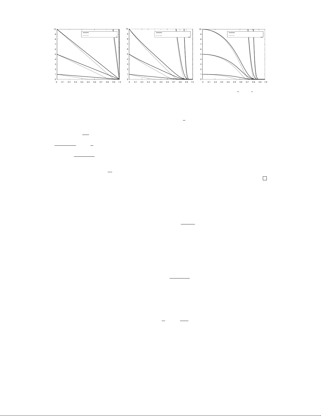
REGULAR P APER Generating new classes of fixed-time stable systems with predefined upp er b ound for the settling time Ro drigo Aldana-L´ op ez a , David G´ omez-Guti ´ errez b,c , Esteban Jim´ enez-Ro dr ´ ıguez d , Juan Diego S´ anchez-T orres e and Michael Defoort f a Departmen t of Computer Science and Systems Engineering, Universit y of Zaragoza, Zaragoza, Spain; b Multi-Agen t Autonomous Systems Lab, Intel Labs, Intel T ecnolog ´ ıa de M ´ exico, Jalisco, Mexico; c T ecnologico de Monterrey , Escuela de Ingenier ´ ıa y Ciencias, Jalisco, Mexico; d Relativit y6 Inc. Computer Science & Artificial In telligence Lab., Jalisco, Mexico; e Researc h Lab oratory on Optimal Design, Devices and Adv anced Materials -OPTIMA-, Departmen t of Mathematics and Ph ysics, ITESO, Jalisco, Mexico; f LAMIH, UMR CNRS 8201, INSA, P olytechnic Universit y of Hauts-de-F rance, V alenciennes, F rance. AR TICLE HISTOR Y Compiled Decem b er 20, 2024 ABSTRA CT This paper aims to pro vide a metho dology for generating autonomous and non- autonomous systems with a fixed-time stable equilibrium p oint where an Upp er Bound of the Settling Time ( UBST ) is set a priori as a parameter of the system. In addition, some conditions for such an upp er bound to b e the least one are pro vided. This construction pro cedure is a relev ant contribution when compared with traditional metho dologies for generating fixed-time algorithms satisfying time constraints since current estimates of an UBST may b e too conserv ativ e. The prop osed methodology is based on time-scale transformations and Lyapuno v analysis. It allows the presentation of a broad class of fixed-time stable systems with predefined UBST , placing them under a common framework with existing metho ds using time-v arying gains. T o illustrate the effectiveness of our approach, w e generate nov el, autonomous and non-autonomous, fixed-time stable algorithms with predefined least UBST . KEYW ORDS Predefined-time systems, fixed-time systems, prescribed-time systems 1. In tro duction In recen t y ears, dynamical systems exhibiting con vergence to their origin in some finite time, indep enden t of the initial condition of the system, ha ve attracted a great deal of atten tion. F or this class of dynamical systems, their origin is said to b e fixed-time stable, which is a stronger notion of finite-time stability (Bhat & Bernstein, 2000; This is the preprint v ersion of the accepted manuscript: Ro drigo Aldana-L´ opez, David G´ omez-Guti ´ errez, Esteban Jim´ enez-Rodr ´ ıguez, Juan Diego S´ anchez-T orres and Michael Defoort “Generating new classes of fixed-time stable systems with predefined upper b ound for the settling time”. International Journal of Con trol. 2021. DOI: 10.1080/00207179.2021.1936190. Please cite the publisher’s version . F or the publisher’s v ersion and full citation details see: https://doi.org/10.1080/00207179.2021.1936190 . The following links pro vide access, for a limited time, to a free copy of the publisher’s version: Link 1. Link 2. Link 3. Link 4. CONT A CT D. G´ omez-Guti ´ errez. Email: david.gomez.g@ieee.org Moula y & P erruquetti, 2006), b ecause in the latter the settling time is, in general, an un b ounded function of the initial condition of the system. This research effort has deriv ed several con tributions on algorithms with the fixed-time con vergence property , suc h as sync hronization of complex netw orks (Khanzadeh & Pourgholi, 2017; X. Liu & Chen, 2016; X. Liu, Ho, Song, & Xu, 2018; Tian, Lu, Zuo, & Y ang, 2018; Y ang, Lam, Ho, & F eng, 2017), stabilizing controllers (Basin, Sh tessel, & Alduk ali, 2016; G´ omez- Guti ´ errez, 2020; P olyak o v, 2012; P olyak o v, Efimo v, & P erruquetti, 2015; S´ anc hez-T orres, Defo ort, & Mu˜ noz V´ azquez, 2020; Zimenk o, Poly ak ov, Efimo v, & P erruquetti, 2018; Zuo, 2019), distributed resource allo cation (Lin, W ang, Li, & Y u, 2019), optimization (Ning, Han, & Zuo, 2017), multi-agen t coordination (Aldana-L´ op ez, G´ omez-Guti´ errez, Defoort, S´ anchez-T orres, & Mu ˜ noz-V´ azquez, 2019; Defo ort, Demesure, Zuo, Poly ako v, & Djemai, 2016; X. Liu, Cao, & Xie, 2019; Shi, Lu, Liu, Huang, & Alssadi, 2018; W ang, Song, Hill, & Krstic, 2018; Zuo & Tie, 2014), state observers (M ´ enard, Moulay , & P erruquetti, 2017), and online differen tiation algorithms (Angulo, Moreno, & F ridman, 2013; Cruz- Za v ala, Moreno, & F ridman, 2011). The fixed-time stability property is of great interest in the developmen t of algorithms for scenarios where real-time constrain ts need to b e satisfied. In fault detection, isolation, and recov ery schemes (T abatabaeip our & Blank e, 2014), failing to reco ver from the fault on time may lead to an unrecov erable mo de. In hybrid dynamical systems, it is frequen tly required that the observer (resp. controller) stabilizes the observ ation error (resp. trac king error) before the next switc hing o ccurs (Defo ort, Djemai, Flo quet, & P erruquetti, 2011; G´ omez-Guti ´ errez, ˇ Celik ovsk´ y, Ram ´ ırez-T revi ˜ no, & Castillo-T oledo, 2015). In the frequency control of an in terconnected p o wer net work, not only is the frequency deviation of interest but also how long the frequency sta ys out of the b ounds (Mishra, Patel, Y u, & Jalili, 2018). A Ly apunov differen tial inequality for an autonomous system to exhibit fixed-time stabilit y w as presented in (Poly ak ov, 2012; Zuo & Tie, 2016), together with an Upp er Bound of the Settling Time ( UBST ) of the system tra jectory . How ev er, suc h an upp er estimate is to o conserv ativ e (Aldana-L´ op ez, G´ omez-Guti´ errez, Jim ´ enez-Ro dr ´ ıguez, S´ anchez-T orres, & Defo ort, 2019). Only recently , non-conserv ativ e UBST has b een deriv ed (Aldana-L´ op ez, G´ omez-Guti´ errez, Jim ´ enez-Ro dr ´ ıguez, et al., 2019; P arsegov, P olyak o v, & Shc herbako v, 2012) for some scenarios. An alternative c haracterization, based on homogeneit y theory , w as prop osed in (Andrieu, Praly , & Astolfi, 2008; P olyak ov, Efimov, & P erruquetti, 2016; Tian, Lu, Zuo, & W ang, 2018). Although it is a p o werful to ol for the design of high order fixed-time stable algorithms, it p oses a c hallenging design problem for time constrained scenarios, since an UBST is often unkno wn. Thus, the design of fixed-time stable systems where an UBST is set a priori explicitly as a parameter of the system, as well as the reduction/elimination of the conserv ativ eness of an UBST , is of great interest. This problem has b een partially addressed for autonomous systems see, e.g., (Aldana-L´ op ez, G´ omez-Guti´ errez, Defo ort, et al., 2019; Aldana-L´ op ez, G´ omez-Guti´ errez, Jim´ enez-Ro dr ´ ıguez, et al., 2019; S´ anc hez-T orres, G´ omez-Guti´ errez, L´ op ez, & Loukiano v, 2018), mainly fo cusing on the class of systems prop osed in (Jim´ enez-Ro dr ´ ıguez, Mu ˜ noz-V´ azquez, S´ anc hez-T orres, & Loukiano v, 2018; Poly ak ov, 2012; S´ anc hez-T orres et al., 2018); and for non-autonomous systems, mainly fo cusing on time-v arying gains that either b ecome singular (Becerra, V´ azquez, Arecha v aleta, & Delfin, 2018; Kan, Y ucelen, Doucette, & Pasiliao, 2017; Morasso, Sanguineti, & Spada, 1997; Song, W ang, & Krstic, 2018; W ang et al., 2018; Y ucelen, Kan, & P asiliao, 2018) or induce Zeno b eha vior (Y. Liu, Zhao, Ren, & Chen, 2018; Ning & Han, 2018) as the predefined-time is reac hed. Con tributions: W e pro vide a metho dology for generating new classes of autonomous 2 and non-autonomous fixed-time stable systems, where an UBST is set a priori explicitly as a parameter of the system. The main result is a sufficient condition in the form of a Ly apunov differen tial inequality , for a nonlinear system to exhibit this prop ert y . Additionally , w e sho w that for any fixed-time stable system with contin uous settling time function there exists a Lyapuno v function satisfying such differen tial inequalit y . Based on this characterization, w e sho w how a fixed-time stable system with predefined UBST can b e constructed from a nonlinear asymptotically stable one, presenting sufficien t conditions for suc h an upp er b ound to b e the least one. T o illustrate our approach, w e pro vide examples sho wing ho w to deriv e autonomous and non-autonomous fixed-time stable systems, with predefined least UBST . This is a significant con tribution to the design of control systems satisfying time constrain ts since, even in the scalar case, the existing UBST estimates are often to o conserv ativ e (Aldana-L´ op ez, G´ omez-Guti´ errez, Jim ´ enez-Ro dr ´ ıguez, et al., 2019). Notation: R is the set of real num b ers, ¯ R = R ∪ {−∞ , + ∞} , R + = { x ∈ R : x ≥ 0 } and ¯ R + = R + ∪ { + ∞} . The Euclidean norm of x ∈ R n is denoted as || x || . h 0 ( z ) = dh ( z ) dz denotes the first deriv ativ e of the function h : R → R . C k ( I ) is the class of functions f : I → R with k ≥ 0 and I ⊆ R whic h has contin uous k -th deriv ativ e in I . F or z ∈ R + , Γ( z ) = R + ∞ 0 e − ξ ξ z − 1 dξ is the Gamma function; for x, a, b ∈ R + , B ( x ; a, b ) = R x 0 ξ a − 1 (1 − ξ ) b − 1 dξ and B − 1 ( · ; · , · ) are the incomplete Beta function and its in verse, resp ectively; for x ∈ R erf ( x ) = R x 0 2 √ π e − ξ 2 dξ is the Error function. F or x > 0, ci ( x ) = − R + ∞ x cos( ξ ) ξ dξ and si ( x ) = − R + ∞ x sin( ξ ) ξ dξ are the cosine and sine integrals resp ectively . K b a is the class of strictly increasing C 1 ((0 , a )) functions h : [0 , a ) → ¯ R with a, b ∈ ¯ R satisfying h (0) = 0 and lim z → a h ( z ) = b . 2. Preliminaries Consider the system ˙ x = − 1 T c f ( x, t ) , ∀ t ≥ t 0 , f (0 , t ) = 0 , (1) where x ∈ R n is the state of the system, T c > 0 is a parameter, t ∈ [ t 0 , + ∞ ) and f : R n × R + → R n , contin uous on x and contin uous almost everywhere on t . The solutions are understo od in the sense of Caratheo dory (O’Regan, 1997). W e assume that f ( · , · ) is such that the origin of system (1) is asymptotically stable and system (1) has the prop erties of existence and uniqueness of solutions in forward-time on the in terv al [ t 0 , + ∞ ) (Khalil & Grizzle, 2002). The solution of (1) for t ≥ t 0 with initial condition x 0 is denoted b y x ( t ; x 0 , t 0 ), and the initial state is giv en b y x ( t 0 ; x 0 , t 0 ) = x 0 . Remark 1. F or simplicit y , throughout the pap er, we assume that the origin is the unique equilibrium point of the systems under consideration. Thus, without ambiguit y , w e refer to the global stability (in the respective sense) of the origin of the system as the stability of the system. The extension to lo cal stability is straightforw ard. Definition 2.1. (P olyak ov & F ridman, 2014)(Settling-time function) The settling- time function of system (1) is defined as T ( x 0 , t 0 ) = inf { ξ ≥ t 0 : lim t → ξ x ( t ; x 0 , t 0 ) = 0 } − t 0 ∈ ¯ R . F or autonomous systems ( f in (1) do es not dep end on t ), the settling-time function 3 is indep enden t of t 0 . Notice that, if the system is exp onen tially stable, then according to Definition 2.1, ∀ x 0 6 = 0, T ( x 0 , t 0 ) = + ∞ . Definition 2.2. (P olyak ov & F ridman, 2014) (Fixed-time stabilit y) System (1) is said to b e fixe d-time stable if it is asymptotically stable (Khalil & Grizzle, 2002) and the settling-time function T ( x 0 , t 0 ) is b ounded on R n × R + , i.e. there exists T max ∈ R + \ { 0 } suc h that T ( x 0 , t 0 ) ≤ T max if t 0 ∈ R + and x 0 ∈ R n . Thus, T max is an UBST of x ( t ; x 0 , t 0 ). W e are in terested on finding sufficien t conditions on system (1) suc h that an UBST is given b y the parameter T c , i.e. T c = T max . Of particular interest is to find suffic ien t conditions such that T c is the least UBST . 2.1. Time-sc ale tr ansformations As in (Pic´ o, Pic´ o-Marco, Vignoni, & De Battista, 2013), the tra jectories corresponding to the system solutions are in terpreted, in the sense of differential geometry (K ¨ uhnel, 2015), as regular parametrized curves. Since w e apply regular parameter transformations o ver the time v ariable, then without am biguit y , this reparametrization is sometimes referred to as time-scaling. Definition 2.3. (K ¨ uhnel, 2015, Definition 2.1) A regular parametrized curve, with parameter t , is a C 1 ( I ) immersion c : I → R , defined on a real in terv al I ⊆ R . This means that dc dt 6 = 0 holds everywhere. Definition 2.4. (K ¨ uhnel, 2015, Pg. 8) (Regular parameter transformation) A regular curv e is an equiv alence class of regular parametrized curves, where the equiv alence relation is giv en by regular (orien tation preserving) parameter transformations ϕ , where ϕ : I → I 0 is C 1 ( I ), bijective and dϕ dt > 0. Therefore, if c : I → R is a regular parametrized curve and ϕ : I → I 0 is a regular parameter transformation, then c and c ◦ ϕ : I 0 → R are considered to b e equiv alen t. 3. Main Results The metho dology presented in this section to obtain fixed-time stable systems with predefined UBST subsumes some existing results, in b oth, the autonomous and the non-autonomous cases. 3.1. Time-sc aling and settling-time c omputation Assumption 3.1. H : R → R is c ontinuous in R , lo c al ly Lipschitz in R \ { 0 } , and satisfies H (0) = 0 and ∀ z ∈ R \ { 0 } , z H ( z ) > 0 . Mor e over, ˜ x ( τ ; x 0 , 0) is the unique solution of the asymptotic al ly stable system d ˜ x dτ = −H ( ˜ x ) , ˜ x (0; x 0 , 0) = x 0 , ˜ x ∈ R , (2) and T ( x 0 , 0) is its settling time. The follo wing lemma presents the construction of the parameter transformation that 4 will b e used hereinafter. Lemma 3.2. Under Assumption 3.1, supp ose that ψ ( τ ) = T c Z τ 0 1 Υ( ˜ x ( ξ ; x 0 , 0) , ψ ( ξ )) dξ , (3) has a unique solution ψ ( τ ) on I 0 = [0 , T ( x 0 , 0)) , wher e T c > 0 , and Υ : R × R + → R + \ { 0 } is a function such that [Υ( x, ˆ t )] − 1 c ontinuous for al l x ∈ R \ { 0 } and ˆ t ∈ R + . Then, the map ψ : I 0 → J , wher e J is the r esulting r ange of ψ ( τ ) , is c ontinuous and bije ctive. Mor e over, the bije ctive function ϕ : I = [ t 0 + inf J , t 0 + sup J ) → I 0 define d by ϕ − 1 ( τ ) = ψ ( τ ) + t 0 is a p ar ameter tr ansformation. F urthermor e, J = [0 , lim τ →T ( x 0 , 0) ψ ( τ )) . Pr o of. Let ψ ( τ ) b e the solution of (3) in I 0 . Since ˜ x ( τ ; x 0 , 0), τ ∈ I 0 , is contin uous, then [Υ( ˜ x ( τ ; x 0 , 0) , ψ ( τ ))] − 1 is contin uous on τ ∈ I 0 and ψ ( τ ) is C 1 ( I 0 ). Moreov er, for all x ∈ R \ { 0 } and ˆ t ∈ R + , Υ( x, ˆ t ) > 0, then it satisfies dψ dτ > 0, hence ψ is injectiv e (Spiv ak, 1965, Pg. 34). On the other hand, lim τ → inf I 0 ψ ( τ ) = inf J and lim τ → sup I 0 ψ ( τ ) = sup J , hence, b y the contin uit y of ψ , ψ is surjectiv e and J = [0 , lim τ →T ( x 0 , 0) ψ ( τ )). Th us, ψ : I 0 → J is bijective. It follows that ϕ is C 1 ( I ), satisfies dϕ dτ > 0 and is bijective. Th us, ϕ : I → I 0 is a parameter transformation. The following lemma sho ws that if (2) has a known settling time function, then the parameter transformation giv en in Lemma 3.2 induces a nonlinear system with known settling-time function. Lemma 3.3. Under Assumption 3.1, supp ose that ψ ( τ ) is the unique solution of (3) on I 0 = [0 , T ( x 0 , 0)) , and let Ψ( z , ˆ t ) =  Υ( z , ˆ t ) for ˆ t ∈ J = [0 , lim τ →T ( x 0 , 0) ψ ( τ )) 1 otherwise with Υ( z , ˆ t ) and T c as in L emma 3.2. Then, the system ˙ x = − 1 T c Ψ( x, ˆ t ) H ( x ) , x ( t 0 ; x 0 , t 0 ) = x 0 , (4) wher e ˆ t = t − t 0 , x ∈ R , has a unique solution x ( t ; x 0 , t 0 ) =  ˜ x ( ϕ ( t ); x 0 , 0) for t ∈ I 0 elsewher e, (5) wher e I = [ t 0 , t 0 + lim τ →T ( x 0 , 0) ψ ( τ )) and ϕ − 1 ( τ ) = ψ ( τ ) + t 0 . Mor e over, (4) is asymptotic al ly stable and the settling time of x ( t ; x 0 , t 0 ) is given by T ( x 0 , t 0 ) = lim τ →T ( x 0 , 0) ψ ( τ ) . (6) Pr o of. Consider the parameter transformation ϕ : I → I 0 giv en in Lemma 3.2 and let x ( t ; x 0 , t 0 ) = ˜ x ( ϕ ( t ); x 0 , 0). Notice that, ˜ x ( τ ; x 0 , 0), τ ∈ I 0 and x ( t ; x 0 , t 0 ), t ∈ I are equiv alen t (in the sense of regular curv es). Moreov er, ˙ x = d dt ˜ x ( ϕ ( t ); x 0 , 0) = d ˜ x dτ   τ = ϕ ( t ) dϕ dt , where d ˜ x dτ   τ = ϕ ( t ) = −H ( ˜ x ( ϕ ( t ); x 0 , 0)) and dϕ dt = T c − 1 Ψ( x ( t ; x 0 , t 0 ) , ˆ t ). Hence, ˙ x = − T c − 1 H ( x ( t ; x 0 , t 0 ))Ψ( x ( t ; x 0 , t 0 ) , ˆ t ), and therefore x ( t ; x 0 , t 0 ) is s olution of 5 (4) on I . Th us, for the solution ˜ x ( τ ; x 0 , 0), τ ∈ I 0 of (2) , the equiv alent curv e x ( t ; x 0 , t 0 ), t ∈ I , under the parameter transformation ϕ , is solution of (4) on I . Moreo ver, since d ˜ x dτ = d dτ ( x ◦ ϕ − 1 )( τ ; x 0 , 0) = −H ( ˜ x ( τ ; x 0 , 0)), then for any solution of (4) on I , there exists an equiv alent curve on I 0 , under the parameter transformation ϕ − 1 , that is solution of (2) . Thus the uniqueness of the solution of (4) on I follo ws from the uniqueness of solutions of (2) . Finally , since ˜ x ( τ ; x 0 , 0) reac hes the origin at τ = T ( x 0 , 0) then, x ( t ; x 0 , t 0 ) reaches the origin at t = t 0 + lim τ →T ( x 0 , 0) ψ ( τ ). Moreov er, since (4) has an equilibrium p oin t at x = 0, then the solution of (4) remains at the origin for all t ∈ [ t 0 + lim τ →T ( x 0 , 0) ψ ( τ ) , + ∞ ). Hence, w e can conclude that (4) is asymptotically stable, (5) is the unique solution in the in terv al [ t 0 , + ∞ ) and the settling time function is giv en by (6). 3.2. Fixe d-time stability of sc alar systems with pr e define d le ast UBST In the rest of the pap er, we analyze the cases where Ψ( x, ˆ t ) is time inv ariant or a function only of t . W e show that in these cases, (3) has a unique solution. Assumption 3.4. L et Φ : R + → ¯ R + \ { 0 } b e a function satisfying Φ(0) = + ∞ , ∀ z ∈ R + \ { 0 } , Φ( z ) < + ∞ and Z + ∞ 0 Φ( z ) dz = 1 . (7) Lemma 3.5. Under Assumption 3.1, let Υ( z , ˆ t ) = (Φ( | z | ) H ( | z | )) − 1 wher e Φ( · ) satisfies Assumption 3.4, then, (3) has a unique solution on I 0 = [0 , T ( x 0 , 0)) , given by ψ ( τ ) = T c Z τ 0 Φ( | ˜ x ( ξ ; x 0 , 0) | ) H ( | ˜ x ( ξ ; x 0 , 0) | ) dξ . (8) Pr o of. Let Υ( z , ˆ t ) = (Φ( | z | ) H ( | z | )) − 1 and notice that Υ( ˜ x ( τ ; x 0 , 0) , ψ ) − 1 is indep enden t of ψ . Therefore, it follo ws that dψ dτ = T c Υ( ˜ x ( τ ; x 0 , 0) , ψ ) − 1 , ψ (0) = 0 (9) has a unique solution giv en b y ψ ( τ ) = T c R τ 0 Φ( | ˜ x ( ξ ; x 0 , 0) | ) H ( | ˜ x ( ξ ; x 0 , 0) | ) dξ . Moreov er, b y (Agarw al & Lakshmik an tham, 1993, Lemma 1.2.2), a solution of (9) is also a solution of (3) and vice versa. Assumption 3.6. L et Φ : R + → ¯ R + \ { 0 } b e a c ontinuous function on R + \ { 0 } satisfying (7) and ∀ τ ∈ R + \ { 0 } , Φ( τ ) < + ∞ . Mor e over, Φ is either non-incr e asing or lo c al ly Lipschitz on R + \ { 0 } . Lemma 3.7. Under Assumption 3.1, let I 0 = [0 , T ( x 0 , 0)) , and c onsider the first or der or dinary differ ential e quation dψ ( τ ) dτ = T c Φ( τ ) , ψ (0) = 0 , τ ∈ I 0 , (10) 6 wher e Φ( · ) satisfies Assumption 3.6, then (10) has a unique solution ψ : I 0 → J = [0 , lim τ →T ( x 0 , 0) ψ ( τ )) , which is bije ctive and given by ψ ( τ ) = T c Z τ 0 Φ( ξ ) dξ , τ ∈ I 0 . (11) Mor e over, let Ψ( z , ˆ t ) = Φ( ψ − 1 ( ˆ t )) then ψ ( τ ) is also the unique solution of (3) on I 0 . Pr o of. It follows that (10) has a unique solution giv en by ψ ( τ ) = T c R τ 0 Φ( ξ ) dξ . Note that ∀ τ ∈ I 0 \ { 0 } , ψ : I 0 → J is C 1 ( I 0 ) with dψ dτ > 0, and ψ (0) = 0, hence ψ is injective (Spiv ak, 1965, Pg. 34). Note that lim τ → inf I 0 ψ ( τ ) = inf J and lim τ → sup I 0 = sup J and, b y contin uity of ψ , ψ is surjectiv e. Hence, ψ : I 0 → J is bijectiv e. Since Φ( ψ − 1 ( ψ ( τ ))) = Φ( τ ), then ψ ( τ ) is a solution of (3) . Now, on the one hand if Φ is non-increasing, then Φ ◦ ψ − 1 is non-increasing. T o show this let a > b , ψ − 1 ( a ) > ψ − 1 ( b ) and Φ( ψ − 1 ( a )) < Φ( ψ − 1 ( b )). On the other hand, if Φ is Lipsc hitz on [ , + ∞ ) , ∀  > 0, then Φ ◦ ψ − 1 is Lipschitz on J \ [0 ,  ). T o show this, note that there exists a constant M Φ > 0 suc h that | Φ( ψ − 1 ( x 1 )) − Φ( ψ − 1 ( x 2 )) | ≤ M Φ | ψ − 1 ( x 1 ) − ψ − 1 ( x 2 ) | ≤ M | x 1 − x 2 | where M = M Φ max x ∈ J \ [0 , ) ( ψ − 1 ) 0 ( x ). Then, in the former (resp. in the latter) case it follo ws from Peano’s uniqueness Theorem (Agarw al & Lakshmik an tham, 1993, Theorem 1.3.1) (resp. from Lipschitz uniqueness Theorem (Agarwal & Lakshmik antham, 1993, Theorem 1.2.4)) that dz dτ = T c Φ( ψ − 1 ( z )) , z (  ) = T c Z  0 Φ( ξ ) dξ , (12) has a unique solution z = ψ ( τ ), ∀ , τ ∈ I 0 \ { 0 } . Since ψ (0) = 0, then (12) with  = 0 has a unique solution z = ψ ( τ ), τ ∈ I 0 . Moreov er, by (Agarw al & Lakshmik an tham, 1993, Lemma 1.2.2), a solution of (12) is a solution of (3) and vice versa. In Lemma 3.8, we presen t a c haracterization for a map Ψ : R × R + → ¯ R + , in the autonomous case, such that system (4) is fixed-time stable with T c as the least UBST . Lemma 3.8. (Char acterization of Ψ( z , ˆ t ) for fixe d-time stability of autonomous systems with pr e define d le ast UBST) Under Assumption 3.1, with Υ( z , ˆ t ) = (Φ( | z | ) H ( | z | )) − 1 (13) wher e ˆ t = t − t 0 and Φ( · ) satisfies Assumption 3.4, system (4) is fixe d time stable with T c as the pr e define d le ast UBST. Pr o of. By Lemma 3.5, (8) is the solution of (3) . Using the change of v ariables z = | ˜ x ( τ ; x 0 , t 0 ) | , (6) leads to T ( x 0 , t 0 ) = T c R | x 0 | 0 Φ( z ) dz . Since Φ( · ) > 0 then T ( x 0 , t 0 ) is increasing with resp ect to | x 0 | . Moreo ver, since Φ( · ) satisfies (7) , the settling-time function satisfies sup ( x 0 ,t 0 ) ∈ R n × R + T ( x 0 , t 0 ) = lim | x 0 |→ + ∞ T c R | x 0 | 0 Φ( z ) dz = T c . The following result states the construction of fixed-time stable non-autonomous systems with predefined UBST . Lemma 3.9. (Char acterization of Ψ( z , ˆ t ) for fixe d-time stability of non-autonomous systems with pr e define d le ast UBST) Under Assumption 3.1, let ψ ( τ ) , τ ∈ I 0 = 7 [0 , T ( x 0 , 0)) , b e the solution of (10) and ψ − 1 ( ˆ t ) its inverse map. Then, with Υ( z , ˆ t ) = 1 Φ( ψ − 1 ( ˆ t )) (14) wher e ˆ t = t − t 0 and Φ( · ) satisfies Assumption 3.6, system (4) is fixe d-time stable with T c as the pr e define d UBST. F urthermor e, (1) the settling time is exactly T c for al l x 0 6 = 0 if T ( x 0 , 0) = + ∞ , for al l x 0 6 = 0 ; (2) T ( x 0 , t 0 ) < T c if T ( x 0 , 0) < + ∞ , but the le ast UBST is T c if, in addition, T ( x 0 , 0) is r adial ly unb ounde d, i.e. T ( x 0 , 0) → + ∞ as | x 0 | → + ∞ . (3) If (2) is fixe d-time stable, then, ther e exists Ψ max < + ∞ such that for al l x 0 and al l t ∈ [ t 0 , t 0 + T ( x 0 , t 0 )] Ψ( z , ˆ t ) ≤ Ψ max . Pr o of. By Lemma 3.7, the solution of (3) is given by (11) . Then, the settling time function of (4) is giv en b y T ( x 0 , t 0 ) = T c R T ( x 0 , 0) 0 Φ( ξ ) dξ . T o show item (1) note that if T ( x 0 , 0) = + ∞ , then T ( x 0 , t 0 ) = T c R + ∞ 0 Φ( ξ ) dξ = T c , ∀ x 0 ∈ R \ { 0 } . T o sho w item (2) note that, since T ( x 0 , 0) < + ∞ then T ( x 0 , t 0 ) = T c R T ( x 0 , 0) 0 Φ( ξ ) dξ < T c . Ho wev er, if T ( x 0 , 0) is radially unbounded, then sup ( x 0 ,t 0 ) ∈ R n × R + T ( x 0 , t 0 ) = lim | x 0 |→ + ∞ T c R T ( x 0 , 0) 0 Φ( ξ ) dξ = T c . Hence, T c is the least UBST . T o show item (3) notice that, since there exists T max < + ∞ , such that for all x 0 ∈ R , T ( x 0 , 0) ≤ T max then ∃ ˆ T c < T c , such that sup ( x 0 ,t 0 ) ∈ R n × R + T ( x 0 , t 0 ) ≤ lim | x 0 |→ + ∞ T c R T max 0 Φ( ξ ) dξ = ˆ T c . Th us, for all t ∈ [ t 0 , t 0 + ˆ T c ], Ψ( z , ˆ t ) ≤ Ψ( z , ˆ T c ) < + ∞ . Remark 2. Fixed-time stability of non-autonomous systems has b een applied for the design of stabilizing con trollers (Song et al., 2018), observers (Hollo wa y & Krstic, 2019), consensus algorithms (Colunga, V´ azquez, Becerra, & G´ omez-Guti ´ errez, 2018; Ning & Han, 2018; W ang, Song, Hill, & Krstic, 2017; W ang et al., 2018) and rob ot con trol (Delfin, Becerra, & Arecha v aleta, 2016) with predefined settling-time at T c , whic h uses time-v arying gains that are either con tinuous in [ t 0 , T c + t 0 ) (Becerra et al., 2018; Morasso et al., 1997; Song et al., 2018; W ang et al., 2018) or piecewise contin uous requiring Zeno behavior (Y. Liu et al., 2018; Ning & Han, 2018) as t approac hes T c + t 0 . Notice that, in this paper, w e fo cus on the former case. Remark 3. In the autonomous case, T c is the least UBST , whereas, in the non- autonomous case, if item (1) is satisfied, ev ery nonzero tra jectory con verges exactly at T c . This feature has b een referred in the literature as predefined-time (Becerra et al., 2018), app ointed-time (Y. Liu et al., 2018) or prescribed-time (W ang et al., 2018). Ho wev er, note that lim t → t 0 + T − c Ψ( z , ˆ t ) = + ∞ , but if item (2) or (3) in Lemma 3.9 is satisfied, then the origin is reac hed b efore the singularit y in Ψ( z , ˆ t ) o ccurs. 3.3. Lyapunov analysis for fixe d time stability with pr e define d UBST The following theorem pro vides a sufficien t condition for a (general) nonlinear system to b e fixed-time stable with predefined UBST . This result follows from the comparison lemma (Khalil & Grizzle, 2002, Lemma 3.4) and the application of the ab ov e results on the time deriv ative of the Ly apunov candidate function. Theorem 3.10. (Lyapunov char acterization for fixe d-time stability with pr e define d UBST) Under Assumption 3.1, if ther e exists a c ontinuous and differ entiable p ositive 8 definite r adial ly unb ounde d function V : R n → R , such that its time-derivative along the tr aje ctories of (1) satisfies ˙ V ( x ) ≤ − 1 T c Ψ( V ( x ) , ˆ t ) H ( V ( x )) , x ∈ R n \ { 0 } , (15) wher e ˆ t = t − t 0 , and Ψ( z , ˆ t ) is char acterize d by the c onditions of L emma 3.8 or L emma 3.9, then, system (1) is fixe d-time stable with T c as the pr e define d UBST. If the e quality in (15) holds, then T c is the le ast UBST. Pr o of. Let w ( t ) b e a function satisfying w ( t ) ≥ 0 and ˙ w = − 1 T c Ψ( w , ˆ t ) H ( w ), and let V ( x 0 ) ≤ w (0). Then, T c is the least UBST of w ( t ). Moreo ver, b y the comparison lemma (Khalil & Grizzle, 2002, Lemma 3.4), it follows that V ( x ( t ; x 0 , t 0 )) ≤ w ( t ). Consequen tly , V ( x ( t ; x 0 , t 0 )) will con v erge to the origin before T c . If (15) is an equalit y and V ( x 0 ) = w (0), then, V ( x ( t ; x 0 , t 0 )) = w ( t ) and T c is the least UBST . Theorem 3.11. If system (1) is autonomous, fixe d-time stable and has a c ontinuous settling time function, then ther e exists a c ontinuous p ositive definite function V : R n → R , such that its time-derivative along the tr aje ctories of (1) satisfies (15) with Ψ( z , ˆ t ) char acterize d by the c onditions of L emma 3.8. If in addition, lim k x 0 k→ + ∞ T ( x 0 , t 0 ) = T c then V ( x ) is r adial ly unb ounde d. Pr o of. Let G ( z ) = T c R z 0 Φ( ξ ) dξ , with Φ( · ) satisfying Assumption 3.4. Note that G 0 ( z ) > 0 , ∀ z ≥ 0 and hence G : R + → [0 , T c ) is a bijection (Spiv ak, 1965, Pg. 34). Moreov er note that G (0) = 0 and lim z →∞ G ( z ) = T c . Hence, V ( x ) = G − 1 ( T ( x, t 0 )) is a contin uous and p ositiv e definite function satisfying V (0) = 0. F urthermore, consider the tra jectory x ( t ; x 0 , t 0 ), then, as noted in (Bhat & Bernstein, 2000, Prop osition 2.4), T ( x ( t ; x 0 , t 0 ) , t 0 ) = max { T ( x 0 , t 0 ) − t, 0 } . Therefore, ˙ V ( x ) = −  G − 1  0 ( T ( x, t 0 )) = − 1 T c Φ( V ( x )) − 1 = − 1 T c Ψ( V ( x ) , ˆ t ) H ( V ( x )) , ∀ x ∈ R n \ { 0 } . It follo ws that, if lim k x 0 k→ + ∞ T ( x 0 , t 0 ) = T c then V ( x ) = G − 1 ( T ( x, t 0 )) is radially un b ounded. The following theorem allo ws generating fixed-time stable systems with predefined UBST from an asymptotically stable ones that has a Ly apunov function satisfying (17) . By construction, suc h V ( x ) will also b e a Lyapuno v function for system (18) satisfying (15). Theorem 3.12. (Gener ating fixe d-time stable systems with pr e define d UBST) Under Assumption 3.1, let the system ˙ y = − g ( y ) , (16) b e asymptotic al ly stable, wher e y ∈ R n , g : R n → R n is c ontinuous and lo c al ly Lipschitz everywher e exc ept, p erhaps, at y = 0 with g (0) = 0 . If ther e exists a Lyapunov function V ( y ) for system (16) such that ˙ V ( y ) ≤ −H ( V ( y )) , ∀ y ∈ R n , (17) then, if Ψ( V ( x ) , ˆ t ) g ( x ) is c ontinuous on x ∈ R n , wher e ˆ t = t − t 0 and Ψ( z , ˆ t ) is a 9 function satisfying the c onditions of L emma 3.8 or L emma 3.9, the system ˙ x = − 1 T c Ψ( V ( x ) , ˆ t ) g ( x ) , x ( t 0 ; x 0 , t 0 ) = x 0 (18) has a unique solution in the interval [ t 0 , + ∞ ) and it is fixe d-time stable with T c as the pr e define d UBST. Pr o of. Since the conditions of Lemma 3.8 or Lemma 3.9 are satisfied, then, (3) has a unique solution. Hence, the pro of of the existence of a unique solution for (18) follo ws b y the same arguments as those of the proof of Lemma 3.3. Let V ( y ) b e a Lyapuno v function candidate for (16) suc h that (17) holds. Therefore, ˙ V ( y ) = − ∂ V ∂ y g ( y ) ≤ −H ( V ( y )), ∀ y ∈ R n . Hence, the evolution of V ( x ) is given b y ˙ V ( x ) = − 1 T c ∂ V ∂ x Ψ( V ( x ) , ˆ t ) g ( x ) ≤ − 1 T c Ψ( V ( x ) , ˆ t ) H ( V ( x )), ∀ x ∈ R n . Hence, by Theorem 3.10, V ( x ( t ; x 0 , t 0 )) conv erges to the origin in fixed-time with T c as the predefined UBST . Notice that, the term Ψ( x, ˆ t ) H ( x ) in (4) is con tinuous at x = 0 with an y choice of Ψ( x, ˆ t ) from either Lemma 3.8 or Lemma 3.9, since H (0) = 0 and [Φ(0)] − 1 = 0. Ho wev er, an arbitrary selection of V ( y ) and Ψ( z , ˆ t ) may lead to a right-hand side of (18) discon tinuous at the origin. A construction from a linear system, guaranteeing con tinuit y of the right-hand side of (18) is provided in the following proposition. Corollary 3.13. L et Ψ( z , t ) define d as in (13) with Φ( z ) satisfying Assumption 3.4 and H ( z ) = (2 λ max ( P )) − 1 z , P ∈ R n × n is the solution of A T P + P A = I with − A ∈ R n × n Hurwitz and λ max ( P ) is the lar gest eigenvalue of P . Then, Ψ( V ( x ) , ˆ t ) Ax , wher e V ( x ) = √ x T P x , is c ontinuous, and the system ˙ x = − 1 T c Ψ( V ( x ) , ˆ t ) Ax (19) wher e ˆ t = t − t 0 , is fixe d-time stable with T c as the pr e define d UBST. Mor e over, if A = αI + S with α a p ositive c onstant and S a skew-symmetric matrix then T c is the le ast UBST. Pr o of. Consider system (16) with g ( y ) = Ay whic h has a Lyapuno v function V ( y ) = p y T P y satisfying ˙ V ≤ − (2 λ max ( P )) − 1 V ( y ) = −H ( V ( y )). Note that, V ( · ) is contin uous and Ψ( · , ˆ t ) is contin uous except at the origin. Therefore, since Ψ(0 , ˆ t ) A (0) = 0, to c heck con tinuit y , it only suffices to sho w that lim k x k→ 0 + k Ψ( V ( x ) , ˆ t ) Ax k = 0 which follo ws from lim k x k→ 0 + k Ψ( V ( x ) , ˆ t ) Ax k 2 = 4 λ max ( P ) 2 lim k x k→ 0 + ( x T A T Ax )( x T P x ) − 1 Φ( V ( x )) − 2 ≤ 4 λ max ( P ) 2 λ max ( A T A ) λ min ( P ) lim k x k→ 0 + Φ( V ( x )) − 2 = 0. Hence, Ψ( V ( x ) , ˆ t ) Ax is contin uous ev erywhere. It follows from Theorem 3.12 that (19) is fixed-time stable with T c as the predefined UBST . Note that, if A = αI + S and P = 1 2 α I , then ˙ V ( y ) = −H ( V ( y )) = − αV ( y ) and ˙ V ( x ) = − 1 T c Ψ( V ( x ) , ˆ t ) H ( V ( x )). Hence, b y Theorem 3.10, (19) is fixed-time stable with T c as the least UBST . Remark 4. Notice that Theorem 3.10 can b e used for the design of first and second order con trollers as in (Aldana-L´ op ez, G´ omez-Guti´ errez, Jim´ enez-Ro dr ´ ıguez, et al., 2019). The design of arbitrary order controllers as in (Mishra et al., 2018). The 10 design of consensus protocols, as in (Aldana-L´ op ez, G´ omez-Guti´ errez, Defo ort, et al., 2019; Ning, Jin, & Zheng, 2017); the design of non-autonomous arbitrary order con trollers as in (G´ omez-Guti´ errez, 2020; Pal, Kamal, Nagar, Bandyopadh y ay , & F ridman, 2020) or the design of non-autonomous state observ ers and online differen tion algorithms (Aldana-L´ op ez, G´ omez-Guti´ errez, Angulo, & Defoort, 2020). 4. Examples of fixed-time stable systems with predefined least UBST 4.1. Examples of autonomous fixe d-time stable systems with pr e define d le ast UBST In this subsection, we present the construction of some examples of Φ( · ) satisfying Assumption 3.4 for generating autonomous fixed time stable systems with predefined least UBST . The result is mainly obtained by applying Corollary 3.13. F or simplicity , w e take A = 1 2 I ∈ R n × n . Prop osition 4.1. L et h ( z ) b e K + ∞ + ∞ . Then, functions Φ( z ) given in T able 1, satisfy Assumption 3.4. Mor e over, the system ˙ x = − 1 T c (Φ( k x k ) k x k ) − 1 x , wher e x ∈ R n and − 1 T c (Φ( k x k ) k x k ) − 1 x shown in T able 1 is fixe d-time stable with T c as the le ast UBST. Pr o of. Note that 1 γ R + ∞ 0 ( αz p + β z q ) − k dz = 1 γ Γ  1 − kp q − p  Γ  kq − 1 q − p  α β  1 − kp q − p α k Γ( k )( q − p ) ! = 1 (Aldana-L´ op ez, G´ omez-Guti ´ errez, Jim ´ enez-Ro dr ´ ıguez, et al., 2019), therefore, b y Prop osition B.1 then Φ( z ) giv en in T able 1- (i) satisfies (7) . Moreo ver, since Φ(0) = + ∞ , then Φ( z ) satisfies Assumption 3.4. In a similar w a y , Φ( z ) giv en in T able 1- (ii) satisfies Assumption 3.4. The pro of that T able 1- (iii) and T able 1- (iv) satisfy (7) follo ws by applying Proposition B.1 to the functions F ( z ) = exp ( − z ), and F ( z ) = 1 ρ ( sin ( z ) + 1)(1 + z ) − 2 (whic h satisfy R + ∞ 0 F ( z ) dz according to Prop osition A.1), resp ectiv ely . The pro of that the system ˙ x = − 1 T c (Φ( k x k ) k x k ) − 1 x with − 1 T c (Φ( k x k ) k x k ) − 1 x sho wn in T able 1 is fixed-time stable with T c as the least UBST follo ws b y applying Corollary 3.13 with g ( x ) = 1 2 x , V ( x ) = k x k , H ( V ( x )) = 1 2 k x k and Φ( z ) giv en in T able 1. Remark 5. The system in T able 1-(i) with h ( z ) = z reduces to the system analyzed in (Lop ez-Ramirez, Efimov, P olyak o v, & Perruquetti, 2019; P olyak o v, 2012). How ev er, here T c is giv en as the predefined least UBST . This feature is a significan t adv an tage with resp ect to (Lop ez-Ramirez et al., 2019; Poly ak ov, 2012), because, as illustrated in (Aldana-L´ op ez, G´ omez-Guti´ errez, Jim ´ enez-Ro dr ´ ıguez, et al., 2019), an UBST pro vided in (P olyak ov, 2012) is to o conserv ativ e. Notice that, the fixed-time stable system with predefined UBST , analyzed in (S´ anc hez-T orres et al., 2018), is found from T able 1-(iii) with h ( z ) = z p with 0 < p < 1. Th us, the algorithms in (Poly ak ov, 2012) and (S´ anchez-T orres et al., 2018) are subsumed in our approach. Example 4.2. F rom T able 1 new classes of fixed-time stable systems with predefined UBST , not present in the literature, can b e derived. F or instance, the systems ˙ x = − γ T c (1 + k x k )( α log(1 + k x k ) p + β log (1 + k x k ) q ) k x k x k (20) 11 x 0 = 0 . 1 x 0 = 1 x 0 = 2 x 0 = 10 e 10 x 0 = 0 . 1 x 0 = 1 x 0 = 2 x 0 = 10 e 10 x 0 = 0 . 1 x 0 = 1 x 0 = 2 x 0 = 10 e 10 time ( t ) time ( t ) time ( t ) Figure 1. Examples of autonomous fixed-time systems with t 0 = 0 and T c = 1 with x ∈ R . F rom left to right: System (20) with α = 1 , β = 2 , p = 0 . 5 , q = 2 and k = 1; System (21); System (22) with p = 1 / 2. and ˙ x = − π 2 T c (exp(2 k x k ) − 1) 1 / 2 x k x k (21) are obtained from T able 1- (i) and T able 1- (ii) with h ( z ) = log (1 + z ) and h ( z ) = z resp ectiv ely . Moreov er, the system ˙ x = − γ (sin( k x k p ) + 2) T c p (1 + k x k p ) 2 x k x k p (22) is obtained from T able 1-(iv) with h ( z ) = z p with 0 < p < 1. Simulations are shown in Figure 1. 4.2. Examples of non-autonomous fixe d-time stable systems with pr e define d le ast UBST In this subsection, we fo cus on the construction of functions Φ( ψ − 1 ( ˆ t )) satisfying the conditions of Lemma 3.9. Based on these functions, w e pro vide some examples of non-autonomous systems, with T c as the settling time for every nonzero tra jectory as w ell as non-autonomous systems with T c as the least UBST . Prop osition 4.3. L et ˆ t = t − t 0 , then with Φ( ψ − 1 ( ˆ t )) given in T able 2, Ψ( z , ˆ t ) given in (14) , satisfies the c onditions of L emma 3.9. Mor e over, the system ˙ x = − 1 T c Ψ( k x k , ˆ t ) x , x ∈ R n , is fixe d-time stable with T c as the settling-time for every nonzer o tr aje ctory. Pr o of. T o show that Ψ( z , ˆ t ) given in T able 2- (i) satisfies the condition of Lemma 3.9, c ho ose h ( z ) = 1 α  1 (1 − η ( z )) α − 1  . Note that h ( z ) is K ∞ T c for α ≥ 0. Therefore, Prop osition B.2 can b e used with α ≥ 0. Hence, choosing Φ( z ) as in Prop osition B.2, leads Φ( ψ − 1 ( ˆ t )) − 1 = T c h 0 ( ˆ t ) = T c η 0 ( ˆ t ) (1 − η ( ˆ t )) α +1 . Note that ψ − 1 ( ˆ t ) is C 1 ([0 , T c )) and η ( ˆ t ) is C 2 ([0 , T c )), then Φ( z ) is C 1 ([0 , + ∞ )), therefore satisfies Assumption 3.6. T o sho w that with Φ( ψ − 1 ( ˆ t )) given in T able 2- (ii) –T able 2- (iv) , Ψ( x, ˆ t ) given in (14) , satisfies the conditions of Lemma 3.9, let F ( z ) = 2 π ( z 2 +1) , F ( z ) = 2 √ π exp  − z 2  and F ( z ) = 1 γ ( αz p + β z q ) − k whic h satisfies R + ∞ 0 F ( z ) dz = 1. If h ( z ) is K ∞ ∞ and C 2 ([0 , + ∞ )), by Prop osition B.1, Φ( z ) = 2 h 0 ( z ) π ( h ( z ) 2 +1) and Φ( z ) = 2 h 0 ( z ) √ π exp  − h ( z ) 2  12 g ( x ) = x g ( x ) = x + b x e 1 2 x 0 = 10 e 2 x 0 = 10 e 5 x 0 = 10 e 2 x 0 = 10 e 5 x 0 = 10 e 2 x 0 = 10 e 5 g ( x ) = x g ( x ) = x + b x e 1 2 g ( x ) = x g ( x ) = x + b x e 1 2 time ( t ) time ( t ) time ( t ) Figure 2. Examples of non-autonomous fixed-time stable system (18) with t 0 = 0, T c = 1, b x e 1 2 = | x | 1 2 sign ( x ) and x ∈ R . F rom left to right. Φ( ψ − 1 ( ˆ t )) − 1 in (23) ; Φ( ψ − 1 ( ˆ t )) − 1 in (24) ; and Φ( ψ − 1 ( ˆ t )) − 1 in (25) with p = 0 . 5, q = 2, α = 1 and β = 2. satisfy Assumption 3.6. F urthermore, since Φ( z ) = 1 γ ( αh ( z ) p + β h ( z ) q ) − k h 0 ( z ) is non- increasing, it satisfies Assumption 3.6. Moreov er, by Prop osition B.1, (11) leads to ψ ( τ ) = 2 T c π arctan ( h ( τ )), ψ ( τ ) = T c erf ( h ( τ )) and using Proposition A.1, ψ ( τ ) = T c ( α/β ) m p γ α k ( q − p ) B   α β h ( τ ) p − q + 1  − 1 ; m p , m q  , resp ectiv ely . Hence, with η ( z ) = h − 1 ( z ) and η 0 ( z ) = 1 h 0 ( h − 1 ( z )) , we obtain Φ( ψ − 1 ( ˆ t )) − 1 giv en in T able 2- (ii) –T able 2- (iv) . F rom the construction of Φ( ψ − 1 ( ˆ t )) − 1 it follows that Ψ( z , ˆ t ) satisfies the conditions of Lemma 3.9. The pro of that ˙ x = − 1 T c Ψ( k x k , ˆ t ) x is a fixed-time stable system with T c as the settling- time for every nonzero tra jectory follo ws from Lemma 3.9- (1) . Remark 6. Let ˆ t = t − t 0 , then with α = 0, Ψ( z , ˆ t ) in T able 2- (i) reduces to the class of TBG prop osed in (Morasso et al., 1997). Particular TBGs , which can be derived from T able 2- (i) , were used in (Becerra et al., 2018; Colunga et al., 2018; Hollow a y & Krstic, 2019; Kan et al., 2017; Pal et al., 2020; Song et al., 2018; W ang et al., 2017; W ang et al., 2018; Y ucelen et al., 2018). Notice that, Theorem 1 in(Pal et al., 2020) is a particular case of Theorem 3.12, where Ψ( x, ˆ t ) = 1 1 − ˆ t/T c , H ( z ) = η (1 − e −| x | ) sig n ( x ), and V ( x ) = | x | , with ˆ t = t − t 0 , t 0 = 0, and η ≥ 1. Notice that with suc h H ( z ), system (2) satisfies, T ( x 0 , 0) = + ∞ for all x 0 ∈ R . Example 4.4. Let ˆ t = t − t 0 , then taking η ( z ) = z /T c and α = 0 in T able 2- (i) results in Φ( ψ − 1 ( ˆ t )) − 1 = 1 1 − ˆ t/T c (23) whic h corresp onds to a TBG . Other time-v arying gains, which are not a TBG are obtained from T able 2- (ii) and T able 2- (iv) by taking η ( z ) = z , which yields to Φ( ψ − 1 ( ˆ t )) − 1 = π 2 sec  π ˆ t 2 T c  2 , (24) and Φ( ψ − 1 ( ˆ t )) − 1 = γ ( α P ( ˆ t ) p + β P ( ˆ t ) q ) k , (25) resp ectiv ely . It follo ws from Lemma 3.9, that taking g ( x ) = x leads to system (18) 13 where all non-zero tra jectories has T c as the settling time (Figure 2 solid-line), whereas taking g ( x ) = x + k x k α − 1 x with 0 < α < 1 leads to system (18) ha ving T c as the least UBST (Figure 2 dotted-line). Th us, for finite initial conditions, the origin is reac hed b efore T c . Sim ulations for the system ˙ x = − 1 T c Ψ( | x | , ˆ t ) g ( x ) using (23) , (24) and (25) , x ∈ R are presented in Figure 2. 4.3. Examples of fixe d-time se c ond or der systems with pr e define d UBST Prop osition 4.5. Assume that, under a suitable sele ction of k 1 , k 2 , g 1 ( · ) and g 2 ( · ) , the system ˙ y 1 = − k 1 g 1 ( y 1 ) + y 2 (26) ˙ y 2 = − k 2 g 2 ( y 1 ) − y 2 (27) is finite-time stable and ther e exists a Lyapunov function V ( y ) , satisfying (17) . Then, the system ˙ z 1 = − κ ( ˆ t ) k 1 g 1 ( z 1 ) + z 2 (28) ˙ z 2 = − κ ( ˆ t ) 2 k 2 g 2 ( z 1 ) (29) wher e κ ( ˆ t ) = 1 T c Ψ( x, ˆ t ) with Ψ( x, ˆ t ) given as in (14) with Φ( ψ − 1 ( ˆ t )) − 1 given in (23) and ˆ t = t − t 0 , is fixe d-time stable with T c as the pr e define d UBST. Pr o of. Consider the co ordinate change z 1 = x 1 and z 2 = κ ( ˆ t ) x 2 . Then, in the new co ordinates the dynamic is represented by ˙ x 1 = 1 T c Ψ( x, ˆ t )[ − k 1 g 1 ( x 1 ) + x 2 ] and ˙ x 2 = 1 T c Ψ( x, ˆ t )[ − k 2 g 2 ( x 1 ) − x 2 ]. Hence, the result follo ws from Theorem 3.12 by taking g ( y ) = [ k 1 g 1 ( y 1 ) − y 2 , k 2 g 2 ( y 1 ) + y 2 ] T . Prop osition 4.6. Assume that, under a suitable sele ction of k 1 , k 2 , g 1 ( · ) and g 2 ( · ) , the system ˙ y 1 = y 2 (30) ˙ y 2 = − k 1 g 1 ( y 1 ) − k 2 g 2 ( y 2 ) − y 2 (31) is finite-time stable and ther e exists a Lyapunov function V ( y ) , satisfying (17) . Then, the system ˙ z 1 = z 2 (32) ˙ z 2 = − κ ( ˆ t ) 2 k 1 g 1 ( z 1 ) − k 2 κ ( ˆ t ) 2 g 2 ( κ ( ˆ t ) − 1 z 2 ) (33) wher e κ ( ˆ t ) = 1 T c Ψ( x, ˆ t ) with Ψ( x, ˆ t ) given as in (14) with Φ( ψ − 1 ( ˆ t )) − 1 given in (23) and ˆ t = t − t 0 , is fixe d-time stable with T c as the pr e define d UBST. Pr o of. The proof is similar to the one given for Prop osition 4.5, considering the co ordinate c hange z 1 = x 1 and z 2 = κ ( ˆ t ) x 2 . Remark 7. Notice that the result in Prop osition 4.5 can b e applied straightforw ardly to the design of predefined-time second-order observ ers, whereas the result in 14 Prop osition 4.6 can b e applied straightforw ardly to the design of second-order predefined- time controllers. These results can b e extended to the high order case. Remark 8. An imp ortan t consequence of Lemma 3.9 is that, based on the settling-time function of (28) (resp. (33) ), T c can b e the least UBST . Moreov er, If (26) (resp. (30) ) is fixed-time stable, then κ ( ˆ t ) is b ounded for all t ∈ [ t 0 , t 0 + T ( x 0 , t 0 )] and all x 0 ∈ R 2 . 5. Conclusions and future w ork W e presented a metho dology for generating fixed-time stable algorithms suc h that an UBST is set a priori explicitly as a parameter of the system, pro ving conditions under whic h suc h upp er b ound is the least one. Our analysis is based on time- scaling and Lyapuno v analysis. W e hav e shown that this approac h subsumes some existing metho dologies for generating autonomous and non-autonomous fixed-time stable systems with predefined UBST and allows to generate new systems with nov el v ector fields. Several examples are given sho wing the effectiveness of the prop osed metho d. As future work, w e consider the application/extension of these results to differen tiators, control and consensus algorithms. App endix A. Auxiliary identities Prop osition A.1. The fol lowing identities ar e satisfie d: i ) R + ∞ 0 sin( z )+ a (1+ z ) 2 dz = a − ci (1) cos (1) − si (1) sin (1) ; ii ) R x 0 ( αz p + β z q ) − k dz = ( α/β ) m p α k ( q − p ) B   α β x p − q + 1  − 1 ; m p , m q  , for k p < 1 , k q > 1 , α, β , p, q , k > 0 , m p = 1 − kp q − p , m q = kq − 1 q − p and a > 1 . Pr o of. i) It follo ws from R + ∞ 0 a (1+ z ) 2 dz = a and the change of v ariables u = 1 + z with integration by parts and the definition of ci ( z ) and si ( z ). ii) It follows by the c hange of v ariables u =  α β x p − q + 1  − 1 using the definition of B ( · ; · , · ) similarly as in (Aldana-L´ op ez, G´ omez-Guti ´ errez, Jim´ enez-Ro dr ´ ıguez, et al., 2019). App endix B. Some results on the construction of Φ( z ) Prop osition B.1. L et h ( · ) b e a K + ∞ + ∞ function and let F : R + → ¯ R { 0 } a function satisfying R + ∞ 0 F ( z ) dz = M . Then, Φ( z ) = 1 M F ( h ( z )) h 0 ( z ) satisfies (7) . F urthermor e, with such Φ( z ) , (11) b e c omes ψ ( τ ) = T c R h ( τ ) 0 F ( ξ ) dξ . Mor e over, if F ( z ) < + ∞ , ∀ z ∈ R + and lim z → 0 + h 0 ( z ) = + ∞ , then Φ( · ) satisfies Assumption 3.4. Pr o of. Using ξ = h ( z ), it follows R + ∞ 0 Φ( z ) dz = 1 M R + ∞ 0 F ( h ( z )) h 0 ( z ) dz = 1 M R + ∞ 0 F ( ξ ) dξ = 1. Moreov er, if F ( z ) < + ∞ , ∀ z ∈ R + and lim z → 0 + h 0 ( z ) = + ∞ , then lim z → 0 + Φ( z ) = F (0) lim z → 0 + h 0 ( z ) = + ∞ . Hence, Φ( · ) satisfies Assumption 3.4. The rest of the proof follo ws from (11) and the change of v ariables u = h ( ξ ). Prop osition B.2. L et h ( z ) b e a K ∞ T c function. Then, the function Φ( z ) char acterize d by Φ( h ( z )) = 1 T c  dh ( z ) dz  − 1 satisfies Assumption 3.6. Mor e over, let Υ( z , ˆ t ) = Φ( ψ − 1 ( ˆ t )) 15 then, the solution of (3) is given by ψ ( τ ) = h − 1 ( τ ) and Φ( ψ − 1 ( ˆ t )) = Φ( h ( ˆ t )) . Pr o of. Using the change of v ariables ξ = h ( z ), R + ∞ 0 Φ( ξ ) dξ = R T c 0 Φ( h ( z )) dh dz dz = 1 T c R T c 0 dz = 1. Then, from Lemma 3.7, (11) is the solution of (3) . Moreov er, ψ ( τ ) = T c R h − 1 ( τ ) 0 Φ( h ( z )) dh dz dz = h − 1 ( τ ). Hence, ψ − 1 ( ˆ t ) = h ( ˆ t ) and Φ( ψ − 1 ( ˆ t )) = Φ( h ( ˆ t )). References Agarw al, R. P ., & Lakshmik antham, V. (1993). Uniqueness and nonuniqueness criteria for or dinary differ ential e quations (V ol. 6). W orld Scientific Publishing Compan y. Aldana-L´ op ez, R., G´ omez-Guti ´ errez, D., Angulo, M. T., & Defoort, M. (2020). A metho dology for designing fixed-time stable systems with a predefined upp er-bound in their settling time. arXiv pr eprint arXiv:2001.06707 . Aldana-L´ op ez, R., G´ omez-Guti´ errez, D., Defo ort, M., S´ anchez-T orres, J. D., & Mu ˜ noz-V´ azquez, A. J. (2019). A class of robust consensus algorithms with predefined-time conv ergence under switching top ologies. Int J R obust Nonlin , 29 (17), 6179-6198. doi: Aldana-L´ opez, R., G´ omez-Guti ´ errez, D., Jim´ enez-Ro dr ´ ıguez, E., S´ anc hez-T orres, J. D., & Defo ort, M. (2019). Enhancing the settling time estimation of a class of fixed-time stable systems. Int J R obust Nonlin , 29 (12), 4135-4148. doi: Andrieu, V., Praly , L., & Astolfi, A. (2008). Homogeneous appro ximation, recursiv e observ er design, and output feedback. SIAM J Contr ol Optim , 47 (4), 1814-1850. Angulo, M. T., Moreno, J. A., & F ridman, L. (2013). Robust exact uniformly conv ergen t arbitrary order differen tiator. Automatic a , 49 (8), 2489–2495. Basin, M., Shtessel, Y., & Alduk ali, F. (2016). Con tinuous finite-and fixed-time high-order regulators. Journal of the F r anklin Institute , 353 (18), 5001–5012. Becerra, H. M., V´ azquez, C. R., Arecha v aleta, G., & Delfin, J. (2018). Predefined-time con vergence control for high-order integrator systems using time base generators. IEEE T Contr Syst T , 26 (5), 1866–1873. Bhat, S. P ., & Bernstein, D. S. (2000). Finite-time stability of con tinuous autonomous systems. SIAM J. Contr ol and Optimization , 38 , 751-766. Colunga, J. A., V´ azquez, C. R., Becerra, H. M., & G´ omez-Guti´ errez, D. (2018). Predefined-time consensus of nonlinear first-order systems using a time base generator. Mathematic al Pr oblems in Engine ering , 2018 . Cruz-Za v ala, E., Moreno, J. A., & F ridman, L. M. (2011, No v). Uniform robust exact differen tiator. IEEE T Automat Contr , 56 (11), 2727-2733. doi: Defo ort, M., Demesure, G., Zuo, Z., Poly ak ov, A., & Djemai, M. (2016). Fixed-time stabilisation and consensus of non-holonomic systems. IET Contr ol The ory & Applic ations , 10 (18), 2497–2505. Defo ort, M., Djemai, M., Flo quet, T., & P erruquetti, W. (2011). Robust finite time observer design for m ulticellular con verters. International Journal of Systems Scienc e , 42 (11), 1859–1868. Delfin, J., Becerra, H. M., & Arec hav aleta, G. (2016). Visual servo walking control for h umanoids with finite-time con vergence and smo oth rob ot velocities. International Journal of Contr ol , 89 (7), 1342–1358. G´ omez-Guti ´ errez, D. (2020). On the design of nonautonomous fixed-time controllers with a predefined upp er b ound of the settling time. International Journal of R obust and Nonline ar Contr ol , 30 (10), 3871-3885. G´ omez-Guti´ errez, D., ˇ Celik ovsk´ y, S., Ram ´ ırez-T revi˜ no, A., & Castillo-T oledo, B. (2015). On the observer design problem for con tinuous-time switched linear systems with unkno wn switc hings. Journal of the F r anklin Institute , 352 , 1595–1612. Hollo wa y, J. C., & Krstic, M. (2019). Prescrib ed-time observ ers for linear systems in observ er canonical form. IEEE T Automat Contr , 1-1. doi: 16 Jim ´ enez-Ro dr ´ ıguez, E., Mu ˜ noz-V´ azquez, A. J., S´ anchez-T orres, J. D., & Loukiano v, A. G. (2018). A note on predefined-time stability . In (V ol. 51, pp. 520–525). Elsevier. Kan, Z., Y ucelen, T., Doucette, E., & Pasiliao, E. (2017). A finite-time consensus framework o ver time-v arying graph top ologies with temp oral constrain ts. Journal of Dynamic Systems, Me asur ement, and Contr ol , 139 (7), 071012. Khalil, H. K., & Grizzle, J. (2002). Nonline ar systems (V ol. 3). Prentice hall Upper Saddle Riv er. Khanzadeh, A., & Pourgholi, M. (2017). Fixed-time sliding mo de con troller design for sync hronization of complex dynamical netw orks. Nonline ar Dynamics , 88 (4), 2637– 2649. K ¨ uhnel, W. (2015). Differ ential ge ometry (3rd ed., V ol. 77). American Mathematical So c. Lin, W.-T., W ang, Y.-W., Li, C., & Y u, X. (2019). Predefined-time optimization for distributed resource allo cation. Journal of the F r anklin Institute . Liu, X., Cao, J., & Xie, C. (2019). Finite-time and fixed-time bipartite consensus of multi-agen t systems under a unified discon tinuous control proto col. Journal of the F r anklin Institute , 356 (2), 734–751. Liu, X., & Chen, T. (2016). Finite-time and fixed-time cluster sync hronization with or without pinning control. IEEE tr ansactions on cyb ernetics , 48 (1), 240–252. Liu, X., Ho, D. W., Song, Q., & Xu, W. (2018). Finite/fixed-time pinning synchronization of complex netw orks with stochastic disturbances. IEEE tr ansactions on cyb ernetics , 49 (6), 2398–2403. Liu, Y., Zhao, Y., Ren, W., & Chen, G. (2018). Appointed-time consensus: Accurate and practical designs. Automatic a , 89 , 425 - 429. Lop ez-Ramirez, F., Efimov, D., Poly ako v, A., & Perruquetti, W. (2019). Conditions for fixed-time stability and stabilization of contin uous autonomous systems. Systems & Contr ol L etters , 129 , 26–35. Mishra, J., P atel, R., Y u, X., & Jalili, M. (2018). Recursive surface structure for fixed-time con vergence with applications to p o wer systems. IET Contr ol The ory & Applic ations , 12 (18), 2595–2604. Morasso, P ., Sanguineti, V., & Spada, G. (1997). A computational theory of targeting mo vemen ts based on force fields and top ology represen ting netw orks. Neur o c omputing , 15 (3-4), 411–434. Moula y , E., & Perruquetti, W. (2006). Finite-time stability and stabilization: State of the art. In C. Edwards, E. F ossas Colet, & L. F ridman (Eds.), A dvanc es in variable structur e and sliding mo de c ontr ol (V ol. 334, p. 23-41). Springer Berlin Heidelb erg. M ´ enard, T., Moula y , E., & Perruquetti, W. (2017). Fixed-time observer with simple gains for uncertain systems. Automatic a , 81 , 438 - 446. Retrieved from http:// www.sciencedirect.com/science/article/pii/S0005109817301826 doi: Ning, B., & Han, Q. (2018). Prescrib ed finite-time consensus tracking for m ulti-agent systems with nonholonomic c hained-form dynamics. IEEE T Automat Contr , 1-1. Ning, B., Han, Q.-L., & Zuo, Z. (2017). Distributed optimization for multiagen t systems: An edge-based fixed-time consensus approach. IEEE tr ansactions on cyb ernetics , 49 (1), 122–132. Ning, B., Jin, J., & Zheng, J. (2017). Fixed-time consensus for multi-agen t systems with discon tinuous inherent dynamics ov er switching top ology . International Journal of Systems Scienc e , 48 (10), 2023–2032. O’Regan, D. (1997). Existenc e the ory for nonline ar or dinary differ ential e quations (V ol. 398). Springer Science & Business Media. P al, A. K., Kamal, S., Nagar, S. K., Bandyopadh ya y , B., & F ridman, L. (2020). Design of con trollers with arbitrary con vergence time. Automatic a , 112 , 108710. P arsegov, S., Poly ako v, A., & Shcherbak ov, P . (2012). Nonlinear fixed-time control proto col for uniform allocation of agents on a segmen t. In De cision and c ontr ol (c dc), 2012 ie e e 51st annual c onfer enc e on (pp. 7732–7737). Pic´ o, J., Pic´ o-Marco, E., Vignoni, A., & De Battista, H. (2013). Stability preserving maps 17 for finite-time con vergence: Sup er-t wisting sliding-mode algorithm. Automatic a , 49 (2), 534–539. P olyak ov, A. (2012). Nonlinear feedbac k design for fixed-time stabilization of linear control systems. IEEE T Automat Contr , 57 (8), 2106–2110. P olyak ov, A., Efimo v, D., & Perruquetti, W. (2015). Finite-time and fixed-time stabilization: Implicit Lyapuno v function approach. A utomatic a , 51 , 332–340. P olyak ov, A., Efimov, D., & Perruquetti, W. (2016). Robust stabilization of MIMO systems in finite/fixed time. Int J R obust Nonlin , 26 (1), 69–90. P olyak ov, A., & F ridman, L. (2014). Stability notions and Lyapuno v functions for sliding mo de con trol systems. J F r ankl Inst , 351 (4), 1831 - 1865. S´ anchez-T orres, J. D., Defoort, M., & Mu ˜ noz V´ azquez, A. J. (2020, Nov ember). Predefined- time stabilization of a class of nonholonomic systems. International of Contr ol , 93 (12), 2941-2948. S´ anchez-T orres, J. D., G´ omez-Guti ´ errez, D., L´ op ez, E., & Loukiano v, A. G. (2018, April). A class of predefined-time stable dynamical systems. IMA Journal of Mathematic al Contr ol and Information , 35 (Suppl 1), i1-i29. Shi, X., Lu, J., Liu, Y., Huang, T., & Alssadi, F. E. (2018). A new class of fixed-time bipartite consensus proto cols for m ulti-agent systems with an tagonistic in teractions. Journal of the F r anklin Institute , 355 (12), 5256–5271. Song, Y., W ang, Y., & Krstic, M. (2018). Time-v arying feedback for stabilization in prescribed finite time. Int J R obust Nonlin . Spiv ak, M. (1965). Calculus on manifolds: A mo dern appr o ach to classic al the or ems of advanc e d c alculus . Addison-W esley. T abatabaeip our, S. M., & Blanke, M. (2014). Calculation of critical fault recov ery time for nonlinear systems based on region of attraction analysis. IF AC Pr o c ee dings V olumes , 47 (3), 6741 - 6746. Retriev ed from http://www.sciencedirect.com/science/ article/pii/S1474667016426716 (19th IF AC W orld Congress) doi: Tian, B., Lu, H., Zuo, Z., & W ang, H. (2018). Fixed-time stabilization of high-order integrator systems with mismatc hed disturbances. Nonline ar Dynamics , 94 (4), 2889–2899. Tian, B., Lu, H., Zuo, Z., & Y ang, W. (2018). Fixed-time leader–follow er output feedback consensus for second-order m ultiagent systems. IEEE tr ansactions on cyb ernetics , 49 (4), 1545–1550. W ang, Y., Song, Y., Hill, D. J., & Krstic, M. (2017, Dec). Prescrib ed finite time consensus of net work ed m ulti-agen t systems. In Ie e e c onfer enc e on de cision and c ontr ol (p. 4088-4093). W ang, Y., Song, Y., Hill, D. J., & Krstic, M. (2018). Prescribed-time consensus and containmen t con trol of netw orked multiagen t systems. IEEE T r ansactions on Cyb ernetics . Y ang, X., Lam, J., Ho, D. W., & F eng, Z. (2017). Fixed-time sync hronization of complex net works with impulsiv e effects via nonc hattering con trol. IEEE T r ansactions on Au tomatic Contr ol , 62 (11), 5511–5521. Y ucelen, T., Kan, Z., & P asiliao, E. L. (2018). Finite-time coop erative engagement. IEEE T Au tomat Contr , 1-1. doi: Zimenk o, K., Poly ako v, A., Efimov, D., & Perruquetti, W. (2018). On simple scheme of finite/fixed-time control design. International Journal of Contr ol , 1–9. Zuo, Z. (2019). Fixed-time stabilization of general linear systems with input dela y . Journal of the F r anklin Institute , 356 (8), 4467–4477. Zuo, Z., & Tie, L. (2014). A new class of finite-time nonlinear consensus proto cols for m ulti-agen t systems. International Journal of Contr ol , 87 (2), 363-370. Zuo, Z., & Tie, L. (2016). Distributed robust finite-time nonlinear consensus proto cols for m ulti-agent systems. International Journal of Systems Scienc e , 47 (6), 1366–1375. 18 Φ( z ) ˙ x = − 1 T c (Φ( k x k ) k x k ) − 1 x Conditions (i) 1 γ ( αh ( z ) p + β h ( z ) q ) − k h 0 ( z ) ˙ x = − γ T c h 0 ( k x k ) ( αh ( k x k ) p + β h ( k x k ) q ) k x k x k γ = Γ  1 − kp q − p  Γ  kq − 1 q − p  α β  1 − kp q − p α k Γ( k )( q − p ) , kp < 1, k q > 1, α, β , p, q , k > 0 (ii) 2 π (exp (2 h ( z )) − 1) − 1 / 2 h 0 ( z ) ˙ x = − π 2 T c h 0 ( k x k ) (exp(2 h ( k x k )) − 1) 1 / 2 x k x k lim z → 0 + h 0 ( z ) = + ∞ (iii) exp ( − h ( z )) h 0 ( z ) ˙ x = − 1 T c h 0 ( k x k ) exp( h ( k x k )) x k x k lim z → 0 + h 0 ( z ) = + ∞ (iv) 1 ρ (sin( h ( z ) + α )(1 + h ( z )) − 2 h 0 ( z ) ˙ x = − ρ (1 + h ( k x k )) 2 T c h 0 ( k x k )(sin( h ( k x k ) + α ) k x k x ρ = α − ci (1) cos (1) − si (1) sin (1), α > 1 and lim z → 0 + h 0 ( z ) = + ∞ T able 1. Examples of Φ( z ) satisfying Assumption 3.4, and fixed-time stable systems with predefined least UBST deriv ed from them. Φ( ψ − 1 ( ˆ t )) − 1 Conditions (i) T c η 0 ( ˆ t )   1 − η ( ˆ t )   − ( α +1) α ≥ 0 and η ( z ) is K 1 T c and C 2 ([0 , T c )) (ii) π 2 sec  π ˆ t 2 T c  2 η 0  tan  π ˆ t 2 T c  η ( z ) is K + ∞ + ∞ and C 2 ([0 , + ∞ )) (iii) √ π 2 η 0  erf − 1  ˆ t T c  exp  erf − 1  ˆ t T c  2  η ( z ) is K + ∞ + ∞ and C 2 ([0 , + ∞ )) (iv) γ ( αP ( ˆ t ) p + β P ( ˆ t ) q ) k η 0 ( P ( ˆ t )) γ = Γ ( m p ) Γ ( m q )  α β  m p α k Γ( k )( q − p ) , kp < 1, kq > 1, α, β , p, q , k > 0, m p = 1 − kp q − p , m q = kq − 1 q − p , η ( z ) is K + ∞ + ∞ , P ( z ) p − q = β α B − 1  Γ( m p )Γ( m q ) z Γ( k ) T c ; m p , m q  − 1 − β α T able 2. Examples of Φ( ψ − 1 ( ˆ t )), ˆ t = t − t 0 satisfying conditions of Lemma 3.9, from which non-autonomous fixed-time stable systems with predefined settling time can b e constructed. Notice that, in each case, lim t → T − c Φ( ψ − 1 ( ˆ t )) − 1 = + ∞ . 19