Modeling and Quantifying the Impact of Wind Power Penetration on Power System Coherency

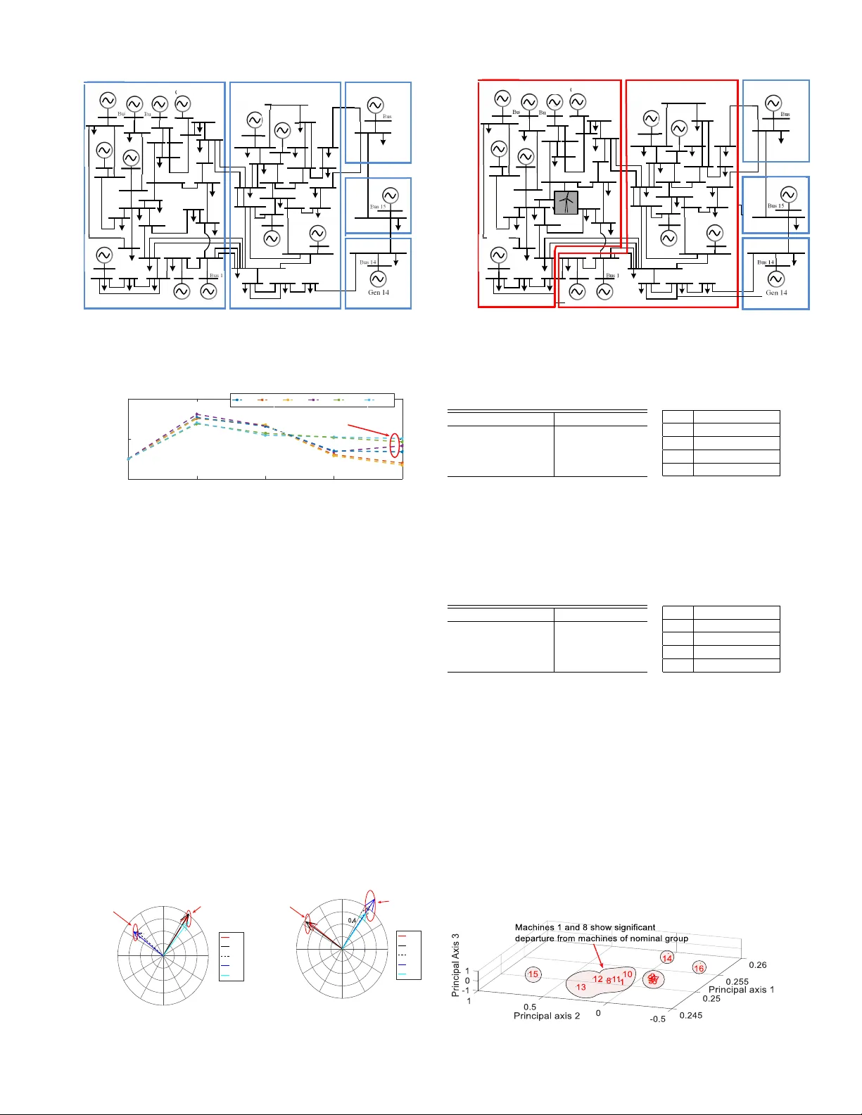
1 Modeling and Quantifying the Impact of W ind Po wer Penetration on Po wer System Coherenc y Sayak Mukherjee 1 , Student Member , IEEE, Aranya Chakrabortty 1 , Senior Member , IEEE, and Saman Babaei 2 , Member , IEEE Abstract —This paper presents a mathematical analysis of how wind generation impacts the coherency property of power systems. Coherency arises from time-scale separation in the dynamics of synchronous generators, where generator states inside a coherent ar ea synchronize o ver a fast time-scale due to str onger coupling, while the areas themselves synchronize over a slower time-scale due to weaker coupling. This time-scale separation is reflected in the form of a spectral separation in the weighted Laplacian matrix describing the swing dynamics of the generators. However , when wind farms with doubly-fed induction generators (DFIG) are integrated in the system then this Laplacian matrix changes based on both the level of wind penetration and the location of the wind farms. The modified Laplacian changes the effective slow eigenspace of the generators. Depending on penetration level, this change may result in changing the identities of the coherent areas. W e dev elop a theoretical framework to quantify this modification, and validate our results with numerical simulations of the IEEE 68 -bus system with one and multiple wind farms. W e compar e our model- based results on clustering with results using measurement-based principal component analysis to substantiate our derivations. Index T erms —Wind power system, coherency , singular pertur- bation, eigen vectors, doubly-fed induction generators. I . I N T RO D U C T I O N O VER the past two decades, significant amount of re- search has been done in studying various impacts of wind po wer penetration on power system dynamics, stability , and control. Results reported in [1]–[3], for example, demon- strate the impact of wind integration on transient stability and small-signal stability . Results in [4] show the low-inertial ef- fects of wind integration resulting in degradation of frequency control. Results in [5] overvie w the effects of penetration lev el of wind farms on the damping characteristics of inter- area oscillations. Multiple studies hav e also been done on dev eloping new control schemes for improving the steady- state and dynamic operation [6], and damping of inter-area oscillations in wind-integrated power systems [7]–[9]. In [10], an analytical framework has been developed to e valuate the effect of wind penetration on time-scale separation properties of power systems that lead to inter-area oscillations. The majority of these w orks describe how wind po wer impacts the eigen values of the small-signal model of a po wer system. Howe ver , in order to understand its holistic ef fect, it is equally 1 S. Mukherjee and A. Chakrabortty are with the Electrical and Computer Engineering Department, North Carolina State Uni versity , Raleigh NC, USA. Emails: { smukher8, achakra2 } @ncsu.edu. 2 S. Babaei is currently with Arriv o Inc., CA, USA. During this research he was with the New Y ork Po wer Authority , White Plains, NY . Email: sbabaei@ncsu.edu. important to ev aluate how the eigen vectors of these models change as more DFIGs penetrate the grid. In this paper we address this problem by studying the impact of wind penetration on a specific eigen-property of power systems that requires the use of eigen vectors - namely , coherency [11], [12]. Coherency is a fundamental property of power systems that arise from the separation of time-scales in the dynamics of synchronous machines. Machines that are strongly coupled tend to swing together, and synchronize ov er a f ast time-scale, thereby forming coherent groups or clusters, while the groups themselves swing against each other and synchronize over a slow time-scale due to their weaker coupling. A large literature e xists on coherency theory , for example see [13]–[16], which to date is still highly useful for transmission planning and operations including dynamic equiv alencing [17], controlled islanding [18], and oscillation damping control [19]. Recent papers such as [20], [21] hav e used data-dri ven techniques to ev aluate how the traditional notions of coherency are affected by non-synchronous power generation from wind, but no theoretical reasonings have been presented. The results deri ved in this paper compensate for this gap by inferring that the intrusion of DFIGs can be vie wed as an addition of heterogeneity to the homogeneous dynamics of synchronous machines. This heterogeneity changes the ef- fective dynamic coupling between the synchronous machines, and thereby perturbs the eigen values and eigen vectors of the swing dynamics such that the coherent groups change. The change depends on the amount of wind power injected, and the b us locations of the wind farms. The main contributions of the w ork can be summarized as follows. W e compare electro-mechanical models of multi- machine power systems both with and without wind injection, and quantify the perturbation caused by this injection in the weighted Laplacian matrix associated with the swing dynamics of the synchronous generators. The quantification is done in terms of both penetration level and location of wind plants. Using singular perturbation theory , an equivalent Laplacian matrix is deriv ed to capture the modified interaction between the synchronous generators in presence of wind. Thereafter , a coherency grouping algorithm is stated in terms of the eigen vectors of this modified Laplacian matrix. A motiv ational example for the study is drawn from the model of the New Y ork state power grid with large-scale wind penetration. The theoretical analyses and algorithms are all verified using simulations of the IEEE benchmark 16-machine, 68-bus power system model with multiple wind plants. 2 I I . R E C A P I T U L A T I O N O F C O H E R E N C Y W e first recall the fundamental theory of coherency in synchronous machines, as detailed in [11]. Consider a power system with m buses and n synchronous generators. Con- sidering classical model of synchronous generators [22], the dynamics of the i th generator can be written as, ˙ δ i = ω i , M i ˙ ω i = P mi − E i x 0 di ( V i Re sin δ i − V i I m cos δ i ) , (1) where δ i , ω i , M i , x 0 di , E i , P mi are respecti vely the phase angle, machine speed deviation from nominal speed ( 120 π rad/s), inertia, direct-axis transient reactance, internal machine voltage, and the mechanical power input to generator i ( i = 1 , . . . , n ) . V i Re and V i I m are the real and imaginary parts of the bus voltage phasor . The acti ve and reactiv e power outputs of the i th generator can be written as, P si = E i x 0 di ( V i Re sin δ i − V i I m cos δ i ) , (2a) Q si = E 2 i x 0 di − E i x 0 di ( V i Re cos δ i − V i I m sin δ i ) . (2b) The acti ve and reacti ve power flow balance at an y bus j , j = 1 , . . . , m can be written as, 0 = P ej − Re    N X k =1 ,k 6 = j V j ( V j k B j k ) ∗    − V 2 j G j , (3a) 0 = Q ej − Im    N X k =1 ,k 6 = j V j ( V j k B j k ) ∗    − V 2 j B j , (3b) where G j and B j are the conductance and the susceptance of the shunt load at bus j with line charging. Assuming the transmission lines to be lossless, B j k denotes the susceptance of the tie-line connecting bus j and bus k . Linearizing (1) and (2) about a stable operating point p 0 = { δ 0 , 0 , V Re 0 , V I m 0 } gov erned by the po wer flow solution we get, ∆ ˙ δ = I ∆ ω , M ∆ ˙ ω = K 11 ∆ δ + K 12 ∆ V + ∆ P m , (4a) ∆ P s = − K 11 ∆ δ − K 12 ∆ V , ∆ Q s = − K 21 ∆ δ − K 22 ∆ V . (4b) Here, M is the diagonal matrix of the machine iner- tias, K ij , i, j = { 1 , 2 } are the Jacobian matrices of appropriate dimensions follo wing from (1)-(3), and I is the identity matrix. ∆ δ, ∆ ω , ∆ P m , ∆ P s , ∆ Q s and ∆ V are the v ectors constructed by stacking the state, the input and the algebraic variables. Specifically , ∆ V = [∆ V 1 Re . . . ∆ V m Re ∆ V 1 I m . . . ∆ V m I m ] T . Following Kron- reduction, and the unforced small-signal model (4) can be written as ∆ ¨ δ = M − 1 ( K 11 − K 12 A − 1 3 A 1 ) | {z } L 0 ∆ δ, (5) A 3 = h ( − K 1 − K 12 ) T K 0 T 1 ( − K 2 − K 22 ) T K 0 T 2 i T A 1 = h − K T 11 0 − K T 21 0 i T . The Jacobian matrices K 1 , K 2 follow from the linearization of (3) for the generator buses, while K 0 1 , K 0 2 are those for non-generator b uses. W e impose a two-time scale behavior on (5) by assuming the network to be di vided into r distinct and non-overlapping coherent areas [11]. The two time-scale model can be deri ved as follows. Let there be n α generators in area α, α = 1 , . . . , r . Let ∆ δ α i and M α i be the small-signal phase angle and inertia of the i th machine in area α . Define two variables q α s ∈ R , q α f = col ( q α f j ) ∈ R n α − 1 for α = 1 , . . . , r, j = 2 , . . . , n α as, q α s = P n α i =1 M α i ∆ δ α i M α , q α f j = ∆ δ α j − ∆ δ α 1 , (6) where M α = P n α i =1 M α i . Stacking q α s and q α f into vectors for α = 1 , . . . , r , one can write,  q s q f  =  ˆ M − 1 U T M G  ∆ δ :=  C G  ∆ δ, (7) where, ˆ M = diag ( M 1 , M 2 , .., M r ) , U = block diag ( U 1 , U 2 , .., U r ) with U α ∈ R n α being the vector of all ones, G = block diag ( G 1 , G 2 , .., G r ) where definition of G α can be found in [11]. The transformation (7) is in vertible with the in verse giv en by [ U G T ( GG T ) − 1 ] . Using (7), one can re write (5) in the time-scale separated form,  ¨ q s ¨ q f  =  T 11 T 12 T 21 T 22   q s q f  := T  q s q f  , (8) T 11 = C M − 1 L E 0 U, T 12 = C M − 1 L E 0 G † , T 21 = GM − 1 L E 0 U, (9) T 22 = GM − 1 ( L I 0 ) G † + GM − 1 L E 0 G † , (10) where G † = G T ( GG T ) − 1 , the matrices L I 0 , L E 0 follow from partitioning L 0 as L 0 = L I 0 +  L E 0 , (11) and 0 <   1 is a singular perturbation parameter arising from the worst-case ratio of the tie-line reactances internal and external to the coherent areas. For precise definition of  , please see [11]. The model (8) is in the singularly perturbed form where q s , q f are the slow and fast variables. For small values of  , (5) will e xhibit a two time-scale behavior , reflected through one DC mode, n − r fast oscillation modes, and r − 1 slo w oscillation modes. The r coherent groups can be identified from the eigen-analysis of M − 1 L 0 . Algorithm 1 as in [11] recalls the steps for this identification. Algorithm 1 Coherency Identification 1. Assuming M and L 0 to be known, compute ( r − 1) smallest eigenv alues (in magnitude) of M − 1 L 0 . Construct V , a matrix whose columns are the eigen vectors of the zero eigen value and these eigen values of M − 1 L 0 . 2. Apply Gaussian elimination with full pivoting to V . From the pivots obtain identity of the reference generators. 3. Permute the rows of V to form V r =  V r 1 V r 2  , where V r 1 are the rows of V corresponding to the reference machines in order , and V r 2 are the remaining rows of V in order . 4. Construct L := V r 2 × V − 1 r 1 . The rows and columns of L correspond to the indices of generators and areas respectively . Let i ∗ = argmax i | L ( i, j ) | for a particular j . Then the generator corresponding to the i ∗ th row of L belongs to coherent area j . I I I . M OT I V AT I N G E X A M P L E W e next provide a motiv ating example from the Ne w Y ork State (NYS) power grid to show how wind penetration can change coherency . The utility-scale model of the NYS grid is simulated using the PSS/E. The model consists of ov er 3 70,000 b uses, and thousands of dynamic elements. The grid is divided into ele ven zones following the NYISO zonal separation based on the similarity of frequency responses of generators in any zone follo wing contingencies. In each zone, a representati ve b us is chosen corresponding to the lar gest generating unit. The system is excited with different NYISO- specified contingencies. Time responses of the frequencies at these b uses are recorded in a matrix M ∈ R ρ × s . F or this example ρ = 11 is the number of representativ e buses, and s = 3571 is the number of data samples. The simulations were run for 15 seconds following the contingencies, and a sampling time of 0 . 0042 second was used. Next, Principal Component Analysis (PCA) [23] is applied on M with the objecti ve of expressing this matrix as M = KV T where columns of V are orthonormal basis vectors. T o achiev e this the following steps are applied. Step 1: The singular v alue decomposition of M is computed as M = U Σ V T where U ∈ R ρ × ρ and V ∈ R s × s are respectively the matrices of left and right singular vectors, and Σ ∈ R ρ × s is the diagonal matrix of singular values. Step 2: Since the columns of V are the normalized right eigen vectors of M T M , one can write K = U Σ , V T = V T . Step 3: The columns of K ∈ R ρ × s represent the weighting for each principal component. Since s  ρ , M can be expected to be a lo w rank matrix. The weightings for c dominant principal axes of M (for any chosen c ) can be found by identifying the c columns of K that hav e highest variance. These c columns of K are finally plotted in a c -dimensional plot. For our example we consider two scenarios A and B, where the wind penetration in the NYS model is respectively 10% and 8% of the nameplate wind capacity . Most of the wind generation is located in zone 1 (western NY) and zones 2 - 5 (central-northern NY). PCA results for these scenarios are shown in Figs. 1-2 for the same contingency , considering c = 2 principal axes. From the two figures it can be seen that subsystem 1 in scenario A moves towards the group formed by subsystems 2 through 5 in scenario B. On the other hand, subsystem 10 departs from its own coherent group in scenario A, and forms a separate cluster in the scenario B. Fig. 1: PCA weightings for scenario A Fig. 2: PCA weightings for scenario B This example shows that depending on operating conditions wind penetration can result in changes in coherent clusters. In the next sections we deri ve conditions that quantify this mov ement depending on the amount and the location of wind penetration for the po wer system model (5). I V . Q U A N T I FI C A T I O N O F P E RT U R B A T I O N A. W ind farm (WF) model Consider the m -bus po wer system model introduced in Section II. W ithout loss of generality we assume that a wind farm is connected at the ( n + 1) th bus. Follo wing [10], the farm is assumed to consist of parallel combinations of γ indi vidual wind turbine and DFIG units. The turbine model is considered as J r ˙ ω r ( t ) = B dt N g ω g ( t ) − K dt θ T ( t ) − ( B dt + B r ) ω r ( t ) + T a ( t ) , (12a) J g ˙ ω g ( t ) = B dt N g ω r ( t ) + K dt N g θ T ( t ) −  B dt N 2 g + B g  ω g ( t ) − T g ( t ) , (12b) ˙ θ T ( t ) = ω r ( t ) − 1 N g ω g ( t ) , (12c) where T a ( t ) = ρA s ν 3 ( t ) C p 2 ω r ( t ) is the aerodynamic torque input. The physical meanings of all variables can be found in [10]. The DFIG dynamics can be expressed in a po wer-in variant synchronously rotating d-q reference frame as v ds = R s i ds + d dt ψ ds − ω e ψ q s , v q s = R s i q s + d dt ψ q s + ω e ψ ds , v dr = R r i dr + d dt ψ dr − ( ω e − ω g e ) ψ q r , v q r = R r i q r + d dt ψ q r + ( ω e − ω g e ) ψ dr , (13) where expressions for flux linkages and the generated electri- cal torque are gi ven by ψ q s = L ls i q s + L m ( i q s + i q r ) , ψ ds = L ls i ds + L m ( i ds + i dr ) , ψ q r = L lr i q r + L m ( i q s + i q r ) , ψ dr = L lr i dr + L m ( i ds + i dr ) , T g ( t ) = 3 2 p 2 L m [ i q s ( t ) i dr ( t ) − i ds ( t ) i q r ( t )] . (14) Here, ω g e := p e 2 ω g is the electrical speed of the rotor of the DFIG, p e is the number of electrical poles. L ls , L lr , L m are the stator and rotor leakage inductances and the magnetizing inductance, respectiv ely . Standard meanings of the voltage and flux variables can be found in [10] and are skipped here for brevity . The active and reactiv e power output of the wind farm can be written as P w = γ ( v q s i q s + v ds i ds ) , Q w = γ ( − v ds i q s + v q s i ds ) . (15a) Aligning v q s with the wind bus voltage phasor, we hav e v q s = | V n +1 | and v ds = 0 . The DFIG is equipped with acti ve and reacti ve po wer control loops with PI controllers whose setpoints are computed using Maximum Power Point Tracking (MPPT) and po wer flow calculations, respectively . 4 B. Linearized wind-inte grated model Since the stator of the DFIG is directly connected to the wind bus through a step-up transformer, the swing states of the synchronous generators will now be dynamically coupled with the wind farm states z which are considered to be the average of the indi vidual unit states [10]. Let the operating point of the power system after wind integration be denoted as ˆ p 0 = { ˆ δ 0 , 0 , z 0 , ˆ V Re 0 , ˆ V I m 0 } . Equations (1) and (2) are linearized about ˆ p 0 as ∆ ˙ δ = I ∆ ω , M ∆ ˙ ω = ¯ K 11 ∆ δ + ¯ K 12 ∆ V + ∆ P m , (16a) ∆ P s = − ¯ K 11 ∆ δ − ¯ K 12 ∆ V , ∆ Q s = − ¯ K 21 ∆ δ − ¯ K 22 ∆ V . (16b) The Jacobians ¯ K ij are different than K ij in (4) due to the shift in operating point from the wind injection. The linearized wind farm model from (12)-(14) around ˆ p 0 is written as ∆ ˙ z = A ∆ z + B ∆ V . (17) Expressions for A and B are skipped for bre vity . Note that B is a zero padded matrix where zeros correspond to the non- wind buses. The linearised power output equations are written as  ∆ P w ∆ Q w  =  C 1 ∆ z C 2 ∆ z  +  D 1 ∆ V D 2 ∆ V  , (18) C 1 = ∂ P w ∂ z    ˆ p 0 , C 2 = ∂ Q w ∂ z    ˆ p 0 , D 1 = ∂ P w ∂ V    ˆ p 0 , D 2 = ∂ Q w ∂ V    ˆ p 0 . The zero-padded matrices D 1 and D 2 depend on wind pen- etration level γ and on the location of the wind farm. More detailed structures of D 1 and D 2 will be shown shortly . The nonlinear power flow equations (3) are linearized at ˆ p 0 with Jacobian matrices ¯ K 1 , ¯ K 2 for activ e and reactive power flows for synchronous generator buses, ¯ K 3 , ¯ K 4 for wind generator bus, and ¯ K 5 , ¯ K 6 for the non-generator b uses as 0 = ¯ A 1 ∆ δ + ¯ A 2 ∆ z + ¯ A 3 ∆ V , (19) ¯ A 1 = [ − ¯ K T 11 0 0 − ¯ K T 21 0 0] T , ¯ A 2 = [0 C 1 0 0 C 2 0] T , ¯ A 3 = [  − ¯ K 1 − ¯ K 12  T ( D 1 − ¯ K 3 ) ¯ K T 5  − ¯ K 2 − ¯ K 22  T ( D 2 − ¯ K 4 ) ¯ K T 6 ] T . Using (16a), (17) and (19), considering ∆ P m = 0 we write the final set of state-space equations for the unforced wind- integrated power system model:   ∆ ˙ δ ∆ ˙ ω ∆ ˙ z   =   0 I 0 R 1 0 R 2 R 3 0 R 4     ∆ δ ∆ ω ∆ z   , (20) where, R 1 = M − 1 ( ¯ K 11 − ¯ K 12 ¯ A − 1 3 ¯ A 1 ) , R 2 = M − 1 ( − ¯ K 12 ¯ A − 1 3 ¯ A 2 ) , R 3 = − B ¯ A − 1 3 ¯ A 1 , R 4 = A − B ¯ A − 1 3 ¯ A 2 . W e next quantify the perturbation of the wind-integrated model (20) from the wind-less model (5). Note that R 1 = M − 1 L where L = ( ¯ K 11 − ¯ K 12 ¯ A − 1 3 ¯ A 1 ) mimics the role of L 0 in (5). Howe ver , unlike L 0 , which is a weighted Laplacian matrix (by definition, a symmetric matrix L 0 = L T 0 is Laplacian if the diagonal entry of each row equals to the negati ve sum of the other entries of that row), L is not a Laplacian matrix. T o quantify the dif ference between L 0 and L , we must compare each of their constituent matrices separately . This is shown as follo ws. C. Quantification of perturbation in L • Perturbation in K 11 and K 12 : The nominal Jacobian matrices K 11 , K 12 are perturbed because of the shift in operating point from p 0 to ˆ p 0 . W e write this perturbation as ¯ K 11 = K 11 + ∆ k 11 ( γ ) , ¯ K 12 = K 12 + ∆ k 12 ( γ ) . (21) The unstructured perturbations ∆ k 11 ( γ ) , ∆ k 12 ( γ ) are im- plicit functions of γ and the location of wind farm, and can be determined numerically for a particular wind integration scenario. • Perturbation in A 3 : The matrices K 0 1 and K 0 2 in (5) are rewritten as K 0 1 = [ − K 3 K 5 ] , K 0 2 = [ − K 4 K 6 ] where K 3 , K 4 are the Jacobians after linearizing (3) for the nominal model with respect to the ( n + 1) th bus voltage, and K 5 , K 6 are that with respect to the voltages of non-generator buses. T o compare A 3 and ¯ A 3 we need to consider the structures of D 1 and D 2 . The entries of D 1 , D 2 can be partitioned in terms of synchronous generator , wind farm and non- generator b uses as follo ws: D 1 =       ( n + 1) ↓ ( n + m + 1) ↓ 0 |{z} sync-gens 1 × n ∂ P w ∂ V ( n +1) Re    ˆ p 0 | {z } wind gen (1 × 1) 0 |{z} non-gens 1 × ( m − n − 1) 0 ∂ P w ∂ V ( n +1) I m    ˆ p 0 0       , D 2 =       ( n + 1) ↓ ( n + m + 1) ↓ 0 |{z} sync-gens (1 × n ) ∂ Q w ∂ V ( n +1) Re    ˆ p 0 | {z } wind gen (1 × 1) 0 |{z} non-gens 1 × ( m − n − 1) 0 ∂ Q w ∂ V ( n +1) I m    ˆ p 0 0       . Simple calculations show that the partial deriv ativ es in the above matrices can be written as ∂ P w ∂ V ( n +1) Re    ˆ p 0 := γ ζ 1 , ∂ P w ∂ V ( n +1) I m    ˆ p 0 := γ ζ 2 , ∂ Q w ∂ V ( n +1) Re    ˆ p 0 := γ ζ 3 , ∂ Q w ∂ V ( n +1) I m    ˆ p 0 := γ ζ 4 , where ζ i ’ s are linearization constants depending on the steady-state stator voltage and stator currents of the DFIG. Using the structures of D 1 and D 2 , we can write: ¯ A 3 = A 3 + γ A 0 3 + ∆ A 3 ( γ ) , (22) where the perturbation term A 0 3 has the following sparse structure, A 0 3 =         ( n + 1) ↓ ( n + m + 1) ↓ . . . . . . . . . . . . . . . . . . ( n + 1) → . . . ζ 1 . . . . . . ζ 2 . . . . . . . . . . . . . . . . . . . . . ( n + m + 1) → . . . ζ 3 . . . . . . ζ 4 . . . . . . . . . . . . . . . . . . . . .         , and ∆ A 3 ( γ ) captures the change in the nominal Jacobians K 12 , K 22 and K i , i = 1 , . . . , 6 due to the operating point shift. • Perturbation in A 1 : T o compare A 1 in (5) with ¯ A 1 in (19), we use (21). W e write the perturbation as ¯ A 1 = A 1 + ∆ A 1 ( γ ) , (23) 5 where ∆ A 1 ( γ ) = [∆ T k 11 0 0 ∆ T k 12 0 0] T follows from (21). • Perturbation in L 0 : W e recall from (20) and (5) that L = ¯ K 11 − ¯ K 12 ¯ A − 1 3 ¯ A 1 and L 0 = K 11 − K 12 A − 1 3 A 1 . Using the matrix inv ersion lemma we get, ¯ A − 1 3 = ( A 3 + γ A 0 3 + ∆ A 3 ( γ )) − 1 = A − 1 3 + X, (24) where X = − ( I + A − 1 3 ( γ A 0 3 + ∆ A 3 ( γ ))) − 1 A − 1 3 ( γ A 0 3 + ∆ A 3 ( γ )) A − 1 3 . Using (21)-(23) we get, L = (( K 11 + ∆ k 11 ) − ( K 12 + ∆ k 12 )( A − 1 3 + X )( A 1 + ∆ A 1 )) , = L 0 − K 12 X A 1 + κ L ( γ ) | {z } Perturbation: ∆ L 0 . (25) Here κ L ( γ ) = ∆ k 11 − K 12 ∆ A 1 − ∆ k 12 ( A − 1 3 + X )( A 1 + ∆ A 1 )) , contains all the terms due to change in operating point, while the perturbation term − K 12 X A 1 contains explicit information about penetration level and location of the wind f arm. D. Extension to multiple wind farms Equations (21)-(25) provide the e xpressions for matrix per - turbations when there is only one wind farm in the system at the ( n + 1) th bus. The approach can be easily extended to when the system has p wind farms, say at ( n + 1 , n + 2 , . . . , n + p ) th buses. Let their penetration lev els be γ 1 , γ 2 , . . . , γ p , respec- tiv ely . W e consider the matrix D 1 = [ D Re 1 , D I m 1 ] , where D Re 1 ∈ R p × m is gi ven by D Re 1 =          ( n + 1) ↓ ( n + 2) ↓ ( n + p ) ↓ . . . ∂ P w ∂ V ( n +1) Re . . . . . . . . . . . . . . . . . . ∂ P w ∂ V ( n +2) Re . . . . . . . . . . . . . . . . . . . . . . . . . . . . . . . . . . . . . . . ∂ P w ∂ V ( n + p ) Re . . .          . (26) The definition of D I m 1 is the same as (26) b ut with V i Re replaced by V i I m , i = n + 1 , . . . , n + p . Similarly , D 2 = [ D Re 2 , D I m 2 ] can be defined in the same way by replacing P w by Q w in (26). As before, the partial deri vati ves are written as ∂ P w ∂ V i Re = γ i ζ 1 i , ∂ P w ∂ V i I m = γ i ζ 2 i , ∂ Q w ∂ V i Re = γ i ζ 3 i , ∂ Q w ∂ V i I m = γ i ζ 4 i , i = n + 1 , . . . , n + p . Accordingly , the admittance matrix ¯ A 3 is expressed as ¯ A 3 = A 3 + γ 1 A 1 3 + γ 2 A 2 3 + · · · + γ p A p 3 + ∆ A 3 ( γ ) , (27) where A i 3 has the same structure as A 0 3 in (22) b ut with ζ 1 , ζ 2 , ζ 3 , ζ 4 replaced by ζ 1 i , ζ 2 i , ζ 3 i , ζ 4 i , respectiv ely . The comparison between L and L 0 follows thereafter in the same way as in the foregoing subsection. V . P E RT U R B A T I O N A NA LY S I S F O R T W O T I M E - S C A L E P RO P E RT Y W e recall from (11), that L 0 = L I 0 +  L E 0 . W e next analyze how the perturbation in L 0 as gi ven by (25) extends to its the internal and external connection components L I 0 and L E 0 , respectiv ely . A. P erturbation in L I 0 and L E 0 Due to the existence of r clusters one can separate A 3 into internal and external admittance matrices as, A 3 = A I 3 + A E 3 . Using exponential expansion we can write, A − 1 3 = ( A I 3 + A E 3 ) − 1 = ( A I 3 ) − 1 + X 1  , (28) where X 1  = [( − ( A I 3 ) − 1 ( A E 3 ) +  (( A I 3 ) − 1 ( A E 3 )) 2 − . . . )( A I 3 ) − 1 ] . Considering a single wind farm scenario we recall (25) as L = L I 0 +  L E 0 − K 12 X A 1 + κ L ( γ ) . (29) The matrix X can be written as X = − ( I + A − 1 3 x ) − 1 A − 1 3 xA − 1 3 , (30) where x = ( γ A 0 3 ) + ∆ A 3 . Expanding ( I + A − 1 3 x ) − 1 we get, ( I + A − 1 3 x ) − 1 = P − 1 1 a + X 2  , (31) where P 1 a = I + ( A I 3 ) − 1 x , and X 2  has the same structure as X 1  with A I 3 , A E 3 replaced by P 1 a and X 1  x , respecti vely . In that case, we ha ve X = − ( P − 1 1 a + X 2  )(( A I 3 ) − 1 + X 1  ) x (( A I 3 ) − 1 + X 1  ) , = − ( P a + P b ) . (32) Here, P a = P − 1 1 a ( A I 3 ) − 1 x ( A I 3 ) − 1 and P b = X 2  (( A I 3 ) − 1 + X 1  ) x (( A I 3 ) − 1 + X 1  ) + P − 1 1 a X 1  x (( A I 3 ) − 1 + X 1  ) . Then finally (25) can be rewritten as L = L I 0 +  L E 0 + K 12 P a A 1 + K 12 P b A 1 + κ L ( γ ) , (33) = ( L I 0 + ∆ L I ) +  ( L E 0 + ∆ L E ) , (34) where ∆ L I = K 12 P a A 1 + κ L ( γ ) , ∆ L E = K 12 P b A 1 . These perturbations, which are functions of γ and the wind f arm location, quantify the changes in the internal and external components of L 0 . B. Extraction of the equivalent Laplacian W e next substitute the expression (34) in R 1 = M − 1 L in the wind-integrated model (20). From this model we can write ∆ ¨ δ = M − 1 (( L I 0 + ∆ L I ) +  ( L E 0 + ∆ L E )) + R 2 ∆ z . (35) Our intent is to capture the interactions between the syn- chronous machines in the wind-integrated system. For that we apply the transformation (7) on (35), which results in the following transformed unforced dynamics  ¨ ˜ q s ¨ ˜ q f  =  ˜ T 11 ˜ T 12 ˜ T 21 ˜ T 22  | {z } ˜ T  ˜ q s ˜ q f  +  C R 2 G R 2  ∆ z , (36) where, ˜ T 11 = C M − 1 ∆ L I U + C M − 1 L E 0 U + C M − 1 ∆ L E U (37) ˜ T 12 = C M − 1 ∆ L I G + + C M − 1 L E 0 G + + C M − 1 ∆ L E G + (38) ˜ T 21 = GM − 1 ∆ L I U + GM − 1 L E 0 U + GM − 1 ∆ L E U (39) ˜ T 22 = GM − 1 ( L I 0 ) G + GM − 1 ∆ L I G + + GM − 1 L E 0 G + + GM − 1 ∆ L E G + . (40) Here ˜ q s , ˜ q f are the slow and fast states corresponding to synchronous-only motions. Due to space constraints we skip 6 the deri vations of (37)-(40). Comparing the nominal coherenc y dynamics in (8) with that of the perturbed dynamics in (36), it is clear that if the matrix ˜ T in (36) still has to reflect the coherency between synchronous generators in the wind-integrated model, then we must redefine L such that C M − 1 ∆ L I G † = ˆ M U T ∆ L I G † = 0 and ∆ L I U = 0 . This can be done simply by defining an equivalent Laplacian matrix in the follo wing way: L eq ( i, j ) := L ( i, j ) , L eq ( i, i ) := − X j 6 = i L ( i, j ) . (41) This definition allo ws us to write L eq = L I 0 + ∆ L I eq +  ( L E 0 + ∆ L E eq ) , (42) where now both perturbations ∆ L I eq and ∆ L E eq are Laplacian matrices since L I 0 and L E 0 are Laplacian matrices by default. This satisfies ˆ M U T ∆ L I eq G † = 0 and ∆ L I eq U = 0 , making ˜ T structurally consistent with T . Once constructed, the equiv alent Laplacian matrix L eq is next used to identify the coherent groups of synchronous generators in the system. This can be done via Algorithm 1 with L replaced by L eq . Let ˜ V consists of eigen vectors corresponding to smallest eigen values of M − 1 L eq . The matrix ˜ V r 1 is constructed by aggregating the rows corresponding to reference machines obtained using Gaussian elimination. Permuting the rows of ˜ V we will hav e ˜ V r = [ ˜ V T r 1 ˜ V T r 2 ] T . Then the row v ectors of ˜ V r 1 are used as unit coordinate vectors in the ne w coordinate system using the transformation  ˜ V r 1 ˜ V r 2  × ˜ V − 1 r 1 =  I ˜ L  = ˜ V L . (43) Depending on the dif ference between L 0 and L eq , the matrix ˜ L may now produce a different clustering structure than the wind-less system. Note that ev en if the change in the individual entries of the L eq from L 0 may not be significant, its slow eigenspace can still be notably perturbed so that the coherent groupings before and after wind penetration are different, shown in the following simple example. Let α i , ˜ α i , ( i = 1 , . . . , n ) be the row vectors of the nominal and perturbed eigen-spaces V L = [ I , L T ] T and ˜ V L following from L 0 and L eq , respectively . From [12] it follows that these perturbed ro w vectors will also lie on the hyperplane P r j =1 ˜ α ij = 1 , ∀ i = 1 , .., n, just like the nominal row vectors. Fig. 3 shows the visualization of this hyperplane for a 2 − area 4 -machine system in 2 -dimensional coordinates where α i and ˜ α i are plotted for i = 1 , 2 . The tip of both row vectors will remain on the same hyperplane as sho wn in the figure, but their positions may shift depending on γ and the wind bus location, which, in turn, can change the coherent grouping. 1  2  1  P e r t u r b e d d y n a m i c s 2 1 1 ij j  = =  N o m i n a l h y p e r p l a n e - P e r t u r b e d h y p e r p l a n e - 2 1 1 ij j  = =  N o m i n a l d y n a m i c s C h a n g e i n g r o u p i n g 2  Fig. 3: Intuition behind change in grouping V I . S I M U L A T I O N R E S U LT S W e perform simulations on a 16 -machine, 68 -bus IEEE benchmark po wer system model - first with a single wind farm and then with three wind f arms. This is a simplified model of interconnected New Y ork and New England po wer systems. Simulations hav e been performed in Matlab 2016 a platform with intel(R) core(TM)- i 7 − 2600 CPU @3 . 40 GHz processor . The total acti ve load is 17 . 6 GW . Each wind turbine- generator unit is rated at 1 . 76 MW and wind parameters are taken from [10]. The internal PI controllers in the activ e and reactiv e power loops of the DFIGs are tuned to achieve stable operation. A. Nominal system without wind plant The slow oscillation modes of the system without any wind plant and the corresponding coherency structure using Algorithm 1 are shown in T able-I. The areas are marked in the system diagram in Fig. 6a. The orientation of ro w vectors of the slow eigenspace are sho wn in Fig. 4. The coherency algorithm assigns machines 5 and 13 as reference machines for Area 1 and Area 2 , respectiv ely . T ABLE I: Inter -area modes and areas of the nominal system Slow modes Frequency in Hz − 0 . 1321 ± j 1 . 877 0.299 − 0 . 1449 ± j 2 . 843 0.453 − 0 . 1434 ± j 3 . 763 0.599 − 0 . 1772 ± j 3 . 910 0.622 A1 5,1,2,3,4,6,7,8,9 A2 13,10,11,12 A3 14 A4 15 A5 16 12345 Positions in 5-dimensional coordinates -0.5 0 0.5 Mode shapes of slow eigenspace G1 G2 G3 G8 G10 G11 Area 2 Area 1 Fig. 4: Ro w vectors of slo w subspace of the nominal system B. Single wind plant connected to the grid Sev eral subcases are considered with the wind plant con- nected to buses 66 , 37 , 32 , and 38 . Bus location 66 is consid- ered as it is aw ay from loads and generation zones in Area 1 . Bus 37 is tested because of its close proximity to the loads in this area. T otal connected load in Area 1 is more than the total generation. Bus locations 32 and 38 belong to Area 2 , where total connected load is less than the generation. Here we increase wind penetration to higher values in order to test the change in coherenc y beha vior . 23456789 1 0 1 1 1 2 1 3 1 4 1 5 1 6 Machine numbers 0 0.02 0.04 0.06 Laplacian couplings of machine 1 Nominal High wind generation at bus 66 Couplings remain very similar Coupling strength decreases with high wind Fig. 5: Change in the entries of L eq vs. L 0 for machine 1 with wind injection at b us 66 7 AREA 1 Bus 1 AREA 5 AREA 4 AREA 3 AREA 2 Bus 33 Gen 1 Gen 2 Gen 3 Bus 2 Bu s 3 Bus 4 Gen 4 Gen 5 Bu s 5 Bus 7 Gen 7 Bus 6 Gen 6 Bus 20 Gen 8 Bus 8 Gen 9 Bus 9 Bus 29 Bus 22 Bus 22 Bus 21 Bus 24 Bus 28 Bus 26 Bus 27 Bus 25 Bus 54 Bus 19 Bus 68 Bus 67 Bus 37 Bus 52 Bus 66 Bus 55 Bus 56 Bus 64 Bus 63 Bus 65 Bus 62 Bus 58 Bus 59 Bus 57 Bus 60 Gen 14 Bus 41 Bus 14 Bus 15 Bus 42 Bus 16 Bus 18 Gen 16 Gen 13 Gen 12 Gen 11 Gen 10 Bus 13 Bus 17 Bus 43 Bus 44 Bus 50 Bus 51 Bus 49 Bus 46 Bus 38 Bus 11 Bus 32 Bus 30 Bus 36 Bus 12 Bus 34 Bus 45 Bus 39 Bus 35 Bus 31 Bus 10 Bus 40 Bus 48 Bus 47 Bus 53 Bus 60 (a) Nominal system with five coherent areas AREA 1 Bu s 1 AREA 4 AREA 2 Bus 33 Gen 1 Gen 2 Gen 3 Bus 2 Bu s 3 Bus 4 Gen 4 Gen 5 Bu s 5 Bus 7 Gen 7 Bus 6 Gen 6 Bus 20 Gen 8 Bus 8 Gen 9 Bus 9 Bus 29 Bus 22 Bus 22 Bus 21 Bus 24 Bus 28 Bus 26 Bus 27 Bus 54 Bus 19 Bus 68 Bus 67 Bus 37 Bus 52 Bus 66 Bus 55 Bus 56 Bus 64 Bus 63 Bus 65 Bus 62 Bus 58 Bus 59 Bus 57 Bus 60 Gen 14 Bus 41 Bu s 14 Bu s 15 Bus 42 Bu s 16 Bus 18 Gen 16 Gen 13 Gen 12 Gen 11 Gen 10 Bus 13 Bus 17 Bus 43 Bus 44 Bus 50 Bus 51 Bus 49 Bus 46 Bus 38 Bus 11 Bus 32 Bus 30 Bus 36 Bus 12 Bus 34 Bus 45 Bus 39 Bus 35 Bus 31 Bus 10 Bus 40 Bus 48 Bus 47 Bus 53 Bus 60 Wind gen (b) Modified coherent grouping Fig. 6: Change in coherency grouping when 1144 MW of wind power is injected at bus 66 12345 Positions in 5-dimensional coordinates -0.5 0 0.5 Mode shapes of slow eigenspace G1 G2 G3 G8 G10 G11 Tendency to slip to a new group Fig. 7: Ro w vectors of slo w eigenspace, wind at bus 66 W e first present the case where the wind plant is located at bus 66 with γ = 650 ( 1144 MW). The blue and yello w stems in Fig. 5 denote the values of the entries of L 0 and L eq , showing ho w the row entries of the Laplacian corresponding to generator 1 change before and after wind penetration. The wind-integrated model has four slo w modes as sho wn in T able- II. W e construct L eq and apply algorithm 1 to identify the fiv e slo w coherent areas arising from these four slow modes. These areas and the indices of the synchronous generators in each area are also sho wn in T able-II. Comparing tables I and II, it can be clearly seen that the wind injection forces generators 1 and 8 to move from Area 1 to Area 2. The other generators remain in their respectiv e areas. Fig. 6 shows the system diagram with modified clustering before and after wind injection. Fig. 7 sho ws the row vectors of the perturbed slo w eigen-space ˜ V while Fig. 8 sho ws the compass plots for the selected row vectors of the transformed eigen-space V L of the nominal system (Fig. 8a) versus ˜ V L of the perturbed system (Fig. 8b). Both figures testify to the tendency of generators 1 and 8 to mo ve from Area 1 to Area 2. 0.2 0.4 0.6 0.8 30 210 60 240 90 270 120 300 150 330 0 0 8 1 G2 G3 G10 G11 G1 Nominal area 2 w.r.t. machine 13 Nominal area 1 w.r.t. machine 5 8.a Nominal system 0.2 0.4 0.6 0.8 30 210 60 240 90 270 120 300 150 330 180 0 G2 G3 G10 G11 G1 Area 2 w.r.t. machine 8 Area 1 w.r.t. machine 6 8.b System with wind at bus 66 Fig. 8: Compass plots of selected rows of ˜ V L T ABLE II: Inter -area modes and areas (bus 66, γ = 650 ) Slow modes Frequency in Hz − 0 . 129 ± j 1 . 761 0.280 − 0 . 145 ± j 2 . 825 0.449 − 0 . 142 ± j 3 . 752 0.597 − 0 . 1436 ± j 3 . 844 0.612 A1 6,2,3,4,5,7,9 A2 8,10,11,12,13,1 A3 14 A4 15 A5 16 Next we consider the case when the wind plant is located at bus 37 with γ = 700 ( 1232 MW). T able-III shows the slow modes and the corresponding coherent clusters. Compared to the previous case the generator indices in the respectiv e areas do not change; howe ver , the reference machine of Area 1 now changes from 6 to 5 . T ABLE III: Inter -area modes and areas (bus 37 , γ = 700 ) Slow modes Frequency in Hz − 0 . 1299 ± j 1 . 82 0.289 − 0 . 1447 ± j 2 . 83 0.450 − 0 . 1416 ± j 3 . 756 0.598 − 0 . 1698 ± j 3 . 95 0.629 A1 5,2,3,4,6,7,9 A2 8,10,11,12,13,1 A3 14 A4 15 A5 16 W e further validate our results for this case using the model-free PCA technique. The comparison is done only for the v alidation of our deriv ations, and not intended for comparison between model-driven and data-driv en methods. PCA is carried out on the rotor angle measurements of all 16 generators for 100 seconds with a sampling time of 0 . 01 s, following a unit step change in the mechanical po wer of machine 1 . Fig. 9 shows the first three principal components with the maximum variance in the data set. When the wind plant is connected to bus 37 with γ = 700 the plot clearly shows that the positions of generators 1 and 8 move more tow ards generators 11 and 12 . The same is predicted by the coherency algorithm using L eq . Fig. 9: PCA coefficients from generator angle data (bus- 37 , γ = 700 ) 8 The third case considers the wind plant connected at bus 32 in Area 2 . For this case ev en when γ = 700 , the coherency structure was not found to change from the nominal. Similar observation is made when the wind plant is located at bus 38 . This indicates that Area 1 is more prone to perturbation in coherency than Area 2 . This can be a useful message for transmission planners for deciding the location of wind installations without disturbing the coherency of their grid. C. W ind plants at buses 32 , 66 and 57 W e next consider the IEEE 68 -bus system with three wind farms located at buses 32 , 66 and 57 with penetration le vels γ 1 = 200 , γ 2 = 250 , γ 3 = 200 , respecti vely . The corre- sponding L eq is constructed and Algorithm 1 is applied. The resulting clustering structure is shown in T able-IV. The table shows that with wind installed at these three locations, Area 1 now shrinks to only two generators - namely , generators 2 and 3 . Area 2 , on the other hand, no w expands to a much bigger geographical area co vering a total of 11 generators. Areas 3 through 5 , howe ver , remain unaffected. The row vectors of ˜ V are plotted in Fig. 10 indicating the same result. The result is also validated using PCA, as sho wn in Fig. 11, where generators 2 and 3 depart from their nominal dynamic signatures forming an area between just the two of them. T ABLE IV: Inter -area modes and areas with 3 wind plants Slow modes Frequency in Hz − 0 . 1363 ± j 2 . 244 0.3571 − 0 . 1666 ± j 2 . 65 0.4219 − 0 . 1348 ± j 3 . 118 0.4964 − 0 . 1482 ± j 3 . 986 0.6342 A1 2,3 A2 13,1,4,5,6,7, 8,9,10,11,12 A3 14 A4 15 A5 16 12345 Positions in 5-dimensional coordinates -1 -0.5 0 0.5 Mode shapes of slow eigenspace G1 G2 G3 G8 G10 G11 Machines 2 and 3 form new cluster Fig. 10: Selected row vectors of ˜ V for the 3 -wind farm scenario Fig. 11: PCA coefficients from generator angle data for the 3 -wind farm scenario V I I . C O N C L U S I O N A mathematical analysis of the perturbation in coherency of synchronous generators due to wind integration is presented in this paper . The dynamic interaction between the generators in a wind-integrated system is captured by an equivalent Laplacian matrix. Depending on the amount of wind injection and placement of wind plants the slo w eigenspace of the equivalent Laplacian matrix may change, thereby changing the coherent groupings. Results are validated using the IEEE 68 - bus system with single and multiple wind farms. The results can be useful for transmission planners in deciding potential locations of wind installations, and also for readjusting wide- area control gains in case the wind injection changes the coherent groupings. R E F E R E N C E S [1] E. V ittal, M. O’Malley , and A. K eane, “Rotor angle stability with high penetrations of wind generation, ” IEEE T rans. on P ower systems, , vol. 27, no. 1, pp. 353–362, 2012. [2] D. Gautam, V . V ittal, and T . Harbour, “Impact of increased penetration of DFIG based wind turbine generators on transient and small-signal stability of po wer systems, ” IEEE Tr ans. on P ower systems, , vol. 24, no. 3, pp. 1426–1434, 2009. [3] H. Pulgar-Painemal and P . Sauer, “Power system modal analysis con- sidering doubly-fed induction generators, ” in Proc. of Bulk P ower Syst. Dynamics and Control Symp.(iREP) , 2010. [4] A. Ulbig, T . S. Borsche, and G. Andersson, “Impact of low rotational in- ertia on power system stability and operation, ” in IF A C W orld Congress , Cape to wn, South Africa, Aug 2014. [5] J. G. Slootwe g and W . Kling, “The impact of lar ge scale wind power generation on power system oscillations, ” Electric P ower Sys. Research , vol. 67, no. 1, pp. 9–20, 2003. [6] R. J. Konopinski, P . V ijayan, and V . Ajjarapu, “Extended reactiv e capability of DFIG wind parks for enhanced system performance, ” IEEE T rans. on P ower Systems , vol. 24, no. 3, pp. 1346–1355, Aug 2009. [7] G. Tsourakis, B. M. Nomikos, and C. D. V ournas, “Contribution of doubly fed wind generators to oscillation damping, ” IEEE Tr ans. on Ener gy Con version , vol. 24, no. 3, pp. 783–791, 2009. [8] Z. Miao, L. Fan, and D. Osborn, “Control of DFIG based wind generation to improve inter-area oscillation damping, ” IEEE Tr ans. on Ener gy Con v . , vol. 24, no. 2, pp. 415–422, June 2009. [9] M. Mokhtari and F . Aminifar, “T oward wide-area oscillation control through doubly-fed induction generator wind farms, ” IEEE T rans. on P ower Systems , vol. 29, no. 6, pp. 2985–2992, Nov 2014. [10] S. Chandra, D. Gayme, and A. Chakrabortty , “Time-scale modeling of wind-integrated po wer systems, ” IEEE T rans. on P ower systems, , vol. 31, no. 6, pp. 4712–4721, 2016. [11] J. H. Chow , P ower System Coherency and Model Reduction . Springer New Y ork, Jan. 2013. [12] ——, T ime-Scale Modeling of Dynamic Networks with Applications to P ower Systems . Springer-V erlag, Lecture Notes in Control and Information Sciences 46, 1982. [13] R. Podmore, “Identification of coherent generators for dynamic equiv- alents, ” IEEE T rans. on P ower Apparatus and Systems , vol. P AS-97, no. 4, pp. 1344–1354, July 1978. [14] G. N. Ramaswamy , G. C. V erghese, L. Rouco, C. V ialas, and C. L. DeMarco, “Synchrony , aggregation, and multi-area eigenanalysis, ” IEEE T rans. on P ower Systems , vol. 10, no. 4, pp. 1986–1993, Nov 1995. [15] F . W u and N. Narasimhamurthi, “Coherency identification for power system dynamic equiv alents, ” IEEE T rans. on Cir cuits and Systems , vol. 30, no. 3, pp. 140–147, 1993. [16] D. Romeres, F . Dorfler , and F . Bullo, “Novel results on slo w coherency in consensus and power networks, ” in 2013 Eur opean Control Conference (ECC) , July 2013, pp. 742–747. [17] F . Ma and V . V ittal, “Right-sized power system dynamic equivalents for power system operation, ” IEEE T rans. on P ower Systems , vol. 26, no. 4, pp. 1998–2005, Nov 2011. [18] G. Xu and V . V ittal, “Slo w coherency based cutset determination algorithm for large power systems, ” IEEE T ran. on P ower Systems , vol. 25, no. 2, pp. 877–884, May 2010. [19] A. V ahidnia, G. Ledwich, E. Palmer , and A. Ghosh, “W ide-area control through aggregation of power systems, ” IET Generation, T ransmission Distribution , vol. 9, no. 12, pp. 1292–1300, 2015. [20] H. Chamorro, C. Ordonez, J. Peng, and M. Ghandhari, “Non- synchronous generation impact on po wer systems coherency , ” IET Gen., T rans. and Dist., , vol. 10, no. 10, pp. 2443–2453, 2016. [21] A. M. Khalil and R. Iravani, “Po wer system coherency identification under high depth of penetration of wind power , ” IEEE T rans. on P ower Systems , vol. 33, no. 5, pp. 5401–5409, Sept 2018. [22] P . Kundur , P ower System Stability and Control . McGraw-Hill Ne w Y ork, 1994. [23] K. K. Anaparthi, B. Chaudhuri, N. F . Thornhill, and B. C. Pal, “Co- herency identification in power systems through principal component analysis, ” IEEE T rans. on P ower Systems , vol. 20, no. 3, pp. 1658–1660, Aug 2005.