Dissipative Stabilization of Linear Systems with Time-Varying General Distributed Delays (Complete Version)

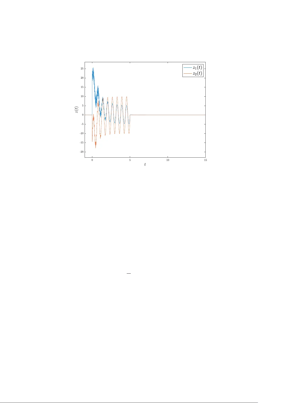
Dissipativ e Stabilization of Linear Systems wit h Time- V ar ying General Distr ibuted Dela ys (Com plete V ersion) ⋆ Qian Feng a, ∗ , Sing Kiong Nguang b , Wilfrid P err uquetti a a École Centrale de Lille, CRIS tAL, UMR CNRS 9189 Cit e Scientiﬁque, 59651, V illneuve d’ascq Cedex, F r ance b Department of Electrical and Comput er Engineering, The Univ ersity of Auc kland, Auc kland 1010, New Zealand Abstract Ne w met hods are dev eloped for the stabilization of a linear system wit h gener al time-varying distributed dela ys existing at the system’ s states, inputs and outputs. In contrast to most existing literature where the function of time-varying dela y is continuous and bounded, w e assume it to be bounded and measurable. Furthermore, t he distributed dela y kernels can be an y square-integrable function ov er a bounded inter val, where the kernels are handled directly b y using a decomposition scenario without using appro ximations. By constructing a Krasov ski functional via t he application of a no v el integ ral inequality , suﬃcient conditions for the existence of a dissipativ e state feedback controller are deriv ed in terms of matrix inequalities without utilizing the existing reciprocally con v ex combination lemmas. The proposed synthesis (stability) conditions, which take dissipativity into account, can be either solv ed directly by a standard numerical solv er of semideﬁnite programming if they are con v ex, or reshaped into linear matrix inequalities, or solv ed via a proposed iterativ e algorit hm. T o the best of our know ledge, no existing methods can handle t he synthesis problem inv estig ated in this paper . Finall y , numerical examples are presented to demonstrate t he eﬀectiv eness of the proposed methodologies. Keywords: Dissipativ e Systems; Dis tributed T ime- V arying Dela ys; Integ ral Inequality ; Controller Synthesis 1. Introduction Time dela ys exist in systems aﬀected b y transportation and af tereﬀects Richard (2003). For certain real-time application such as the models in Anthonis et al. (2007); Molnár & Insperger (2015), dela ys can be time-v arying. It is of great research interest to in ves tigate a sys tem with bounded time-varying dela ys since it can be applied in modeling sam pled-data Fridman et al. (2004) or networ ked control systems (NCSs) Hespanha et al. (2007). One can ﬁnd many existing results in the literature pertaining to t he stability analysis Jiang (2006); Seuret et al. (2013); Kw on et al. (2016); Qian et al. (2018) and s tabilization Jiang (2005); F ridman (2006); Mohajerpoor et al. (2018) of linear time-v arying dela y systems wit h a bounded continuous time- v arying delay . The methods in t he aforementioned references are based on the cons truction of Krasov ski functionals (KF) Briat (2014), where the time-varying dela y is embedded only in x ( t − r ( t )) . It has been ⋆ This w ork was partially supported by the ANR (Ag ence nationale de la recherche) Project Finite4SoS (ANR -15-CE23-0007). ∗ Corresponding author Email addresses: qfen204@aucklanduni.ac.nz, qian.feng@centralelille.fr (Qian Feng), sk.nguang@auckland.ac.nz (Sing Kiong Nguang), wilfrid.perruquetti@centralelille.fr (Wilfrid Perruquetti) This paper is the complete ver sion of the paper https://doi.or g/10.1016/j.automatica.2020.109227 published by A utomatica. shown in Gao et al. (2008, 2010) t hat the KF method for linear systems wit h x ( t − r ( t )) can be utilized to solv e synthesis problems of NCSs. It is w orthy mention that unlike systems with constant dela ys, frequency- domain-based approaches Breda et al. (2005); Michiels & Niculescu (2014); Gehring et al. (2014); V yhlídal & Zítek (2014) ma y not be usable to analyze the spectrum of a system if t he exact expression of r ( t ) is unknown. It has been pointed out in Goebel et al. (2011) t hat the digital communication channel of N CSs with stochas tic packet dela ys and loss can be modeled b y distributed dela ys. Moreov er , the results in Y an et al. (2019) hav e shown that a netw ork ed control system wit h a netw ork channel dela y stabilized by an ev ent- triggered H ∞ controller can be modeled as a distributed dela y system, where t he dela y is of constant values. T o the best of our kno wledg e how ev er , no existing methods can handle the stabilization problem of systems with general distributed delays where the dela y function is time-v ar ying and unknown. In Theorem 2 of Zhou et al. (2012), a method of stabilizing systems in t he form of ˙ x ( t ) = A x ( t ) + R 0 − r ( t ) B ( τ ) u ( t + τ ) d τ is proposed. N ev ert heless, all the poles of A in Zhou et al. (2012) are assumed to be located on the imaginar y axis, and t he low er bound of r ( t ) is restricted to 0 < r ( t ) ≤ r 2 . The stability of positiv e linear systems with distributed time-varying delays is in v estigated in Ngoc (2013); Cui et al. (2018). Although the method in Ngoc (2013) does include criteria to determine the stability of non-positiv e linear systems, t he structure of the dela y function r ( · ) ∈ C ( R ≥ 0 # (0 , r 2 ]) t herein is still restrictiv e. On the o ther hand, the synthesis (stability analysis) methods proposed in Münz et al. (2009); Goebel et al. (2011); Gouaisbaut et al. (2015); Seuret et al. (2015); Feng & Nguang (2016), which are dev eloped to handle linear distributed dela y systems wit h constant dela y v alues, ma y not be easil y extended to cope with systems wit h an unknown time-varying dela y . This is especially true for the approximation approaches in Münz et al. (2009); Goebel et al. (2011); Gouaisbaut et al. (2015); Seuret et al. (2015), since t he appro ximation coeﬃcients can become nonlinear wit h respect to r ( t ) if t he distributed dela y ker nels are approximated o v er [ − r ( t ) , 0] . Consequently , it is obvious that new met hods should be dev eloped f or t he s tabilization (stability anal ysis) of linear sys tems with general distributed time-v ar ying dela ys. In t his paper , ne w met hods f or t he stabilization of a linear system wit h general distributed time-v arying dela ys are dev eloped based on t he construction of a g eneral Kraso vski functional, where the time-v arying dela y function r ( · ) is unknown but measurable and bounded b y giv en values 0 ≤ r 1 ≤ r 2 , r 2 > 0 . Our system contains distributed dela ys at t he system’ s states, inputs and outputs, where the dela y kernels can be any L 2 function ov er a giv en interv al. T o ensure that t he proposed methods are deno ted by linear matrix inequalities (LMIs) wit h ﬁnite-dimensions, a nov el integ ral inequality is proposed where t he symmetric matrix of the inequality’s low er bound is not a function of r ( t ) but r 1 and r 2 . By using this inequality in constructing a general KF , suﬃcient conditions for the existence of a state feedback controller , which ensure t hat t he system is stable and dissipative wit h a supply function, are deriv ed in terms of matrix inequalities summarized in the ﬁrst theorem of t his paper . The synthesis condition of the ﬁrs t theorem has a bilinear matrix inequality (BMI) if a stabilization problem is considered, whereas it becomes con v ex if non-stabilization scenarios are concerned. T o circum v ent the diﬃculties of solving non-conv ex conditions, a second theorem deno ted by LMIs is proposed via the application of Projection Lemma Gahinet & Apkarian (1994). Next, an iterativ e algorit hm, based on the inner con v ex appro ximation scheme dev eloped in Dinh et al. (2012), is proposed for solving t he BMI in the ﬁrst t heorem, where t he algorithm can be initiated b y a feasible solution of the second theorem. T o the best of our know ledge, no existing methods in the 2 peer -review ed literature can handle the synt hesis problem in this paper . Finall y , tw o numerical examples are presented to demonstr ate the eﬀectiv eness of our proposed met hodologies. The major contributions of this paper are summarized as follo ws: • W e believ e t he dissipative synthesis problem inv estigated in this paper cannot be dealt with by any existing met hod. Our model is suﬃciently general wit h respect to g enerality of r ( t ) and distributed dela y kernels. A bounded and measurable dela y function can be particularl y useful to model dis- continuous time-varying dela ys. Finall y , the proposed methods only require the use of standard algorithms for semideﬁnite programming (SDP) without asking for nonlinear solv ers. • The handling of distributed dela y kernels in this paper , which is based on t he application of a decomposition approach, allows one to consider any L 2 function ov er an interv al, ev en the interval is related to r ( t ) . This av oids the use of any form of appro ximations so that no nonlinear terms of r ( t ) will be introduced into the proposed synthesis conditions. • The proposed integral inequality allows one to construct Kraso vski functionals without utilizing the reciprocally -conv ex-combination type of lemmas Par k et al. (2011); Seuret & Gouaisbaut (2017); Zhang et al. (2017a,b); Seuret et al. (2018) which ma y not be capable of pro viding tr actable solutions to the problem considered in this paper . The rest of the paper is outlined as follo ws. The synthesis problem inv estigated in t his paper is ﬁrst formulated in Section 2 where w e explain t he principle of the decomposition approach. Next, the main results on dissipative stabilization are presented in Section 3, which are summarized in Theorem 1 and 2 and Algorithm 1. Finall y , numerical examples and their simulation results are presented in Section 4 prior to the ﬁnal conclusion. Notation Let Y X = { f ( · ) : f ( · ) is a function from X onto Y } and R ≥ a = { x ∈ R : x ≥ a } and S n = { X ∈ R n × n : X = X ⊤ } . C ( X # R n ) := n f ( · ) ∈ ( R n ) X : f ( · ) is continuous on X o and C k ([ a, b ] # R n ) := n f ( · ) ∈ C ([ a, b ] # R n ) : d k f ( x ) d x k ∈ C ([ a, b ] # R n ) o where t he deriv ativ es at a and b are one-sided. Moreo ver , M L ( X ) / B ( R )  X # R  :=  f ( · ) ∈ X R : ∀Y ∈ B ( R ) , f − 1 ( Y ) ∈ L ( X )  denotes the space of all L ( X ) / B ( R ) measurable functions from X onto R , where L ( X ) contains all the subsets of X which are Lebesgue mea- surable, and B ( R ) is t he Borel σ –algebr a on R . Note that w e frequently abbreviate M L ( X ) / B ( R )  X # R  as M ( X # R ) when t he context is clear . In addition, w e deﬁne L p ( X # R n ) =  f ( · ) ∈ M L ( X ) / B ( R n )  X # R n  : k f ( · ) k p < + ∞  with the semi-norm k f ( · ) k p :=  R X k f ( x ) k p 2 d x  1 p where X ⊆ R n . Moreov er , w e use e ∀ x ∈ X to denote the meaning of for almost all x ∈ X with respect to the Lebesgue measure. Sy ( X ) := X + X ⊤ stands for the sum of a matrix wit h its transpose. W e use Col n i =1 x i :=  Ro w n i =1 x ⊤ i  ⊤ =  x ⊤ 1 · · · x ⊤ i · · · x ⊤ n  ⊤ to denote a column v ector containing a sequence of mat hematical objects (scalars, v ectors, matrices etc.). The symbol ∗ is used to indicate [ ∗ ] Y X = X ⊤ Y X or X ⊤ Y [ ∗ ] = X ⊤ Y X or [ A B ∗ C ] =  A B B ⊤ C  . O n,m denotes a n × m zero matrix which can be abbreviated b y O n if n = m, while 0 n represents a n × 1 column vect or . W e frequentl y use X ⊕ Y =  X O ∗ Y  to denote the diagonal sum of tw o matrices. ⊗ stands for the Kroneck er product. The order of matrix operations is matrix (scalars) multiplications > ⊗ > ⊕ > + t hroughout the paper . Finall y , em pty matrices [ ] 0 ,m , [ ] m, 0 , [ ] 0 , 0 (St oer & Witzgall, 1970, See I.7) with m ∈ N , which follo w 3 the same deﬁnition and prog ramming rules in Matlab © , are applied in t his paper to render our synthesis conditions capable of handling the case of r 1 = 0 ; r 2 > 0 or r 1 = r 2 . N ote that w e deﬁne Col n i =1 x i = [ ] 0 ,m if n < 1 , where [ ] 0 ,m is an emp ty matrix with an appropriate column dimension m ∈ N based on speciﬁc contexts. 2. Problem formulation Consider a linear distributed dela y system ˙ x ( t ) = A 1 x ( t ) + Z 0 − r ( t ) e A 2 ( τ ) x ( t + τ ) d τ + B 1 u ( t ) + Z 0 − r ( t ) e B 2 ( τ ) u ( t + τ ) d τ + D 1 w ( t ) , e ∀ t ≥ t 0 z ( t ) = C 1 x ( t ) + Z 0 − r ( t ) e C 2 ( τ ) x ( t + τ ) d τ + B 4 u ( t ) + Z 0 − r ( t ) e B 5 ( τ ) u ( t + τ ) d τ + D 2 w ( t ) , ∀ θ ∈ [ − r 2 , 0] , x ( t 0 + θ ) = ϕ ( τ ) , r ( · ) ∈ M ( R # [ r 1 , r 2 ]) (1) to be stabilized, where t 0 ∈ R and ϕ ( · ) ∈ C ([ − r 2 , 0] # R n ) , and r 2 > 0 , r 2 ≥ r 1 ≥ 0 are giv en constants. Furthermore, x : [ t 0 − r 2 , ∞ ) → R n satisﬁes (1), u ( t ) ∈ R p denotes in put signals, w ( t ) ∈ L 2 ([ t 0 , + ∞ ) # R q ) represents disturbance, and z ( t ) ∈ R m is t he regulated output. The size of t he giv en s tate space parameters in (1) is determined by t he values of n ∈ N and m ; p ; q ∈ N 0 := N ∪ { 0 } . Finall y , the matrix-valued distributed dela ys in (1) satisfy e A 2 ( · ) ∈ L 2 ([ − r 2 , 0] # R n × n ) , e C 2 ( · ) ∈ L 2 ([ − r 2 , 0] # R m × n ) e B 2 ( · ) ∈ L 2 ([ − r 2 , 0] # R n × p ) , e B 5 ( · ) ∈ L 2 ([ − r 2 , 0] # R m × p ) . (2) Remark 1. Systems with distributed dela ys and a time-varying delay function can be found among the models of neural netw orks Ge et al. (2019); Dong et al. (2019). The distributed dela ys in (2) are inﬁnite-dimensional. In order to construct synthesis cons traints with ﬁnite dimensions for (1), w e propose a decomposition scenario as follo ws. Proposition 1. The conditions in (2) holds if and onl y if ther e exis t f 1 ( · ) ∈ C 1 ([ − r 2 , 0] # R d 1 ) , f 2 ( · ) ∈ C 1 ([ − r 2 , 0] # R d 2 ) , φ 1 ( · ) ∈ L 2 ([ − r 2 , 0] # R δ 1 ) , φ 2 ( · ) ∈ L 2 ([ − r 2 , 0] # R δ 2 ) , M 1 ∈ R d 1 × κ 1 , M 2 ∈ R d 2 × κ 2 , A 2 ∈ R n × κ 1 n , A 3 ∈ R n × κ 2 n , B 2 ∈ R n × κ 1 p , B 3 ∈ R n × κ 2 p , C 2 ∈ R m × κ 1 n , C 3 ∈ R m × κ 2 n , B 5 ∈ R m × κ 1 p and B 6 ∈ R m × κ 2 p such that ∀ τ ∈ [ − r 1 , 0] , e A 2 ( τ ) = A 2  b f 1 ( τ ) ⊗ I n  , e B 2 ( τ ) = B 2  b f 1 ( τ ) ⊗ I p  , (3) ∀ τ ∈ [ − r 2 , − r 1 ] , e A 2 ( τ ) = A 3  b f 2 ( τ ) ⊗ I n  , e B 2 ( τ ) = B 3  b f 2 ( τ ) ⊗ I p  , (4) ∀ τ ∈ [ − r 1 , 0] , e C 2 ( τ ) = C 2  b f 1 ( τ ) ⊗ I n  , e B 5 ( τ ) = B 5  b f 1 ( τ ) ⊗ I p  , (5) ∀ τ ∈ [ − r 2 , − r 1 ] , e C 2 ( τ ) = C 3  b f 2 ( τ ) ⊗ I n  , e B 5 ( τ ) = B 6  b f 2 ( τ ) ⊗ I p  , (6) ∀ τ ∈ [ − r 2 , 0] , d f 1 ( τ ) d τ = M 1 b f 1 ( τ ) , d f 2 ( τ ) d τ = M 2 b f 2 ( τ ) (7) G 1 = [ ] 0 × 0 or G 1  0 , G 1 := Z 0 − r 1 b f 1 ( τ ) b f ⊤ 1 ( τ ) d τ (8) G 2 = [ ] 0 × 0 or G 2  0 , G 2 := Z − r 1 − r 2 b f 2 ( τ ) b f ⊤ 2 ( τ ) d τ (9) 4 where κ 1 = d 1 + δ 1 , κ 2 = d 2 + δ 2 with d 1 ; d 2 ; δ 1 ; δ 2 ∈ N 0 satisfying d 1 + d 2 > 0 , and b f 1 ( τ ) =  φ 1 ( τ ) f 1 ( τ )  , b f 2 ( τ ) =  φ 2 ( τ ) f 2 ( τ )  . (10) F inally , the derivatives in (7) at τ = 0 and τ = − r 2 are one-sided derivatives. Not e t hat if matrix multiplications in (3) – (10) inv ol ve an y empty matrix, t hen it follows t he deﬁnition and pr operties of empty matrices in Matlab. Proof. First of all, it is str aightforwar d to see that (2) is implied by (3)–(10) since φ 1 ( · ) ∈ L 2 ([ − r 2 , 0] # R δ 1 ) , φ 2 ( · ) ∈ L 2 ([ − r 2 , 0] # R δ 2 ) , f 1 ( · ) ∈ C 1 ([ − r 2 , 0] # R d 1 ) ⊂ L 2 ([ − r 2 , 0] # R d 1 ) and f 2 ( · ) ∈ C 1 ([ − r 2 , 0] # R d 2 ) ⊂ L 2 ([ − r 2 , 0] # R d 2 ) . N ow we start to prov e (2) implies the existence of the parameters in Proposition 1 satisfying (3)– (9). Giv en an y f 1 ( · ) ∈ C 1 ([ − r 2 , 0] # R d 1 ) , f 2 ( · ) ∈ C 1 ([ − r 2 , 0] # R d 2 ) , one can alw a ys ﬁnd appropriate φ 1 ( · ) ∈ L 2 ([ − r 2 , 0] # R δ 1 ) , φ 2 ( · ) ∈ L 2 ([ − r 2 , 0] # R δ 2 ) with M 1 ∈ R d 1 × κ 1 and M 2 ∈ R d 2 × κ 2 such that (7)–(9) are satisﬁed with (10), where G 1  0 and G 2  0 in (8) infers t hat the functions in b f 1 ( · ) and b f 2 ( · ) in (10) are linearl y independent 1 in a Lebesgue sense o ver [ − r 2 , 0] and [ − r 2 , − r 1 ] , respectiv ely . This is tr ue since d f 1 ( τ ) d τ ( · ) ∈ L 2 ([ − r 1 , 0] # R d 1 ) and d f 1 ( τ ) d τ ( · ) ∈ L 2 ([ − r 2 , − r 2 ] # R d 2 ) , and t he dimensions of φ 1 ( τ ) and φ 2 ( τ ) can be arbitraril y enlarged with more linearl y independent functions. N ote that if any vect or-v alued function f 1 ( τ ) , f 2 ( τ ) , φ 1 ( τ ) and φ 2 ( τ ) is [ ] 0 × 1 , then it can be handled b y the application of emp ty matrices as reﬂected in (8) and (9). Giv en an y f 1 ( · ) ∈ C 1 ([ − r 2 , 0] # R d 1 ) , f 2 ( · ) ∈ C 1 ([ − r 2 , 0] # R d 2 ) , we hav e sho wn t hat one can alw a ys construct appropriate φ 1 ( · ) ∈ L 2 ([ − r 2 , 0] # R δ 1 ) , φ 2 ( · ) ∈ L 2 ([ − r 2 , 0] # R δ 2 ) with M 1 and M 2 such t hat the conditions in (7)–(9) are satisﬁed wit h (10). As a result, based on the deﬁnition of matrix-valued functions and t he fact that t he dimensions of φ 1 ( τ ) and φ 2 ( τ ) can be arbitraril y increased, one can alw a ys construct appropriate constant matrices A 2 ,i , A 3 ,i , C 2 ,i , C 3 ,i , B 2 ,i , B 3 ,i , B 5 ,i , B 6 ,i and f 1 ( τ ) , f 2 ( τ ) , φ 1 ( τ ) and φ 2 ( τ ) such that ∀ τ ∈ [ − r 1 , 0] , e A 2 ( τ ) = κ 1 X i =1 A 2 ,i g i ( τ ) , e C 2 ( τ ) = κ 1 X i =1 C 2 ,i g i ( τ ) , (11) ∀ τ ∈ [ − r 1 , 0] , e B 2 ( τ ) = κ 1 X i =1 B 2 ,i g i ( τ ) , e B 5 ( τ ) = κ 1 X i =1 B 5 ,i g i ( τ ) (12) ∀ τ ∈ [ − r 2 , − r 1 ] , e A 2 ( τ ) = κ 2 X i =1 A 3 ,i h i ( τ ) , e C 2 ( τ ) = κ 2 X i =1 C 3 ,i h i ( τ ) , (13) ∀ τ ∈ [ − r 2 , − r 1 ] , e B 2 ( τ ) = κ 2 X i =1 B 3 ,i h i ( τ ) , e B 5 ( τ ) = κ 2 X i =1 B 6 ,i h i ( τ ) (14) g ⊤ ( τ ) = b f ⊤ 1 ( τ ) =  φ ⊤ 1 ( τ ) f ⊤ 1 ( τ )  ⊤ , h ( τ ) = b f ⊤ 2 ( τ ) =  φ ⊤ 2 ( τ ) f ⊤ 2 ( τ )  ⊤ (15) with κ 1 ; κ 2 ∈ N 0 , where f 1 ( τ ) , f 2 ( τ ) , φ 1 ( τ ) and φ 2 ( τ ) satisfy (7)–(9) for some M 1 and M 2 . No w (11)–(14) can be further rewritten as ∀ τ ∈ [ − r 1 , 0] , e A 2 ( τ ) =  κ 1 Ro w i =1 A 2 ,i   b f 1 ( τ ) ⊗ I n  , e C 2 ( τ ) =  κ 1 Ro w i =1 C 2 ,i   b f 1 ( τ ) ⊗ I n  ∀ τ ∈ [ − r 2 , − r 1 ] , e A 2 ( τ ) =  κ 2 Ro w i =1 A 3 ,i   b f 2 ( τ ) ⊗ I n  , e C 2 ( τ ) =  κ 2 Ro w i =1 C 3 ,i   b f 2 ( τ ) ⊗ I n  ∀ τ ∈ [ − r 1 , 0] , e B 2 ( τ ) =  κ 1 Ro w i =1 B 2 ,i   b f 1 ( τ ) ⊗ I p  , e B 5 ( τ ) =  κ 1 Ro w i =1 B 5 ,i   b f 1 ( τ ) ⊗ I p  ∀ τ ∈ [ − r 2 , − r 1 ] , e B 2 ( τ ) =  κ 2 Ro w i =1 B 3 ,i   b f 2 ( τ ) ⊗ I p  , e B 5 ( τ ) =  κ 2 Ro w i =1 B 6 ,i   b f 2 ( τ ) ⊗ I p  . (16) 1 See Theorem 7.2.10 in Horn & Johnson (2012) for more information 5 which are in line with the forms in (3)–(6). Giv en all t he aforementioned statements w e ha ve presented, then Proposition 1 is prov ed. ■ Remark 2. Proposition 1 provides an eﬀectiv e wa y to handle the distributed dela ys in (1). It uses a group of basis functions to decompose the distributed dela ys without appealing to t he application of approximations. The potential choices of the functions in (3)–(6) will be further discussed in the next section in light of the construction of a KF related to f 1 ( · ) and f 2 ( · ) . 2.1. The formulation of t he closed-loop sys tem In this paper , w e want to construct a state feedback controller u ( t ) = K x ( t ) with K ∈ R p × n to stabilize the open-loop system in (1). Then the corresponding closed-loop system is denoted as ˙ x ( t ) = A 1 x ( t ) + Z 0 − r 1 A 2  b f 1 ( τ ) ⊗ I n  x ( t + τ ) d τ + Z − r 1 − r ( t ) A 3  b f 2 ( τ ) ⊗ I n  x ( t + τ ) d τ + B 1 K x ( t ) + Z 0 − r 1 B 2 ( I κ 1 ⊗ K )  b f 1 ( τ ) ⊗ I n  x ( t + τ ) d τ + Z − r 1 − r ( t ) B 3 ( I κ 2 ⊗ K )  b f 2 ( τ ) ⊗ I n  x ( t + τ ) d τ + D 1 w ( t ) z ( t ) = C 1 x ( t ) + Z 0 − r 1 C 2  b f 1 ( τ ) ⊗ I n  x ( t + τ ) d τ + Z − r 1 − r ( t ) C 3  b f 2 ( τ ) ⊗ I n  x ( t + τ ) d τ + B 4 K x ( t ) + Z 0 − r 1 B 5 ( I κ 1 ⊗ K )  b f 1 ( τ ) ⊗ I n  x ( t + τ ) d τ + Z − r 1 − r ( t ) B 6 ( I κ 2 ⊗ K )  b f 2 ( τ ) ⊗ I n  x ( t + τ ) d τ + D 2 w ( t ) , ∀ θ ∈ [ − r 2 , 0] , x ( t 0 + θ ) = ϕ ( τ ) , r ( · ) ∈ M ( R # [ r 1 , r 2 ]) (17) b y Lemma 2 and Proposition 1, where t he decom position of the distributed dela ys are constructed via  b f i ( τ ) ⊗ I p  K =  b f i ( τ ) ⊗ I p  (1 ⊗ K ) =  I κ i b f i ( τ ) ⊗ K I n  = ( I κ i ⊗ K )  b f i ( τ ) ⊗ I n  , i = 1 , 2 (18) b y (A.2). N ote that (17) has diﬀerent forms for the following three cases r 2 > r 1 > 0 , and r 1 = 0 ; r 2 > 0 , and r 1 = r 2 > 0 . 2 This implies that each case of t hese t hree ma y require a distinct formulation for t he corresponding synthesis conditions for (17). T o a v oid deriving t hree separated synthesis conditions, w e rewrite (17) as ˙ x ( t ) =  A + B 1  I b 3+ κ ⊗ K  ⊕ O q   χ ( t ) , e ∀ t ≥ t 0 z ( t ) =  C + B 2  I b 3+ κ ⊗ K  ⊕ O q  χ ( t ) , ∀ θ ∈ [ − r 2 , 0] , x ( t 0 + θ ) = ϕ ( θ ) (19) with t 0 and ϕ ( · ) in (1), where κ = κ 1 + 2 κ 2 and A = h b O n,n A 1 A 2  √ G 1 ⊗ I n  A 3  √ G 2 ⊗ I n  O n,κ 2 n D 1 i (20) B 1 = h b O n,p B 1 B 2  √ G 1 ⊗ I p  B 3  √ G 2 ⊗ I p  O n,κ 2 p O n,q i (21) C = h b O m,n C 1 C 2  √ G 1 ⊗ I n  C 3  √ G 2 ⊗ I n  O m,κ 2 n D 2 i (22) B 2 = h b O m,p B 4 B 5  √ G 1 ⊗ I p  B 6  √ G 2 ⊗ I p  O m,κ 2 p O m,q i (23) 2 Since (17) becomes a dela y-free system with r 1 = r 2 = 0 , hence such a case is not considered here. 6 χ ( t ) =                   b 1 x ( t − r 1 ) 1 x ( t − r 2 ) x ( t ) R 0 − r 1  q G − 1 1 b f 1 ( τ ) ⊗ I n  x ( t + τ ) d τ R − r 1 − r ( t )  q G − 1 2 b f 2 ( τ ) ⊗ I n  x ( t + τ ) d τ R − r ( t ) − r 2  q G − 1 2 b f 2 ( τ ) ⊗ I n  x ( t + τ ) d τ w ( t )                   , b O n,p =        O n, 2 p for r 2 > r 1 > 0 O n,p for r 1 = r 2 > 0 O n,p for r 1 = 0; r 2 > 0 b 3 =        3 for r 2 > r 1 > 0 2 for r 1 = r 2 > 0 2 for r 1 = 0; r 2 > 0 (24) 1 = ( I n for r 2 > r 1 ≥ 0 [ ] 0 × n for r 1 = r 2 > 0 , b 1 = ( I n for r 2 ≥ r 1 > 0 [ ] 0 × n for r 1 = 0; r 2 > 0 . (25) N ote t hat √ X stands for t he unique square roo t of X  0 and the ter ms in (20)–(23) are obtained b y the follo wing relations for i ∈ { 1 , 2 } :  b f i ( τ ) ⊗ I n  = p G i q G − 1 i b f i ( τ ) ⊗ I n =  p G i ⊗ I n   q G − 1 i b f i ( τ ) ⊗ I n  , (26) ( I κ i ⊗ K )  b f i ( τ ) ⊗ I n  =  p G i q G − 1 i ⊗ K   b f i ( τ ) ⊗ I n  =  p G i ⊗ I p  ( I κ i ⊗ K )  q G − 1 i b f i ( τ ) ⊗ I n  (27) which themselv es can be obtained via (A.1) with the fact t hat G 1 and G 2 in (8) are inv ertible 3 . No w the expressions of the closed-loop system in (17) at r 1 = r 2 > 0 and r 1 = 0 ; r 2 > 0 can be obtained b y (19) with r 1 = r 2 > 0 , d 2 = δ 2 = 0 , and r 1 = 0 ; r 2 > 0 , d 1 = δ 1 = 0 in (20)–(24), respectiv ely . By introducing the terms b O , b 3 , 1 and b 1 in ( 24)–(25), the closed-loop system in (17) can be equivalentl y denoted by the form in (19) which can characterize all the cases of r 2 ≥ r 1 ≥ 0 , r 2 > 0 wit hout introducing redundant terms into the parameters in (20)–(24). This is critical in deriving w ell-posed synthesis conditions in t his paper . 3 No te that √ X − 1 =  √ X  − 1 for an y X ≻ 0 , based on t he application of the eigendecomposition of X ≻ 0 7 Remark 3. The existence and uniqueness of the solution of the closed-loop system (19) are guaran- teed b y Theorem 1.1 in Chap ter 6 of Hale & L unel (1993) which is dev eloped for a gener al linear TDS. Speciﬁcall y , consider R 0 − r ( t ) G ( τ ) ϕ ( τ ) d τ wit h r ( · ) ∈ M  R # [ r 1 , r 2 ]  , r 2 > 0 , r 2 ≥ r 1 ≥ 0 and G ( · ) ∈ L 2 ([ − r 2 , 0] # R m × n ) and ϕ ( · ) ∈ C ([ − r 2 , 0] # R n ) . By using the Cauch y Schw artz inequality with the fact that G ( · ) ∈ L 2 ([ − r 2 , 0] # R m × n ) and ϕ ( · ) ∈ C ([ − r 2 , 0] # R n ) ⊂ L 2 ([ − r 2 , 0] # R n ) , we ha v e      Z 0 − r ( t ) G ( τ ) ϕ ( τ ) d τ      2 =      Z 0 − r ( t ) m Col i =1 g ⊤ i ( τ ) ϕ ( τ ) d τ      2 = v u u t m X i =1 Z 0 − r ( t ) g ⊤ i ( τ ) ϕ ( τ ) d τ ! 2 ≤ v u u t m X i =1 Z 0 − r ( t ) k g i ( τ ) k 2 2 d τ Z 0 − r ( t ) k ϕ ( τ ) k 2 2 d τ ! ≤ v u u t m X i =1  Z 0 − r 2 k g i ( τ ) k 2 2 d τ Z 0 − r 2 k ϕ ( τ ) k 2 2 d τ  ≤ v u u t m X i =1  α Z 0 − r 2 k ϕ ( · ) k 2 ∞ d τ  = q mr 2 α k ϕ ( · ) k 2 ∞ = √ mr 2 α k ϕ ( · ) k ∞ (28) for some α > 0 , where G ( τ ) = Col m i =1 g ⊤ i ( τ ) . No w this shows that all the integrals in (19) satisfy the inequality belo w eq.(1.5) in Chapter 6 of Hale & L unel (1993). This is because R 0 − r ( t ) G ( τ ) ϕ ( τ ) d τ = R 0 − r 2 u ( r ( t ) + τ ) G ( τ ) ϕ ( τ ) d τ that t he function u ( r ( t ) + τ ) G ( τ ) is integrable in τ f or all t ∈ R and measurable in t ∈ R for all τ ∈ [ − r 2 , 0] . 3. Main results Since t he diﬀerential equation in (17) holds for almos t all t ≥ t 0 ev en in the case of w ( t ) ≡ 0 n , t hus t he standar d L yapuno v Kraso vski s tability theorem 4 cannot be applied to (17). A L yapuno v -Kraso vski s tability criterion is presented as follow s which can anal yze t he stability of (17). See Lemma 4 in Appendix A for the gener al L y apunov -Kraso vski s tability criterion which is deriv ed for analyzing the stability of general functional diﬀerential equations subject to the Caratheodory conditions in section 2.6 of Hale & Lunel (1993). Corollar y 1. Let w ( t ) ≡ 0 q in (19) and r 2 ≥ r 1 ≥ 0 , r 2 > 0 be given, then t he trivial solution x ( t ) ≡ 0 n of (19) is uniforml y asymp to tically st able in C ([ − r 2 , 0] # R n ) if ther e exist ϵ 1 ; ϵ 2 ; ϵ 3 > 0 and a diﬀerentiable functional v : C ([ − r 2 , 0] # R n ) → R with v ( 0 n ( · )) = 0 such that ∀ ϕ ( · ) ∈ C ([ − r 2 , 0] # R n ) , ϵ 1 k ϕ (0) k 2 2 ≤ v ( ϕ ( · )) ≤ ϵ 2 k ϕ ( · ) k 2 ∞ , (29) e ∀ t ≥ t 0 ∈ R , d d t v ( x t ( · )) ≤ − ϵ 3 k x ( t ) k 2 2 (30) where x t ( · ) in (30) is deﬁned by the equality ∀ t ≥ t 0 , ∀ θ ∈ [ − r 2 , 0] , x t ( θ ) = x ( t + θ ) in which x ( · ) ∈ C ( R ≥ t 0 − r 2 # R n ) satisﬁes ˙ x ( t ) =  A + B 1  I b 3+ κ ⊗ K  ⊕ O q   χ ( t ) in (19) with w ( t ) ≡ 0 q . Proof. Since (19) wit h w ( t ) ≡ 0 q is a linear system and r ( · ) ∈ M ( R # [ r 1 , r 2 ]) , thus (19) with w ( t ) ≡ 0 q is a special case of t he g eneral time-v ar ying system in (A.5). Then (29) and (30) can be obtained b y letting α 1 ( s ) = ϵ 1 s 2 , α 2 ( s ) = ϵ 2 s 2 , α 3 ( s ) = ϵ 3 s 2 with ϵ 1 ; ϵ 2 ; ϵ 3 > 0 . ■ 4 See Theorem 2.1 of Section 5.1 in Hale & L unel (1993), and Theorem 1.3 in Gu et al. (2003) 8 Deﬁnition 1. Giv en 0 6 = r 2 ≥ r 1 ≥ 0 , the closed-loop system in (19) with a supply rate function s ( z ( t ) , w ( t )) is said to be dissipativ e if t here exists a diﬀerentiable functional v : C ([ − r 2 , 0] # R n ) → R such t hat e ∀ t ≥ t 0 , ˙ v ( x t ( · )) − s ( z ( t ) , w ( t )) ≤ 0 (31) where t 0 , z ( t ) and w ( t ) are giv en in (19) together wit h ∀ t ≥ t 0 , ∀ θ ∈ [ − r 2 , 0] , x t ( θ ) = x ( t + θ ) where x ( t ) is the solution of t he system in (19). N ote that (31) implies t he origin integral-based deﬁnition of dissipativity via the properties of Lebesgue integrals. T o characterize dissipativity , a quadratic suppl y function s ( z ( t ) , w ( t )) = " z ( t ) w ( t ) # ⊤ " e J ⊤ J − 1 1 e J J 2 ∗ J 3 # " z ( t ) w ( t ) # , S m 3 e J ⊤ J − 1 1 e J  0 , S m 3 J − 1 1 ≺ 0 , e J ∈ R m × m (32) is applied in this paper where the structure of (32) is based t he g eneral quadratic constr aints in v estigated in Scherer et al. (1997) tog et her with the idea of fact orizing the matrix U j in Scherer et al. (1997). N ote t hat the supply rate function in (32) can char acterize numerous performance criteria such as • L 2 gain perf ormance: J 1 = − γ I m , e J = I m , J 2 = O m,q , J 3 = γ I q where γ > 0 . • P assivity: J 1 ∈ S m ≺ 0 , e J = O m , J 2 = I m , J 3 = O m with m = q . T wo integ ral inequalities, which are presented in Lemma 5 and 6 in 5, are required to deriv e t he main results in t his paper . The second inequality in Lemma 6 is speciﬁcally proposed as an important contribution in this paper to ensure that the dimensions of the resulting synt hesis conditions are ﬁnite. The main results of this paper are summarized in tw o theorems and an algorit hm in the rest of t his section. Theorem 1. Let r 2 > r 1 > 0 and all the par ameters in Proposition 1 be given, then the closed-loop sys tem (19) with t he supply r ate function in (32) is dissipative and the trivial solution x ( t ) ≡ 0 n of (19) wit h w ( t ) ≡ 0 q is uniforml y asymp to tically s table in C ([ − r, 0] # R n ) if t here exis t K ∈ R p × n and P 1 ∈ S n , P 2 ∈ R n × ϱ , P 3 ∈ S ϱ with ϱ = ( d 1 + d 2 ) n and Q 1 ; Q 2 ; R 1 ; R 2 ∈ S n and Y ∈ R n × n such t hat  P 1 P 2 ∗ P 3  +  O n ⊕  I d 1 ⊗ Q 1  ⊕  I d 2 ⊗ Q 2   0 , (33) Q 1  0 , Q 2  0 , R 1  0 ,  R 2 Y ∗ R 2   0 , (34)  Ψ Σ ⊤ e J ⊤ ∗ J 1  = Sy  P ⊤ Π  + Φ ≺ 0 (35) where Σ = C + B 2  I b 3+ κ ⊗ K  ⊕ O q  with C and B 2 in (22) and (23) , and Ψ = Sy           b O ⊤ n,n b O ⊤ ϱ,n I n O n,ϱ O κn,n b I ⊤ O q ,n O q ,ϱ       P 1 P 2 ∗ P 3  " A + B 1  I b 3+ κ ⊗ K  ⊕ O q  h b F ⊗ I n O ϱ,q i # −    b O ⊤ m,n O ( n + κn ) ,m J ⊤ 2    Σ      − Ξ (36) b I =  q F − 1 1 ⊕ q F − 1 2   O d 1 ,δ 1 I d 1 O d 1 ,δ 2 O d 1 ,d 2 O d 1 ,δ 2 O d 1 ,d 2 O d 2 ,δ 1 O d 2 ,d 1 O d 2 ,δ 2 I d 2 O d 2 ,δ 2 I d 2   √ G 1 ⊕ √ G 2 ⊕ √ G 2  ⊗ I n (37) 9 Ξ = " [ Q 1 − Q 2 − r 3 R 2 ] ⊕ [ 1 Q 2 ] ⊕ h b 1 ( − Q 1 − r 1 R 1 ) i ⊕ ( I κ 1 ⊗ R 1 ) ⊕  K ( κ 2 ,n ) O κ 2 n ∗ K ( κ 2 ,n )   R 2 Y ∗ R 2  ⊗ I κ 2   K ( n,κ 2 ) O κ 2 n ∗ K ( n,κ 2 )  ⊕ J 3 # (38) b F =   − q F − 1 1 f 1 ( − r 1 ) 0 d 1 q F − 1 1 f 1 (0) − q F − 1 1 M 1 √ G 1 O d 1 ,κ 2 O d 1 ,κ 2 q F − 1 2 f 2 ( − r 1 ) − q F − 1 2 f 2 ( − r 2 ) 0 d 2 O d 2 ,κ 1 − q F − 1 2 M 2 √ G 2 − q F − 1 2 M 2 √ G 2   (39) with A , B 1 in (20) – (21) and 1 , b 1 in (25) and G 1 , G 2 in (8) – (9) . Moreov er , F 1 = R 0 − r 1 f 1 ( τ ) f ⊤ 1 ( τ ) d τ and F 2 = R − r 1 − r 2 f 2 ( τ ) f ⊤ 2 ( τ ) d τ and the res t of the par ameter s in (35) is deﬁned as P = h b O n,n P 1 P 2 b I O n,q O n,m i , Π =  A + B 1  I b 3+ κ ⊗ K  ⊕ O q  O n,m  (40) and Φ = Sy          b O ⊤ ϱ,n P 2 b I ⊤ P 3 O ( q + m ) ,ϱ     h b F ⊗ I n O ϱ, ( q + m ) i +      b O ⊤ m,n O ( n + κn ) ,m − J ⊤ 2 e J       Σ O m       − Ξ ⊕ ( − J 1 ) . (41) F urthermor e, wit h r 1 = r 2 , d 2 = δ 2 = 0 and Q 2 = R 2 = Y = O n , then the inequalities in (33) – (35) ar e a dissipativ e synthesis condition for the closed-loop syst em in (19) with r 1 = r 2 > 0 . Finall y , with r 2 > 0 ; r 1 = 0 , d 1 = δ 1 = 0 and Q 1 = R 1 = O n , t hen t he ineq ualities in (33) – (35) are a dissipativ e synt hesis condition for t he closed-loop sys tem in (19) with r 2 > 0 ; r 1 = 0 . Proof. See Appendix C. ■ Remark 4. W ithout using 1 , b 1 and b O , the synt hesis condition derived for t he case of r 2 > r 1 > 0 ma y not be directly applied to t he cases of r 1 = r 2 or r 1 = 0 ; r 2 > 0 . This is due t o the chang es of t he mathematical structures of the closed-loop system in (19) and the functional (C.1) corresponding t o r 1 = r 2 or r 1 = 0 ; r 2 > 0 . Remark 5. N ote that f 1 ( · ) and f 2 ( · ) in (C.2) can be any diﬀerentiable function since the decom po- sitions in (3)–(6) are alwa ys constructible via some proper choices of φ 1 ( · ) and φ 2 ( · ) . This pro vides great ﬂexibility to t he structure of the Liapunov -Kraso vski functional in (C.1). On the other hand, the functions inside of f 1 ( · ) and f 2 ( · ) can be chosen in view of the functions inside of the dis tributed dela ys in (1). 3.1. A comment on (B.5) The signiﬁcance of the proposed inequality in (B.5) can be unders tood considering t he procedures in t he proof of Theorem 1. Indeed, assume that (B.2) is directly applied to t he integrals R − r 1 − r ( t ) x ⊤ ( t + τ ) Q 2 x ( t + τ ) d τ and R − r ( t ) − r 2 x ⊤ ( t + τ ) Q 2 x ( t + τ ) d τ wit hout using (B.5) at the s tep in (C.9), which giv es the inequalities Z − r 1 − r ( t ) x ⊤ ( t + τ ) Q 2 x ( t + τ ) d τ ≥ [ ∗ ]  b F − 1 1 ( r ( t )) ⊗ Q 2  " Z − r 1 − r ( t )  b f 2 ( τ ) ⊗ I n  x ( t + τ ) d τ # Z − r ( t ) − r 2 x ⊤ ( t + τ ) Q 2 x ( t + τ ) d τ ≥ [ ∗ ]  b F − 1 2 ( r ( t )) ⊗ Q 2  " Z − r ( t ) − r 2  b f 2 ( τ ) ⊗ I n  x ( t + τ ) d τ # (42) 10 where b F 1 ( r ( t )) = R − r 1 − r ( t ) b f 2 ( τ ) b f ⊤ 2 ( τ ) d τ and b F 2 ( r ( t )) = R − r ( t ) − r 2 b f 2 ( τ ) b f ⊤ 2 ( τ ) d τ . N ow combine the inequalities in (42), w e hav e Z − r 1 − r 2 x ⊤ ( t + τ ) Q 2 x ( t + τ ) d τ ≥   R − r 1 − r ( t )  b f 2 ( τ ) ⊗ I n  x ( t + τ ) d τ R − r ( t ) − r 2  b f 2 ( τ ) ⊗ I n  x ( t + τ ) d τ   ⊤ × " b F − 1 1 ( r ( t )) ⊗ Q 2 O d 1 n,d 2 n O d 2 n,d 1 n b F − 1 2 ( r ( t )) ⊗ Q 2 #   R − r 1 − r ( t )  b f 2 ( τ ) ⊗ I n  x ( t + τ ) d τ R − r ( t ) − r 2  b f 2 ( τ ) ⊗ I n  x ( t + τ ) d τ   (43) which also furnishes a lo wer bound for R − r 1 − r 2 x ⊤ ( t + τ ) Q 2 x ( t + τ ) d τ . Conv entionally , the reciprocall y conv ex combination lemma P ark et al. (2011) or its deriv atives Seuret & Gouaisbaut (2017); Zhang et al. (2017a,b) can be applied to a matrix in the form of h 1 1 − α X O n O n 1 α X i to construct a tractable low er bound with ﬁnite dimensions. How ev er , the structure of h 1 1 − α X O n O n 1 α X i ma y not be alwa ys guaranteed b y t he matrix " F − 1 1 ( r ( t )) ⊗ Q 2 O d 1 n,d 2 n O d 2 n,d 1 n F − 1 2 ( r ( t )) ⊗ Q 2 # (44) in (43), since F − 1 1 ( r ( t )) and F − 1 2 ( r ( t )) are nonlinear with respect to r ( t ) in general. 5 On t he other hand, if (43) is applied directly to replace the step at (C.8) without the use of an y kind of reciprocally con v ex combination lemmas, t hen the matrix in (44) will appear in t he corresponding (35), where (35) becomes inﬁnite-dimensional and also generall y nonlinear with respect to r ( t ) . In contrast, the symmetric matrix in the low er bound in (C.9) is of ﬁnite-dimensional, which is constructed via the application of (B.5). This show s the contribution of t he integral inequality in (B.5) by which a dissipativ e synt hesis condition with ﬁnite dimensions can be deriv ed via the Krasov ski functional met hod. 3.2. A conv ex dissipative synt hesis condition Sy  P ⊤ Π  + Φ ≺ 0 in (35) is bilinear with respect t o the v ariables in P and Π if a synthesis problem is concerned, which cannot be solv ed directly via standard SDP solv ers. T o tackle this problem, a con v ex dissipativ e synthesis condition is constructed in t he following theorem via t he application of Projection Lemma Gahinet & Apkarian (1994) to (35). Lemma 1 (Projection Lemma) . Gahinet & Apkarian (1994) Given n ; p ; q ∈ N , Π ∈ S n , P ∈ R q × n , Q ∈ R p × n , ther e exists Θ ∈ R p × q such t hat the following tw o propositions ar e equivalent : Π + P ⊤ Θ ⊤ Q + Q ⊤ Θ P ≺ 0 , (45) P ⊤ ⊥ Π P ⊥ ≺ 0 and Q ⊤ ⊥ Π Q ⊥ ≺ 0 , (46) where t he columns of P ⊥ and Q ⊥ contain bases of null space of matrix P and Q , respectiv ely , which means that P P ⊥ = O and QQ ⊥ = O . Proof. Refer to the proof of Lemma 3.1 of Gahinet & Apkarian (1994) and Lemma C.12.1 of Briat (2014). ■ 5 If b f 2 ( τ ) only contains Legendre polynomials with appropriate structures, then t he reciprocally conv ex combination lemma or its derivativ es can be applied to (44). Ne v ertheless, t his is a v ery special case of b f 2 ( · ) ∈ L 2  [ − r 2 , 0] # R d 2 + δ 2  considered in this paper . 11 Theorem 2. Given { α i } b 3+ κ i =1 ⊂ R and r 2 > r 1 > 0 and the functions and paramet ers in Proposition 1, then t he closed-loop sys tem in (19) wit h the suppl y r ate function in (32) is dissipative and the trivial solution x ( t ) ≡ 0 n of (19) with w ( t ) ≡ 0 q is uniforml y asympt oticall y stable in C ([ − r, 0] # R n ) if t here exists ´ P 1 ∈ S n , ´ P 2 ∈ R n × ϱ , ´ P 3 ∈ S ϱ and ´ Q 1 ; ´ Q 2 ; ´ R 1 ; ´ R 2 ; X ∈ S n and ´ Y ∈ R n × n and V ∈ R p × n such t hat  ´ P 1 ´ P 2 ∗ ´ P 3  +  O n ⊕ h I d 1 ⊗ ´ Q 1 i ⊕ h I d 2 ⊗ ´ Q 2 i  0 , (47) ´ Q 1  0 , ´ Q 2  0 , ´ R 1  0 ,  ´ R 2 ´ Y ∗ ´ R 2   0 , (48) Sy       I n Col b 3+ κ i =1 α i I n O ( q + m ) ,n     − X ´ Π     +  O n ´ P ∗ ´ Φ  ≺ 0 (49) where ´ Π =  A  I b 3+ κ ⊗ X  ⊕ I q  + B 1  I b 3+ κ ⊗ V  ⊕ O q  O n,m  and ´ P = h b O n,n ´ P 1 ´ P 2 b I O n, ( q + m ) i with b I in (37) and ´ Φ = Sy          b O ⊤ ϱ,n ´ P 2 b I ⊤ ´ P 3 O ( q + m ) ,ϱ     h b F ⊗ I n O ϱ, ( q + m ) i +      b O ⊤ m,n O ( n + κn ) ,m − J ⊤ 2 e J       ´ Σ O m       − h ´ Q 1 − ´ Q 2 − r 3 ´ R 2 i ⊕ 1 ´ Q 2 ⊕ h b 1 ( − ´ Q 1 − r 1 ´ R 1 ) i ⊕  I κ 1 ⊗ ´ R 1  ⊕  [ ∗ ]  ´ R 2 ´ Y ∗ ´ R 2  ⊗ I κ 2   K ( n,κ 2 ) O κ 2 n ∗ K ( n,κ 2 )  ⊕ J 3 ⊕ ( − J 1 ) ! (50) with ´ Σ = C  I b 3+ κ ⊗ X  ⊕ I q  + B 2  I b 3+ κ ⊗ V  ⊕ O q  and A , B 1 , B 2 , C are given in (20) – (23) . The contr oller gain is calculated via K = V X − 1 . F urthermore, with r 1 = r 2 , d 2 = δ 2 = 0 and ´ Q 2 = ´ R 2 = ´ Y = O n , then the inequalities in (47) – (49) are a dissipative synthesis condition f or t he closed-loop syst em wit h r 1 = r 2 > 0 . F inally , with r 2 > 0 ; r 1 = 0 , d 1 = δ 1 = 0 and ´ Q 1 = ´ R 1 = O n , then the inequalities in (47) – (49) ar e a dissipative synt hesis condition for t he closed-loop sy st em with r 2 > 0 ; r 1 = 0 . Proof. Consider the case of r 2 > r 1 > 0 . Firs t of all, note that the inequality Sy  P ⊤ Π  + Φ ≺ 0 in (35) can be reformulated into Sy  P ⊤ Π  + Φ =  Π I 3 n + κn + q + m  ⊤  O n P ∗ Φ   Π I 3 n + κn + q + m  ≺ 0 . (51) where the s tructure of (51) is similar to one of t he inequalities in ( 46) as part of the s tatements of Lemma 1. Giv en the fact t hat there are tw o matrix inequalities in (46), thus a new matrix inequality must be constructed accordingly to use Lemma 1 in order to decouple t he product betw een P and Π in (51). No w consider Υ ⊤  O n P ∗ Φ  Υ ≺ 0 (52) with Υ ⊤ := h O ( q + m ) , (4 n + κn ) I q + m i . The inequality in (52) can be further simpliﬁed as Υ ⊤  O n P ∗ Φ  Υ =  − J 3 − Sy ( D ⊤ 2 J 2 ) D ⊤ 2 e J ∗ J 1  ≺ 0 . (53) 12 where t he left-hand side of t he inequality in (53) is the 2 × 2 block matrix at t he right bottom of Sy  P ⊤ Π  + Φ or Φ . As a result, it is clear that (53) is aut omatically satisﬁed if (51) or (35) holds. Hence (53) and (35) hold if and only if (35) holds. On t he other hand, the following identities  − I n Π   Π I 3 n + κn + q + m  = O n, (3 n + κn + q + m ) ,  − I n Π  ⊥ =  Π I 3 n + κn + q + m   I 4 n + κn O (4 n + κn ) , ( q + m )   O (4 n + κn ) , ( q + m ) I q + m  =  I 4 n + κn O (4 n + κn ) , ( q + m )  Υ = O (4 n + κn ) , ( q + m )  I 4 n + κn O (4 n + κn ) , ( q + m )  ⊥ =  O (4 n + κn ) , ( q + m ) I q + m  = Υ (54) where rank  − I n Π  = n and rank  I 4 n + κn O (4 n + κn ) , ( q + m )  = 4 n + κn, impl y t hat Lemma 1 can be used with t he terms in (54) given the rank nullity theorem. Applying Lemma 1 to (51) and (53) with (54) yields the conclusion t hat (51) holds if and only if ∃ W ∈ R o : Sy  I 4 n + κn O ( q + m ) , (4 n + κn )  W  − I n Π   +  O n P ∗ Φ  ≺ 0 . (55) N ow the inequality in (55) is still bilinear due to the product betw een W and Π . T o con v exify (55), consider W := Col h W , Col b 3+ κ i =1 α i W i (56) with W ∈ S n and { α i } b 3+ κ i =1 ⊂ R . With (56), the inequality in (55) becomes Θ = Sy     W Col 3+ κ i =1 α i W O ( q + m ) ,n    − I n Π    +  O n P ∗ Φ  ≺ 0 (57) which infers (51). N ote that using t he structured in (56) infers t hat (57) is no longer an equiv alent but only a suﬃcient condition impl ying (51) which is equiv alent to (35). It is also important to stress t hat an inv ertible W is automaticall y inferred by ( 57) since the expression − 2 W is the only element at the ﬁrst top left diagonal block of Θ . Let X ⊤ = W − 1 , w e now appl y congruence transf ormations (Cav erl y & Forbes, 2019, page 12) to the matrix inequalities in (33),(34) and (57) wit h t he fact that an in v ertible W is inferred b y (57). Then one can conclude that X ⊤ Q 1 X  0 , X ⊤ Q 2 X  0 , X ⊤ R 1 X  0 ,  X ⊤ O n ∗ X ⊤   R 2 Y ∗ R 2   X O n ∗ X   0 ,  I 4+ κ ⊗ X ⊤  ⊕ I q + m  Θ [( I 4+ κ ⊗ X ) ⊕ I q + m ] ≺ 0 , [ ∗ ]  P 1 P 2 ∗ P 3  +  O n ⊕  I d 1 ⊗ Q 1  ⊕  I d 2 ⊗ Q 2   ( I 1+ d 1 + d 2 ⊗ X )  0 (58) hold if and onl y if (33),(34) and (57) hold. Moreov er , considering (A.1) and t he deﬁnitions ´ Y := X ⊤ Y X and  ´ P 1 ´ P 2 ∗ ´ P 3  := [ ∗ ]  P 1 P 2 ∗ P 3  ( I 1+ d 1 + d 2 ⊗ X ) ,  ´ Q 1 ´ Q 2 ´ R 1 ´ R 2  := X ⊤  Q 1 X Q 2 X R 1 X R 2 X  , (59) then t he inequalities in (58) can be rewritten into (47) and (48) and [ ∗ ] Θ [( I 4+ κ ⊗ X ) ⊕ I q + m ] = ´ Θ = Sy     I n Col 3+ κ i =1 α i I n O ( q + m ) ,n    − X ´ Π    +  O n ´ P ∗ ´ Φ  ≺ 0 (60) 13 where ´ P = X P [( I 3+ κ ⊗ X ) ⊕ I q + m ] = h b O n,n ´ P 1 ´ P 2 b I O n,q O n,m i and ´ Π = Π [( I 3+ κ ⊗ X ) ⊕ I q + m ] =  A [( I 3+ κ ⊗ X ) ⊕ I q ] + B 1 [( I 3+ κ ⊗ K X ) ⊕ O q ] O n,m  =  A [( I 3+ κ ⊗ X ) ⊕ I q ] + B 1 [( I 3+ κ ⊗ V ) ⊕ O q ] O n,m  (61) with V = K X and ´ Φ in (50). Note t hat (60)–(61) is equivalent to the s tatements in Theorem 2 giv en the deﬁnition of b 3 and b O in (24). No te that also the form of ´ Φ in (50) is deriv ed via the relations b I ( I κ ⊗ X ) = ( I d 1 + d 2 ⊗ X ) b I and h b F ⊗ I n O ϱ, ( q + m ) i [( I 3+ κ ⊗ X ) ⊕ I q + m ] = h I d 1 + d 2 b F ⊗ X I n O ϱ, ( q + m ) i = h ( I d 1 + d 2 ⊗ X )  b F ⊗ I n  O ϱ, ( q + m ) i = ( I d 1 + d 2 ⊗ X ) h b F ⊗ I n O ϱ, ( q + m ) i , (62)  K ( n,κ 2 ) O κ 2 n ∗ K ( n,κ 2 )   I κ 2 ⊗ X O κ 2 n ∗ I κ 2 ⊗ X  =  X ⊗ I κ 2 O κ 2 n ∗ X ⊗ I κ 2   K ( n,κ 2 ) O κ 2 n ∗ K ( n,κ 2 )  =  X O n ∗ X  ⊗ I κ 2   K ( n,κ 2 ) O κ 2 n ∗ K ( n,κ 2 )  (63) which are deriv ed from the properties of matrices with (A .1),(A.2) and (A .3). Furthermore, since − 2 X is the onl y element at t he ﬁrst top lef t diagonal block of ´ Θ in (49), thus X is inv ertible if (49) holds. This is consistent with the fact that an in vertible W is implied b y the matrix inequality in (57). As a result, w e ha ve sho wn t he equivalence betw een (33)–(34) and (47)–(48) f or t he case of r 2 > r 1 > 0 . Mean while, it has been shown t hat (49) is equivalent to (57) which inf ers (35). Consequentl y , (33)–(35) are satisﬁed if (47)–(49) hold wit h some W ∈ S n and { α i } b 3+ κ i =1 ⊂ R . Thus it demonstr ates that the existence of the feasible solutions of (47)–(49) ensures that the trivial solution x ( t ) ≡ 0 n of the closed-loop system in (19) with w ( t ) ≡ 0 q is uniforml y asymp toticall y stable in C ([ − r, 0] # R n ) and (19) with (32) is dissipative. N ow f or t he case of r 1 = r 2 , it is not diﬃcult to show that a synthesis condition can be obtained by letting d 2 = δ 2 = 0 in (47)–(49) with ´ Q 2 = ´ R 2 = ´ Y = O n and r 1 = r 2 , giv en the deﬁnition of b 3 and b O in (24). The proof of such a synthesis condition for r 1 = r 2 follo ws the same procedures w e ha v e presented abo v e with the substitutions 3 ← b 3 and 4 ← b 3 + 1 and d 2 = δ 2 = 0 in (51)–(63). Similarl y , a synthesis condition for t he case of r 1 = 0 ; r 2 > 0 can be obtained by letting d 1 = δ 1 = 0 in (47)–(49) with the substitutions t he substitutions 3 ← b 3 and 4 ← b 3 + 1 and ´ Q 1 = ´ R 1 = O n and r 1 = 0 ; r 2 > 0 . ■ Remark 6. N ote that Theorem 2 is speciﬁcally derived to solv e a synthesis problem for (19). If an open-loop system is considered with B 1 = e B 2 ( τ ) = O n,p and B 4 = B 5 ( τ ) = O m,p , then Theorem 1 should be applied instead of Theorem 2. This is because Theorem 2 is more conservativ e compared to Theorem 1 for a speciﬁc problem of s tability analysis. Remark 7. F or { α i } b 3+ κ i =1 ⊂ R in (49), some values of α i can hav e more signiﬁcant impact on the feasibility of (49). F or exam ple, the v alue of α b 3 ma y ha ve a signiﬁcant impact on the feasibility of (49) since it ma y determine t he feasibility of t he very diagonal block related to A 1 in (49). A sim ple assignment for { α i } b 3+ κ i =1 ⊂ R can be α i = 0 for i = 1 · · · b 3 + κ with i 6 = b 3 which allo ws one to onl y adjust the v alue of α b 3 to use Theorem 2. 3.3. An inner conv ex appro ximation solution of Theorem 1 For a dissipativ e synthesis problem, Theorem 2 pro vides a con v ex solution. Nev ertheless, t he simpli- ﬁcation in (56) can render Theorem 2 more conser vativ e t han Theorem 1, while t he BMI in Theorem 1 14 cannot be solv ed by s tandard SDP solv ers. T o tackle t hese problems, an iterativ e algorithm is derived in this subsection based on the method proposed in Dinh et al. (2012). The algorithm provides an inner con v ex appro ximation solution f or t he BMI in (35), which can be initiated b y a f easible solution of Theorem 2. Thus the adv antage of bo th Theorem 1 and 2 are combined t ogether in t he proposed algorithm without the need to sol v e nonlinear optimization cons traints. Firs t of all, note that (33) and ( 34) remain con v ex ev en when a synthesis problem is considered. No w it is ob vious that (35) can be rewritten int o U ( H , K ) := Sy  P ⊤ Π  + Φ = Sy  P ⊤ B  I b 3+ κ ⊗ K  ⊕ O p + m  + b Φ ≺ 0 (64) with B := h B 1 O n,m i and b Φ := Sy  P ⊤ h A O n,m i + Φ , where P is giv en in (40), and A and B 1 are giv en in (20)–(21), and H := h P 1 P 2 i with P 1 and P 2 in Theorem 1. It is im portant to stress here that b Φ is con v ex wit h respect to all t he decision variables it contains. Considering the conclusions of Example 3 in Dinh et al. (2012), one can conclude that t he function ∆  · , e G , · , e Γ  , which is deﬁned as ∆  G , e G , Γ , e Γ  := h G ⊤ − e G ⊤ Γ ⊤ − e Γ ⊤ i [ Z ⊕ ( I n − Z )] − 1 " G − e G Γ − e Γ # + Sy  e G ⊤ Γ + G ⊤ e Γ − e G ⊤ e Γ  + T (65) with Z ⊕ ( I n − Z )  0 satisfying ∀ G ; e G ∈ R n × l , ∀ Γ ; e Γ ∈ R n × l , T + Sy  G ⊤ Γ   ∆  G , e G , Γ , e Γ  , T + Sy  G ⊤ Γ  = ∆( G , G , Γ , Γ ) , (66) is a psd-con v ex ov erestimate of ´ ∆( G , Γ ) = T + Sy  G ⊤ Γ  with respect to the parameterization " v ec ( e G ) v ec ( e Γ ) # = " v ec ( G ) v ec ( Γ ) # . (67) Let T = b Φ , G = P = h b O n,n P 1 P 2 b I O n,q O n,m i , e G = e P = h b O n,n e P 1 e P 2 b I O n,q O n,m i , H = h P 1 P 2 i , e H := h e P 1 e P 2 i , e P 1 ∈ S n , e P 2 ∈ R n × dn Γ = BK , K =  I b 3+ κ ⊗ K  ⊕ O p + m  , e Γ = B e K , e K = h I b 3+ κ ⊗ e K  ⊕ O p + m i (68) in (65) with l = b 3 n + κn + q + m and Z ⊕ ( I n − Z )  0 and b Φ , H and K in line with the deﬁnition in (64), one can conclude that U ( H , K ) = b Φ + Sy  P ⊤ B  I b 3+ κ ⊗ K  ⊕ O p + m    S  H , e H , K, e K  := b Φ + Sy  e P ⊤ BK + P ⊤ B e K − e P ⊤ B e K  + h P ⊤ − e P ⊤ K ⊤ B ⊤ − e K ⊤ B ⊤ i [ Z ⊕ ( I n − Z )] − 1 [ ∗ ] (69) b y (66), where S ( · , e H , · , e K ) in (69) is a psd-conv ex ov erestimate of U ( H , K ) in (64) wit h respect to the parameterization " v ec ( e H ) v ec ( e K ) # = " v ec ( H ) v ec ( K ) # . (70) 15 From (69), it is obvious t hat S  H , e H , K, e K  ≺ 0 infers (64). Moreo v er , it is also true that S  H , e H , K, e K  ≺ 0 in (69) holds if and only if    b Φ + Sy  e P ⊤ BK + P ⊤ B e K − e P ⊤ B e K  P ⊤ − e P ⊤ K ⊤ B ⊤ − e K ⊤ B ⊤ ∗ − Z O n ∗ ∗ Z − I n    ≺ 0 (71) holds based on the application of t he Schur complement giv en Z ⊕ ( I n − Z )  0 . No w (64) is inferred by (71) which can be sol v ed b y standar d numerical solv ers of SDPs provided t hat the values of e H and e K are known. By com piling all the af orementioned procedures according to the expositions in Dinh et al. (2012), an iterativ e algorithm is constructed in Algorithm 1 where x consists of all the variables in P 3 , Q 1 , Q 2 R 1 , R 2 , Y in Theorem 1 and Z in (71). Furthermore, H , e H , K and e K in Algorit hm 1 are deﬁned in (68) and ρ 1 , ρ 2 and ε are giv en constants for regularizations and setting up error tolerance, respectiv el y . Based on the results in Dinh et al. (2012), one has to obtain certain initial data for e H and e K to initialize Algorithm 1, which can be part of a feasible solution of (33)–(35) in Theorem 1. As a result, e P 1 ← P 1 , e P 2 ← P 2 and e K ← K is used for t he initial data of e H and e K in Algorit hm 1 if P 1 , P 2 and K are a feasible solutions of (33)–(35). Generall y speaking, acquiring a feasible solution of Theorem 1 may not be an easy task. Nev ertheless, as what has been proposed in Theorem 2, initial v alues of e P 1 , e P 2 and e K can be supplied b y solving the constr aints in (47)–(49) with giv en values 6 of { α i } b 3+ κ i =1 . Algorit hm 1: An inner conv ex appro ximation solution for Theorem 1 with r 2 > r 1 > 0 begin solv e Theorem 2 wit h giv en α i to obtain a feasible K, and then solv e Theorem 1 with t he previous K t o obtain H =  P 1 P 2  . update e H ← − H , e K ← − K , solv e min x , H ,K tr h ρ 1 [ ∗ ]  H − e H  i + tr h ρ 2 [ ∗ ]  K − e K  i subject to (33)–(34) and (71) t o obtain H and K while       v ec ( H ) v ec ( K )  − " v ec ( e H ) v ec ( e K ) #      ∞      " v ec ( e H ) v ec ( e K ) #      ∞ + 1 ≥ ε do update e H ← − H , e K ← − K ; solv e min x , H ,K tr h ρ 1 [ ∗ ]  H − e H  i + tr h ρ 2 [ ∗ ]  K − e K  i subject to (33)–(34) and (71) to obtain H and K ; end end 6 No te that as we hav e elaborated in Remar k 7 that one may apply Theorem 2 with α i = 0 f or i = 1 · · · b 3 + κ, i  = b 3 which allow users to onl y adjust the value of α b 3 to solv e the conditions in Theorem 2 16 Remark 8. If a conv ex objectiv e function is considered in Theorem 1, for instance L 2 gain γ > 0 minimization, a termination criterion Dinh et al. (2012) can be added to Algorithm 1 in order to characterize the prog ress of t he objectiv e function betw een each adjacent iteration. Nonetheless, such a condition has not been concerned by the tests of our numerical exam ples in this paper . Remark 9. F or the delay values r 2 > 0 ; r 1 = 0 or r 2 = r 1 > 0 , Algorit hm 1 can be utilized via the corresponding synthesis conditions wit h appropriate parameter assignments as stated in t he statements of Theorem 1 and 2. Since w e hav e proposed man y technical results in t his paper , a summary concer ning t heir relations is presented as follo ws: • The ﬁrst im portant technical result is the decomposition scenario in Proposition 1. This enables us to denote general distributed delays in terms of the products betw een constants and some appropriate functions. • By using Proposition 1, one can deriv e the synthesis results in Theorem 1 where t he synthesis condition is char acterized b y optimization constraints of ﬁnite dimensions thanks to the application of the integ ral inequality proposed in (B.5). • Theorem 2 has been proposed as a conv exiﬁcation of the BMI in Theorem 1 via the application of the Projection Lemma. • Algorithm 1 has been further proposed to solv e t he BMI in Theorem 1 based on t he inner conv ex appro ximation algorithm. The initial value of Algorithm 1 can be provided by solving t he synthesis condition in Theorem 2. 4. N umerical exam ples In this section, tw o numerical examples are presented to demonstrate t he eﬀectiv eness of our proposed methodologies. The numerical tests are conducted in Matlab environment using Y almip Löfberg (2004) as the optimization interface. Moreov er , w e use SDPT3 T oh et al. (2012) for solving SDPs numericall y . 4.1. S tability and dissipativ e analy sis of a linear sys tem wit h a time-varying distributed delay Consider a system of the form (1) with any r ( · ) ∈ M  R # [ r 1 , r 2 ]  and the state space matrices A 1 = " 0 . 1 0 0 − 1 # , e A 2 ( τ ) = " 0 . 3 e cos(5 τ ) − 0 . 1 e sin(5 τ ) − 0 . 4 0 . 01 e cos(5 τ ) − 0 . 1 e sin(5 τ ) + 1 ln(2 − τ ) − 1 0 . 4 − 0 . 3 e cos(5 τ ) # , B 1 = e B 2 ( τ ) = B 4 = e B 5 ( τ ) = " 0 0 # , D 1 = " 0 . 1 0 . 2 # , C 1 = " − 0 . 1 0 . 2 0 0 . 1 # , e C 2 ( τ ) = " 0 . 2 e sin(5 τ ) − 0 . 11 0 . 1 − 0 . 5 ln(2 − τ ) 0 . 1 e sin(5 τ ) 0 . 14 e cos(5 τ ) − 0 . 2 e sin(5 τ ) # , D 2 = " 0 . 12 0 . 1 # . (72) Moreov er , let J 1 = − γ I m , e J = I m , J 2 = O m,q , J 3 = γ I q (73) 17 for the suppl y rate function in (32) where t he objectiv e is to calculate t he minimum v alue of L 2 gain γ . Note that all the controller gains in (72) are of zero v alues, and the dis tributed dela ys in (72) contain diﬀerent types of functions. T o t he best of our know ledge, no existing approaches, neit her time nor frequency-domain based methods, can analyze t he stability of (1) wit h the parameters in (72). N ote t hat since r ( t ) is time-varying and its expression is unknown, hence the dis tributed dela y kernels in (72) may not be approximated ov er [ − r ( t ) , 0] via the approaches in Münz et al. (2009); Seuret et al. (2015). For the same reason, t he distributed delays ma y not be easily analyzed in frequency domain analyticall y via the existing met hods in Kharitono v et al. (2009); Breda et al. (2015); V yhlídal & Zítek (2014). Finally , no existing met hods ma y calculate the L 2 gain of the system considered in this subsection. By observing t he functions inside of e A 2 ( · ) , e C 2 ( · ) in (72), w e choose f 1 ( τ ) = f 2 ( τ ) =       1 e sin(5 τ ) e cos(5 τ ) ln(2 − τ )       , φ 1 ( τ ) = φ 2 ( τ ) =     cos(5 τ ) e sin(5 τ ) sin(5 τ ) e cos(5 τ ) 1 τ − 2     , M 1 = M 2 =       0 0 0 0 0 0 0 5 0 0 0 0 0 0 0 − 5 0 0 0 0 0 0 0 1 0 0 0 0       (74) for the functions f 1 ( · ) , f 2 ( · ) and φ 1 ( · ) , φ 2 ( · ) in Proposition 1, which corresponds to d 1 = d 2 = 4 , δ 1 = δ 2 = 3 , n = m = 2 , q = 1 , and A 2 = A 3 =   0 0 0 0 0 0 − 0 . 4 1 − 0 . 1 − 0 . 1 0 . 3 0 . 01 0 0 0 0 0 0 0 0 − 1 0 . 4 0 0 0 − 0 . 3 1 0   , B 2 = B 3 = O 2 × 7 C 2 = C 3 =   0 0 0 0 0 0 − 0 . 11 0 . 1 0 . 2 0 0 0 0 − 0 . 5 0 0 0 0 0 0 0 0 0 . 1 − 0 . 2 0 0 . 14 0 0   , B 5 = B 6 = O 2 × 7 . (75) N ow apply Theorem 1 to (19) with the parameters in (72)–(75), where the conditions in Theorem 1 are all con v ex in t his case. It produces the results in T ables 1–2, where sev eral detectable dela y boundaries are presented with t he corresponding min γ . [ r 1 , r 2 ] [0 . 98 , 1 . 25] [1 , 1 . 23] [1 . 02 , 1 . 21] [1 . 04 , 1 . 19] r 3 = r 2 − r 1 0 . 27 0 . 23 0 . 19 0 . 15 min γ 0 . 5511 0 . 51356 0 . 48277 0 . 45692 T able 1: min γ produced wit h decreasing values of r 3 [ r 1 , r 2 ] [0 . 8 , 1 . 07] [1 , 1 . 27] [1 . 2 , 1 . 47] [1 . 32 , 1 . 59] r 3 = r 2 − r 1 0 . 27 0 . 27 0 . 27 0 . 27 min γ 0 . 35556 0 . 59179 1 . 7935 25 . 9774 T able 2: min γ produced with a ﬁx ed v alue for r 3 18 The results of min γ in T able 1 indicate that smaller r 3 can lead to smaller min γ values. Indeed, it is more diﬃcult t o make t he system to be dissipativ e for all r ( · ) ∈ M ( R # [ r 1 , r 2 ]) with a larg e value of r 3 than for all r ( · ) ∈ M ( R # [ ´ r 1 , ´ r 2 ]) wit h a smaller value of ´ r 3 = ´ r 2 − ´ r 1 if [ ´ r 1 , ´ r 2 ] ⊂ [ r 1 , r 2 ] . On the other hand, the v alues of min γ in table 2 show that the v alues of r 1 and r 2 can signiﬁcantly aﬀect t he resulting min γ ev en with a ﬁxed r 3 = r 2 − r 1 . In order to partially v erify the results in T ables 1 and 2, we utilize the frequency domain method in Breda et al. (2015) to (72) assuming that r ( · ) ∈ M ( R # [ r 1 , r 2 ]) is an unknown function with a constant value. (N ote that an unknown r ( · ) wit h a constant v alue is an option for r ( · ) ∈ M ( R # [ r 1 , r 2 ]) ) The result show s that t he system with a constant v alue of r is stable o v er [0 . 61 , 1 . 64] , which is consistent wit h the results in T ables 1 and 2. This is because the results in T ables 1 and 2 inf er t hat t he sys tem with a constant dela y v alue is stable o ver the intervals therein. which are all the subsets of [0 . 61 , 1 . 64] . Remark 10. N ote that the v alues of min γ in T ables 1–2 are v alid for an y r ( · ) ∈ M ( R # [ r 1 , r 2 ]) with giv en r 1 and r 2 since t he proposed methods in t his paper guarantee that the system with (73) is dissipativ e for any r ( · ) ∈ M ( R # [ r 1 , r 2 ]) . This is also tr ue f or o ther options for dissipative constr aints. 4.2. Dissipative s tabilization of a linear sy st em with a time-v arying distributed delay Consider a system of the form (1) with any r ( · ) ∈ M ( R # [0 . 5 , 1]) and t he state space parameters A 1 = " − 1 − 1 . 9 0 0 . 1 # , e A 2 ( τ ) = " 0 . 2 cos( e τ ) + 0 . 1 sin( e τ ) 0 . 01 cos( e τ ) − 0 . 1 sin( e τ ) 0 − 0 . 4 cos( e τ ) # , τ ∈ [ − r 1 , 0] e A 2 ( τ ) = " 0 . 2 cos( e τ ) + 0 . 1 sin( e τ ) − 0 . 2 0 . 01 cos( e τ ) − 0 . 1 sin( e τ ) + 1 ln(2 − cos( τ )) − 1 . 2 1 − 0 . 4 cos( e τ ) # , τ ∈ [ − r ( t ) , − r 1 ] B 1 = " 0 1 # , e B 2 ( τ ) = " 0 . 1 sin( e τ ) − 0 . 1 0 . 12 cos( e τ ) + 0 . 1 # , D 1 = " 0 . 01 0 . 02 # , C 1 = " 0 . 1 0 . 15 0 − 0 . 2 # , e C 2 ( τ ) = " 0 . 2 sin( e τ ) + 0 . 1 0 . 1 − 0 . 2 sin( e τ ) 0 . 3 sin( e τ ) − 0 . 1 cos( e τ ) # , B 4 = " 0 0 . 1 # e B 5 ( τ ) = " 0 0 . 1 − 0 . 1 sin( e τ ) # , D 2 = " 0 . 1 0 . 2 # . (76) Moreov er , let J 1 = − γ I m , e J = I m , J 2 = O m,q , J 3 = γ I q (77) for the supply r ate function in (32) to calculate the minimum value of L 2 gain γ . A ccording to our bes t know ledge, no existing methods can ﬁnd a controller for (1) with the par ameters in (76). By obser ving t he functions inside of e A 2 ( · ) , e B 2 ( · ) , e C 2 ( · ) , e B 5 ( · ) , w e choose f 1 ( · ) , f 2 ( · ) and φ 1 ( · ) , φ 2 ( · ) in 19 Proposition 1 to be f 1 ( τ ) =    1 sin( e τ ) cos( e τ )    , f 2 ( τ ) =       1 sin( e τ ) cos( e τ ) ln(2 − cos τ )       , φ 1 ( τ ) = " e τ cos( e τ ) e τ sin( e τ ) # , φ 2 ( τ ) =     e τ cos( e τ ) e τ sin( e τ ) sin τ 2 − cos τ     M 1 =    0 0 0 0 0 1 0 0 0 0 0 − 1 0 0 0    , M 2 =       0 0 0 0 0 0 0 1 0 0 0 0 0 0 0 − 1 0 0 0 0 0 0 0 1 0 0 0 0       (78) with d 1 = 3 , d 2 = 4 , δ 1 = 2 , δ 3 = 3 , n = m = 2 , q = 1 , and A 2 = h 0 0 0 0 0 0 0 . 1 − 0 . 1 0 . 2 0 . 01 0 0 0 0 0 0 0 0 0 − 0 . 4 i , A 3 = h 0 0 0 0 0 0 − 0 . 2 1 0 . 1 − 0 . 1 0 . 2 0 . 01 0 0 0 0 0 0 0 0 − 1 . 2 1 0 0 0 − 0 . 4 1 0 i B 2 =   0 0 − 0 . 1 0 . 1 0 0 0 0 . 1 0 0 . 12   , B 3 =   0 0 0 − 0 . 1 0 . 1 0 0 0 0 0 0 . 1 0 0 . 12 0   C 2 = h 0 0 0 0 0 . 1 0 . 1 0 . 2 0 0 0 0 0 0 0 0 0 − 0 . 2 0 . 3 0 − 0 . 1 i , C 3 = h 0 0 0 0 0 0 0 . 1 0 . 1 0 . 2 0 0 0 0 0 0 0 0 0 0 0 0 0 − 0 . 2 0 . 3 0 − 0 . 1 0 0 i B 5 = " 0 0 0 0 0 0 0 0 . 1 − 0 . 1 0 # , B 6 = " 0 0 0 0 0 0 0 0 0 0 0 . 1 − 0 . 1 0 0 # . (79) N ow appl y Algorit hm 1 to (19) with the parameters in (76)–(79) and with α 1 = α 2 = α i = 0 , i = 4 · · · 12 and α 3 = 0 . 5 for t he initialization of Algorit hm 1 via Theorem 2. It produces the controller gains and t he corresponding min γ in T ables 3, where N oIs stands for t he number of iter ations in the while loop inside of Algorithm 1. Controller gain K  0 . 4182 − 2 . 7551  ⊤  0 . 5011 − 2 . 7108  ⊤  0 . 5787 − 2 . 6595  ⊤  0 . 6505 − 2 . 6021  ⊤ min γ 0 . 36657 0 . 3607 0 . 3551 0 . 3498 N oIs 10 20 30 40 T able 3: Controller gains with min γ produced with diﬀerent iter ations with a = 1 Since r ( t ) in this paper is time-v arying and its expression is unkno wn, hence existing frequency-domain- based approaches ma y not be directly applied to analyze the stability of t he resulting closed-loop sys tems obtained by our methods. T o partially v erify our synthesis results in T ables 3, w e conﬁne r ( t ) to be an unknown constant b r ∈ [ r 1 , r 2 ] . This allow s one to appl y the spectr al method in Breda et al. (2015) to calculate the spectral abscissa of the spectrum of the resulting closed-loop systems with a constant dela y . Since our synthesis results indicate t hat an y resulting closed-loop system is stable for all r ( · ) ∈ M ( R # [ r 1 , r 2 ]) , thus the same closed-loop systems with a constant dela y b r are stable f or b r ∈ [ r 1 , r 2 ] as the case of r ( t ) = b r is included b y M ( R # [ r 1 , r 2 ]) . The numerical results produced by Breda et al. (2015) show t hat all t he resulting closed-loop systems are s table for b r ∈ [ r 1 , r 2 ] with t he assump tion that r ( t ) = b r is a constant dela y . 20 For numerical simulation, consider t he closed-loop systems stabilized by the controller K = h 0 . 6505 − 2 . 6021 i in T able 3. Speciﬁcally , assume t 0 = 0 , z ( t ) = 0 2 , t < 0 , and ϕ ( τ ) = h 50 30 i ⊤ , τ ∈ [ − 1 , 0] as the initial condition, and w ( t ) = 50 sin 10 t ( u ( t ) − u ( t − 5)) as t he disturbance where u ( t ) is t he Hea viside step function. Moreov er , we consider a time-varying dela y r ( t ) = 0 . 75 + 0 . 25 cos(100 t ) which 7 exhibits strong oscillation. N umerical simulation is performed in Simulink wit h t he aforementioned data via the ODE solv er ode8 with 0 . 0001 as the fundamental sampling time. The result of our simulation is presented in Figures 1–3 concerning the tra jectories of t he states, outputs and the controller compensation of the closed-loop systems. N ote that the update method of the Matlab function block in Simulink is set as ’ discrete’ f or our simulation. N ote t hat also t he modeling of the distributed dela ys f or simulation is attained by discretizing the integrals with t he trapezoidal rule Z 0 − r 2 F ( t, τ ) x ( t + τ ) d τ ≈ r 2 n F ( t, − r 2 ) x ( t − r 2 ) 2 + n − 1 X k =1 F  t, k r 2 n − r 2  x ( t + k r 2 n − r 2 ) + F ( t, 0) x ( t ) 2 ! (80) where F ( t, τ ) := ( e F ( τ ) ∀ τ ∈ [ − r ( t ) , 0] 0 ∀ τ ∈ [ − r 2 , r ( t )) (81) and e F ( τ ) is piecewise continuous on [ − r ( t ) , 0] . Remark 11. N ote that (81) enables one to discretize R 0 − r ( t ) e F ( τ ) x ( t + τ ) d τ via (80) which av oids dealing with R 0 − r ( t ) e F ( τ ) x ( t + τ ) d τ directly . Remark 12. Due to the absence of proper numerical solv ers in Simulink for dela y systems, we can only use an ODE solv er (ode8) in Simulink to conduct our simulation. Since we cannot predict t he potential problems of using an ODE solv er to a delay system, t hus t he numerical results in Figures 1–3 only giv e an estimation of the actual behavior of t he system trajectories and output, and t he numerical accuracy in this case ma y not be guar anteed. Remark 13. The results in Figures 1–3 can clearl y demonstrate t he eﬀectiv eness of t he proposed stabilization method considering a time-varying dela y r ( t ) = 0 . 75 + 0 . 25 cos(100 t ) . N ote that the abrupt change around t = 5 in Figures 3 is due to the form of the disturbance signal w ( t ) = 50 sin 10 t ( u ( t ) − u ( t − 5)) which satisﬁes ∀ t > 5 , w ( t ) = 0 . 5. Conclusion In this paper , new met hods on t he dissipativ e state feedback stabilization of a linear system with distributed delays (1) ha v e been proposed, where the distributed delay kernels can be any L 2 function 7 No te that this function satisﬁes ∀ t ≥ t 0 , r 1 = 0 . 5 ≤ r ( t ) ≤ 1 = r 2 21 Figure 1: The close-loop system’s tra jectory x ( t ) wit h K = [ 0 . 6505 − 2 . 6021 ] in T able 3 and t he time-v ar ying dela y function is bounded and measurable. The key step of deriving t he synthesis condition in Theorem 1 is t he application of the no vel inequality proposed in Lemma 6 together with the decomposition scenario in Proposition 1, which results in LMIs wit h ﬁnite dimensions as explained in subsection 3.1. Though (35) in Theorem 1 is bilinear , it has been shown in Theorem 2 t hat con v ex conditions (47)–(49) can be constructed via the application of Projection Lemma to (35). Moreov er , an iterativ e algorit hm has been proposed in Algorithm 1 as an inner appro ximation solution to (35) in Theorem 1, which can be initiated t hrough a feasible solution of Theorem 2. On t he other hand, it is w orthy of mentioning that our synthesis conditions can also handle the cases of r 1 = r 2 or r 1 = 0 ; r 2 > 0 , based on t he application of emp ty matrices. F inally , t he proposed methodologies can handle an y real-time application if t hey can be modeled by t he general distributed dela y system considered in t his paper . This includes the cases where r ( t ) is a stochas tic and bounded function. Ackno wledg ements Qian F eng w ould like to pa y tribute to Prof. Sing Kiong Nguang (the second aut hor of this paper), who recently passed a wa y . As the Ph.D. supervisor of Qian F eng, Prof. Nguang contributed great inspir ation and guidance to him. Finall y , though our proof for Theorem 4 did not ultimately em plo y t he approach sugges ted b y Prof. K eqin Gu, Qian Feng still w ould like to sincerely thank him for t he fr uitful discussion on how t o prov e a Kraso vski ˘ ı stability theorem considering the Caratheodor y conditions. Appendix A. Important Lemmas The following properties of the Kronecker product will be used t hroughout this paper , which are deriv ed from the deﬁnition of t he Kronecker product and the property ( A ⊗ B )( C ⊗ D ) = AC ⊗ B D . 22 Figure 2: The tra jectory of the controller eﬀort u ( t ) = K x ( t ) wit h K = [ 0 . 6505 − 2 . 6021 ] in T able 3 Lemma 2. ∀ X ∈ R n × m , ∀ Y ∈ R m × p , ∀ Z ∈ R q × r , ( X ⊗ I q )( Y ⊗ Z ) = ( X Y ) ⊗ ( I q Z ) = ( X Y ) ⊗ Z = ( X Y ) ⊗ ( Z I r ) = ( X ⊗ Z )( Y ⊗ I r ) . (A.1) Moreov er , ∀ X ∈ R n × m , we ha ve  A B C D  ⊗ X =  A ⊗ X B ⊗ X C ⊗ X D ⊗ X  (A.2) for an y A, B , C , D with appr opriate dimensions. The follo wing property of t he commutation matrix Magnus & Neudecker (1979) are utilized throughout this paper . Lemma 3. ∀ X ∈ R d × δ , ∀ Y ∈ R n × m K ( n,d ) ( X ⊗ Y ) K ( δ,m ) = Y ⊗ X ∀ m, n ∈ N , K − 1 ( n,m ) = K ( m,n ) = K ⊤ ( n,m ) (A.3) where K ( n,d ) is the commutation matrix deﬁned by the identity ∀ A ∈ R n × d , K ( n,d ) v ec ( A ) = v ec  A ⊤  which follow s the deﬁnition in Magnus & N eudecker ( 1979), where v ec ( · ) stands for the vect orization of a matrix. See Section 4.2 of Dhrymes (2013) for the deﬁnition and mor e details of vec ( · ) . Remark 14. N ote that for K ( n,d ) , w e hav e K ( n, 1) = K (1 ,n ) = I n , ∀ n ∈ N which gives the identity K ( n,d ) ( f ( τ ) ⊗ I n ) = K ( n,d ) ( f ( τ ) ⊗ I n ) K (1 ,n ) = I n ⊗ f ( τ ) (A.4) with f ( τ ) ∈ R d . The commutation matrix K ( n,d ) can be numerically implemented by K ( n,d ) = vecperm ( d , n ) in Matlab where vecperm is a function in The Matrix Computation T oolbo x for MA T - LAB Higham (2002). 23 Figure 3: The output of the closed-loop system z ( t ) with K = [ 0 . 6505 − 2 . 6021 ] in T able 3 Lemma 4. Consider the functional diﬀ er ential equation e ∀ t ≥ t 0 , ˙ x ( t ) = f ( t, x t ( · )) , ∀ θ ∈ [ − r, 0] , x ( t 0 + θ ) = x t 0 ( θ ) = ϕ ( θ ) , r > 0 ∀ t ∈ R , 0 n = f ( t, 0 n ( · )) (A.5) where t 0 ∈ R and f : R × C ([ − r, 0] # R n ) → R n satisﬁes the Carat heodory conditions in section 2.6 of Hale & Lunel (1993) and ∃ c ( · ) ∈ R R > 0 > 0 , ∀ δ > 0 , ∀ ϕ ( · ) ∈ C δ ([ − r, 0] # R n ) , e ∀ t ∈ R , k f ( t, ϕ ( · )) k 1 < c ( δ ) . (A.6) Then the trivial solution x ( t ) ≡ 0 n of (A.5) is uniforml y asymp to tically st able in C ([ − r, 0] # R n ) if ther e exis t α 1 ( · ); α 2 ( · ); α 3 ( · ) ∈ K ∞ , and a continuous functional v : R × C ([ − r , 0] # R n ) → R with ∀ t ∈ R , v ( t, 0 n ( · )) = 0 such t hat ∀ t ∈ R , ∀ ϕ ( · ) ∈ C ([ − r 2 , 0] # R n ) , α 1 ( k ϕ (0) k 2 ) ≤ v ( t, ϕ ( · )) ≤ α 2 ( k ϕ ( · ) k ∞ ) , (A.7) e ∀ t ≥ t 0 ∈ R , d d t v ( t, x t ( · )) ≤ − α 3 ( k x ( t ) k 2 ) (A.8) where k ϕ ( · ) k 2 ∞ := max − r 2 ≤ τ ≤ 0 k ϕ ( τ ) k 2 2 , and x t ( · ) , x ( · ) in (A.8) satisfy ˙ x ( t ) = f ( t, x t ( · )) in (A .5) f or almost all t ≥ t 0 . Moreover , K ∞ follow s the standar d deﬁnition in Khalil (2002). N ot e that the not ation e ∀ means for almost all with respect to t he Lebesgue measure. Proof. The proof here is based on t he procedure in Theorem 2.1 of Section 5.1 in Hale & L unel (1993), and Theorem 1.3 in Gu et al. (2003). T o pro v e the uniform stability of the trivial solution, let R ≥ 0 3 ϵ 7→ δ ( ϵ ) = 1 / 2 min  ϵ, α − 1 2 ( α 1 ( ϵ ))  (A.9) where α − 1 2 ( · ) is w ell deﬁned since α 2 ( · ) ∈ K ∞ . It is ob vious that δ ( · ) ∈ K ∞ and satisﬁes ∀ ϵ > 0 , 0 < δ ( ϵ ) < ϵ and δ ( ϵ ) < α − 1 2 ( α 1 ( ϵ )) which further implies that ∀ ϵ > 0 , α 2 ( δ ( ϵ )) < α 1 ( ϵ ) (A.10) 24 since α 2 ( · ) ∈ K ∞ . By (A.8), it is true t hat e ∀ t ≥ t 0 ∈ R , ˙ v ( t, x t ( · )) ≤ 0 . N ow applying the fundamental theorem of calculus for the Lebesgue integ rals to the previous proposition, w e hav e ∀ t 0 ∈ R , ∀ t ≥ t 0 , ∀ ϕ ( · ) ∈ C ([ − r , 0] # R n ) , Z t t 0 ˙ v ( t, x t ( · )) d τ = v ( t, x t ( · )) − v  t 0 , x t 0 ( · )  = v ( t, x t ( · )) − v  t 0 , ϕ ( · )  ≤ 0 (A.11) which further implies that ∀ t 0 ∈ R , ∀ t ≥ t 0 , ∀ ϵ > 0 , ∀ ϕ ( · ) ∈ C δ ( ϵ ) ([ − r, 0] # R n ) : α 1 ( k x ( t ) k 2 ) ≤ v ( t, x t ( · )) ≤ v ( t 0 , ϕ ( · )) ≤ α 2 ( k ϕ ( · ) k ∞ ) < α 2 ( δ ( ϵ )) < α 1 ( ϵ ) (A.12) b y (A.7) and (A .10), where C δ ( ϵ ) ([ − r, 0] # R n ) := { ϕ ( · ) ∈ C ([ − r, 0] # R n ) : k ϕ ( · ) k ∞ < δ ( ϵ ) } . Therefore, ∀ ϵ > 0 , ∀ ϕ ( · ) ∈ C δ ( ϵ ) ([ − r, 0] # R n ) , ∀ t 0 ∈ R , ∀ t ≥ t 0 , k x ( t ) k 2 < ϵ (A.13) where δ ( ϵ ) = 1 / 2 min  ϵ, α − 1 2 ( α 1 ( ϵ ))  is independent of t 0 ∈ R and lim ϵ → + ∞ δ ( ϵ ) = + ∞ since δ ( · ) ∈ K ∞ . N ow (A .13) furt her infers that ∀ ϵ > 0 , ∃ δ > 0 , ∀ ϕ ( · ) ∈ C δ ([ − r, 0] # R n ) , ∀ t 0 ∈ R , ∀ t ≥ t 0 , k x t ( · ) k ∞ ≤ max τ ≥ t 0 k x ( τ ) k < ϵ (A.14) which show s uniform stability . For the proof of global unif orm asym pto tic stability , w e seek to pro ve it b y using proof b y contr adiction. N ote that the origin is globally uniform asymp totic stable if it is uniform stable as we ha v e pro v ed abo v e and ∀ η > 0 , ∀ δ > 0 , ∃ θ ≥ 0 , ∀ ϕ ( · ) ∈ C δ ([ − r, 0] # R n ) , ∀ t 0 ∈ R , ∀ t ≥ t 0 + θ , k x t ( · ) k ∞ < η . (A.15) Assume that ∃ ϵ > 0 , ∃ δ > 0 , ∃ ϕ ( · ) ∈ C δ ([ − r, 0] # R n ) , ∃ t 0 ∈ R , ∀ t ≥ t 0 , k x t ( · ) k ∞ ≥ ϵ. (A.16) Considering the deﬁnition k x t ( · ) k ∞ = max τ ∈ [ − r , 0] k x ( t + τ ) k 2 with (A.16), it im plies ∃ ϵ > 0 , ∃ δ > 0 , ∃ ϕ ( · ) ∈ C δ ([ − r, 0] # R n ) , ∃ t 0 ∈ R , ∀ t ≥ t 0 , ∃ λ ∈ [ t − r , t ] , k x ( λ ) k 2 ≥ ϵ. (A.17) Let ϵ > 0 , δ > 0 , ϕ ( · ) ∈ C δ ([ − r , 0] # R n ) and t 0 ∈ R in ( A.17) be giv en, t hen t here exists a sequence N 3 k → t k ∈ R ≥ t 0 such that ∀ k ∈ N , (2 k − 1) r ≤ t k − t 0 ≤ 2 kr & k x ( t k ) k 2 ≥ ϵ. (A.18) On the other hand, k x ( t ) k 2 =     x ( t k ) + Z t t k ˙ x ( τ ) d τ     2 ≥ k x ( t k ) k 2 −     Z t t k ˙ x ( τ ) d τ     2 = k x ( t k ) k 2 −     Z t t k f ( τ , x τ ( · )) d τ     2 ≥ k x ( t k ) k 2 −     Z t t k f ( τ , x τ ( · )) d τ     1 = k x ( t k ) k 2 − n X i =1     Z t t k f i ( τ , x τ ( · )) d τ     ≥ k x ( t k ) k 2 −      n X i =1 Z t t k | f i ( τ , x τ ( · )) | d τ      = k x ( t k ) k 2 −      Z t t k n X i =1 | f i ( τ , x τ ( · )) | d τ      ≥ k x ( t k ) k 2 −     Z t t k k f ( τ , x τ ( · )) k 1 d τ     (A.19) is tr ue for all t ≥ t 0 and k ∈ N based on the properties of Lebesgue integ rals and norms. Since ∀ t ≥ t 0 , ∀ k ∈ N ,    R t t k k f ( τ , x τ ( · )) k 1 d τ    <    R t t k c ( δ ) d τ    = c ( δ ) | t − t k | by (A.6) with a given δ > 0 and ϕ ( · ) ∈ C δ ([ − r, 0] # R n ) , therefore w e hav e 25 ∀ k ∈ N , ∀ t ∈ I k :=  t k − ϵ 2 c ( δ ) , t k + ϵ 2 c ( δ )  , k x ( t ) k 2 ≥ k x ( t k ) k 2 −     Z t t k k f ( τ , x τ ( · )) k 1 d τ     > k x ( t k ) k 2 −     Z t t k c ( δ ) d τ     = k x ( t k k 2 − c ( δ ) | t − t k | ≥ ϵ − c ( δ ) ϵ 2 c ( δ ) = ϵ 2 . (A.20) Consequently , e ∀ t ∈ R ≥ t 0 ∩ [ k ∈ N I k , d d t v ( x t ( · )) ≤ − α 3 ( ϵ/ 2) . & e ∀ t ∈ R ≥ t 0 , d d t v ( x t ( · )) ≤ 0 . (A.21) Since c ( δ ) > 0 in I k = [ t k − ϵ/ 2 c ( δ ) , t k + ϵ/ 2 c ( δ )] can be made arbitrarily large for any δ > 0 , thus we can assume that T k ∈ N [ t k − ϵ/ 2 c ( δ ) , t k + ϵ/ 2 c ( δ )] = ∅ and t 1 − ϵ/ 2 c ( δ ) ≥ t 0 . As a result, w e ha v e ∀ k ∈ N , v ( t k , x t k ( · )) − v ( t 0 , ϕ ( · )) = Z t k t 0 d d τ v ( x τ ( · )) d τ = Z S k − 1 i =1 I i d d τ v ( x τ ( · )) d τ + Z [ t k ,t 0 ] \ S k − 1 i =1 I i d d τ v ( x τ ( · )) d τ ≤ − Z S k − 1 i =1 I i α 3 ( ϵ/ 2) d τ + Z [ t k ,t 0 ] \ S k − 1 i =1 I i 0 d τ = − k − 1 X i =1 Z t i + ϵ/ 2 c ( δ ) t i − ϵ/ 2 c ( δ ) α 3 ( ϵ/ 2) d τ = − α 3 ( ϵ/ 2) ϵ c ( δ ) ( k − 1) (A.22) b y (A.21). This further infers t hat ∀ k ∈ N , v ( t k , x t k ( · )) ≤ v ( t 0 , ϕ ( · )) − α 3 ( ϵ/ 2) ϵ c ( δ ) ( k − 1) ≤ α 2 ( k ϕ ( · ) k ∞ ) − α 3 ( ϵ/ 2) ϵ c ( δ ) ( k − 1) < α 2 ( δ ) − α 3 ( ϵ/ 2) ϵ c ( δ ) ( k − 1) (A .23) b y (A.7) and the fact that k ϕ ( · ) k ∞ < δ and α 2 ( · ) ∈ K ∞ . N ote that α 2 ( δ ) − α 3 ( ϵ/ 2) ϵ c ( δ ) ( k − 1) < 0 ⇐ ⇒ α 2 ( δ ) α 3 ( ϵ/ 2) c ( δ ) ϵ + 1 < k . (A.24) Let κ ( ϵ, δ ) =  α 2 ( δ ) α 3 ( ϵ/ 2) c ( δ ) ϵ  + 1 . Hence w e hav e ∀ k > κ ( ϵ, δ ) , v ( t k , x t k ( · )) < 0 by (A.23) which is a contradiction considering (29). As a result, (A.16) cannot be true for t k with any k > κ ( ϵ, δ ) , which implies that ∃ k ≤ κ ( ϵ, δ ) , k x t k ( · ) k ∞ < ϵ. This further infers that ∀ ϵ > 0 , ∀ δ > 0 , ∀ ϕ ( · ) ∈ C δ ([ − r, 0] # R n ) , ∀ t 0 ∈ R , ∃ θ ∈ [ t 0 , t 0 + 2 r κ ( ϵ, δ )] , k x θ ( · ) k ∞ < ϵ (A.25) considering (A.18). Let ϵ > 0 in (A.25) to be ϵ ( η ) = 1 / 3 min  η , α − 1 2 ( α 1 ( η ))  (A.26) with a giv en η > 0 , and assume ϕ ( · ) , t 0 , θ in (A.25) are also giv en. No te that (A.26) guarantees ϵ ( · ) ∈ K ∞ and α 2 ( ϵ ( η )) < α 1 ( η ) for an y η > 0 similar to the property in (A.10). N ow let ψ  t, t 0 , ϕ ( · )  ( · ) ∈ C ([ − r , 0] # R n ) deno tes the unique solution of (A .5) with explicit dependence of t 0 and ϕ ( · ) . No te that ∀ t ≥ t 0 , ψ  t, t 0 , ϕ ( · )  ( · ) = x t ( · ) . By using t he cocy clic property 8 of ψ ( t, t 0 , ϕ ( · ))( · ) , w e hav e ∀ η > 0 , ∀ δ > 0 , ∀ ϕ ( · ) ∈ C δ ([ − r, 0] # R n ) , ∀ t 0 ∈ R , ∀ t ∈ [ θ , + ∞ ) ⊇ [ t 0 + 2 r κ ( ϵ ( η ) , δ )) , + ∞ ) ψ ( t, θ , x θ ( · )) ( · ) = ψ  t, t 0 , ϕ ( · )  ( · ) = x t ( · ) . (A.27) 8 For t he cocy clic property of dynamical systems, see eq.(6) in Chapter 2 of Hinrichsen & Pritchard (2005) 26 By (A.27) and (A.7), we hav e ∀ η > 0 , ∀ δ > 0 , ∀ t 0 ∈ R , ∀ ϕ ( · ) ∈ C δ ([ − r, 0] # R n ) , ∀ t ∈ [ θ , + ∞ ) ⊇ [ t 0 + 2 r κ ( ϵ ( η ) , δ ) , + ∞ ) α 1 ( k x ( t ) k 2 ) ≤ v ( x t ( · )) = v  ψ h t, θ , x θ ( · ) i ( · )  ≤ v ( x θ ( · )) ≤ α 2 ( ϵ ( η )) < α 1 ( η ) (A .28) which further implies that k x ( t ) k 2 < η since α 1 ( · ) ∈ K ∞ . Because 2 r κ ( ϵ ( η ) , δ ) is independent of t 0 , hence one can coonclude that ∀ η > 0 , ∀ δ > 0 , ∃ τ = 2 rκ ( ϵ ( η ) , δ ) > 0 , ∀ ϕ ( · ) ∈ C δ ([ − r, 0] # R n ) , ∀ t 0 ∈ R , ∀ t ≥ t 0 + τ , k x ( t ) k 2 < η . (A .29) This show s t he global uniform asymp totic stability in deﬁned in (A.12 ) since t he uniform stability has been prov ed wit h t he δ ( · ) ∈ K ∞ in (A.9) satisfying lim ϵ → + ∞ δ ( ϵ ) = + ∞ . This ﬁnishes the proof of this theorem. ■ Appendix B. T w o integral inequalities Lemma 5. Given ϖ ( · ) ∈ M L ( K ) / B ( R ) ( K # R ≥ 0 ) and assume ϖ ( · ) has only countabl y inﬁnite or ﬁnite number of zero values, where K ∈ L ( R ) and its Lebesgue measur e is non-zero. Suppose U ∈ S n ⪰ 0 and f ( · ) ∈ L 2 ϖ  K # R d  satisfying Z K ϖ ( τ ) f ( τ ) f ⊤ ( τ ) d τ  0 , (B.1) then we have Z K ϖ ( τ ) x ⊤ ( τ ) U x ( τ ) d τ ≥ Z K ϖ ( τ ) x ⊤ ( τ ) F ⊤ ( τ ) d τ  F − 1 ⊗ U  Z K ϖ ( τ ) F ( τ ) x ( τ ) d τ (B.2) for all x ( · ) ∈ L 2 ϖ ( K # R n ) , where n ; d ∈ N and F ( τ ) = f ( τ ) ⊗ I n and F = R K ϖ ( τ ) f ( τ ) f ⊤ ( τ ) d τ and L 2 ϖ  K # R d  =  ϕ ( · ) ∈ M L ( K ) / B ( R d )  K # R d  : k ϕ ( · ) k ϖ < ∞  (B.3) with k ϕ ( · ) k 2 ϖ := R K ϖ ( τ ) ϕ ⊤ ( τ ) ϕ ( τ ) d τ . Proof. See Theorem 1 in Feng & Nguang (2018). Note that F in (B.2) is deﬁned diﬀerentl y compared to t he deﬁnition of F in Feng & Nguang (2018). ■ Lemma 6. Given K = [ a, b ] with 0 ≤ a < b and . Assume U ∈ S n ⪰ 0 with n ∈ N and f ( τ ) := Col d i =1 f i ( τ ) ∈ L 2 ϖ  [ a, b ] # R d  satisfying Z b a ϖ ( τ ) f ( τ ) f ⊤ ( τ ) d τ  0 , (B.4) then we have Z b a ϖ ( τ ) x ⊤ ( τ ) U x ( τ ) d τ ≥ [ ∗ ]  U Y ∗ U  ⊗ F − 1  " R b ϱ ( I n ⊗ f ( τ )) x ( τ ) ϖ ( τ ) d τ R ϱ a ( I n ⊗ f ( τ )) x ( τ ) ϖ ( τ ) d τ # = [ ∗ ]  K ( d,n ) O dn ∗ K ( d,n )   U Y ∗ U  ⊗ F − 1   K ( n,d ) O dn ∗ K ( n,d )  " R b ϱ ( f ( τ ) ⊗ I n ) x ( τ ) ϖ ( τ ) d τ R ϱ a ( f ( τ ) ⊗ I n ) x ( τ ) ϖ ( τ ) d τ # (B.5) for all x ( · ) ∈ L 2 ϖ ( K # R n ) , ϱ ∈ [ a, b ] and for any Y ∈ R n × n satisfying [ U Y ∗ U ]  0 , wher e F = R b a ϖ ( τ ) f ( τ ) f ⊤ ( τ ) d τ . 27 Proof. The proof is based on t he insights illustr ated in Section 4.1 of Seuret et al. (2016). Consider the equality Z b a ϖ ( τ ) x ⊤ ( τ ) U x ( τ ) d τ = Z b ϱ ϖ ( τ )  x ( τ ) 0 n  ⊤  U Y ∗ U   x ( τ ) 0 n  d τ + Z ϱ a ϖ ( τ )  0 n x ( τ )  ⊤  U Y ∗ U   0 n x ( τ )  d τ = Z b a y ⊤ ( τ )  U Y ∗ U  y ( τ ) d τ (B.6) which holds for an y Y ∈ R n × n with R 2 n 3 y ( τ ) :=           x ( τ ) 0 n  , ∀ τ ∈ [ ϱ, b ]  0 n x ( τ )  , ∀ τ ∈ [ a, ϱ ] , ϱ ∈ [ a, b ] . (B.7) Let Y ∈ R n × n satisfying [ U Y ∗ U ]  0 , then one can apply (B.2) with (A.3)–(A .4) to t he rightmos t integ ral in (B.6) with K = [ a, b ] and f ( · ) ∈ L 2 ϖ  K # R d  satisfying (B.4). Then w e hav e Z b a ϖ ( τ ) x ⊤ ( τ ) U x ( τ ) d τ = Z b a ϖ ( τ ) y ⊤ ( τ )  U Y ∗ U  y ( τ ) d τ ≥ [ ∗ ]  F − 1 ⊗  U Y ∗ U  Z b a ϖ ( τ ) ( f ( τ ) ⊗ I 2 n ) y ( τ ) d τ ! = [ ∗ ]  F − 1 ⊗  U Y ∗ U  Z b a ϖ ( τ ) K 2 n,d ( I 2 n ⊗ f ( τ )) y ( τ ) d τ ! = Z b a ϖ ( τ ) y ⊤ ( τ )  I 2 n ⊗ f ⊤ ( τ )  d τ  U Y ∗ U  ⊗ F − 1  Z b a ϖ ( τ ) ( I 2 n ⊗ f ( τ )) y ( τ ) d τ (B.8) where F = R b a ϖ ( τ ) f ( τ ) f ⊤ ( τ ) d τ . Furthermore, it follo ws that Z b a ( I 2 n ⊗ f ( τ )) y ( τ ) ϖ ( τ ) d τ = Z b ϱ  I n ⊗ f ( τ ) O dn O dn I n ⊗ f ( τ )   x ( τ ) 0 n  ϖ ( τ ) d τ + Z ϱ a  I n ⊗ f ( τ ) O dn O dn I n ⊗ f ( τ )   0 n x ( τ )  ϖ ( τ ) d τ = " R b ϱ [ I n ⊗ f ( τ )] x ( τ ) ϖ ( τ ) d τ R ϱ a [ I n ⊗ f ( τ )] x ( τ ) ϖ ( τ ) d τ # (B.9) b y the deﬁnition of t he Kronecker product. Substituting (B.9) into (B.8) and using (A .4) yield (B.5). ■ Remark 15. N ote that the value of F in (B.5) is related t o the values of a and b, and not related to the v alue of ϱ. Thus it means that ϱ can be a function of any kind as long as its value is bounded b y [ a, b ] . This property enables us to deal wit h time-varying dela ys, and deriv e tractable dissipative conditions in the next section. Appendix C. Proof of Theorem 1 The proof of Theorem 1 is via the construction of v ( x t ( · )) = η ⊤ ( t ) " P 1 P 2 ∗ P 3 # η ( t ) + Z 0 − r 1 x ⊤ ( t + τ )  Q 1 + ( τ + r 1 ) R 1  x ( t + τ ) d τ + Z − r 1 − r 2 x ⊤ ( t + τ ) [ Q 2 + ( τ + r 2 ) R 2 ] x ( t + τ ) d τ (C.1) 28 where x t ( · ) follow s t he same deﬁnition in (31), and P 1 ∈ S n , P 2 ∈ R n × ϱ , P 3 ∈ S ϱ with ϱ = ( d 1 + d 2 ) n, and Q 1 ; Q 2 ; R 1 ; R 2 ∈ S n and η ( t ) := Col  x ( t ) , Z 0 − r 1  q F − 1 1 f 1 ( τ ) ⊗ I n  x ( t + τ ) d τ , Z − r 1 − r 2  q F − 1 2 f 2 ( τ ) ⊗ I n  x ( t + τ ) d τ  (C.2) with F 1 = R 0 − r 1 f 1 ( τ ) f ⊤ 1 ( τ ) d τ and F 2 = R − r 1 − r 2 f 2 ( τ ) f ⊤ 2 ( τ ) d τ . No te that giv en the conditions in (8)–(9), both q F − 1 1 and q F − 1 2 are w ell deﬁned. W e will ﬁrst pro v e t his t heorem for the case of r 2 > r 1 > 0 . Then t he synthesis conditions for t he cases of r 1 = r 2 > 0 and r 1 = 0 ; r 2 > 0 can be easil y obtained based on the synt hesis condition for r 2 > r 1 > 0 , respectiv ely . N ow given t 0 ∈ R in (19) with r 2 > r 1 > 0 , diﬀerentiating v ( x t ( · )) along the tra jectory of (19) and consider (32) produces e ∀ t ≥ t 0 , ˙ v ( x t ( · )) − s ( z ( t ) , w ( t )) = χ ⊤ ( t ) Sy             O 2 n,n O 2 n,ϱ I n O n,ϱ O κn,n b I ⊤ O q,n O q,ϱ       " P 1 P 2 ∗ P 3 # " A + B 1  I b 3+ κ ⊗ K  ⊕ O q  h b F ⊗ I n O ϱ,q i # − " O (3 n + κn ) ,m J ⊤ 2 # Σ       χ ( t ) + x ⊤ ( t ) ( Q 1 + r 1 R 1 ) x ( t ) − x ⊤ ( t − r 2 ) Q 2 x ( t − r 2 ) − x ⊤ ( t − r 1 ) ( Q 1 − Q 2 − r 3 R 2 ) x ( t − r 1 ) − w ⊤ ( t ) J 3 w ( t ) − Z 0 − r 1 x ⊤ ( t + τ ) R 1 x ( t + τ ) d τ − Z − r 1 − r 2 x ⊤ ( t + τ ) R 2 x ( t + τ ) d τ − χ ⊤ ( t ) Σ ⊤ e J ⊤ J − 1 1 e J Σ χ ( t ) (C.3) where χ ( t ) is giv en in (24) and Σ , b I and b F are deﬁned in the statements of Theorem 1. Note t hat the expression of b F in (39) is obtained by the relations Z 0 − r 1  q F − 1 1 f 1 ( τ ) ⊗ I n  ˙ x ( t + τ ) d τ =  q F − 1 1 f 1 (0) ⊗ I n  x ( t ) −  q F − 1 1 f 1 ( − r 1 ) ⊗ I n  x ( t − r 1 ) −  q F − 1 1 M 1 p G 1 ⊗ I n  Z 0 − r 1  q G − 1 1 b f 1 ( τ ) ⊗ I n  x ( t + τ ) d τ (C.4) Z − r 1 − r 2  q F − 1 2 f 2 ( τ ) ⊗ I n  ˙ x ( t + τ ) d τ =  q F − 1 2 f 2 ( − r 1 ) ⊗ I n  x ( t − r 1 ) −  q F − 1 2 f 2 ( − r 2 ) ⊗ I n  x ( t − r 2 ) −  q F − 1 2 M 2 p G 2 ⊗ I n  Z − r 1 − r ( t )  q G − 1 2 b f 2 ( τ ) ⊗ I n  x ( t + τ ) d τ −  q F − 1 2 M 2 p G 2 ⊗ I n  Z − r ( t ) − r 2  q G − 1 2 b f 2 ( τ ) ⊗ I n  x ( t + τ ) d τ (C.5) which are deriv ed via (7)–(10) and (A.1)–(A .2). On the other hand, the structure of b I in (C.3) is obtained based on the identities f 1 ( τ ) = h O d 1 ,δ 1 I d 1 i b f 1 ( τ ) , f 2 ( τ ) = h O d 2 ,δ 2 I d 2 i b f 2 ( τ ) (C.6) 29     R 0 − r 1  q F − 1 1 f 1 ( τ ) ⊗ I n  x ( t + τ ) d τ R − r 1 − r 2  q F − 1 2 f 2 ( τ ) ⊗ I n  x ( t + τ ) d τ     = b I         R 0 − r 1  q G − 1 1 b f 1 ( τ ) ⊗ I n  x ( t + τ ) d τ R − r 1 − r ( t )  q G − 1 2 b f 2 ( τ ) ⊗ I n  x ( t + τ ) d τ R − r ( t ) − r 2  q G − 1 2 b f 2 ( τ ) ⊗ I n  x ( t + τ ) d τ         (C.7) in light of the f orm of η ( t ) in (C.2) and χ ( t ) in (24) and the property of the Kroneck er product in (A.2). N ote that also t he parameters A , B 1 , C and B 2 in (C.3) are giv en in (20)–(23). Let R 1  0 and  R 2 Y ∗ R 2   0 with Y ∈ R n × n . No w apply (B.2) and (B.5) wit h ϖ ( τ ) = 1 and f ( τ ) = q G − 1 1 b f 1 ( τ ) , f ( τ ) = q G − 1 2 b f 2 ( τ ) t o t he integ ral terms R 0 − r 1 x ⊤ ( t + τ ) R 1 x ( t + τ ) d τ and R − r 1 − r 2 x ⊤ ( t + τ ) R 2 x ( t + τ ) d τ in (C.3), respectivel y . Then we ha v e Z 0 − r 1 x ⊤ ( t + τ ) R 1 x ( t + τ ) d τ ≥ [ ∗ ]  I κ 1 ⊗ R 1   Z 0 − r 1  q G − 1 1 b f 1 ( τ ) ⊗ I n  x ( t + τ ) d τ  (C.8) Z − r 1 − r 2 x ⊤ ( t + τ ) R 2 x ( t + τ ) d τ ≥ [ ∗ ] " R 2 Y ∗ R 2 # ⊗ I κ 2 !     R − r 1 − r ( t )  I n ⊗ q G − 1 2 b f 2 ( τ )  x ( t + τ ) d τ R − r ( t ) − r 2  I n ⊗ q G − 1 2 b f 2 ( τ )  x ( t + τ ) d τ     = [ ∗ ] " K ( κ 2 ,n ) O κ 2 n ∗ K ( κ 2 ,n ) # " R 2 Y ∗ R 2 # ⊗ I κ 2 ! " K ( n,κ 2 ) O κ 2 n ∗ K ( n,κ 2 ) #!     R − r 1 − r ( t )  q G − 1 2 b f 2 ( τ ) ⊗ I n  x ( t + τ ) d τ R − r ( t ) − r 2  q G − 1 2 b f 2 ( τ ) ⊗ I n  x ( t + τ ) d τ     . (C.9) Giv en the deﬁnition of 1 and b 1 in (25) and b O in (24) for the case of r 2 > r 1 > 0 , applying (C.8)–(C.9) to (C.3) with (34) produces e ∀ t ≥ t 0 , ˙ v ( x t ( · )) − s ( z ( t ) , w ( t )) ≤ χ ⊤ ( t )  Ψ − Σ ⊤ e J ⊤ J − 1 1 e J Σ  χ ( t ) (C.10) where Ψ is given in (36) and χ ( t ) is giv en in (24). No w it is obvious to conclude t hat if (34) and Ψ − Σ ⊤ e J ⊤ J − 1 1 e J Σ ≺ 0 are tr ue, then ∃ ϵ 3 > 0 : e ∀ t ≥ t 0 , ˙ v ( x t ( · )) − s ( z ( t ) , w ( t )) ≤ − ϵ 3 k x ( t ) k 2 . (C.11) Moreov er , assuming w ( t ) ≡ 0 q , one can also obtain ∃ ϵ 3 > 0 , e ∀ t ≥ t 0 , ˙ v ( x t ( · )) ≤ − ϵ 3 k x ( t ) k 2 (C.12) b y the structure of Ψ with the fact t hat Ψ ≺ 0 and t he elements in χ ( t ) considering t he properties of quadratic forms. N ote that x t ( · ) in (C.12) is in line with the deﬁnition of x t ( · ) in (30). As a result, there exists a functional in (C.1) satisfying (31) and (30) if (34) and Ψ − Σ ⊤ e J ⊤ J − 1 1 e J Σ ≺ 0 are feasible f or some matrices. Finall y , appl ying t he Schur com plement to Ψ − Σ ⊤ e J ⊤ J − 1 1 e J Σ ≺ 0 wit h (34) and J − 1 1 ≺ 0 giv es the equiv alent condition in (35). Therefore w e ha v e pro v ed that the existence of the feasible solutions of (34) and (35) infer the existence of a functional (C.1) and ϵ 3 > 0 satisfying (31) and (30). N ow w e start to sho w that if (33) and (34) are f easible for some matrices, then there exist ϵ 1 > 0 and ϵ 2 > 0 such that (C.1) satisﬁes (29). Let k ϕ ( · ) k 2 ∞ := sup − r 2 ≤ τ ≤ 0 k ϕ ( τ ) k 2 2 and consider t he structure of (C.1) 30 with t = t 0 , it follo ws that there exists λ > 0 such t hat v ( x t 0 ( · )) = v ( ϕ ( · )) ≤ η ⊤ ( t 0 ) λ η ( t 0 ) + Z 0 − r 2 ϕ ⊤ ( τ ) λ ϕ ( τ ) d τ ≤ λ k ϕ (0) k 2 2 + λr 2 k ϕ ( · ) k 2 ∞ + Z 0 − r 1 ϕ ⊤ ( τ )  q F − 1 1 f 1 ( τ ) ⊗ I n  ⊤ d τ λ Z 0 − r 1  q F − 1 1 f 1 ( τ ) ⊗ I n  ϕ ( τ ) d τ + Z − r 1 − r 2 ϕ ⊤ ( τ )  q F − 1 2 f 2 ( τ ) ⊗ I n  ⊤ d τ λ Z − r 1 − r 2  q F − 1 2 f 2 ( τ ) ⊗ I n  ϕ ( τ ) d τ ≤ ( λ + λr 2 ) k ϕ ( · ) k 2 ∞ + λ Z 0 − r 2 ϕ ⊤ ( τ ) ϕ ( τ ) d τ ≤ ( λ + 2 λr 2 ) k ϕ ( · ) k 2 ∞ (C.13) for an y ϕ ( · ) ∈ C ([ − r 2 , 0] # R n ) in (19), where (C.13) is derived via the property of quadr atic forms: ∀ X ∈ S n , ∃ λ > 0 : ∀ x ∈ R n \ { 0 } , x ⊤ ( λI n − X ) x > 0 together wit h t he application of (B.2) with ϖ ( τ ) = 1 and appropriate f ( τ ) . Consequently , the result in (C.13) show s that one can construct an upper bound of (C.1) which satisﬁes (29) with a ϵ 2 > 0 . N ow appl ying (B.2) to (C.1) twice wit h ϖ ( τ ) = 1 and f ( τ ) = q F − 1 1 f 1 ( τ ) , f ( τ ) = q F − 1 2 f 2 ( τ ) produces Z 0 − r 1 x ⊤ ( t + τ ) Q 1 x ( t + τ ) d τ ≥ [ ∗ ]  I d 1 ⊗ Q 1  Z 0 − r 1  q F − 1 1 f 1 ( τ ) ⊗ I n  x ( t + τ ) d τ Z − r 1 − r 2 x ⊤ ( t + τ ) Q 2 x ( t + τ ) d τ ≥ [ ∗ ]  I d 2 ⊗ Q 2  Z − r 1 − r 2  q F − 1 2 f 2 ( τ ) ⊗ I n  x ( t + τ ) d τ (C.14) provided that (34) holds. Moreov er , b y utilizing (C.14) to (C.1) with (34) and (C.13), it is clear to see that t he existence of the feasible solutions of (33) and (34) infer that (C.1) satisﬁes (29) with some ϵ 1 ; ϵ 2 > 0 . In conclusion, w e ha v e shown that t here exis ts a functional (C.1) and ϵ 1 ; ϵ 2 > 0 satisfying the dissipativ e condition in (31), and the stability criteria in (29)–(30) if the conditions in (33)–(35) are feasible for some matrices. As a result, it show s that the existence of the feasible solutions of (33)–(35) infers that the trivial solution of the closed-loop system in (19) with w ( t ) ≡ 0 q is uniformly asympt oticall y stable in C ([ − r , 0] # R n ) , and the system in (19) with (32) is dissipative. N ow consider the situation of r 1 = r 2 where the delay of the system in (19) is of constant v alues. It is not diﬃcult to sho w that the corresponding synt hesis condition constructed via t he functional in (C.1), follo wing the procedures (C.1)–(C.14) with r 1 = r 2 , can be obtained b y choosing d 2 = δ 2 = 0 in (33)–(35) with Q 2 = R 2 = Y = O n . Similarl y , the corresponding synthesis condition for r 1 = 0 ; r 2 > 0 can be obtained b y choosing d 1 = δ 1 = 0 in (33)–(35) wit h Q 1 = R 1 = O n . N ote t hat the use of 1 , b 1 in (25) and (38), and b O in (24) allo ws (33)–(35) to cov er the corresponding synt hesis conditions for t he cases of r 1 = r 2 and r 1 = 0 ; r 2 > 0 , without introducing redundant matrices or matrices wit h ill-posed dimensions. References Anthonis, J., Seuret, A., Richard, J. P ., & Ramon, H. 2007. Design of a Pressure Control System W ith Dead Band and Time Delay . IEEE T ransactions on Contr ol Syst ems T echnology , 15 (6), 1103–1111. Breda, D., Maset, S., & V ermiglio, R. 2005. Pseudospectral Diﬀerencing Methods for Characteristic Roo ts of Delay Diﬀerential Equations. SIAM Journal on Scientiﬁc Computing , 27 (2), 482–495. Breda, D., Maset, S., & V ermiglio, R. 2015. Stability of linear delay diﬀerential equations: A numerical approach wit h MA TLAB. SpringerBriefs in Control, Aut omation and Robotics , 1–155. Briat, Corentin. 2014. Linear P aramet er V arying and Time-Delay Sys tems . Springer . Ca ver ly , Ryan James, & F orbes, James Richard. 2019. LMI Properties and Applications in Systems, Stability , and Control Theor y . arXiv preprint arXiv:1903.08599 . 31 Cui, Y ukang, Shen, Jun, & Chen, Y ong. 2018. Stability analysis f or positiv e singular systems wit h dis tributed dela ys. Aut omatica , 94 , 170 – 177. Dhrymes, Phoebus J. 2013. Mathematics for Econometrics . Springer Science & Business Media. Dinh, Q. T ran, Michiels, W ., Gros, S., & Diehl, M. 2012 (Dec). An inner conv ex approximation algorithm for BMI op timization and applications in control. P ages 3576–3581 of: 2012 IEEE 51st IEEE Confer ence on Decision and Control (CDC) . Dong, Y ali, Chen, Laĳun, & Mei, Shengw ei. 2019. Obser ver design for neutral-type neural networ k s wit h discrete and distributed time-varying dela ys. International Journal of Adaptive Control and Signal Processing , 33 (3), 527–544. Feng, Qian, & Nguang, Sing Kiong. 2016. Stabilization of uncertain linear distributed dela y systems with dissipativity constr aints. Sys tems & Contr ol Letters , 96 , 60 – 71. Feng, Qian, & Nguang, Sing Kiong. 2018. General Integral Inequalities Including W eight Functions. arXiv preprint . Fridman, E. 2006. A new L yapunov technique for robust control of systems with uncertain non-small dela ys. IMA Journal of Mathematical Control and Information , 23 (2), 165–179. Fridman, E., Seuret, A., & Richard, J.-P . 2004. Robust sampled-data stabilization of linear systems: An input delay approach. Aut omatica , 40 (8), 1441–1446. Gahinet, P ., & Apkarian, P . 1994. A linear matrix inequality approach to H ∞ control. International Journal of Robust and Nonlinear Control , 4 (4), 421–448. Gao, H., Chen, T ., & Lam, J. 2008. A new delay system approach to netw ork -based control. Automatica , 44 (1), 39–52. Gao, H., Meng, X., Chen, T ., & Lam, J. 2010. Stabilization of Netw or ked Control Sys tems via Dynamic Output-F eedback Controllers. SIAM Journal on Control and Optimization , 48 (5), 3643–3658. Ge, Chao, Par k, Ju H., Hua, Changchun, & Shi, Caĳuan. 2019. Robus t passivity analysis for uncertain neural networ ks with discrete and distributed time-v arying delays. Neurocom puting , 364 , 330 – 337. Gehring, Nicole, R udolph, Joachim, & W oittennek, Frank. 2014. Control of Linear Delay Sys tems: An Approach without Explicit Predictions . Springer Inter national Publishing. Pag es 17–30. Goebel, G., Münz, U ., & Allgöw er , F . 2011. L 2 -gain-based controller design for linear systems wit h distributed input delay . IMA Journal of Mathematical Control and Information , 28 (2), 225–237. Gouaisbaut, Frédéric, Ariba, Y assine, & Seuret, Alexandre. 2015. Stability of Distributed Dela y Systems Via a Robust Approach. In: European Control Conference (ECC) . Gu, Keqin, Chen, Jie, & Kharitonov , V . 2003. Stability of Time-Dela y Systems. Hale, Jack K, & Lunel, Sjoer d M V erduyn. 1993. Introduction t o F unctional Diﬀer ential Equations . V ol. 99. Springer Science & Business Media. Hespanha, Joao P , N aghshtabrizi, P ay am, & X u, Y onggang. 2007. A surve y of recent results in networ ked control systems. Pr oceedings- IEEE , 95 (1), 138. Higham, Nicholas J. 2002. The Matrix Computation T oolbo x for MA TLAB (V ersion 1.0). Hinrichsen, Diederich, & Pritchard, Ant hony J. 2005. Mathematical syst ems t heory I: modelling, state space anal ysis, stability and robustness . V ol. 1. Springer Science & Business Media. Horn, Roger A., & Johnson, Char les R. 2012. Matrix Analysis . 2 edn. Cambridge: Cambridge U niversity Press. Jiang, X., Han Q.-L. 2005. On H ∞ control for linear systems wit h interval time-v arying delay . Aut omatica , 41 (12), 2099–2106. Jiang, X., Han Q.-L. 2006. Dela y-dependent robus t stability for uncertain linear systems with interv al time-varying dela y . Automatica , 42 (6), 1059–1065. Khalil, Hassan K. 2002. Nonlinear systems, 3rd. New Jewsey , Prentice Hall , 9 . Kharitono v , Vladimir L, Mondié, Sabine, & Ochoa, Gilberto. 2009. Frequency stability analysis of linear systems wit h gener al distributed dela ys. P ages 25–36 of: T opics in T ime Delay Syst ems . Springer . Kw on, O.M., Par k, M.J., Par k, J.H., & Lee, S.M. 2016. Im prov ement on t he feasible region of H ∞ performance and stability for systems with inter val time-varying delays via augmented L yapuno vKrasivskii functional. Journal of t he Fr anklin Ins titute , 353 (18), 4979–5000. Löfberg, Johan. 2004. Y ALMIP: A toolbox for modeling and optimization in MA TLAB. Pag es 284–289 of: Comput er Aided Control Sys tems Design, 2004 IEEE International Symposium on . IEEE. Magnus, Jan R., & Neudecker , H. 1979. The Commutation Matrix: Some Properties and Applications. The Annals of St atistics , 7 (2), 381–394. Michiels, Wim, & Niculescu, Silviu-Iulian. 2014. St ability , Control, and Computation for Time-Delay Syst ems: An Eigenv alue-Based Approach . V ol. 27. SIAM. Mohajerpoor , R., Shanmug am, L., A bdi, H., Rakkiy appan, R., Naha vandi, S., & Shi, P . 2018. Ne w dela y rangedependent stability criteria for interval time-varying delay systems via Wirtinger -based inequalities. International Journal of Robus t and Nonlinear Control , 28 (2), 661–677. Molnár , T .G., & Insperg er , T . 2015. On t he eﬀect of dis tributed regenerativ e dela y on the stability lobe diagrams of milling processes. P eriodica P olyt echnica Mechanical Engineering , 59 (3), 126–136. Münz, U ., Rieber , J.M., & Allgöw er , F . 2009. Robust stabilization and H ∞ control of uncertain distributed delay systems. Lectur e N otes in Control and Information Sciences , 388 , 221–231. Ngoc, P .H.A. 2013. Stability of positive diﬀerential systems with delay . IEEE T ransactions on Aut omatic Control , 58 (1), 203–209. P ark , P ., K o, J.W ., & Jeong, C. 2011. Reciprocally con v ex approach t o stability of systems with time-varying delays. A utomatica , 47 (1), 235–238. Qian, W ei, Y uan, Manman, W ang, Lei, Chen, Y onggang, & Y ang, Junqi. 2018. Robus t stability criteria for uncertain systems with interval time-v arying delay based on multi-integ ral functional approach. Journal of the Fr anklin Institut e , –. Richard, Jean-Pierre. 2003. Time-dela y systems: an ov er view of some recent adv ances and open problems. Automatica , 39 (10), 1667–1694. Scherer , Carsten, Gahinet, Pascal, & Chilali, Mahmoud. 1997. Multiobjectiv e output-feedback control via LMI optimization. Aut omatic 32 Control, IEEE T ransactions on , 42 (7), 896–911. Seuret, A., Gouaisbaut, F ., & Fridman, E. 2013 (Dec). Stability of systems with fast-v ar ying delay using impro ved Wirtinger’ s inequality. P ages 946–951 of: 52nd IEEE Conference on Decision and Contr ol . Seuret, Alexandre, & Gouaisbaut, Frédéric. 2017. Allow able delay sets for the stability analysis of linear time-varying delay systems using a dela y-dependent reciprocally conv ex lemma. IF AC-P apersOnLine , 50 (1), 1275 – 1280. Seuret, Alexandre, Gouaisbaut, Frédéric, & Ariba, Y assine. 2015. Complete quadratic L yapuno v functionals for distributed dela y systems. A utomatica , 62 , 168–176. Seuret, Alexandre, Gouaisbaut, F rédéric, & Liu, K un. 2016. Discretized Jensens inequality : an alternativ e vision of the reciprocally con v ex combination lemma. IF AC-P apersOnLine , 49 (10), 136 – 140. 13th IF A C W orkshop on Time Delay Systems TDS 2016. Seuret, Alexandre, Liu, K un, & Gouaisbaut, Frédéric. 2018. Gener alized reciprocally conv ex combination lemmas and its application to time-dela y systems. Aut omatica , 95 , 488 – 493. Stoer , Josef, & Witzgall, Christoph. 1970. Conv exity and optimization in ﬁnite dimensions I . V ol. 163. Springer . T oh, Kim-Chuan, T odd, Michael J, & Tütüncü, Reha H. 2012. On t he implementation and usage of SDPT3–a Matlab sof tware package for semideﬁnite-quadratic-linear prog ramming, version 4.0. P ages 715–754 of: Handbook on semideﬁnite, conic and polynomial optimization . Springer . V yhlídal, T omáš, & Zítek, P a v el. 2014. QPmR - Quasi-P olynomial Root-F inder: Algorithm Update and Examples . Cham: Springer International Publishing. Pag es 299–312. Y an, S., Nguang, S. K., Shen, M., & Zhang, G. 2019. Ev ent-triggered H control of networ ked control systems with distributed transmission dela y . IEEE T ransactions on A utomatic Control , 1–1. Zhang, Chuan-Ke, He, Y ong, Jiang, Lin, Wu, Min, & W ang, Qing-Guo. 2017a. An extended reciprocally conv ex matrix inequality for stability anal ysis of systems with time-varying dela y . Aut omatica , 85 (Supplement C), 481 – 485. Zhang, Xian-Ming, Han, Qing-Long, Seuret, Alexandre, & Gouaisbaut, Frédéric. 2017b. An improv ed reciprocall y con vex inequality and an augmented L yapuno vKraso vskii functional for stability of linear systems with time-v ar ying delay. A utomatica , 84 , 221 – 226. Zhou, Bin, Gao, Huĳun, Lin, Zongli, & Duan, Guang-Ren. 2012. Stabilization of linear systems with distributed input dela y and input saturation. A utomatica , 48 (5), 712 – 724. 33

Dissipative Stabilization of Linear Systems with Time-Varying General Distributed Delays (Complete Version)

Original Paper

Comments & Academic Discussion

Leave a Comment

Original Paper

Related Papers

Comments & Academic Discussion

Leave a Comment