Optimization of Ride Sharing Systems Using Event-driven Receding Horizon Control

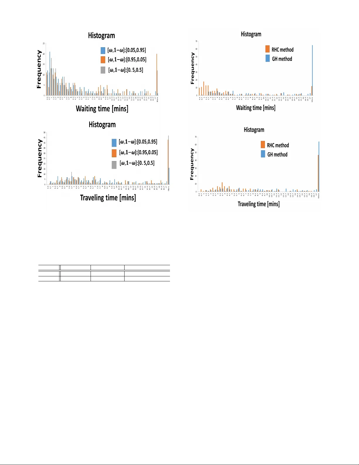
Optimization of Ride Sharing Systems Using Event-dri ven Receding Horizon Contr ol ? Rui Chen and Christos G. Cassandras Abstract — W e develop an e vent-driven Receding Horizon Control (RHC) scheme for a Ride Sharing System (RSS) in a transportation network where v ehicles are shar ed to pick up and drop off passengers so as to minimize a weighted sum of passenger waiting and trav eling times. The RSS is modeled as a discr ete ev ent system and the event-driven nature of the controller significantly r educes the complexity of the vehicle as- signment problem, thus enabling its real-time implementation. Simulation r esults using actual city maps and real taxi traffic data illustrate the effectiveness of the RH controller in terms of real-time implementation and performance relative to known greedy heuristics. I . I N T RO D U C T I O N It has been abundantly documented that the state of transportation systems worldwide is at a critical level. Based on the 2011 Urban Mobility Report, the cost of commuter delays has risen by 260% over the past 25 years and 28% of U.S. primary ener gy is no w used in transportation [1]. T raffic congestion also leads to an increase in v ehicle emissions; in large cities, as much as 90% of CO emissions are due to mobile sources. Disrupti ve technologies that aim at dramatically altering the transportation landscape include v ehicle connecti vity and automation as well as shared personalized transportation through emerging mobility-on- demand systems. Focusing on the latter , the main idea of a Ride Sharing System (RSS) is to assign vehicles in a giv en fleet so as to serve multiple passengers, thus effecti vely reducing the total number of vehicles on a road network, hence also congestion, energy consumption, and adverse en vironmental ef fects. The main objectives of a RSS are to minimize the total V ehicle-Miles-T raveled (VMT) over a giv en time period (equiv alently , minimize total trav el costs), to minimize the av erage waiting and trav eling times experienced by passen- gers, and to maximize the number of satisfied RSS partic- ipants (both drivers and passengers) [2]. When efficiently managed, a RSS has the potential to reduce the total number of priv ate vehicles in a transportation network, hence also decreasing ov erall energy consumption and traffic conges- tion, especially during peak hours of a day . From a passenger standpoint, a RSS is able to offer door-to-door transportation with minimal delays which makes trav eling more conv enient. From an operator’ s standpoint a RSS provides a considerable ? Supported in part by NSF under grants ECCS-1509084, CNS-1645681, and IIP-1430145, by AFOSR under grant F A9550-15-1-0471, by the DOE under grant DE-AR0000796, by the MathW orks and by Bosch. The authors are with the Division of Systems Engineering and Center for Information and Systems Engineering, Boston University , Brookline, MA 02446, USA { ruic,cgc } @bu.edu rev enue stream. A RSS also provides an alternati ve to public transportation or can work in conjunction with it to reduce possible lo w uitization of vehicles and long passenger delays. In this paper , we concentrate on designing dynamic v ehicle assignment strategies in a RSS aiming to minimize the system-wide waiting and traveling times of passengers. The main challenge in obtaining optimal vehicle assignments is the complexity of the optimization problem inv olved in conjunction with uncertainties such as random passenger service request times, origins, and destinations, as well as unpredictable traf fic conditions which determine the times to pick up and drop off passengers. Algorithms used in RSS are limited by the NP-complete nature of the underlying trav eling salesman problem [3] which is a special case of the much more complex problems encountered in RSS optimization. Therefore, a global optimal solution for such problems is generally intractable, ev en in the absence of the aforementioned uncertainties. Moreover , a critical require- ment in such algorithms is a guarantee that they can be implemented in a real-time conte xt. Sev eral methods have been proposed to solve the RSS problem addressing the waiting and traveling times of pas- sengers. In [4], a greedy approach is used to match vehicles to passenger requests which can on one hand guarantee real- time assignments but, on the other, lacks performance guar- antees. The optimization algorithm in [5] improves the aver - age traveling time performance but limits the seat capacity of each v ehicle to 2 (otherwise, the problem becomes intractable for 4 or more seats) and allows no dynamic allocation of new passengers after a solution is determined. Although vehicles can be dynamically allocated to passengers in [6], all pickup and drop-off ev ents are constrained to take place within a specified time window . The R TV -graph algorithm [7] can also dynamically allocate passengers, b ut its com- plexity increases dramatically with the number of agents (passengers and vehicles) and the seat capacity of vehicles. T o address the issue of increasing complexity with the size of a RSS, a hierarchical approach is proposed in [3] such that the system is decomposed into smaller regions. W ithin a re gion, a mixed-integer linear programs is formulated so as to obtain an optimal vehicle assignment ov er a sequence of fixed time horizons. Although this method addresses the complexity issue, it inv olves a large number of unnecessary calculations since there is no need to al ways re-ev aluate an optimal solution over every such horizon. Another approach to reducing complexity , is to abstract a RSS model through passenger and vehicle flo ws as in [8],[9] and [10]. In [10], for example, the interaction between autonomous mobility- on-demand and public transportation systems is considered so as to maximize the overall social welfare. In order to deal with the well-known “curse of dimension- ality” [11] that characterizes optimization problem formula- tions for a RSS, we adopt an event-driven Receding Horizon Contr ol (RHC) approach. This is in the same spirit as Model Predictiv e Control (MPC) techniques [12] with the added feature of exploiting the e vent-dri ven nature of the control process in which the RHC algorithm is in voked only when certain ev ents occur . Therefore, compared with con ventional time-driv en MPC this approach can a void unnecessary cal- culations and can significantly improv e the efficienc y of the RH controller by reacting to random ev ents as they occur in real time. The basic idea of event-dri ven RHC introduced in [13] and extended in [14] is to solve an optimization problem ov er a given planning horizon when an ev ent is observed in a way which allows vehicles to cooperate; the resulting control is then executed over a generally shorter action horizon defined by the occurrence of the next ev ent of interest to the controller . Compared to methods such as [5]-[7], the RHC scheme is not constrained by vehicle seating capacities and is specifically designed to dynamically re-allocate passengers to vehicles at any time. Moreover , compared to the time- driv en strategy in [3], the event-dri ven RHC scheme refrains from unnecessary calculations when no ev ent in the RSS occurs. Finally , in contrast to models used in [9] and [10], we maintain control of ev ery vehicle and passenger in a RSS at a microscopic level while ensuring that real-time optimal (over each receding horizon) vehicle assignments can be made. The paper is org anized as follows. W e first present in Section II a discrete ev ent system model of a RSS and formulate an optimization problem aimed at minimizing a weighted sum of passenger waiting and traveling times. Section III first re views the basic RHC scheme previously used and then identifies how it is limited in the conte xt of a RSS. This motiv ates the ne w RHC approach described in Section IV , specifically designed for a RSS. Extensi ve simulation results are giv en in Section V for actual maps in Ann Arbor, MI and New Y ork City , where, in the latter case, real taxi traf fic data are used to dri ve the simulation model. W e conclude the paper in Section VI. I I . P R O B L E M F O R M U L A T I O N W e consider a Ride Sharing System (RSS) in a traffic network consisting of N nodes N = { 1 , ..., N } where each node corresponds to an intersection. Nodes are connected by arcs (i.e., road segments). Thus, we view the traffic network as a directed graph G which is embedded in a two-dimensional Euclidean space and includes all points contained in every arc, i.e., G ⊂ R 2 . In this model, a node n ∈ N is associated with a point ν n ∈ G , the actual location of this intersection in the underlying two-dimensional space. The set of vehicles present in the RSS at time t is A ( t ) , where the index j ∈ A ( t ) will be used to uniquely denote a vehicle, and let A ( t ) = | A ( t ) | . The set of passengers is Fig. 1: A typical sample path of passenger i ’ s clock state z i ( t ) . P ( t ) , where the inde x i will be used to uniquely denote a passenger , and let P ( t ) = | P ( t ) | . Note that A ( t ) is time- varying since vehicles may enter or leave the RSS at any time and the same is true for P ( t ) . There are two points in G associated with each passenger i , denoted by o i , r i ∈ G : o i is the origin where the passenger issues a service request (pickup point) and r i is the passen- ger’ s destination (drop-of f point). Let O ( t ) = { o 1 , ..., o P } be the set of all passenger origins and R ( t ) = { r 1 , ..., r P } the corresponding destination set. V ehicles pick up passengers and deli ver them to their destinations according to some policy . W e assume that the times when vehicles join the RSS are not known in advance, but they become known as a vehicle joins the system. Similarly , the times when passenger service requests occur are random and their destinations become known only upon being picked up. State Space: In addition to A ( t ) and P ( t ) describing the state of the RSS, we define the states associated with each vehicle and passenger as follo ws. Let x j ( t ) ∈ G be the position of vehicle j at time t and let N j ( t ) ∈ { 0 , 1 , ..., C j } be the number of passengers in vehicle j at time t , where C j is the capacity of vehicle j . The state of passenger i is denoted by s i ( t ) where s i ( t ) = 0 if passenger i is waiting to be picked up and s i ( t ) = j ∈ A ( t ) , where j > 0, when the passenger is in vehicle j after being picked up. Finally , we associate with passenger i a left-continuous clock value z i ( t ) ∈ R whose dynamics are defined as follows: when the passenger joins the system and is added to P ( t ) , the initial value of z i ( t ) is 0 and we set ˙ z i ( t ) = 1, as illustrated in Fig.1 where the passenger service request time is ϕ i . Thus, z i ( t ) may be used to measure the waiting time of passenger i . When i is picked up by some vehicle j at time ρ i , j (see Fig.1), z i ( t ) is reset to zero and thereafter measures the trav eling time until the passenger’ s destination is reached at time σ i , j . In summary , the state of the RSS is X ( t ) = { A ( t ) , x 1 ( t ) , . . . , x A ( t ) , N 1 ( t ) , . . . , N A ( t ) , P ( t ) , s 1 ( t ) , . . . , s P ( t ) , z 1 ( t ) , . . . , z P ( t ) } . Events: All state transitions in the RSS are event-dri ven with the exception of the passenger clock states z i ( t ) , i ∈ P ( t ) , in which case it is the reset conditions (see Fig.1) that are event-dri ven. As we will see, all control actions (to be defined) affecting the state X ( t ) are taken only when an ev ent takes place. Therefore, regarding a v ehicle location x j ( t ) , j ∈ A ( t ) , for control purposes we are interested in its value only when events occur , e ven though we assume that x j ( t ) is av ailable to the RSS for all t based on an underlying localization system. W e define next the set E of all ev ents whose occurrence causes a state transition. W e set E = E U ∪ E C to dif ferentiate between uncontrollable events contained in E U and control- lable ev ents contained in E C . There are six possible ev ent types, defined as follows: (1) α i ∈ E U : a service request is issued by passenger i . (2) β j ∈ E U : vehicle j joins the RSS. (3) γ j ∈ E U : vehicle j leav es the RSS. (4) π i , j ∈ E C : vehicle j picks up passenger i (at o i ∈ G ). (5) δ i , j ∈ E C : vehicle j drops off passenger i (at r i ∈ G ). (6) ζ m , j ∈ E C : vehicle j arri ves at intersection (node) m ∈ N . Note that events α i , β j are uncontrollable exogenous ev ents. Event γ j is also uncontrollable, ho wev er it may not occur unless the “guard condition” N j ( t ) = 0 is satisfied, that is, the number of passengers in vehicle j must be zero when it leaves the system. On the other hand, the remaining three ev ents are controllable. First, π i , j depends on the control policy (to be defined) through which a v ehicle is assigned to a passenger and is feasible only when s i ( t ) = 0 and N j ( t ) < C j . Second, δ i , j is feasible only when s i ( t ) = j ∈ A ( t ) . Finally , ζ m , j depends on the policy (to be defined) and occurs when the route tak en by v ehicle j in volv es intersection m ∈ N . State Dynamics: The ev ents defined above determine the state dynamics as follows. (1) Event α i adds an element to the passenger set P ( t ) and increases its cardinality , i.e., P ( t + ) = P ( t ) + 1 where t is the occurrence time of this ev ent. In addition, it initializes the passenger state and associated clock: s i ( t + ) = 0 , ˙ z i ( t + ) = 1 with z i ( t ) = 0 (1) and generates the origin information of this passenger o i ∈ G . (2) Event β j adds an element to the vehicle set A ( t ) and increases its cardinality , i.e., A ( t + ) = A ( t ) + 1. It also initializes x j ( t ) to the location of vehicle j at time t . (3) Ev ent γ j remov es v ehicle j from A ( t ) and decreases its cardinality , i.e., A ( t + ) = A ( t ) − 1. (4) Event π i , j occurs when x j ( t ) = o i and it generates the destination information of this passenger r i ∈ G . This ev ent affects the states of both vehicle j and passenger i : N j ( t + ) = N j ( t ) + 1 , s i ( t + ) = j and, since the passenger w as just picked up, the associated clock is reset to 0 and starts measuring trav eling time tow ards the destination r i : z i ( t + ) = 0 , ˙ z i ( t + ) = 1 (2) (5) Event δ i , j occurs when x j ( t ) = r i and it causes a re- mov al of passenger i from P ( t ) and decreases its cardinality , i.e., P ( t + ) = P ( t ) − 1. In addition, it affects the state of vehicle j : N j ( t + ) = N j ( t ) − 1 (6) Event ζ m , j occurs when x j ( t ) = ν m . This event triggers a potential change in the control associated with v ehicle j as described ne xt. Control: The control we e xert is denoted by u j ( t ) ∈ G and sets the destination of vehicle j in the RSS. W e note that the destination u j ( t ) may change while vehicle j is en route to it based on new information receiv ed as various ev ents may take place. The control is initialized when ev ent β j occurs at some point x j ( t ) by setting u j ( t ) = ν m where m ∈ N is the intersection closest to x j ( t ) in the direction vehicle j is headed. Subsequently , the vector u ( t ) = { u 1 ( t ) , . . . , u A ( t ) } is updated according to a gi ven policy whenever an e vent from the set E occurs (we assume that all ev ents are observable by the RSS controller). Our control policy is designed to optimize the objecti ve function described ne xt. Objective Function: Our objective is to minimize the combined waiting and traveling times of passengers in the RSS over a given finite time interval [ 0 , T ] . In order to incorporate all passengers who hav e recei ved service ov er [ 0 , T ] , we define the set P T = ∪ t ∈ [ 0 , T ] P ( t ) to include all passengers i ∈ P ( t ) for any t ∈ [ 0 , T ] . In simple terms, P T is used to record all passengers who are either currently active in the RSS at t = T or were active and departed at some time t < T when the associated δ i , j ev ent occurred for some j ∈ A ( t ) . W e define w i to be the waiting time of passenger i and note that, according to (1), w i = z i ( t ) where t is the time when ev ent π i , j occurs. Similarly , letting y i be the total trav eling time of passenger i , according to (2) we have y i = z i ( t ) where t is the time when ev ent δ i , j occurs. W e then formulate the following problem, gi ven an initial state X 0 of the RSS: min u ( t ) E " ∑ i ∈ P T [ µ w w i + µ y y i ] # (3) where µ w , µ y are weight coef ficients defined so that µ w = ω W max and µ y = 1 − ω Y max , ω ∈ [ 0 , 1 ] , and W max and Y max are upper bounds of the waiting and traveling time of passengers respectiv ely . The values of W max and Y max are selected based on user experience to capture the worst case tolerated for waiting and traveling times respectiv ely . This construction ensures that w i and y i are properly normalized so that (3) is well-defined. The expectation in (3) is taken over all random e vent times in the RSS defined in an appropriate underlying probability space. Clearly , modeling the random ev ent processes so as to analytically e valuate this expectation is a dif ficult task. This motiv ates viewing the RSS as unfolding over time and adopting a control policy based on observed actual ev ents and on estimated future e vents that af fect the RSS state. Assuming for the moment that the system is deterministic, let t k denote the occurrence time of the k th event ov er [ 0 , T ] . A control action u ( t k ) may be taken at t k and, for simplicity , is henceforth denoted by u k . Along the same lines, Fig. 2: Ev ent-Driven receding horizon control. we denote the state X ( t k ) by X k . Letting K T be the number of ev ents observed ov er [ 0 , T ] , the optimal v alue of the objectiv e function when the initial state is X 0 is giv en by J ( X 0 ) = min u 0 , ··· u K T " ∑ i ∈ P T [ µ w w i + µ y y i ] # W e conv ert this into a maximization problem by considering [ − µ w w i − µ y y i ] for each i ∈ P T . Moreov er, observing that both w i and y i are upper-bounded by T , we consider the non- negati ve rewards T − w i and T − w i and rewrite the problem abov e as J ( X 0 ) = max u 0 , ··· u K T " ∑ i ∈ P T [ µ w ( T − w i ) + µ y ( T − y i )] # (4) Then, determining an optimal policy amounts to solving the following Dynamic Programming (DP) equation [11]: J ( X k ) = max u k ∈ G [ C ( X k , u k ) + J k + 1 ( X k + 1 )] , k = 0 , 1 , . . . , K T where C ( X k , u k ) is the immediate rew ard at state X k when control u k is applied and J k + 1 ( X k + 1 ) is the future reward at the next state X k + 1 . Our ability to solve this equation is limited by the well-known “curse of dimensionality” [11] ev en if our assumption that the RSS is fully deterministic were to be v alid. This further moti vates adopting a Receding Horizon Contr ol (RHC) approach as in similar problems en- countered in [13] and [14]. This is in the same spirit as Model Predictiv e Control (MPC) techniques [12] with the added feature of exploiting the e vent-dri ven nature of the control process. In particular, in the ev ent-driven RHC approach, a control action taken when the k th ev ent is observed is selected to maximize an immediate re ward defined ov er a planning horizon H k , denoted by C ( X k , u k , H k ) , followed by an estimated future reward ˆ J k + 1 ( X ( t k + H k )) when the state is X ( t k + H k ) . The optimal control action u ∗ k is, therefore, u ∗ k = arg max u k ∈ G [ C ( X k , u k , H k ) + ˆ J k + 1 ( X ( t k + H k ))] (5) The control action u ∗ k is subsequently e xecuted only over a generally shorter action horizon h k ≤ H k so that t k + 1 = t k + h k (see Fig.2). The selection of H k and h k will be discussed in the next section. I I I . R E C E D I N G H O R I Z O N C O N T R O L ( R H C ) In this section, we first re view the basic RHC scheme as introduced in [13], and a modified version in [14] intended to ov ercome some of the original scheme’ s limitations. W e refer to the RHC in [13] as RHC1 and the RHC in [14] as RHC2 . The basic RHC scheme in [13] considers a set of coop- erating “agents” and a set of “targets” in a Euclidean space. The purpose of agents is to visit targets and collect a certain time-varying reward associated with each target. The key steps of the scheme are as follows: (1) Determine a planning horizon H k at the current time t k . (2) Solv e an optimization problem to minimize an objecti ve function defined o ver the time interv al [ t k , t k + H k ] . (3) Determine an action horizon h k and execute the optimal solution over [ t k , t k + h k ] . (4) Set t k + 1 = t k + h k and return to step (1). Letting A ( t ) be the agent set and P ( t ) the target set, we define d i , j ( t ) for any i ∈ P ( t ) , j ∈ A ( t ) to be the distance between target i and agent j at time t . In [13], the planning horizon H k is defined as the earliest time that any agent can visit any target in the system: H k = min i ∈ P ( t ) , j ∈ A ( t )  d i , j ( t k ) v  (6) where v is the fixed speed of agents. The action horizon h k is defined to be the earliest time in [ t k , t k + H k ] when an event in the system occurs (e.g., a new target appears). In some cases, h k is alternatively defined through h k = ε H k for some ε ∈ ( 0 , 1 ] so as to ensure that h k ≤ H k . In order to formulate the optimization problem to be solved at every control action point t k , the concept of neighborhood for a target is defined in [13] as follows. The k th nearest agent neighbor to target l is β k ( l , t ) = arg min i ∈ A ( t ) , i 6 = β 1 l ( t ) ,..., i 6 = β k − 1 l ( t ) d l , i ( t ) where k = 1 , 2 , . . . , and the b -neighborhood of the target is giv en by the set of the b closest neighbors to it: B b l ( t ) = { β 1 ( l , t ) , . . . , β b ( l , t ) } (7) Based on (7), for any given b ≥ 1 the relative distance between agent i and tar get l is defined as ¯ d l , i ( t ) =    d l . i ( t ) ∑ q ∈ B b l ( t ) d l , q ( t ) 1 if i ∈ B b l ( t ) otherwise (8) Then, the relative responsibility function of agent i for target l is defined as: p ( ¯ d l , i ( t )) =        1 1 − Γ − ¯ d l , i 1 − 2 Γ 0 if ¯ d l , i ≤ Γ if Γ ≤ ¯ d l , i ≤ 1 − Γ otherwise (9) where p ( ¯ d l , i ( t )) can be viewed as the probability that agent i is the one to visit tar get l . In particular , when the relativ e distance is small, then i is committed to visit l , whereas if the relativ e distance is large, then i takes no responsibility for l . All other cases define a “cooperativ e region” where agent i visits l with some probability dependent on the parameter Γ which is selected so that Γ ∈ [ 0 , 1 2 ) and reflects a desired le vel of cooperation among agents; this cooperation le vel increases as Γ decreases. The use of p ( ¯ d l , i ( t )) allows the RHC to a void early commitments of agents to target visits, since changes in the system state may provide a better opportunity for an agent to improv e the overall system performance. A typical example arises when agent i is committed to target l and a new target, say l 0 , appears which is in close proximity to i ; in such a case, it may be beneficial for i to visit l 0 and let l become the responsibility of another agent that may be relati vely close to l and uncommitted. This is possible if p ( ¯ d l , i ( t )) < 1. In what follo ws, we will generalize the definition of distance d i , j ( t ) between tar get i and agent j to the distance between any two points x , y ∈ R 2 expressed as d ( x , y ) . Using the relativ e responsibility function, the optimization problem solved by the RHC at each control action point assigns an agent to a point which minimizes a gi ven objecti ve function and which is not necessarily a tar get point. Details of how this problem is set up and solved and the properties of the RHC1 scheme may be found in [13]. Limitations of RHC1 : There are three main limitations of the original RHC scheme: (1) Agent trajectory instabilities: A ke y benefit of RHC1 is the f act that early commitments of agents to targets are av oided. As already described above, if a new target appears in the system, an agent en route to a different tar get may change its trajectory to visit the new one if this is deemed beneficial to the cooperative system as a whole. This benefit, howe ver , is also a cause of potential instabilities when agents frequently modify their trajectories, thus potentially wasting time. It is also possible that an agent may oscillate between two targets and nev er visit either one. In [13], necessary and sufficient conditions were provided for some simple cases to quantify such instabilities, but these conditions may not always be satisfied. (2) Future cost estimation inaccuracies: The effecti veness of RHC1 rests on the accurac y of the future cost estimation term ˆ J k + 1 ( X ( t k + H k ) in (5). In [13], this future cost is estimated through its lower bound, thus resulting in an ov erly “optimistic” outlook. (3) Algorithm complexity: In [13], the optimization prob- lem at each algorithm iteration in volves the selection of each agent’ s heading over [ 0 , 2 π ] . This is because the plan- ning horizon H k defines a set of feasible reachable points F j ( t k , H k ) = { w : d ( w , x j ( t k ) = vH k } which is a disk of radius H k / v (where v is each agent’ s speed) around the agent’ s position at time t k . This problem must be solved over all agents and incurs considerable computational comple xity: if [ 0 , 2 π ] is discretized with discretization le vel G , then the complexity of this algorithm at each iteration is O ( G A ( t ) ) . The modified RCH scheme RHC2 in [14] was de veloped to address these limitations. T o deal with issues (1) and (3) above, a set of active targ ets S j ( t k , H k ) is defined for agent j at each iteration time t k . Its purpose is to limit the feasible reachable set F j ( t k , H k ) defined by all agent headings ov er [ 0 , 2 π ] so that it is reduced to a finite set of points. Let x ∈ F j ( t k , H k ) be a reachable point and define a travel cost function η i ( x , t ) associated with every target i ∈ P ( t ) measuring the cost of trav eling from a point x at time t to a target i ∈ P ( t ) . The active target set is defined in [14] as S j ( t k , H k ) = { l : l = arg min i ∈ P ( t ) η i ( x , t k + H k ) for some x ∈ F j ( t k , H k ) } (10) Clearly , S j ( t k , H k ) ⊆ P ( t ) is a finite set of targets defined by the following property: an activ e target is closer to some reachable point x than any other tar get in the sense of min- imizing the metric η i ( x , t k + H k ) . Therefore, if there is some target l 0 / ∈ S j ( t k , H k ) , then there is no incentiv e in considering it as a candidate for agent j to head towards. Restricting the feasible headings of an agent to its activ e target set not only reduces the complexity of optimally selecting a heading at t k , but it also limits oscillatory trajectory behavior , since by (6) there is always an active target on the set F j ( t k , H k ) so that ev entually all tar gets are guaranteed to be visited. Let u k be the control applied at time t k under planning horizon H k . The j th component of u k is the control u j ( t k ) applied to agent j , where u j ( t k ) ∈ S j ( t k , H k ) as defined in (10). The estimated time for agent j to reach a target u j ( t k ) is denoted by ˆ τ u , j ( u k , t k , H k ) where (for notational simplicity) we set u j ( t k ) = u . This time is gi ven by ˆ τ u , j ( u k , t k , H k ) = t k + H k + 1 v d ( x j ( t k ) , x u ) , u ∈ S j ( t k , H k ) (11) where x u is the location of tar get u = u j ( t k ) . T o address issue (2) regarding future cost estimation inaccuracies, a new estimation framew ork is introduced in [14] by defining a set of targets T k , j ⊆ P ( t ) − { u } that agent j would visit in the future, i.e., at t > t k + H k , as follo ws: T k , j = { l : p ( ¯ d l , j ( t k )) > p ( ¯ d l , q ( t k )) , ∀ q ∈ A ( t ) } (12) This set limits the targets considered by agent j to those with a current relativ e responsibility value in (9) which exceeds that of any other agent. The estimated time to reach a target l ∈ T k , j under control u k and planning horizon H k is denoted by ˆ τ l , j ( u k , t k , H k ) . The first tar- get to be visited in T k , j , denoted by l 1 , is the one with the minimal travel cost from target u ∈ S j ( t k , H k ) , i.e., l 1 = arg min l ∈ T k , j { η l ( x u , ˆ τ u , j ( u k , t k , H k )) } . Then, all sub- sequent targets in T k , j − { l 1 } are similarly ordered as { l 2 , l 3 , . . . } . Therefore, setting T n k , j = T k , j − { l 1 , . . . , l n − 1 } , n = 2 , . . . , | T k , j | , we ha ve l n + 1 = arg min l ∈ T n k , j { η l ( x l n , ˆ τ l n , j ( u k , t k , H k )) } , n = 1 , . . . , | T k , j | and ˆ τ l n + 1 , j ( u k , t k , H k ) = ˆ τ l n , j ( u k , t k , H k ) + 1 v d ( x l n , x l n + 1 ) (13) Limitations of the RHC2 with respect to a RSS : (1) Euclidean vs. Graph topology: Both RHC1 and RHC2 are based on an underlying Euclidean space topology . In a RSS, ho we ver , we are interested in a graph-based topology which requires the adoption of a dif ferent distance metric. (2) Future cost estimation inaccuracies : The travel cost metric η i ( x , t ) used in RHC2 assumes that all future targets to be visited at t > t k + H k are independent of each other and that an agent can visit any target. Howe ver , in a RSS, each agent j has a capacity limit C j . This has two implications: ( i ) If a vehicle is full, it must first be assigned to a drop-off point before it can visit a new pickup point, and ( ii ) The number of future pickup points is limited by C j − N j ( t ) , the residual capacity of vehicle j . The fact that there are two types of “targets” in a RSS (pickup points and drop-of f points), also induces an in- terdependence in the re wards associated with target visits. Whereas in [14] a reward is associated with each target visit, in a RSS the re wards are w i and y i where y i can only be collected after w i . This necessitates a new definition of the set T k , j in (12). For example, if i ∈ T k , j and vehicle j is full and must drop off a passenger at a remote location, then using (12) would cause vehicle j to first go to the drop-of f location and then return to pick up i ; howe ver , there may be a free vehicle k in the vicinity of j ’ s current location which is obviously a better choice to assign to passenger i . (3) Agent trajectory instabilities : RHC2 does not resolve the possibility of agent trajectory instabilities. Moreover , the nature of such instabilities is different due to the graph topology used in a RSS. In view of this discussion, we will present in the next section a new RHC scheme specifically designed for a RSS and addressing the issues identified above. W e will keep using the term “target” to refer to points o i and r i for all i ∈ P ( t ) . I V . T H E N E W R H C S C H E M E W e be gin by introducing some variables used in the new RHC scheme as follows. (1) d ( u , v ) is defined as the Manhattan distance [15] between two points u , v ∈ G . This measures the shortest path distance between two points on a directed graph that includes points on an arc of this graph which belong to G ⊂ R 2 . (2) R i , j ( t ) is the set of the n closest pickup locations in the sense of the Manhattan distance defined abov e, where n = C j − N j ( t ) − 1 if j picks up i at o i at time t , and n = C j − N j ( t ) + 1 if j drops off i at r i at time t . Clearly , the set may contain fewer than n elements if there are insuf ficient pickup locations in the RSS at time t . (3) ˆ R i , j ( t ) is the set of n drop-of f locations for j , where n = N j ( t ) + 1 if j picks up i at o i , and n = N j ( t ) − 1 if j drops off i at r i . (4) ϕ i and ρ i , j denote the occurrence time of events α i (passenger i joins the RSS) and π i , j (pickup of passenger i by vehicle j ) respectively . In the rest of this section we present the ne w RHC scheme which overcomes the issues previously discussed through four modifications: ( i ) W e define the travel value of a passenger for each vehicle considering the distance between vehicles and passengers, as well as the vehicle’ s residual capacity . ( ii ) Based on the new travel value and the graph topology of the map, we introduce a new active tar get set for each vehicle during [ t k , t k + H k ) . This allows us to reduce the feasible solution set of the optimization problem (5) at each iteration. ( iii ) W e de velop an improved future re ward estimation mechanism to better predict the time that a passenger is served in the future. ( iv ) T o address the potential instability problem, a method to restrain oscillations is introduced in the optimization algorithm at each iteration. Each of these modifications is described below , leading to the new RHC scheme. W e begin by defining the planning horizon H k at the k th control update consistent with (6) as H k = min i ∈ P ( t k ) , j ∈ A ( t k )  d ( x j ( t k ) , c i ) v j ( t k )  (14) where c i =  o i r i if s i ( t ) = 0 and N j ( t k ) < C j if s i ( t ) = j (15) and v j ( t k ) is the maximal speed of vehicle j at time t k , assumed to be maintained ov er [ t k , t k + H k ] . Thus, H k is the shortest Manhattan distance from any vehicle location to any target (either o i or r i ) at time t k . Note that c i is undefined if s i ( t ) = 0 and N j ( t k ) = C j . Formally , to ensure consistency , we set d ( x j ( t k ) , c i ) = ∞ if s i ( t ) = 0 and N j ( t k ) = C j since o i is not a valid pickup point for j in this case. The action horizon h k ≤ H k is defined by the occurrence of the next event in E , i.e., h k = τ k + 1 − t k where τ k + 1 is the time of the next event to occur after t k . If no such ev ent occurs over [ t k , t k + H k ] , we set h k = H k . A. V ehicle T ravel V alue Function Recall that in RHC2 a trav el cost function η i ( x , t ) was defined for any agent measuring the cost of traveling from a point x at time t to a target i ∈ P ( t ) . In our case, we define instead a travel value measuring the reward (rather than cost) associated with a vehicle j when it considers any passenger i ∈ P ( t ) . There are three cases to consider depending on the state s i ( t ) for any i ∈ P ( t ) as follows: Case 1: If s i ( t ) = 0, then passenger i is waiting to be picked up. From a vehicle j ’ s point of view , there are two components to the value of picking up this passenger at point o i : ( i ) The accumulated waiting time t − ϕ i of passenger i ; the larger this w aiting time, the higher the v alue of this passenger is. ( ii ) The distance of j from o i ; the shorter the distance, the higher the value of this passenger is. T o ensure this value component is non-negati ve, we define D to be the largest possible trav el time between any two points in the RSS (often referred to as the diameter of the underlying graph) and consider D − d ( x j ( t ) , o i ) as this value component. In order to properly normalize each component and ensure its associated value is restricted to the interval [ 0 , 1 ] , we use the waiting time upper bound W max introduced in (3) and the distance upper bound D to define the total travel v alue function as V i , j ( x j ( t ) , t ) = ( 1 − µ ) · t − ϕ i W max + µ · D − d ( x j ( t ) , o i ) D (16) where µ ∈ [ 0 , 1 ] is a weight coefficient depending on the relativ e importance the RSS places on passenger satisfaction (measured by waiting time) and vehicle distance traveled. In the latter case, a large v alue of d ( x j ( t ) , o i ) implies that vehicle j wastes time either trav eling empty (if N j ( t ) = 0) or adding to the traveling time of passengers already on board (if N j ( t ) > 0). Case 2: If s i ( t ) = j ∈ A ( t ) , then passenger i is already on board with destination r i . From vehicle j ’ s point of view , there are again two components to the v alue of deliv ering this passenger to point r i : ( i ) The accumulated tra vel time t − ρ i , j of passenger i . ( ii ) The distance of j from r i . Similar to (16), we define V i , j ( x j ( t ) , t ) = ( 1 − µ ) · t − ρ i , j Y max + µ · D − d ( x j ( t ) , r i ) D (17) where Y max is the travel time upper bound introduced in (3). Case 3: If s i ( t ) = k 6 = j , k ∈ A ( t ) , then passenger i is already on board some other vehicle k 6 = j . Therefore, from vehicle j ’ s point of vie w , the value of this passenger is V i , j ( x j ( t ) , t ) = 0. W e summarize the definition of the tra vel value function as follows: V i , j ( x j ( t ) , t ) =      ( 1 − µ ) · t − ϕ i W max + µ · D − d ( x j ( t ) , o i ) D if s i ( t ) = 0 ( 1 − µ ) · t − ρ i , j Y max + µ · D − d ( x j ( t ) , r i ) D if s i ( t ) = j 0 otherwise (18) In addition to this “immediate” v alue associated with pas- senger i , there is a future v alue for vehicle j to consider depending on the sets R i , j ( t ) and ˆ R i , j ( t ) defined earlier . In particular , if s i ( t ) = 0 and vehicle j proceeds to the pickup location o i , then the value associated with R i , j ( t ) is defined as V R i , j ( x j ( t ) , t ) = max n ∈ R i , j ( t ) V n , j ( o i , t ) which is the maximal tra vel value among all passengers in R i , j ( t ) to be collected if vehicle j selects o i as its destination at time t . On the other hand, if s i ( t ) = j and vehicle j proceeds to the drop-off location r i , then V n , j ( o i , t ) above is replaced by V n , j ( r i , t ) . Since the value of s i ( t ) is known to j , we will use c i as defined in (15) and write V R i , j ( x j ( t ) , t ) = max n ∈ R i , j ( t ) V n , j ( c i , t ) Similarly , the v alue of ˆ R i , j ( t ) is defined as V ˆ R i , j ( x j ( t ) , t ) = max n ∈ ˆ R i , j ( t ) V n , j ( c i , t ) W e then define the total travel v alue associated with a vehicle j when it considers an y passenger i ∈ P ( t ) as ¯ V i , j ( x j ( t ) , t ) = V i , j ( x j ( t ) , t ) + max { V R i , j ( x j ( t ) , t ) , V ˆ R i , j ( x j ( t ) , t ) } (19) Figure 3 shows an example of how ¯ V i , j ( x j ( t ) , t ) is ev aluated by vehicle j in the case where c i = o i (i.e., s i ( t ) = 0). In this case, R i , j ( t ) = { k , l , p } and ˆ R i , j ( t ) = { m , n } . Fig. 3: Tra vel value of passenger i ev aluated by vehicle j when s i ( t ) = 0. Fig. 4: Example of the reachability set of vehicle j . B. Active T arg et Sets The concept of an activ e target set was introduced in [14]. Clearly , this cannot be used in a RSS since the topology is no longer Euclidean and the trav el cost function η i ( x , t ) has been replaced by the tra vel value function (19). W e begin by defining the reachability (or feasible) set F j ( t k , H k ) for vehicle j in the RSS topology specified by G ⊂ R 2 . This is now a finite set consisting of horizon points in G reachable through some path starting from x j ( t k ) and assuming a fixed speed v j ( t k ) as defined in (14). This is illustrated in Fig. 4 where F j ( t k , H k ) consists of 10 horizon points (one-way streets hav e been taken into account as directed arcs in the underlying graph). Observ e that H k in this example is defined by o 2 , the pickup location of passenger 2 (horizon point 5) in accordance with (14). Note that since the actual speed of the vehicle may be lower than v j ( t k ) , it is possible that no horizon point is reached at time t k + h k ev en if h k = H k . This simply implies that a new planning horizon H k + 1 is ev aluated at t k + H k (which might still be defined by o 2 ).W e can no w define the acti ve target set of vehicle j to consist of any target (pickup or drop-off locations of passengers) which has the largest tra vel value to j for at least one horizon point x ∈ F j ( t k , H k ) . Definition: The set of Active T ar gets of vehicle j is defined as S j ( t k , H k ) = { l : l = arg max i ∈ P ( t ) ¯ V i , j ( x , t k + H k ) for some x ∈ F j ( t k , H k ) } (20) Observe that S j ( t k , H k ) ⊆ P ( t k ) and may reduce the number of passengers to consider as potential destinations assigned to j when S j ( t k , H k ) ⊂ P ( t k ) since u j ( t k ) ∈ S j ( t k , H k ) In the example of Fig. 4, P ( t k ) contains 6 passengers where s 1 ( t k ) = s 2 ( t k ) = s 4 ( t k ) = 0 and s 3 ( t k ) = s 5 ( t k ) = s 6 ( t k ) = j . Thus, we can immediately see that P ( t k ) = 6 <   F j ( t k , H k )   = 10. Further , observe that the drop-off points r 5 and r 6 are such that r 5 , r 6 / ∈ S j ( t k , H k ) since both points are farther away from x j ( t k ) than r 3 and o 2 respectiv ely . Therefore, the optimal control selection to be considered at t k is reduced to u j ( t k ) ∈ S j ( t k , H k ) = { o 1 , o 2 , r 3 , o 4 } . In addition, if the capacity C j happens to be such that C j = 3, then the only feasible control w ould be u j ( t k ) = r 3 . C. Futur e Rewar d Estimation In order to solve the optimization problem (5) at each RHC iteration time t k , we need to estimate the time that a future target is visited when t > t k + H k so as to ev aluate the term ˆ J k + 1 ( X ( t k + H k )) . Let us start by specifying the immediate reward term C ( X k , u k , H k ) in (5). In vie w of (4), there are three cases: ( i ) As a result of u k , an event π i , j (where s i ( t ) = j ) occurs at time t k + 1 with an associated rew ard C ( X k , u k , H k ) = µ w ( T − w i ) where w i = t k + 1 − ϕ i , ( ii ) As a result of u k , an ev ent δ i , j occurs at time t k + 1 with an associated reward C ( X k , u k , H k ) = µ y ( T − y i ) where y i = t k + 1 − ρ i , j , and ( iii ) Any other e vent results in no immediate rew ard. In summary , adopting the notation C ( u k , t k + 1 ) for the immediate reward resulting from control u k , we ha ve C ( u k , t k + 1 ) =    µ w ( T − w i ) if ev ent π i , j occurs at t k + 1 µ y ( T − y i ) if event δ i , j occurs at t k + 1 0 otherwise (21) In order to estimate future rew ards at times t > t k + 1 , recall that T k , j ⊆ P ( t ) − { u j ( t k ) } is a set of targets that vehicle j would visit in the future, after reaching u j ( t k ) . This set w as defined in [14] through (12) and a new definition suitable for the RSS will be gi ven below . Then, for each target n ∈ T k , j the associated rew ard is C ( u k , ˆ τ n , j ) where ˆ τ n , j is the estimated time that vehicle j reaches target n . If n = o i for some passenger i , then, from (21), C ( u k , ˆ τ n , j ) = µ w ( T − ˆ w i ) where ˆ w i = ˆ τ n , j − ϕ i , whereas if n = r i for some passenger i , then C ( u k , ˆ τ n , j ) = µ y ( T − ˆ y i ) where ˆ y i = ˆ τ n , j − ρ i , j . Further , we include a discount factor λ n ( ˆ τ n , j ) to account for the fact that the accuracy of our estimate ˆ τ n , j is monotonically decreasing with time, hence λ n ( ˆ τ n , j ) ∈ ( 0 , 1 ] . Therefore, for each vehicle j the associated term for ˆ J k + 1 ( X ( t k + H k )) is ˆ J j ( X ( t k + H k )) = | T k , j | ∑ n = 1 λ n ( ˆ τ n , j ) C ( u k , j , ˆ τ n , j ) (22) and ˆ J ( X ( t k + H k )) = ∑ j ∈ A ( t k ) ˆ J j ( X ( t k + H k )) (23) W e no w need to derive estimates ˆ τ n , j for each n ∈ T k , j . These estimates clearly depend on the order imposed on the elements of T k , j , i.e., the expected order that vehicle j follows in reaching the targets (after it reaches u j ( t k ) ) contained in this set. As already explained under (2) at the end of the last section, this order depends on the passenger states and the residual capacity of the v ehicle. Suppose that the order is specified through θ j n defined as the n th target label in T k , j (e.g., θ j 1 = 4 indicates that tar get 4 is the first to be visited). Then, (22) is re written as ˆ J j ( X ( t k + H k )) = | T k , j | ∑ n = 1 λ θ j n ( ˆ τ θ j n , j ) C ( u k , j , ˆ τ θ j n , j ) (24) It now remains to ( i ) define the set T k , j , suitably modified from (12) to apply to a RSS, so as to address the inaccuracy limitation (2) described at the end of the last section, and ( ii ) Specify the ordering { θ j 1 , . . . , θ j | T k , j | } imposed on the elements of T k , j . W e proceed by defining target subsets of T k , j ordered in terms of the priority of vehicle j to visit these targets compared to other v ehicles. This is done using the relativ e responsibility function in (9) with the Manhattan distance used in ev aluating ¯ d l , i ( t ) . Thus, let T k , j = T 1 k , j ∪ · · · ∪ T M k , j where T m k , j has the m th highest priority among all subsets and M ≤ P ( t ) is the number of subsets. When m = 1, we hav e T 1 k , j = { l : p ( ¯ d l , j ( t k )) > p ( ¯ d l , q ( t k )) , ∀ q ∈ A ( t ) , ∀ l ∈ P ( t ) } which is the same as (12): this is the passenger “responsi- bility set” of vehicle j in the sense that this vehicle has a higher responsibility value in (9) for each passenger in T 1 k , j than that of any other vehicle. Note that if s l ( t k ) = j , then by default we have l ∈ T 1 k , j since the drop-off location r i is the exclusi ve responsibility of v ehicle j . F or passengers with s l ( t k ) = 0, they are included in T 1 k , j as long as there is no other vehicle q 6 = j with a higher relati ve responsibility for l than that of j . Next, let A l , m ( t ) be a subset of vehicles defined as A l , m ( t k ) = { j : l / ∈ T n k , j , n < m , j ∈ A ( t k ) } This subset contains all vehicles which do not have target l included in an y of their top m − 1 priority subsets. W e then define T m k , j when m > 1 as follows: T m k , j = { l : p ( ¯ d l , j ( t k )) > p ( ¯ d l , q ( t k )) , ∀ q ∈ A l , m ( t k ) , ∀ l / ∈ T n k , j , n < m } (25) This set contains all targets for which j has a higher relativ e responsibility than an y other vehicle and which have not been included in any higher priority set T n k , j , n < m . As an example, suppose passenger i is waiting to be picked up and belongs to T 1 k , j 1 , T 2 k , j 2 and T 3 k , j 3 , where j 1 is the closest vehicle to i . Suppose vehicle j 1 is full and needs to drop off a passenger first whose destination is far away . Because vehicle j 2 has the 2nd highest priority , then j 2 may serv e i provided it has av ailable seating capacity . If j 2 cannot serve i , then vehicle j 3 with a lower priority is the next to consider serving i . In this manner, we overcome the limitation of (12) where no agent capacity is taken into account. The last step is to specify the ordering { θ j 1 , . . . , θ j    T m k , j    } imposed on each set T m k , j , j ∈ A ( t ) , m = 1 , . . . , M . This is accomplished by using the travel v alue function ¯ V i , j ( x j ( t ) , t ) in (19) as follows: ¯ V θ j n + 1 , j ( c θ j n , ˆ τ θ j n , j ) ≤ ¯ V i , j ( c θ j n , ˆ τ θ j n , j ) (26) for all i ∈ T m k , j − { θ j 1 , . . . , θ j n } where we have used the definition of c i in (15). Setting u = u j ( t k ) , the estimated times are given by ˆ τ θ j 1 , j = t k + 1 v d ( x j ( t k ) , x u ) + 1 v d ( u , c θ j 1 , j ) (27) ˆ τ θ j n , j = ˆ τ θ j n − 1 , j + 1 v d ( c θ j n − 1 , j , c θ j n , j ) , n > 1 (28) where ˆ τ θ j 1 , j is the estimated time of reaching the target with the highest travel value beyond the one selected as u j ( t k ) among all targets in T m k , j and ˆ τ θ j n , j for n > 1 is the estimated time of reaching the n th target in the order established through (26). Note that this approach takes into account the state of v ehicle j ; in particular, if N j ( t ) = C j , then the ordering of targets in T m k , j is limited to those such that s i ( t k ) = j . This completes the ev aluation of the estimated future rew ard in (23) based on (21) and (22), along with the ordering of future targets specified through (26). D. Pr eventing V ehicle T rajectory Instabilities Our final concern is the issue of instabilities discussed under (3) at the end of the last section. This problem arises when a new passenger joins the system and introduces a new target for one or more v ehicles in its vicinity which may hav e higher travel value in the sense of (19) than current ones. As a result, a vehicle may switch its current destination u j ( t k ) and this process may repeat itself with additional future new passengers. In order to av oid frequent such switches, we introduce a threshold parameter denoted by Θ and react to any event α i (a service request issued by a new passenger i ) that occurs at time t k as follows: u j ( t k ) =    o i if ¯ V i , j ( x j ( t k ) , o i ) − ¯ V u , j ( x j ( t k ) , x u ) > Θ , N j ( t ) < C j , j = 1 , . . . , A ( t k ) u otherwise (29) where u = u j ( t k − 1 ) is the current destination of j . In simple terms, the current control remains unaf fected unless the new passenger provides an incremental value relativ e to this control which e xceeds a given threshold. Since (29) is applied to all vehicles in the current v ehicle set A ( t ) , the vehicle with the largest incremental travel v alue ends up with o i as its control as long as it exceeds Θ . Note that the ne w passenger may not be assigned to j unless this vehicle has a positiv e residual capacity . E. RHC optimization sc heme The RHC scheme consists of a sequence of optimization problems solved at each e vent time t k , k = 1 , 2 , . . . with each problem of the form u ∗ k = ar g max u k , j ∈ S j ( t k , H k ) j ∈ A ( t k ) [ C ( u k , t k + 1 ) + ∑ j ∈ A ( t k )    T m k , j    ∑ n = 1 λ θ j n ( ˆ τ θ j n , j ) C ( u k , j , ˆ τ θ j n , j )] , m = 1 , . . . , M (30) where S j ( t k , H k ) is the active target of vehicle j at time t k ob- tained through (20), C ( u k , t k + 1 ) is given by (21), and ˆ τ θ j n , j is ev aluated through (27)-(28) with the ordering { θ j 1 , . . . , θ j    T m k , j    } giv en by (26) and the sets T m k , j , m = 1 , . . . , M , defined through (25). Note that (30) must be augmented to include (29) when the ev ent occurring at t k is of type α i . An algorithmic description of the RHC scheme is gi ven in Algorithm 1 1) Determine H k through (14); 2) Determine the active target set S j ( t k , H k ) through (20) for all j ∈ A ( t ) ; 3) Evaluate the estimated future reward through (27) and (28) for all candidate optimal controls; 4) Determine the optimal control u ∗ k in (30); 5) Execute u ∗ k until an e vent occurs; if a ne w passenger i enter s the system then for each vehicle j with N j ( t ) < C j do calculate ¯ V i , j ( x j ( t k ) , o i ) ; if ¯ V i , j ( x j ( t k ) , o i ) − ¯ V u , j ( x j ( t k ) , x u ) > Θ then we set i as the new target; break; end end end Algorithm 1: RHC Algorithm. Complexity of Algorithm 1: The complexity of the original RHC in [13] was discussed in Section III. For the new RHC we have dev eloped, the optimal control for vehicle j at any iteration is selected from the finite set S j ( t k , H k ) defined by active targets. Thus, the complexity is O ( Ω A ( t ) ) where Ω ≤ P ( t ) (the number of targets) is the maximum number of activ e targets. Observe that Ω decreases as targets are visited if new ones are not generated. V . S I M U L A T I O N R E S U LT S W e use the SUMO (Simulation of Urban Mobility) [16] transportation system simulator to e valuate our RHC for a RSS applied to tw o traffic networks (in Ann Arbor, MI and in New Y ork City , NY). Among other con venient features, Fig. 5: A RSS in the Ann Arbor map. SUMO may be employed to simulate large-scale traffic networks and to use traffic data and maps from other sources, such as OpenStreetMap and VISUM. V ehicle speeds are set by the simulation and they include random factors like different road speed limits, turns, traf fic lights, etc. A. RHC for a RSS in the Ann Arbor map A RSS for part of the Ann Arbor map is shown in Fig.5. Green colored vehicles are idle while red colored ones contain passengers to be serv ed. A triangle along a road indicates a waiting passenger . W e pre-load in SUMO a fixed number of v ehicles, while passengers request service at random points in time as the simulation runs. Passenger arriv als are modeled as a Poisson process with a rate of 3 passengers/min. The remaining RSS system parameters are selected as follows: C j = 4, T = 300 min, W max = 47 min, Y max = 47 min, D = 3000 m and the threshold in (29) is set at Θ = 0 . 3. In T able I, the a verage waiting and trav eling times under RHC are shown for different weights ω in the Ann Arbor RSS. The results are av eraged ov er three independent simula- tion runs. In this example, the number of pre-loaded vehicles is 7 and simulations end after 30 passengers are delivered to associated destinations (which is within T=300 min set abov e). In order to e valuate the performance of the RSS at steady state, we allow a simulation to “warm up” before starting to measure the 30 passengers served over the course of a simulation run. The first column of T able I shows different values of the weights ω as defined in (3) specifying the relativ e importance assigned to passenger waiting and traveling respecti vely . As expected, emphasizing waiting results in larger vehicle occupancy and longer av erage trav el times. In Fig. 6 we provide the waiting and tra veling time histograms for all cases in T able I. In T able II, we compare our RHC method with a greedy heuristic (GH) algorithm (similar to [4]) which operates as follows. When passenger i joins the RSS and generates the Fig. 6: W aiting and traveling time histograms under different weights ω for the Ann Arbor RSS. pickup point o i , we ev aluate the incremental cost this point incurs to vehicle j ∈ A ( t ) when placed in every possible position in this vehicle’ s current destination sequence, as long as the capacity constraint N j ( t ) < C j is never violated. The optimal position is the one that minimizes this incre- mental cost. Once this is done for all vehicles j ∈ A ( t ) , we select the minimal incremental cost incurred among all vehicles. Then, passenger i is assigned to the associated vehicle. As seen in T able II with ω = 0 . 5, the RHC algorithm achiev es a substantially better weighted sum performance (approximately by a factor of 2) which are averaged ov er three independent simulation runs. In Fig. 7 we compare the associated waiting and trav eling time histograms showing in greater detail the substantially better performance of RHC relativ e to GH. T able III compares different vehicle numbers when the deliv ered passenger number is 30 showing waiting and tra veling times, vehicle occupanc y and the objectiv e in (3). The lar ger the vehicle number , the better the performance can be achie ved. B. RHC for a RSS in the New Y ork City map A RSS covering an area of 10 × 10 blocks in New Y ork City is shown in Fig.8. In this case, we generate passenger arri vals based on actual data from the NYC T axi Fig. 7: Comparison of waiting and trav eling time histograms under RHC and GH for the Ann Arbor RSS ( ω = 0 . 5). T ABLE I: A verage waiting and tra veling times under RHC for different weights ω in the Ann Arbor RSS [ ω , 1 − ω ] W aiting Time [mins] Tra veling Time [mins] V ehicle Occupancy [ 0 . 05 , 0 . 95 ] 6.5 4.1 1.62 [ 0 . 5 , 0 . 5 ] 6.0 5.2 2.64 [ 0 . 95 , 0 . 05 ] 6.2 5.6 3.02 Fig. 8: A RSS co vering an area of 10 × 10 blocks in Ne w Y ork City . T ABLE II: A verage waiting and traveling time [mins] com- parisons for different RSS control methods in the Ann Arbor RSS when ω = 0 . 5 Method W aiting Time Trav eling Time W eighted Sum in (3) RHC 6.5 4.1 0.113 GH 9.6 9.7 0.205 T ABLE III: A verage waiting and trav eling time [mins] com- parisons for different numbers of vehicles in the Ann Arbor RSS when ω = 0 . 5 under the RHC method V ehicle Numbers W aiting Time Tra veling Time V ehicle Occupancy W eighted Sum in (3) 4 11.0 5.5 2.93 0.176 7 6.5 4.1 2.64 0.113 and Limousine Commission which provides exact timing of arriv als and the associated origins and destinations. W e pre- loaded 8 vehicles and run the simulations until 50 passengers are served based on actual data from a weekday of January , 2016 (the approximate passenger rate is 16 passengers/min). All other RSS settings are the same as before. In T able IV, the average waiting and traveling times under RHC are sho wn for dif ferent weights ω in the Ne w Y ork City RSS. The results are av eraged over three independent simulation runs. The first column of T able IV shows dif- ferent values of the weights ω as defined in (3) specifying the relativ e importance assigned to passenger waiting and trav eling resepctively . As in the case of the Ann Arbor RSS, emphasizing waiting results in larger vehicle occupancy with longer average trav el times. In Fig. 9 we provide the waiting and traveling time histograms for all cases in T able IV. In T able V, we compare RHC with ω = 0 . 5 with the aforementioned greedy heuristic algorithm GH in terms of the average waiting and trav eling times. W e can see once again that the RHC algorithm achieves a substantially better performance. In Fig.10 we compare the associated waiting and traveling time histograms for RHC relativ e to GH. W e have also tested a relativ ely long RSS operation based T ABLE IV: A verage waiting and trav eling times under RHC for dif ferent weights ω in the Ne w Y ork City RSS with 8 vehicles. [ ω , 1 − ω ] W aiting Time [mins] Tra veling Time [mins] V ehicle Occupancy [ 0 . 05 , 0 . 95 ] 9.1 7.8 1.96 [ 0 . 5 , 0 . 5 ] 11.9 9.0 2.59 [ 0 . 95 , 0 . 05 ] 10.3 10.2 3.06 T ABLE V: A verage waiting and traveling time [mins] com- parisons for different RSS control methods in the New Y ork City RSS with 8 v ehicles and ω = 0 . 5. Method W aiting Time Trav eling Time W eighted Sum in (3) RHC 11.9 9.0 0.222 GH 21.5 17.0 0.410 Fig. 9: W aiting and traveling time histograms under different weights ω for the New Y ork City RSS with 8 v ehicles. T ABLE VI: A verage waiting and trav eling times under RHC for dif ferent weights ω in the New Y ork City RSS with 28 vehicles. [ ω , 1 − ω ] W aiting time [mins] T raveling time [mins] V ehicle Occupancy [ 0 . 05 , 0 . 95 ] 4.1 8.1 2.07 [ 0 . 5 , 0 . 5 ] 5.2 12.4 2.79 [ 0 . 95 , 0 . 05 ] 7.0 12.6 2.83 on actual passenger data from a weekday of January 2016 which is the same as before for the shorter time intervals. W e pre-loaded 28 vehicles and run simulations until 160 passengers are served. All other settings are the same as before. T able VI shows the associated waiting and traveling times under different weights with similar results as before. Figure 11 shows the associated waiting and trav eling time his- tograms for all cases in T able VI. In T able VII, we compare RHC to the GH algorithm in terms of the av erage waiting and trav eling times with results consistent with those of T able V. T able VIII compares different v ehicle numbers when the deliv ered passenger number is 160 showing waiting and trav eling times, v ehicle occupancy and the objectiv e in (3) whose performance is consistent with that of T able III. T able IX shows real execution times for our RHC regard- ing different vehicle and passenger numbers. Fig. 10: Comparison of waiting and tra veling time histograms under RHC and GH in the New Y ork City RSS with 8 vehicles. T ABLE VII: A verage waiting and trav eling time [mins] comparisons under RHC and GH in the New Y ork City RSS with 28 v ehicles and ω = 0 . 5. Method W aiting time Trav eling time W eighted Sum in (3) RHC 5.2 12.4 0.187 GH 16.1 16.6 0.348 T ABLE VIII: A verage waiting and traveling time [mins] comparisons for different numbers of vehicles in the New Y ork City RSS when ω = 0 . 5 and the deliv ered passenger number is 160 under the RHC method V ehicle Numbers W aiting Time Tra veling Time V ehicle Occupancy W eighted Sum in (3) 28 5.2 12.4 2.79 0.187 38 3.5 10.7 2.31 0.151 T ABLE IX: A verage real ex ecution time for our RHC ALGO. when ω = 0 . 5 V ehicle Numbers Passenger Numbers A verage Execution Time [sec] 8 50 3 28 160 17 38 160 19 Fig. 11: W aiting and traveling time histograms under differ - ent weights ω for the New Y ork City RSS with 28 vehicles. T ABLE X: A verage waiting and traveling time [mins] com- parisons under RHC and GH in the Ne w Y ork City RSS with 38 vehicles and ω = 0 . 5. Method W aiting time Trav eling time W eighted Sum in (3) RHC 19.1 13.7 0.349 GH 61.4 19.0 0.855 Finally , we tested a relatively longer RSS operation with 38 v ehicles based on the same actual passenger data as before which generates 1000 passengers ov er approximately 1 . 2 ’ real’ operation hours. Simulations will not end until 900 passengers are deli vered. In T able X, we compare RHC to the GH algorithm in terms of the average waiting and tra veling times with results consistent with those of T able V. V I . C O N C L U S I O N S A N D F U T U R E W O R K An e vent-dri ven RHC scheme is de veloped for a RSS where vehicles are shared to pick up ad drop off passengers so as to minimize a weighted sum of passenger waiting and trav eling times. The RSS is modeled as a discrete event system whose e vent-driv en nature significantly reduces the complexity of the vehicle assignment problem, thus enabling its implementation in a real-time context. Simulation results adopting actual city maps and real taxi traffic data show the effecti veness of the RHC controller in terms of real-time implementation and performance relati ve to known greedy Fig. 12: Comparisons of waiting and trav eling time his- tograms between the RHC and GH methods in the New Y ork City RSS when the v ehicle number is 28. heuristics. In our ongoing w ork, an important problem we are considering is where to optimally position idle vehicles so that they are best used upon receiving future calls. Moreov er , depending on real ex ecution times of our RHC algorithm (see T able IX), we will use this information as a rational measure for decomposing a map into regions such that within each region the RHC vehicle assignment response times remain manageable. R E F E R E N C E S [1] D. Schrank, T . Lomax, and B. E. TTIs, “Urban mobility report. texas transportation institute, the texas a and m university system, 2007, ” 2011. [2] N. Agatz, A. Erera, M. Savelsber gh, and X. W ang, “Optimization for dynamic ride-sharing: A review , ” Eur opean J ournal of Oper ational Resear ch , vol. 223, no. 2, pp. 295–303, 2012. [3] X. Chen, F . Miao, G. J. Pappas, and V . Preciado, “Hierarchical data- driv en vehicle dispatch and ride-sharing, ” in Decision and Contr ol (CDC), 2017 IEEE 56th Annual Confer ence on . IEEE, 2017, pp. 4458–4463. [4] N. A. Agatz, A. L. Erera, M. W . Savelsber gh, and X. W ang, “Dynamic ride-sharing: A simulation study in metro atlanta, ” T ransportation Resear ch P art B: Methodological , v ol. 45, no. 9, pp. 1450–1464, 2011. [5] P . Santi, G. Resta, M. Szell, S. Sobolevsky , S. H. Strogatz, and C. Ratti, “Quantifying the benefits of vehicle pooling with shareability networks, ” Pr oceedings of the National Academy of Sciences , vol. 111, no. 37, pp. 13 290–13 294, 2014. [6] G. Berbeglia, J.-F . Cordeau, and G. Laporte, “Dynamic pickup and deliv ery problems, ” Eur opean journal of operational resear ch , vol. 202, no. 1, pp. 8–15, 2010. [7] J. Alonso-Mora, S. Samaranayake, A. W allar, E. Frazzoli, and D. Rus, “On-demand high-capacity ride-sharing via dynamic trip-vehicle as- signment, ” Pr oceedings of the National Academy of Sciences , vol. 114, no. 3, pp. 462–467, 2017. [8] G. C. Calafiore, C. Nov ara, F . Portigliotti, and A. Rizzo, “ A flo w optimization approach for the rebalancing of mobility on demand systems, ” in Decision and Contr ol (CDC), 2017 IEEE 56th Annual Confer ence on . IEEE, 2017, pp. 5684–5689. [9] M. Tsao, R. Iglesias, and M. Pav one, “Stochastic model predic- tiv e control for autonomous mobility on demand, ” arXiv preprint arXiv:1804.11074 , 2018. [10] M. Salazar, F . Rossi, M. Schiffer , C. H. Onder , and M. Pav one, “On the interaction between autonomous mobility-on-demand and public transportation systems, ” arXiv preprint , 2018. [11] D. P . Bertsekas, D. P . Bertsekas, D. P . Bertsekas, and D. P . Bertsekas, Dynamic pr ogramming and optimal contr ol . Athena scientific Bel- mont, MA, 2005, vol. 1, no. 3. [12] E. F . Camacho and C. B. Alba, Model pr edictive contr ol . Springer Science & Business Media, 2013. [13] W . Li and C. G. Cassandras, “ A cooperati ve receding horizon con- troller for multivehicle uncertain environments, ” IEEE T ransactions on Automatic Control , vol. 51, no. 2, pp. 242–257, 2006. [14] Y . Khazaeni and C. G. Cassandras, “Event-driven cooperati ve receding horizon control for multi-agent systems in uncertain en vironments, ” IEEE T ransactions on Contr ol of Network Systems , 2016. [15] J. S. Farris, “Estimating phylogenetic trees from distance matrices, ” The American Naturalist , vol. 106, no. 951, pp. 645–668, 1972. [16] G. A. C. (DLR). (2017) Simulation of urban mobility . [Online]. A vailable: http://www .sumo.dlr .de/userdoc/Contact.html