Sparse Polynomial Zonotopes: A Novel Set Representation for Reachability Analysis

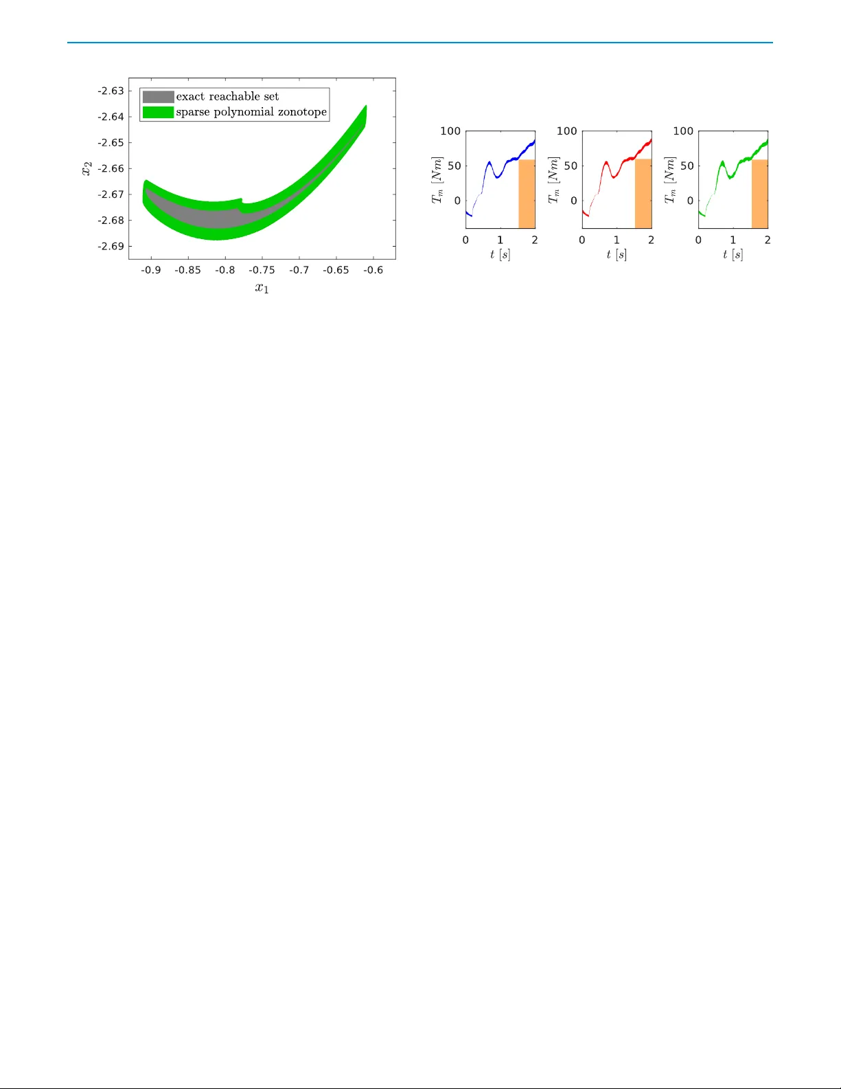
GENERIC COLORIZED JOURNAL, V OL. XX, NO . XX, XXXX 2017 1 Sparse P olynomial Zonotopes: A No v el Set Representation f or Reachability Analysis Niklas K ochdumper , Matthias Althoff Abstract — W e introduce spar se polynomial zonotopes , a ne w set representation for formal verification of h ybrid systems. Sparse polynomial zonotopes can represent non- con vex sets and are g eneralizations of zonotopes, poly- topes, and T aylor models. Operations like Minkowski sum, quadratic mapping, and reduction of the representation size can be computed with polynomial complexity w .r .t. the dimension of the system. In particular , for reachabil- ity analysis of nonlinear systems, the wrapping eff ect is substantially reduced using sparse pol ynomial zonotopes, as demonstrated by numerical examples. In addition, we can significantly reduce the computation time compared to zonotopes when dealing with nonlinear dynamics. Index T erms — Reachability analysis, nonlinear dynam- ics, hybrid systems, spar se polynomial zonotopes. I . I N T R O D U C T I O N E FFICIENT set representations are highly rele v ant for controller synthesis and formal verification of hybrid systems, since many underlying algorithms compute with sets; see e.g., [18], [38], [60], [63]. Improv ements originating from a ne w set representation often significantly reduce computation time and improve the accuracy of set-based computations. A. State of the Ar t Fig. 1 shows rele v ant set representations and their relations to each other . Almost all typical set representations are con vex, except T aylor models, star sets, lev el sets, and polynomial zonotopes. Since all con ve x sets can be represented by support functions, which are closed under Minko wski addition, linear maps, and con vex hull operations, they are a good choice for reachability analysis [28], [29], [32], [55], [59]. Ellipsoids and polytopes are special cases of support functions, which are often used for reachability analysis [17], [22], [24], [44], [59] and computations of inv ariant sets [3], [16], [45], [57]. Ho w- ev er , the disadvantage of ellipsoids is that they are not closed under intersection and Minkowski addition; the disadv antage of polytopes is that the Minko wski sum is computationally expensi v e [62]. One important subclass of polytopes is zonotopes, which can be represented compactly by so-called generators: a This paragr aph of the first footnote will contain the date on which you submitted your paper f or re view . This work was suppor ted b y the Ger man Research Foundation (DFG) project f av eA C under gr ant number AL 1185/5-1 Niklas K ochdumper and Matthias Althoff are both with the Depar tment of Computer Science , T echnical University of Munich, 85748 Garching, Germany (e-mail: niklas.kochdumper@tum.de , althoff@tum.de). Polyno mia l Zonotop es Supp ort F unc tion s Polytop es Const rai ned Zonotop es Zonotop e Bundl es Elli psoi ds Zonotop es T a ylor Model s Inter vals Star Sets Level Sets Conve x Non-conve x Fig. 1 : V isualization of the relations between the dif ferent set representations, where A → B denotes that B is a generalization of A. zonotope with l generators in n dimensions might have up to  l n − 1  halfspaces. More importantly , Mink owski sum and linear maps can be computed cheaply , making them a good choice for reachability analysis [8], [31], [34], [35], [59]. Zonotopes are closely related to affine arithmetic [25] with the zonotope factors being identical to the noise symbols in affine arithmetic. T wo relev ant extensions to zonotopes are zonotope bundles [10], where the set is represented implicitly by the intersection of several zonotopes, and constrained zonotopes [61], where additional equality constraints on the zonotope f ac- tors are considered. Zonotope bundles, as well as constrained zonotopes, are both able to represent any bounded polytope. Both representations make use of lazy computations and thus suffer much less from the curse of dimensionality , as is the case for polytopes [62]. T wo other set representations related to zonotopes are comple x zonotopes [1] and zonotopes with sub-polyhedric domains [30]. Complex zonotopes are defined by comple x valued vectors and are well-suited to verify global exponential stability for systems with complex v alued eigen- vectors [1]. Zonotopes with sub-polyhedric domains use zones, octagons, and polyhedra instead of intervals to represent the domain for the zonotope factors, which enables the efficient computation of intersections and unions of sets by exploiting lazy computations [30]. A special case of zonotopes are multi- dimensional interv als, which are particularly useful for range bounding of nonlinear functions via interval arithmetic [37], but they are also used for reachability analysis [27], [54]. Since intervals are not closed under linear maps, one often has to split them to reduce the wrapping effect [46]. In general, reachable sets of nonlinear systems are non- con v ex, so that tight enclosures can only be achieved using non-con v ex set representations when av oiding the splitting of reachable sets. T aylor models [49], which consist of a 2 GENERIC COLORIZED JOURNAL, V OL. XX, NO . XX, XXXX 2017 polynomial and an interval remainder part, are an example of non-con v ex set representation. They are typically used for range bounding [50] and reachability analysis [20], [21], [48], [53]. Polynomial zonotopes, another type of non-conv ex set representation, are introduced in [5] and can equally represent the set defined by a T aylor model, as later shown in this work. Quadratic zonotopes [2] are a special case of polynomial zonotopes. T wo other ways to represent non-con vex sets are star sets, which are especially useful for simulation-based reachability analysis [14], [26], and level sets of nonlinear functions [51], which are applied to compute reachable sets [52] and controlled in v ariant regions [43]. While star sets and lev el sets are very expressi v e, it is yet unclear how some operations, such as nonlinear mapping, are computed. B. Over view In this work, we introduce a new non-con ve x set rep- resentation called sparse polynomial zonotopes , which is a non-trivial extension of polynomial zonotopes from [5] and exhibits the follo wing major advantages: a) sparse polynomial zonotopes enable a very compact representation of sets, b) they are closed under all relev ant operations, c) many other set representations can be conv erted to a sparse polynomial zonotope, and most importantly , d) all operations ha ve at most polynomial complexity . The remainder of this paper is structured as follo ws: In Sec. II, the formal definition of sparse polynomial zonotopes is provided and important operations on them are deriv ed. W e show how sparse polynomial zonotopes provide substantially better results for reachability analysis in Sec. III, which is demonstrated in Sec. IV on four numerical examples. C . Notation In the remainder of this paper , we will use the following notations: Sets are always denoted by calligraphic letters, matrices by uppercase letters, and vectors by lowercase letters. Giv en a discrete set H ∈ {·} n , |H| = n denotes the cardinality of the set. Given a vector b ∈ R n , b ( i ) refers to the i -th entry . Giv en a matrix A ∈ R n × m , A ( i, · ) represents the i -th matrix ro w , A ( · ,j ) the j -th column, and A ( i,j ) the j -th entry of matrix row i . Given a discrete set of positive integer indices H = { h 1 , . . . , h |H| } with 1 ≤ h i ≤ m ∀ i ∈ { 1 , . . . , |H|} , A ( · , H ) is used for [ A ( · ,h 1 ) . . . A ( · ,h |H| ) ] , where [ C D ] denotes the concatenation of two matrices C and D . The symbols 0 ( n,m ) ∈ R n × m and 1 ( n,m ) ∈ R n × m represent matrices of zeros and ones, and I n ∈ R n × n is the identity matrix. The empty matrix is denoted by [ ] . The left multiplication of a matrix M ∈ R m × n with a set S ⊂ R n is defined as M ⊗ S = { M s | s ∈ S } , the Minkowski addition of two sets S 1 ⊂ R n and S 2 ⊂ R n is defined as S 1 ⊕ S 2 = { s 1 + s 2 | s 1 ∈ S 1 , s 2 ∈ S 2 } , and the Cartesian product of two sets S 1 ⊂ R n and S 2 ⊂ R m is defined as S 1 × S 2 = { [ s 1 s 2 ] T | s 1 ∈ S 1 , s 2 ∈ S 2 } . W e further introduce an n - dimensional interval as I = [ l , u ] , ∀ i l ( i ) ≤ u ( i ) , l , u ∈ R n . The Nabla operator is defined as ∇ = P n i =1 e i ∂ ∂ x ( i ) , with x ∈ R n and e i ∈ R n being orthogonal unit vectors. For the deriv ation of computational complexity , we consider all (a) (b) (c) (d) Fig. 2 : Construction of the SPZ in Example 1 from the single generator vectors. binary operations e xcept concatenations, and initializations are explicitly not considered. I I . S P A R S E P O L Y N O M I A L Z O N O T O P E S Let us first define sparse polynomial zonotopes (SPZs), followed by deriv ations of relev ant operations on them. Definition 1: (Sparse P olynomial Zonotope) Given a genera- tor matrix of dependent generator s G ∈ R n × h , a generator matrix of independent generator s G I ∈ R n × q , and an expo- nent matrix E ∈ N p × h 0 , an SPZ is defined as P Z =  h X i =1  p Y k =1 α E ( k,i ) k  G ( · ,i ) + q X j =1 β j G I ( · ,j )     α k , β j ∈ [ − 1 , 1]  . (1) The scalars α k are called dependent factors since a change in their v alue affects multiplication with multiple generators. Consequently , the scalars β j are called independent factors because they only af fect multiplication with one generator . The number of dependent factors is p , the number of independent factors is q , and the number of dependent generators is h . The order of an SPZ ρ is defined as ρ = h + q n . The independent generators are required for computational reasons: while computations on the dependent generators are exact but computational e xpensiv e, computations on the independent generators are often o ver -approximative but fast. F or the deriv ation of the computational complexity of set operations, we introduce h = c h n, p = c p n, q = c q n, (2) with c h , c p , c q ∈ R ≥ 0 . The assumption in (2) is justified by the fact that we limit the order ρ of an SPZ to stay belo w a desired value ρ d . In the remainder of this paper , we call the term α E (1 ,i ) 1 · . . . · α E ( p,i ) p · G ( · ,i ) a monomial, and α E (1 ,i ) 1 · . . . · α E ( p,i ) p the v ariable part of the monomial. In order to keep track of the dependencies between the dependent factors from different SPZs, we introduce an unambiguous inte ger identifier for each K OCHDUMPER AND AL THOFF: SP ARSE POL YNOMIAL ZONO T OPES: A NO VEL SET REPRESENT A TION FOR REA CHABILITY ANAL YSIS 3 dependent factor α k and store the identifiers for all dependent factors in a row vector id ∈ N 1 × p > 0 . Using this identifier vector , we introduce the shorthand P Z = h G, G I , E , id i P Z ⊂ R n for the representation of SPZs. All components of a set  i hav e the index i , e.g., p i , h i , and q i belong to P Z i . Since many set operations require the generation of new unique identifiers we introduce the operation uniqueID ( m ) , which returns an identifier vector of length m that contains ne wly generated unique identifiers. The concept of using unique identifiers to keep track of dependencies is also used in [23], so that the operation uniqueID can be implemented as in [23, T ab . 3]. T o make SPZs more intuiti ve, we introduce the follo wing example: Example 1: The SPZ P Z =  4 2 1 2 4 0 2 2  ,  1 0  ,  0 1 0 3 0 0 1 1  , [1 2]  P Z defines the set P Z =   4 4  +  2 0  α 1 +  1 2  α 2 +  2 2  α 3 1 α 2 +  1 0  β 1     α 1 , α 2 , β 1 ∈ [ − 1 , 1]  . The construction of this SPZ is visualized in F ig. 2: (a) shows the set spanned by the constant offset vector and the second and third dependent generator , (b) shows the addition of the dependent generator with the mixed term α 3 1 α 2 , (c) shows the addition of the independent generator , and (d) visualizes the final set. SPZs are a more compact representation of polynomial zonotopes [5], resulting in completely dif ferent algorithms for operations on them. In [5, Def. 1], the generators g ([ i ] ,j,k,...,m ) for all possible combinations of dependent factors up to a certain polynomial degree µ are stored: P Z =  c + p X j =1 α j g ([1] ,j ) + p X j =1 p X k = j α j α k g ([2] ,j,k ) + · · · + p X j =1 p X k =1 · · · p X m = l α j α k . . . α m g ([ µ ] ,j,k,...,m ) + q X i =1 β j G I ( · ,j )     α i , β j ∈ [ − 1 , 1]  , with g ([ µ ] ,j,k,...,m ) ∈ R n , c ∈ R n , G I ∈ R n × q . This results in h =  µ + p p  generators [56, Chapter 3 (3.8)]. For the one- dimensional polynomial zonotope P Z = { α 1 · . . . · α 19 · α 10 20 | α i ∈ [ − 1 , 1] } with p = 20 dependent factors and with a polynomial degree of µ = 10 , the number of dependent generators is h = 30045015 . This demonstrates that the number of stored generators can become very large if the poly- nomial degree and the number of dependent factors are high, which makes computations on the pre vious set representation very inefficient. Even in comparison with quadratic zonotopes, which correspond to a polynomial order of µ = 2 , SPZs have lower or equal complexity for all set operations considered in [5] (see T ab . 1). W e in turn use a sparse representation, where only the generators for desired factor combinations are stored, which enables the representation of the above polynomial zonotope with only one single generator . Furthermore, our representation does not require limiting the polynomial degree of the polynomial zonotope in adv ance, which is adv antageous for reachability analysis, as shown in Sec. III-B. T ab. 1 : Computational complexity with respect to the dimension n . Set Operation SPZ Quad. Zono. [5] Multiplication with matrix O ( n 2 m ) O ( n 2 m ) Mink. add. with zonotope O (1) O ( n ) Enclosure by zonotope O ( n 2 ) O ( n 2 ) Quadratic map O ( n log ( n ) + n 3 m ) O ( n 4 m ) A. Preliminar y Operations First, we introduce preliminary set operations that are re- quired for many other operations. 1) Merging the Set of Identifiers : F or all set operations that in v olve two or more SPZs, the operator mergeID is neces- sary in order to build a common representation of exponent matrices to fully exploit the dependencies between identical dependent factors: Proposition 1: (Merge ID) Given two SPZs, P Z 1 = h G 1 , G I , 1 , E 1 , id 1 i P Z and P Z 2 = h G 2 , G I , 2 , E 2 , id 2 i P Z , mergeID returns two adjusted SPZs with identical identifier vectors that ar e equivalent to P Z 1 and P Z 2 , and has a complexity of O ( n 2 ) : mergeID ( P Z 1 , P Z 2 ) =  h G 1 , G I , 1 , E 1 , id i P Z , h G 2 , G I , 2 , E 2 , id i P Z  with id =  id 1 id 2( · , H )  , H =  i | id 2( i ) 6∈ id 1  , E 1 =  E 1 0 ( |H| ,h 1 )  ∈ R a × h 1 , E 2( i, · ) = ( E 2( j, · ) , if ∃ j id ( i ) = id 2( j ) 0 (1 ,h 2 ) , otherwise i = 1 . . . a, wher e a = |H| + p 1 . Pr oof. The extension of the exponent matrices with all-zero rows only changes the representation of the set, but not the set itself. Complexity: The only operation with super-linear complex- ity with respect to the system dimension n is the construction of the set H with O ( p 1 p 2 ) = O ( n 2 ) using (2). 2) T r ansf ormation to a Compressed Representation : Some set operations result in an SPZ that contains multiple monomials with an identical v ariable part, which we combine to one single monomial: Proposition 2: (Compact) Given an SPZ P Z = h G, G I , E , id i P Z , the operation compact r eturns a compr essed r epr esentation of the set P Z and has a complexity of 4 GENERIC COLORIZED JOURNAL, V OL. XX, NO . XX, XXXX 2017 O ( n 2 log( n )) : compact ( P Z ) = h G, G I , E , id i P Z with E = uniqueColumns ( E ) ∈ N p × k 0 , H j =  i | E ( l,j ) = E ( l,i ) ∀ l ∈ { 1 , . . . , p }  , G =  X i ∈H 1 G ( · ,i ) . . . X i ∈H k G ( · ,i )  , wher e the operation uniqueColumns remo ves identical matrix columns until all columns ar e unique. Pr oof. For an SPZ where the exponent matrix E = [ e e ] consists of 2 identical columns e ∈ N p 0 , it holds that  p Y k =1 α e ( k ) k  G ( · , 1) +  p Y k =1 α e ( k ) k  G ( · , 2)     α k ∈ [ − 1 , 1]  =  p Y k =1 α e ( k ) k  G ( · , 1) + G ( · , 2)      α k ∈ [ − 1 , 1]  . Summation of the generators for monomials with identical exponents therefore does not change the set, which proves that compact ( P Z ) ≡ P Z . Furthermore, since the number of unique columns k of matrix E is smaller than the number of ov erall columns h , the matrices E and G are smaller or of equal size compared to the matrices E and G , which results in a compressed representation of the set. Complexity: The operation uniqueColumns in combina- tion with the construction of the sets H j can be efficiently implemented by sorting the matrix columns followed by an identification of identical neighbors, which can be realized with a worst-case complexity of O ( ph log( h )) [39, Chapter 5]. Since all other operations ha ve at most quadratic complexity , the overall complexity is O ( n 2 log( n )) using (2). B. Conversion from other Set Representations This subsection sho ws how other set representations can be con v erted to SPZs. 1) Zonotope and Inter val : W e first provide the definition of a zonotope: Definition 2: (Zonotope) [31, Def. 1] Given a center c ∈ R n and a generator matrix G ∈ R n × l , a zonotope is defined as Z =  c + l X i =1 α i G ( · ,i )     α i ∈ [ − 1 , 1]  . (3) For a compact notation, we introduce the shorthand Z = h c, G i Z . Any zonotope can be conv erted to an SPZ: Proposition 3: (Con version Zonotope) A zonotope Z = h c, G i Z can be r epr esented by an SPZ: Z = D [ c G ] , [ ] , [ 0 ( n, 1) I l ] , uniqueID ( l ) E P Z . The complexity of the con version is O ( l ) , with l denoting the number of zonotope gener ators. Pr oof. If we insert E = [ 0 ( n, 1) I l ] and G I = [ ] into (1), we obtain a zonotope (see (3)). Complexity: The construction of the matrices only in volv es concatenations, and therefore has complexity O (1) . Genera- tion of l unique identifiers has complexity O ( l ) , resulting in an overall complexity of O (1) + O ( l ) = O ( l ) . Since any interv al can be represented as a zonotope [4, Prop. 2.1], their con version to an SPZ is straightforward. 2) P olytope : W e start with the vertex-representation of a polytope: Definition 3: (P olytope) [4, Def. 2.2] Given r polytope ver- tices v i ∈ R n , i ∈ { 1 , . . . , r } , a polytope P is defined as P =  r X i =1 λ i v i     λ i ≥ 0 , r X i =1 λ i = 1  . W e use the shorthand P = h [ v 1 . . . v r ] i P . Theorem 1: (Conver sion P olytope) Every bounded polytope can be equivalently r epresented as an SPZ. Pr oof. As shown in Def. 3, ev ery bounded polytope P can be described as the con ve x hull of its vertices. Each verte x v i ∈ R n can be equiv alently represented as an SPZ without independent generators v i = h v i , [ ] , 0 , uniqueID (1) i P Z . Since SPZs without independent generators are closed under the con vex hull operation, as we sho w later in Prop. 14, computing the con ve x hull of all vertices results in an SPZ that is equiv alent to the bounded polytope P . An algorithm for the con version of a polytope in vertex- representation to an SPZ is provided in [40, Alg. 1]. 3) T a ylor Model : First, we formally define multi-dimensional T aylor models: Definition 4: (T aylor Model) [21, Def. 2.1] Given a vector field w : R s → R n , where each sub-function w ( i ) : R s → R is a polynomial function defined as w ( i ) ( x 1 , . . . , x s ) = m i X j =1 b i,j s Y k =1 x E i ( k,j ) k , (4) and an interval I ⊂ R n , a T aylor model T ( x ) ⊂ R n is defined as T ( x ) =         w (1) ( x ) . . . w ( n ) ( x )    +    y (1) . . . y ( n )           y ∈ I      , wher e x = [ x 1 . . . x s ] T , E i ∈ N s × m i 0 r epr esents an exponent matrix and b i,j ∈ R ar e the polynomial coef ficients. For a concise notation, we introduce the shorthand T ( x ) = h w ( x ) , I i T . The set defined by any T aylor model can be con v erted to an SPZ: Proposition 4: (Conver sion T aylor Model) The set defined by a T aylor model T ( x ) = h w ( x ) , I i T on the domain x ∈ D with D = [ l D , u D ] and I = [ l R , u R ] can be equivalently r epr esented by an SPZ: T ( x ) = Dh l R + u R 2 b G i , G I , h 0 ( s, 1) b E i , uniqueID ( s ) E P Z K OCHDUMPER AND AL THOFF: SP ARSE POL YNOMIAL ZONOT OPES: A NO VEL SET REPRESENT A TION FOR REACHABILITY ANAL YSIS 5 with b G =     b 1 , 1 . . . b 1 ,m 1  0 . . . 0  b n, 1 . . . b n,m n     , b E =  E 1 . . . E n  , G I =     u R (1) − l R (1) 2 0 . . . 0 u R ( n ) − l R ( n ) 2     . (5) The coefficients b i,j and the matrices E i r esult fr om the definition w ( i ) ( δ 1 ( α 1 ) , . . . , δ s ( α s )) := m i X j =1 b i,j s Y k =1 α E i ( k,j ) k , (6) wher e w ( i ) ( · ) is defined as in (4) and δ k ( α k ) = l D ( k ) + u D ( k ) 2 + u D ( k ) − l D ( k ) 2 α k , α k ∈ [ − 1 , 1] , k = 1 . . . s. (7) The compact operation is applied to r emove monomials with an identical variable part. The complexity of the con version is O ( n 4+ n log( n )) . Pr oof. The auxiliary variables δ k ( α k ) (see (7)) represent the domain D with dependent factors α k ∈ [ − 1 , 1] : D =   δ 1 ( α 1 ) . . . δ s ( α s )  T | α 1 , . . . , α s ∈ [ − 1 , 1]  . Furthermore, the interv al I = [ l R , u R ] can be equiv alently rep- resented as a zonotope I = h 0 . 5( l R + u R ) , 0 . 5 diag ( u R (1) − l R (1) , . . . , u R ( n ) − l R ( n ) ) i Z (see [4, Prop. 2.1]), where the operator diag returns a diagonal matrix. The set defined by the T aylor model T ( x ) , x ∈ D can therefore be equiv alently expressed as T ( δ ( α )) =         w (1) ( δ ( α )) . . . w ( n ) ( δ ( α ))    +    y (1) . . . y ( n )           y ∈ I      (6) and I =[ l R ,u R ] = ( m 1 X j =1  b 1 ,j o  s Y k =1 α E 1( k,j ) k + · · · + m n X j =1  o b n,j  s Y k =1 α E n ( k,j ) k + 1 2  u R (1) − l R (1) o  β 1 + · · · + 1 2  o u R ( n ) − l R ( n )  β n + l R + u R 2     α k , β 1 , . . . , β n ∈ [ − 1 , 1] ) = Dh l R + u R 2 b G i , G I , h 0 ( s, 1) b E i , uniqueID ( s ) E P Z , where δ ( α ) = [ δ 1 ( α 1 ) . . . δ s ( α s )] T and o = 0 ( n − 1 , 1) . Complexity: Let m = max( m 1 , . . . , m n ) and  = max( max( E 1 ) , . . . , max( E n )) , where max( A ) returns the maxi- mum entry of a matrix A . Since δ k ( α k ) = c 0 + c 1 α k , c 0 , c 1 ∈ R (see (7)), it holds that δ k ( α k )  is a polynomial in α k with  + 1 polynomial terms. Naiv e e v aluation without intermediate Fig. 3 : Enclosure of the SPZ in (8) with a zonotope (left), a polytope (middle) and an interv al (right). simplification of the function w ( i ) ( δ 1 ( α 1 ) , . . . , δ s ( α s )) with w ( i ) ( · ) as defined in (4) therefore results in a multiv ari- ate polynomial with m = m (  + 1) s terms in the worst- case. From (5) and (6) it can be deduced that the exponent matrix b E consequently consists of at most b h = nm = nm (  + 1) s columns. Since the complexity of compact is O ( b p b h log ( b h )) (see Prop. 2) and b p = s , the subsequent appli- cation of the compact operation has complexity O ( snm (  + 1) s log( nm (  + 1) s )) = O ( snm (  + 1) s (log( n ) + log ( m ) + s log (  + 1))) = O ( n 4+ n log( n )) using (2) and the fact that s = c s n , m = c m n , and  = c  n with c s , c m , c  ∈ R ≥ 0 holds. This is also the overall complexity of the con v ersion, since all other operations hav e a lower complexity . C . Enclosure by other Set Representations For computational reasons many algorithms that compute with sets require to enclose sets by simpler set representations. In this subsection we therefore describe how SPZs can be enclosed by other set representations. W e consider the SPZ P Z =   − 0 . 5 1 0 − 1 1 − 0 . 5 1 1 1 1  , [ ] ,  0 1 0 1 2 0 0 1 1 0  , [1 2]  P Z (8) as a running example to demonstrate the tightness of the enclosure. 1) Zonotope : W e first show how an SPZ can be enclosed by a zonotope: Proposition 5: (Zonotope) Given an SPZ P Z = h G, G I , E , id i P Z , the operation zono returns a zonotope that en- closes P Z with complexity O ( n 2 ) : zono ( P Z ) =  X i ∈N G ( · ,i ) + 0 . 5 X i ∈H G ( · ,i ) ,  0 . 5 G ( · , H ) G ( · , K ) G I   Z with N =  i   E ( j,i ) = 0 ∀ j ∈ { 1 , . . . , p }  , H =  i     p Y j =1  1 − ( E ( j,i ) mo d 2)  = 1  \ N , K = { 1 , . . . , h } \ ( H ∪ N ) , 6 GENERIC COLORIZED JOURNAL, V OL. XX, NO . XX, XXXX 2017 wher e x mod y , x, y ∈ R is the modulo operation. Pr oof. W e over -approximate all monomial variable parts in (1) with additional independent factors, which yields a zonotope (3). Since monomials with exclusiv ely ev en exponents ( i ∈ H ) are strictly positiv e, we can enclose them tighter using ∀ i ∈ H : p Y k =1 [ − 1 , 1] E ( k,i ) ! G ( · ,i ) = [0 , 1] G ( · ,i ) = = 0 . 5 G ( · ,i ) + [ − 1 , 1] 0 . 5 G ( · ,i ) . For all other monomials ( i ∈ K ), e v aluation of the monomial variable part directly results in the interv al [ − 1 , 1] . A depen- dent factor affects all monomials that contain the dependent factor . Since the ov er -approximation of the monomial v ariable parts with new independent factors destroys this dependence between different monomials (e.g., { α 1 α 2 2 + α 3 1 α 2 | α 1 , α 2 ∈ [ − 1 , 1] } ⊆ { β 1 + β 2 | β 1 , β 2 ∈ [ − 1 , 1] } ), the resulting zonotope encloses P Z , because remo ving dependence results in an ov er- approximation [37]. Complexity: The calculation of the set H has complexity O ( ph ) , and the construction of the zonotope is O ( nh ) in the worst-case where all exponents are exclusi vely even, resulting in an ov erall complexity of O ( ph ) + O ( nh ) , which is O ( n 2 ) using (2). The enclosing zonotope for the SPZ in (8) calculated according to Prop. 5 is visualized in Fig. 3 (left). 2) P olytope : Next, we show how to enclose an SPZ with a polytope: Proposition 6: (P olytope) Given an SPZ P Z = h G, G I , E , id i P Z , the operation poly r eturns a polytope that encloses P Z with comple xity O (2 n 2 ) : poly ( P Z ) = h [ v 1 . . . v r ] i P , wher e the vertex-r epresentation of the polytope h [ v 1 . . . v r ] i P is computed by applying [40, Alg. 2] to the SPZ P Z =  [ c z G ( · , K ) ] , [ G I G z ] , [ 0 ( n, 1) E ( · , K ) ] , id  P Z with H =  i   ∃ j ∈ { 1 , . . . , p } : E ( j,i ) > 1  , K = { 1 , . . . , h } \ H h c z , G z i Z = zono  h G ( · , H ) , [ ] , E ( · , H ) , id i P Z  (9) Pr oof. Alg. 2 in [40] computes an enclosing polytope for an SPZ for which the exponent matrix has only zeros or ones as entries. W e therefore first split P Z into one part h G ( · , K ) , G I , E ( · , K ) , id i P Z with only zeros or ones in the expo- nent matrix, and one remainder part h G ( · , H ) , [ ] , E ( · , H ) , id i P Z . In order to remov e exponents that are greater than one the remainder part is enclosed by a zonotope (see (9)) using Prop. 5. Combination of the two parts finally yields the SPZ P Z which satisfies P Z ⊆ P Z [40, Alg. 2] ⊆ h [ v 1 . . . v r ] i P . Complexity: The calculation of the sets H and K in (9) has complexity O ( ph ) , and the computation of an enclosing zonotope has according to Prop. 5 complexity O ( n 2 ) . Ac- cording to [40, Prop. 7] the complexity of [40, Alg. 2] is O ((2 p ) b n/ 2 c +1 + 4 p ( p + n )) . Using (2), the ov erall comple xity is therefore O (2 n 2 ) . The enclosing polytope for the SPZ in (8) calculated ac- cording to Prop. 6 is visualized in Fig. 3 (middle). 3) Suppor t Function, Inter val, and T emplate P olyhedra : Let us first derive the support function of an SPZ. Definition 5: (Support Function) [32, Def. 1] Given a set S ⊂ R n and a dir ection d ∈ R n , the support function s S : R n → R of S is defined as s S ( d ) = max x ∈S d T x. If S is con ve x, its support function is an exact representa- tion; otherwise, an over-approximation is returned. Since SPZs are non-con v ex in general, one can only ov er-approximate them by support functions. T o compute support functions for SPZs, we need to introduce the range bounding operation. Giv en a function f : R m → R and an interv al I ⊂ R m , the range bounding operation B ( f ( x ) , I ) ⊇  min x ∈I f ( x ) , max x ∈I f ( x )  returns an over -approximation of the exact bounds. Proposition 7: (Support Function) An SPZ P Z = h G, G I , E , id i P Z is over -appr oximated by the support func- tion b s P Z ( d ) = u + q X j =1    g I ( j )    with h g , g I , E , id i P Z := d T ⊗ P Z , [ l, u ] = B  w ( α 1 , . . . , α p ) , [ − 1 ( n, 1) , 1 ( n, 1) ]  , w ( α 1 , . . . , α p ) = h X i =1 p Y k =1 α E ( k,i ) k ! g ( i ) , wher e the vector d ∈ R n specifies the dir ection. The calcu- lation of b s P Z ( d ) has comple xity O ( n 2 ) + O ( B ) , wher e O ( B ) denotes the computational complexity of the range bounding operation. Pr oof. W e first project the SPZ onto the direction d , and then divide the one-dimensional projected SPZ into one part with dependent generators and one with independent generators: d T ⊗ P Z =  h X i =1  p Y k =1 α E ( k,i ) k  g ( i )     α k ∈ [ − 1 , 1]  | {z } ⊆ [ l,u ] (dependent part) ⊕  q X j =1 β j g I ( j )     β j ∈ [ − 1 , 1]  | {z } ≡  − P q j =1 | g I ( j ) | , P q j =1 | g I ( j ) |  (independent part) . K OCHDUMPER AND AL THOFF: SP ARSE POL YNOMIAL ZONOT OPES: A NO VEL SET REPRESENT A TION FOR REACHABILITY ANAL YSIS 7 The bounds for the independent part calculated by the sum of absolute values are exact [32, Sec. 2]. Howe ver , the lower bound l and the upper bound u of the dependent part are o ver - approximativ e since the range bounding operation B returns an ov er-approximation, so that b s P Z ( d ) over -approximates P Z . Complexity: The calculation of the projection onto d has a comple xity of O ( nh ) + O ( nq ) (see Prop. 8), which results in an overall complexity of O ( n 2 ) + O ( B ) using (2) since all other operations hav e linear complexity . Note that the tightness of b s P Z ( d ) solely depends on the tightness of the bounds of the function w ( · ) obtained by one of the range bounding techniques, e.g., interv al arithmetic [37], Bernstein polynomials [19], and verified global optimization [50]. A comparison of different techniques can be found in [9]. A template polyhedron enclosing an SPZ can easily be constructed by e v aluating the support function b s P Z ( d ) for a discrete set of directions D = { d 1 , . . . , d r } , d i ∈ R n , i = 1 . . . r . The o ver -approximation with an interval represents a special case where D = { I n ( · , 1) , . . . , I n ( · ,n ) , − I n ( · , 1) , . . . , − I n ( · ,n ) } . The enclosing interval for the SPZ in (8) calcu- lated by using Bernstein polynomials for range bounding is visualized in Fig. 3 (right). D . Basic Set Operations This subsection deriv es basic operations on SPZs. 1) Multiplication with a Matrix : The left-multiplication with a matrix is obtained as: Proposition 8: (Multiplication) Given an SPZ P Z = h G, G I , E , id i P Z ⊂ R n and a matrix M ∈ R m × n , the left- multiplication is computed as M ⊗ P Z = h M G, M G I , E , id i P Z , which has comple xity O ( mn 2 ) . Pr oof. The result follows directly from inserting the definition of SPZs in (1) into the definition of the operator ⊗ (see Sec. I-C). Complexity: The complexity results from the complexity of matrix multiplications and is therefore O ( mnh ) + O ( mnq ) = O ( mn 2 ) using (2). 2) Minkowski Addition : Even though ev ery zonotope can be represented as an SPZ, we provide a separate definition for the Minko wski addition of an SPZ and a zonotope for computational reasons. Proposition 9: (Addition) Given two SPZs, P Z 1 = h G 1 , G I , 1 , E 1 , id 1 i P Z and P Z 2 = h G 2 , G I , 2 , E 2 , id 2 i P Z , as well as a zonotope Z = h c z , G z i Z , their Minkowski sum is defined as P Z 1 ⊕ P Z 2 =   G 1 G 2  ,  G I , 1 G I , 2  ,  E 1 0 ( p 1 ,h 2 ) 0 ( p 2 ,h 1 ) E 2  , uniqueID ( p 1 + p 2 )  P Z , (10) P Z 1 ⊕ Z =   c z G 1  ,  G I , 1 G z  ,  0 ( n, 1) E 1  , id 1  P Z , (11) wher e (10) has comple xity O ( n ) and (11) has complexity O (1) . Pr oof. The result is obtained by inserting the definition of zonotopes (3) and SPZs (1) into the definition of the Minko wski sum (see Sec. I-C). For two SPZs, we generate new identifiers for all factors since the Minko wski sum per definition removes all dependencies between the two added sets. Complexity: The construction of the resulting SPZs only in v olves concatenations and therefore has complexity O (1) . For tw o SPZs, p 1 + p 2 unique identifiers hav e to be generated, resulting in the complexity O ( p 1 + p 2 ) , which is O ( n ) using (2). 3) Exact Addition : By computation of the Minko wski sum of two SPZs, P Z 1 and P Z 2 , as defined in (10), possible depen- dencies between P Z 1 and P Z 2 due to common dependent factors get lost. W e therefore introduce the e xact addition P Z 1  P Z 2 of two SPZs, which explicitly considers the dependencies between P Z 1 and P Z 2 . T o bring the exponent matrices to a common representation, we apply mergeID prior to the computation. Proposition 10: (Exact Addition) Given two SPZs, P Z 1 = h G 1 , G I , 1 , E 1 , id i P Z and P Z 2 = h G 2 , G I , 2 , E 2 , id i P Z with a common identifier vector id , their exact addition is defined as P Z 1  P Z 2 =   G 1 G 2  ,  G I , 1 G I , 2  ,  E 1 E 2  , id  P Z , which has complexity O ( n 2 log( n )) . The compact operation is applied to r emove monomials with an identical variable part. Pr oof. The result is identical to the one for Minko wski addi- tion of two SPZs in (10), with the difference that the common identifier vector id is used instead of ne wly generated unique identifiers. Complexity: Merging the identifier vectors has complexity O ( n 2 ) (see Prop. 1). The construction of the resulting SPZ only inv olv es concatenations and therefore has complexity O (1) . Subsequent application of the compact operation has complexity O ( p 1 ( h 1 + h 2 ) log ( h 1 + h 2 )) (see Prop. 2), which is O ( n 2 log( n )) using (2). The ov erall complexity is therefore O ( n 2 ) + O (1) + O ( n 2 log( n )) = O ( n 2 log( n )) . As demonstrated later in Sec. III, using exact addition instead of the Minkowski sum for reachability analysis results in a significantly tighter enclosure of the reachable set. 4) Car tesian Product : Even though e v ery zonotope can be represented as an SPZ, we provide a separate definition for the Cartesian product of an SPZ and a zonotope for computational reasons. Proposition 11: (Cartesian Pr oduct) Given two SPZs, P Z 1 = h G 1 , G I , 1 , E 1 , id 1 i P Z ⊂ R n and P Z 2 = h G 2 , G I , 2 , 8 GENERIC COLORIZED JOURNAL, V OL. XX, NO . XX, XXXX 2017 E 2 , id 2 i P Z ⊂ R m , as well as a zonotope Z = h c z , G z i Z ⊂ R m , their Cartesian pr oduct is defined as P Z 1 × P Z 2 =   G 1 0 ( n,h 2 ) 0 ( m,h 1 ) G 2  ,  G I , 1 0 ( n,q 2 ) 0 ( m,q 1 ) G I , 2  ,  E 1 0 ( p 1 ,h 2 ) 0 ( p 2 ,h 1 ) E 2  , uniqueID ( p 1 + p 2 )  P Z , (12) P Z 1 × Z =   0 ( n, 1) G 1 c z 0 ( m,h 1 )  ,  G I , 1 0 ( n,l ) 0 ( m,q 1 ) G z  ,  0 ( p 1 , 1) E 1  , id 1  P Z , (13) wher e (12) has comple xity O ( n ) and (13) has complexity O (1) . Pr oof. The result is obtained by inserting the definition of zonotopes (3) and SPZs (1) into the definition of the Cartesian product (see Sec. I-C). Complexity: The construction of the resulting SPZs only in v olves concatenations and therefore has complexity O (1) . For tw o SPZs, p 1 + p 2 unique identifiers hav e to be generated, resulting in the complexity O ( p 1 + p 2 ) , which is O ( n ) using (2). 5) Quadratic Map : For reachability analysis based on the conservati ve polynomialization approach [5], a polynomial abstraction of the nonlinear dynamic function is calculated, requiring quadratic and higher-order maps. Here, we derive the equations for the quadratic map. Definition 6: (Quadratic Map) [5, Theor em 1] Given a set S ⊂ R n and a discr ete set of matrices Q i ∈ R n × n , i = 1 . . . m , the quadratic map of S is defined as sq ( Q, S ) =  x   x ( i ) = s T Q i s, s ∈ S , i = 1 . . . m  . For SPZs, we first consider the special case without inde- pendent generators, and later present the general case. Proposition 12: Given the SPZ d P Z = h b G, [ ] , b E , b id i P Z and a discr ete set of matrices Q i ∈ R n × n , i = 1 . . . m , the r esult of the quadratic map is sq ( Q, d P Z ) = h G, [ ] , E , b id i P Z text E =  E 1 . . . E b h  , G =  G 1 . . . G b h  , (14) wher e E j = b E + b E ( · ,j ) · 1 (1 , b h ) , G j =     b G T ( · ,j ) Q 1 b G . . . b G T ( · ,j ) Q m b G     , j = 1 . . . b h. The compact operation is applied to r emove monomials with an identical variable part. The over all comple xity is O ( n 3 log( n )) + O ( n 3 m ) . Pr oof. The equations are obtained by substitution of s in Def. 6 with the definition of an SPZ from (1), which yields sq ( Q, d P Z ) =  x     i = 1 . . . m, α k ∈ [ − 1 , 1] , x ( i ) =  b h X j =1 b p Y k =1 α b E ( k,j ) k b G ( · ,j )  T Q i  b h X l =1 b p Y k =1 α b E ( k,l ) k b G ( · ,l )  =  x     x ( i ) = b h X j =1 b h X l =1  b p Y k =1 α b E ( k,j ) + b E ( k,l ) k  b G T ( · ,j ) Q i b G ( · ,l ) , i = 1 . . . m, α k ∈ [ − 1 , 1]  = h G, [ ] , E , b id i P Z . Note that only the generator matrix, but not the exponent matrix, is different for each dimension x ( i ) . Complexity: The construction of the matrices E j has com- plexity O ( b h 2 b p ) , and the construction of the matrices G j has complexity O ( n 2 b hm ) + O ( n b h 2 m ) if the results for Q i b G are stored and reused. Since the matrices E and G both consist of h = b h 2 columns, and because the comple xity of the compact operation is O ( b ph log ( h )) (see Prop. 2), the complexity of the subsequent application of compact is O ( b p b h 2 log( b h 2 )) . The resulting o verall complexity is therefore O ( n 2 b hm ) + O ( n b h 2 m )+ O ( b p b h 2 log( b h 2 )) , which is O ( n 3 log( n )) + O ( n 3 m ) using (2). W e no w extend Prop. 12 to the general case including independent generators, for which we compute an over - approximation for computational reasons. Proposition 13: (Quadratic Map) Given an SPZ P Z = h G, G I , E , id i P Z ⊂ R n and a discrete set of matrices Q i ∈ R n × n , i = 1 . . . m , sq ( Q, P Z ) ⊆  c z G ( · , H )  , G z ,  0 ( p, 1) E ( { 1 ,...,p } , H )  , id  P Z with K =  i   ∃ j > p E ( j,i ) 6 = 0  , H = { 1 , . . . , h + q } \ K , h c z , G z i Z = zono   G ( · , K ) , [ ] , E ( · , K ) , b id  P Z  , (15) wher e the zonotope enclosur e is calculated by applying Pr op. 5. The matrices G and E ar e computed accor ding to (14) with the extended generator and exponent matrices b G and b E , as well as the extended identifier vector b id defined as b G =  G G I  , b E =  E 0 ( p,q ) 0 ( q ,h ) I q  , b id =  id uniqueID ( q )  , (16) so that b p = p + q . The compact operation is applied to remo ve monomials with an identical variable part. The complexity of the calculations is O ( n 3 log( n )) + O ( n 3 m ) . Pr oof. With the extended generator and exponent matrices b G and b E and the extended identifier vector b id from (16), P Z can K OCHDUMPER AND AL THOFF: SP ARSE POL YNOMIAL ZONOT OPES: A NO VEL SET REPRESENT A TION FOR REACHABILITY ANAL YSIS 9 be represented equi v alently as an SPZ without independent generators P Z =  h X i =1  p Y k =1 α E ( k,i ) k  G ( · ,i ) + q X j =1 β j G I ( · ,j )     α k , β j ∈ [ − 1 , 1]  =  h + q X i =1  p + q Y k =1 α b E ( k,i ) k  b G ( · ,i )     α k ∈ [ − 1 , 1]  = h b G, [ ] , b E , b id i P Z , which enables the computation of the quadratic map according to Prop. 12. For computational reasons, the resulting matrices G and E from Prop. 12 are divided into a dependent part that contains the dependent factors α 1 , . . . , α p only ( i ∈ H ), and a remainder part that contains all remaining monomials ( i ∈ K ): sq ( Q, h b G, [ ] , b E , b id i P Z ) = h G, [ ] , E , b id i P Z =  X i ∈H  p Y k =1 α E ( k,i ) k  G ( · ,i ) | {z } dependent part + X i ∈K  p + q Y k =1 α E ( k,i ) k  G ( · ,i ) | {z } remainder part     α k ∈ [ − 1 , 1]  . Since the part containing the remaining monomials is enclosed by a zonotope, it holds that the resulting SPZ encloses the quadratic map. Complexity: W ith the e xtended matrices b G and b E from (16), the calculation of the matrices E j and G j has complexity O (( h + q ) 2 ( p + q )) and O ( n 2 ( h + q ) m ) + O ( n ( h + q ) 2 m ) , re- spectiv ely , which is O ( n 3 m ) using (2). As for the case without independent generators, the complexity from the subsequent application of the compact operation is O ( ph 2 log( h 2 )) = O ( n 3 log( n )) using (2). The resulting overall complexity is therefore O ( n 3 log( n )) + O ( n 3 m ) , since all other operations hav e lower complexity . For the extension to cubic and higher-order maps of sets, which is omitted at this point due to space limitations, the results from Prop. 13 can be reused. W e demonstrate the tightness of the quadratic map enclosure with an example: Example 2: W e consider the SPZ P Z =  1 − 1 1 − 1 2 1  ,  0 . 1 0  ,  1 0 2 0 1 1  , [1 2]  P Z and the matrices Q 1 =  0 . 5 0 . 5 1 − 0 . 5  , Q 2 =  − 1 0 1 0  . A comparison between the exact quadratic map and the over - appr oximation computed by Pr op. 13 is shown in F ig. 4. Fig. 4 : Exact quadratic map and over -approximation computed with Prop. 13 for the SPZ in Example 2. 6) Conve x Hull : Another important set operation is the con ve x hull of two sets: Definition 7: (Con vex Hull) Given two sets S 1 ⊂ R n and S 2 ⊂ R n , the con ve x hull of them is defined as conv ( S 1 , S 2 ) =  0 . 5 (1 + λ ) s 1 + 0 . 5 (1 − λ ) s 2   s 1 ∈ S 1 , s 2 ∈ S 2 , λ ∈ [ − 1 , 1]  . W e first consider the special case without independent generators and later present the general case. Proposition 14: Given P Z 1 = h G 1 , [ ] , E 1 , id 1 i P Z and P Z 2 = h G 2 , [ ] , E 2 , id 2 i P Z , the con ve x hull is computed as conv ( P Z 1 , P Z 2 ) = h G, [ ] , E , id i P Z with G = 0 . 5  G 1 G 1 G 2 − G 2  , E =   E 1 E 1 0 ( p 1 ,h 2 ) 0 ( p 1 ,h 2 ) 0 ( p 2 ,h 1 ) 0 ( p 2 ,h 1 ) E 2 E 2 0 (1 ,h 1 ) 1 (1 ,h 1 ) 0 (1 ,h 2 ) 1 (1 ,h 2 )   , id = uniqueID ( p 1 + p 2 + 1) , (17) which has comple xity O ( n 2 ) . Pr oof. W e first generate new unique identifiers for all depen- dent factors to remove possible dependencies between the two SPZs. For SPZs, the definition of the con ve x hull from Def. 7 can be equiv alently written as conv ( P Z 1 , P Z 2 ) =  0 . 5  P Z 1  λ P Z 1  ⊕ 0 . 5  P Z 2  ( − λ ) P Z 2    λ ∈ [ − 1 , 1]  . (18) Evaluation of the exact additions and the Minkowski sum in (18) for the SPZs according to Prop. 10 and Prop. 9 results in the equations in (17), where we substituted the parameter λ with an additional dependent factor α p 1 + p 2 +1 = λ . Since λ ∈ [ − 1 , 1] and α p 1 + p 2 +1 ∈ [ − 1 , 1] , this substitution does not change the set. Complexity: The construction of the matrix G has complex- ity O (2 n ( h 1 + h 2 )) . Generation of p 1 + p 2 + 1 unique identifiers for id has complexity O ( p 1 + p 2 + 1) . The ov erall complexity is therefore O (2 n ( h 1 + h 2 )) + O ( p 1 + p 2 + 1) , which is O ( n 2 ) using (2). 10 GENERIC COLORIZED JOURNAL, V OL. XX, NO . XX, XXXX 2017 W e no w extend Prop. 14 to the general case including independent generators, for which we compute an over - approximation for computational reasons. Proposition 15: (Con ve x Hull) Given the two SPZs P Z 1 = h G 1 , G I , 1 , E 1 , id 1 i P Z and P Z 2 = h G 2 , G I , 2 , E 2 , id 2 i P Z , conv ( P Z 1 , P Z 2 ) ⊆ h G, G I , E , id i P Z with h G, [ ] , E , id i P Z = conv ( P Z 1 , P Z 2 ) , h 0 ( n, 1) , G I i Z ⊇ conv ( h 0 ( n, 1) , G I , 1 i Z , h 0 ( n, 1) , G I , 2 i Z ) , P Z 1 = h G 1 , [ ] , E 1 , id 1 i P Z , P Z 2 = h G 2 , [ ] , E 2 , id 2 i P Z , wher e conv ( P Z 1 , P Z 2 ) is calculated accor ding to Pr op. 14, and an over-appr oximation of the con vex hull of two zonotopes is computed accor ding to [4, Eq. (2.2)]: conv ( h 0 ( n, 1) , G I , 1 i Z , h 0 ( n, 1) , G I , 2 i Z ) ⊆ h 0 ( n, 1) , G I i Z with G I = ( [ b G 1 G I , 1( · , { q 2 +1 ,...,q 1 } ) ] , q 1 ≥ q 2 [ b G 2 G I , 2( · , { q 1 +1 ,...,q 2 } ) ] , q 1 < q 2 , b G 1 = 1 2  G I , 1( · , K 2 ) + G I , 2 G I , 1( · , K 2 ) − G I , 2  , b G 2 = 1 2  G I , 1 + G I , 2( · , K 1 ) G I , 1 − G I , 2( · , K 1 )  , (19) wher e K 1 = { 1 , . . . , q 1 } and K 2 = { 1 , . . . , q 2 } . The over all complexity is O ( n 2 ) . Pr oof. Each SPZ P Z = h G, G I , E , id i P Z can be represented equiv alently as the Minko wski sum of an SPZ and a zonotope P Z = h G, [ ] , E , id i P Z ⊕ h 0 ( n, 1) , G I i Z (see (11)). Giv en sets S 1 , S 2 , S 3 , S 4 ⊂ R n , it holds that conv ( S 1 ⊕ S 2 , S 3 ⊕ S 4 ) ⊆ conv ( S 1 , S 3 ) ⊕ conv ( S 2 , S 4 ) , which can be deri ved from the definition of the con vex hull from Def. 7: conv ( S 1 ⊕ S 2 , S 3 ⊕ S 4 ) =  0 . 5(1 + λ )( s 1 + s 2 ) + 0 . 5(1 − λ )( s 3 + s 4 )   s 1 ∈ S 1 , s 2 ∈ S 2 , s 3 ∈ S 3 , s 4 ∈ S 4 , λ ∈ [ − 1 , 1]  =  0 . 5(1 + λ ) s 1 + 0 . 5(1 − λ ) s 3 | {z } conv ( S 1 , S 3 ) + 0 . 5(1 + λ ) s 2 + 0 . 5(1 − λ ) s 4 | {z } conv ( S 2 , S 4 )   s 1 ∈ S 1 , s 2 ∈ S 2 , s 3 ∈ S 3 , s 4 ∈ S 4 , λ ∈ [ − 1 , 1]  ⊆  0 . 5(1 + λ ) s 1 + 0 . 5(1 − λ ) s 3   s 1 ∈ S 1 , s 3 ∈ S 3 , λ ∈ [ − 1 , 1]  ⊕  0 . 5(1 + λ ) s 2 + 0 . 5(1 − λ ) s 4   s 2 ∈ S 2 , s 4 ∈ S 4 , λ ∈ [ − 1 , 1]  . An enclosure of the con ve x hull of two SPZs can therefore be obtained by computing the con ve x hull of two SPZs without independent generators according to Prop. 14, and the computation of the con ve x hull of two zonotopes according to [4, Eq. (2.2)]. Complexity: As shown in Prop. 14, the complexity for computing the con v ex hull of two SPZs without independent generators is O ( n 2 ) . The complexity for the computation of the con ve x hull of two zonotopes as defined in (19) is O (2 n min( q 1 , q 2 )) , resulting from the matrix additions and subtractions that are required for the construction of the matrix b G 1 or b G 2 . The overall complexity is therefore O ( n 2 ) + O (2 n min( q 1 , q 2 )) , which is O ( n 2 ) using (2). W e demonstrate the tightness of the con vex hull enclosure with an example: Example 3: W e consider the SPZs P Z 1 =  − 2 2 0 1 − 2 0 2 1  , [ ] ,  0 1 0 3 0 0 1 1  , [1 2]  P Z and P Z 2 =  3 1 − 2 1 3 2 3 1  ,  0 . 5 0  ,  0 1 0 2 0 0 1 1  , [1 2]  P Z . A comparision between the exact con ve x hull and the over- appr oximation computed by Pr op. 15 is shown in F ig. 5. Fig. 5 : Exact conv ex hull and over -approximation computed with Prop. 15 for the SPZs in Example 3. E. A uxiliar y Operations This subsection derives useful auxiliary operations on SPZs. 1) Order Reduction : Many set operations, such as Minkowski addition or quadratic maps, increase the number of generators and consequently also the order ρ of the SPZ. Thus, for computational reasons, it is necessary to repeatedly reduce the zonotope order during reachability analysis. W e propose a reduction operation for SPZs that is based on the order reduction of zonotopes (see e.g., [42]). Proposition 16: (Reduce) Given an SPZ P Z = h G, G I , E , id i P Z and a desir ed zonotope or der ρ d ≥ 1 + 1 /n , the K OCHDUMPER AND AL THOFF: SP ARSE POL YNOMIAL ZONOT OPES: A NO VEL SET REPRESENT A TION FOR REACHABILITY ANAL YSIS 11 operation reduce r eturns an SPZ with an or der smaller than or equal to ρ d that encloses P Z : reduce ( P Z , ρ d ) =  h c z G ( · , b K ) i , h G I ( · , b H ) G z i , h 0 ( p, 1) E ( · , b K ) i , id  P Z with h c z , G z i Z = reduce ( Z , 1) , Z = zono  G ( · , K ) , G I ( · , H ) , E ( · , K ) , id  P Z  , wher e the zonotope enclosur e is calculated by applying Pr op. 5. F or r eduction, the a = max (0 , min ( h + q , d h + q − n ( ρ d − 1) + 1 e )) (20) smallest generators ar e selected: K = ( ∅ , if a = 0 n i    || G ( · ,i ) || 2 ≤ || b G ( · ,d ( a ) ) || 2 o , otherwise , H = ( ∅ , if a = 0 n i    || G I ( · ,i ) || 2 ≤ || b G ( · ,d ( a ) ) || 2 o , otherwise , b K = { 1 , . . . , h } \ K , b H = { 1 , . . . , q } \ H , with || b G ( · ,d (1) ) || 2 ≤ . . . ≤ || b G ( · ,d ( h + q ) ) || 2 , wher e b G = [ G G I ] and d ∈ N h + q > 0 is a vector of indices for which each next entry r epr esents a longer gener ator than the pr evious entry . The complexity is O ( n 2 ) + O ( reduce ) , wher e O ( reduce ) denotes the complexity of the zonotope r eduction, which depends on the selected method. Pr oof. The definition of a (see (20)) ensures that | b K| + | b H| + n + 1 ≤ ρ d n for v alues ρ d ≥ 1 + 1 /n . Further- more, reduce ( P Z , ρ d ) ⊇ P Z since the operators zono and reduce are both over -approximati ve, and therefore reduce ( zono ( · )) is over -approximative, too. Complexity: Sorting the generators has a complexity of O ( n ( h + q )) + O (( h + q ) log ( h + q )) , which is O ( n 2 ) using (2). In the worst-case where all dependent generators get reduced, the enclosure with a zonotope has complexity O ( ph ) + O ( nh ) (see. Prop. 5), which is O ( n 2 ) using (2). The ov erall complexity is therefore O ( n 2 ) + O ( reduce ) . After reduction, we remov e possibly generated all-zero ro ws in the exponent matrix. 2) Restr ucture : Due to the repeated order reduction and Minko wski addition during reachability analysis, the vol- ume spanned by independent generators grows relative to the volume spanned by dependent generators. As explained later in Sec. III, this has a ne gati ve effect on the tightness of the reachable sets. W e therefore define the operation restructure , which introduces ne w dependent generators that over -approximate the independent ones: Proposition 17: (Restructur e) Given an SPZ P Z = h G, G I , E , id i P Z , restructure r eturns an SPZ that encloses P Z and r emoves all independent generators: restructure ( P Z ) =  c z G G z  , [ ] , E , id  P Z with h c z , G z i Z = reduce ( h 0 ( n, 1) , G I i Z , 1) , E =  0 ( p, 1) E 0 ( p,n ) 0 ( n, 1) 0 ( n,h ) I n  , id =  id uniqueID ( n )  . (21) The overall comple xity is O ( n ) + O ( reduce ) , wher e O ( reduce ) is the comple xity of the zonotope r eduction. Pr oof. The result of the restructure operation encloses the original set since reduce is ov er-approximati ve, and the redefinition of independent generators as new dependent generators just changes the set representation, but not the set in (21) itself: restructure ( P Z ) =  c z + h X i =1  p Y k =1 α E ( k,i ) k  G ( · ,i ) + n X j =1 β j G z ( · ,j )     α k , β j ∈ [ − 1 , 1]  =  h + n +1 X i =1  p + n Y k =1 α E ( k,i ) k  G ( · ,i )     α k ∈ [ − 1 , 1]  . Complexity: The generation of n new unique identifiers has complexity O ( n ) . Since the construction of the matrices only in volves concatenations, the overall complexity equals O ( n ) + O ( reduce ) , where O ( reduce ) is the complexity of the zonotope reduction. W e demonstrate the ef fecti veness of Prop. 17 by numerical examples in Sec. IV. T o save computation time, we define an upper bound p d of factors for the SPZ after restructuring so that p + n ≤ p d holds, where independent factors are removed first to maintain as much dependence as possible. If required, dependent factors are removed by enclosing the corresponding generators with a zonotope (see Prop. 5). I I I . R E AC H A B I L I T Y A N A L Y S I S In this section, we demonstrate ho w SPZs can be used to improv e reachability analysis for nonlinear systems. W e consider nonlinear systems of the form ˙ x ( t ) = f ( x ( t ) , u ( t )) , x ( t ) ∈ R n , u ( t ) ∈ R m , (22) where x is the vector of system states, u is the input vector , and f : R n × R m → R n is a Lipschitz continuous function. The reachable set of the system is defined as follows: Definition 8: (Reac hable Set) Let ξ ( t, x 0 , u ( · )) denote the solution to (22) for an initial state x (0) = x 0 and the input trajectory u ( · ) . The r eachable set for an initial set X 0 ⊂ R n and a set of possible input values U ⊂ R m is R e X 0 ( t ) :=  ξ ( t, x 0 , u ( · ))   x 0 ∈ X 0 , ∀ τ ∈ [0 , t ] u ( τ ) ∈ U  . The superscript e on R e X 0 ( t ) denotes the exact reachable set, which cannot be computed for general nonlinear systems. 12 GENERIC COLORIZED JOURNAL, V OL. XX, NO . XX, XXXX 2017 Therefore, we compute a tight o ver -approximation R ( t ) ⊇ R e X 0 ( t ) . Furthermore, we calculate the reachable set for con- secutiv e time intervals τ s = [ t s , t s +1 ] with t s +1 = t s + ∆ t so that the reachable set for a time horizon t f is giv en as R ([0 , t f ]) = S t f / ∆ t − 1 s =0 R ( τ s ) , where t f is a multiple of ∆ t . A. Reachability Algorithm Our algorithm in based on the conservati ve polynomializa- tion approach in [5], which is an e xtension to the conserv ati ve linearization approach in [12]. The principle of conservati v e linearization is quite simple: In each time interval τ s the nonlinear function f ( · ) is linearized and the set of linearization errors is treated as an additional uncertain input to the system, which then allows to calculate the reachable set with a reachability algorithm for linear systems. The conservati ve polynomialization approach improves this method by abstract- ing the nonlinear function f ( · ) by a T aylor expansion of order κ : ˙ x ( i ) ( t ) = f ( i ) ( z ( t )) ∈ κ X j =0  ( z ( t ) − z ∗ ) T ∇  j f ( i ) ( z ∗ ) j ! ⊕ L ( i ) ( t ) , where z = [ x T u T ] T , the set L ( i ) ( t ) is the Lagrange remain- der , defined in [5, Eq. (2)], and the vector z ∗ ∈ R n + m is the expansion point for the T aylor series. In order to fully e xploit the adv antages of SPZs, Alg. 1 is slightly modified from [5]. W e only specify the algorithm for the T aylor order κ = 2 for simplicity , since the e xtension to higher orders is straightforward. The operation taylor returns the matrices A ( i,j ) = ∂ f ( i ) ( · ) ∂ x ( j )     z ∗ ∈ R n × n , B ( i,j ) = ∂ f ( i ) ( · ) ∂ u ( j )     z ∗ ∈ R n × m , D = ∇ 2 f ( z ∗ ) , E = ∇ 3 f ( z ∗ ) , w = f ( z ∗ ) storing the coef ficients of the T aylor series expansion for the nonlinear function f ( · ) at the expansion point z ∗ , and the operation enlarge enlarges a set by a giv en scalar factor λ ∈ R > 1 . The definitions of the operations post ∆ [5, Sec. 4.1], varInputs [5, Sec. 4.2], and lagrangeRemainder [5, Sec. 4.1] are identical to the ones in [5]. The post operator changed since we precompute some of the sets in our algorithm, and since we use the exact addition as defined in Prop. 10 instead of the Minkowski addition to add F 1 to F 2 : post  R ( t s ) , A, V ( t s ) , V ∆ ( τ s ) , L ( τ s )  = e A ∆ t R ( t s ) | {z } F 1  Γ(∆ t ) V ( t s ) | {z } F 2 ⊕R p, ∆  V ∆ ( τ s ) ⊕ L ( τ s ) , ∆ t  , (23) where Γ(∆ t ) is defined as in [5, Sec. 3.2], and R p, ∆ ( · ) is defined as in [5, Eq. (9)]. W e heuristically trigger the restructure process (see Sec. II-E.2) when volRatio ( P Z ) = volume ( interval ( h 0 ( n, 1) , G I i Z )) volume ( interval ( zono ( h G, [ ] , E , id i P Z ))) > µ d , where P Z = h G, G I , E , id i P Z , interval computes an interval enclosure, and volume calculates the volume of a multi-dimensional interval. Algorithm 1 Compute a tight enclosure of the reachable set Require: Initial set R (0) , input set U , time horizon t f , time step size ∆ t , enlargement factor λ , maximum zonotope order ρ d , maximum volume ratio µ d . Ensure: Reachable set R ([0 , t f ]) . 1: t 0 = 0 , s = 0 , R union = ∅ , U s = { 0 ( m, 1)) } 2: Ψ( τ 0 ) = { 0 ( n, 1) } 3: while t s < t f do 4: taylor → w , A, B , D, E , z ∗ = [ x ∗ T u ∗ T ] T 5: R d ( t s ) = R ( t s ) ⊕ ( − x ∗ ) , U ∆ = U ⊕ ( − u ∗ ) 6: V ( t s ) = { w − Ax ∗ } ⊕ 1 2 sq ( D , R d ( t s ) × U s ) 7: Z z ( t s ) = zono ( R d ( t s )) × U s 8: repeat 9: Ψ( τ s ) = enlarge (Ψ( τ s ) , λ ) 10: R ∆ ( τ s ) = post ∆ ( R ( t s ) , Ψ( τ s ) , A ) 11: R ∆ z ( τ s ) = zono ( R ∆ ( τ s )) 12: V ∆ ( τ s ) = varInputs ( Z z ( t s ) , R ∆ z ( τ s ) , U ∆ , B , D ) 13: R ( τ s ) = R ( t s ) ⊕ R ∆ z ( τ s ) 14: L ( τ s ) = lagrangeRemainder ( R ( τ s ) , E , z ∗ ) 15: Ψ( τ s ) = V ( t s ) ⊕ V ∆ ( τ s ) ⊕ L ( τ s ) 16: until Ψ( τ s ) ⊆ Ψ( τ s ) 17: R ( t s +1 ) = post ( R ( t s ) , A, V ( t s ) , V ∆ ( τ s ) , L ( τ s )) 18: R ( t s +1 ) = reduce ( R ( t s +1 ) , ρ d ) 19: if volRatio ( R ( t s +1 )) > µ d then 20: R ( t s +1 ) = restructure ( R ( t s +1 )) 21: end if 22: R union = R union ∪ R ( τ s ) 23: t s +1 = t s + ∆ t, Ψ( τ s +1 ) = Ψ( τ s ) , s = s + 1 24: end while 25: R ([0 , t f ]) = R union The while-loop in lines 3-24 of Alg. 1 iterates ov er all time intervals τ s until the time horizon t f is reached. F or each time interval we first abstract the nonlinear equation f ( · ) by a T aylor expansion in Line 4. In lines 5-16 we then compute the set of linearization errors Ψ( τ s ) on the time interval reachable set R ( τ s ) . The problem we are facing here is that we need R ( τ s ) to calculate Ψ( τ s ) , but on the other hand we also need Ψ( τ s ) to calculate R ( τ s ) . T o resolve this mutual dependence we first compute R ( τ s ) using the set of linearization errors from the previous time step ( Ψ( τ s +1 ) = Ψ( τ s ) , see Line 23) as an initial guess in Line 13. Ne xt, we use R ( τ s ) to calculate Ψ( τ s ) in Line 15. In the next iteration of the repeat-until loop we then enlar ge the set of linearization errors in Line 9 and calculate R ( τ s ) and Ψ( τ s ) using the enlarged set Ψ( τ s ) . W e repeat this process until the enlarged set of linearization errors Ψ( τ s ) contains the set of actual linearization erros Ψ( τ s ) (see Line 16), which guarantees that R ( τ s ) and Ψ( τ s ) are K OCHDUMPER AND AL THOFF: SP ARSE POL YNOMIAL ZONOT OPES: A NO VEL SET REPRESENT A TION FOR REACHABILITY ANAL YSIS 13 both ov er-approximati ve. For the benchmarks in Sec. IV this procedure results in 1 to 3 iterations of the repeat-until loop. After we computed the set of linearization errors, we finally calculate the reachable set R ( t s +1 ) for the next point in time in Line 17, which we then use as the new initial set for the next time interv al τ s +1 . At the end of each time step, we apply the operation reduce in Line 18 to reduce the zonotope order to the desired order ρ d . Since the zonotope order is defined as ρ = h + q n (see Sec. II), this ensures that the SPZs that represent the reachable set contain at most ρ d n generators, where n is the system dimension. While order reduction limits the growth of the size of the exponent matrix, the growth of the integer entries in the exponent matrix is not contolled explicitly . Ho wev er , since the generators that belong to large exponents are usually small they are automatically removed by the operation reduce . Since Alg. 1 contains sev eral tuning parameters we shortly discuss their influence on the performance. The parameter with the largest ef fect is the time step size ∆ t ; a smaller time step size improves the accuracy , but also prolongs the computation time. In addition, the maximum v olume ratio µ d can ha ve a large impact. A smaller ratio potentially increases the accuracy , but a very small ratio can ha ve a negati ve effect since ev ery restructure operation results in an over -approximation. All other parameters ha ve a smaller influence on the performance. Good default values are λ = 0 . 1 for the enlar gement factor , ρ d = 50 for the maximum zonotope order , and p d = 50 for the maximum number of dependent factors. Furthermore, the method in [31, Sec. 3.4] (Girard’ s method) is applied for zonotope reduction, and we use principal-component- analysis-based order reduction in combination with Girard’ s method [42, Sec. III.A] for the reduction during the restructure operation. For the future we aim to dev elop strategies to tune the parameters automatically . W e proceed with a discussion of the main advantages resulting from SPZs. B. Advantages of using Sparse P olynomial Zonotopes As mentioned earlier , one of the main advantages of SPZs is that they reduce the dependency problem in Alg. 1. W e demonstrate this with a short example: Example 4: W e consider the one-dimensional system ˙ x = f ( x ) = − x + x 2 , the initial set R (0) = { α 1 | α 1 ∈ [ − 1 , 1] } , and the time step size ∆ t = 1 . Computation of the T aylor expansion at z ∗ = 0 in Line 4 of Alg . 1 r esults in the parameter values w = f ( z ∗ ) = 0 , A = ∂ f ∂ x | z ∗ = − 1 , and D = ∂ 2 f ∂ x 2 | z ∗ = 2 . The quadratic map in Line 6 evaluates to 1 2 sq ( D , R (0)) = { α 2 1 | α 1 ∈ [ − 1 , 1] } for SPZs. On the other hand, if we use zonotopes, then the quadratic map has to be over-appr oximated with 1 2 sq ( D , R (0)) = { 0 . 5 + 0 . 5 α 2 | α 2 ∈ [ − 1 , 1] } . Furthermor e, the exact addition as defined in Pr op. 10 is not possible for zonotopes. Ther efore, the sets F 1 and F 2 in (23) have to be added using the Minkowski sum, which results in an additional over -appr oximation due to the loss of dependency . W ith zonotopes, we obtain for (23) F 1 ⊕ F 2 =  0 . 368 α 1 + 0 . 632(0 . 5 + 0 . 5 α 2 ) | α 1 , α 2 ∈ [ − 1 , 1]  = [ − 0 . 368 , 1] . Fig. 6 : Reachable set of the V an-der-Pol oscillator calculated with different set representations. The initial set is depicted in white with a black border . W ith SPZs, however , we obtain the exact set F 1  F 2 =  0 . 368 α 1 + 0 . 632 α 2 1 | α 1 ∈ [ − 1 , 1]  = [ − 0 . 054 , 1] . Using zonotopes for reachability analysis therefore leads to a significant o ver -approximation error in each time step. A similar problem occurs with the polynomial zonotope repre- sentation from [5], since this requires limiting the maximum polynomial degree in advance. C . Hybrid Systems In reachability analysis for hybrid systems, the main dif- ficulty is the calculation of the intersection between the reachable set and the guard sets. F or SPZs, three different strategies exist: 1) W e calculate the intersection with a zonotope over - approximation of the SPZ. By doing so, it is possible to directly apply the well-de veloped techniques for the computation of guard intersections with zonotopes, like e.g., the ones from [10, Sec. VI] or [33]. 2) W e calculate the intersections with the guard sets by using the guard-mapping approach in [11] or the time- scaling approach in [13]. Both methods require basic set operations only and can therefore by applied to SPZs. 3) W e apply the method in [41] which tightly encloses the intersection of the reachable set with guard sets represented by nonlinear le vel sets with an SPZ. Which method performs best depends on the system. I V . N U M E R I C A L E X A M P L E S In this section we demonstrate the improv ements to reacha- bility analysis due to using SPZs on four benchmark systems. The computations for our approach are carried out in MA T - LAB on a 2.9GHz quad-core i7 processor with 32GB memory . Our implementation of SPZs will be made publicly av ailable with the next release of the CORA toolbox [6]. 14 GENERIC COLORIZED JOURNAL, V OL. XX, NO . XX, XXXX 2017 Fig. 7 : Comparison of the exact reachable set of the V an-der- Pol oscillator after t = 3 . 15 seconds with the reachable set ov er - approximation calculated with SPZs. A. V an-der-P ol Oscillator The system considered first is the V an-der-Pol oscillator taken from the 2019 ARCH competition [36, Sec. 3.1]: ˙ x 1 = x 2 ˙ x 2 = (1 − x 2 1 ) x 2 − x 1 . For this system, we compare the results for the computation of the reachable set with Alg. 1 using zonotopes, the quadratic zonotopes from [5], and our SPZ representation. W e consider the initial set x 1 ∈ [1 . 23 , 1 . 57] and x 2 ∈ [2 . 34 , 2 . 46] , and use the parameter values ∆ t = 0 . 005 s, ρ d = 50 , λ = 0 . 1 , µ d = 0 . 01 , and p d = 100 . For a fair comparison, we use the same parameter values for e v ery set representation. The resulting reachable sets are shown in Fig. 6. It is clearly visible that the stability of the limit cycle can only be verified with SPZs when sets are not split. The computation time is 9 . 33 seconds for zonotopes, 13 . 38 seconds for quadratic zonotopes, and 16 . 52 seconds for SPZs. An impression on ho w tight the reachable set can be ov er - approximated with SPZs is provided in Fig. 7, where the reachable set after t = 3 . 15 seconds computed with a time step size of ∆ t = 0 . 0001 s and a maximum volume ratio of µ d = 0 . 001 is compared to the exact reachable set of the system. The figure also demonstrates how well the SPZ approximates the shape of the exact reachable set. B. Dr ivetr ain For the second numerical example, we examine a dri vetrain, which is also a benchmark from the ARCH 2019 competition [7, Sec. 3.3]. W e consider the case with two rotating masses, resulting in a system dimension of n = 11 . The model is a hybrid system with linear dynamics. Ho we ver , we apply the nov el approach from [13] for calculating the intersections with guard sets, which is based on time-triggered con v ersion of guards and results in a significant nonlinearity due to the time- scaling process. The initial set is given by R (0) = 0 . 5( X 0 − center ( X 0 )) + center ( X 0 ) , where X 0 is defined as in [7, Sec. 3.3], and we consider the same extreme acceleration maneuver as in [7, Sec. 3.3]. As a specification, we require that the engine torque after 1 . 5 seconds is at least 59 N m , which can be formally specified as T m ≥ 59 N m ∀ t ≥ 1 . 5 s . Fig. 8 : Reachable sets for the drivetrain benchmark calculated with zonotopes (left), quadratic zonotopes (middle), and SPZs (right). The forbidden set defined by the specification is depicted in orange. The results for the dri v etrain model are sho wn in Fig. 8. W e explicitly considered the possibility of splitting the reachable sets along the largest generator vector so that the specifica- tion could be verified with all set representations. Howe ver , splitting sets prolongs the computation time: with quadratic zonotopes, the verification took 93 seconds, and 221 seconds with zonotopes. Only with SPZs was it possible to verify the specification without splitting, resulting in a computation time of 15 seconds, which is six times faster than with quadratic zonotopes and more than 14 times faster than with zonotopes. Compared to other non-zonotopic set representations, the speed-up is ev en larger . C . Spacecraft Rendezv ous As a third numerical example we consider the docking- maneuver of a spacecraft taken from the ARCH 2019 com- petition [36, Sec. 3.4]. The model is a hybrid system with n = 4 states and nonlinear dynamics. The three discrete modes are appr oaching , r endezvous attempt , and aborting . W e consider the same initial set and the same specifications as in [36, Sec. 3.4]. The specifications are that in mode r endezvous attempt the spacecraft is located inside the line-of-sight cone and the absolute velocity stays belo w 3.3 m/min. Furthermore, in mode aborting the spacecraft should not collide with the space station. W e apply Alg. 1 with the parameter values ∆ t = 0 . 2 min (mode appr oaching and abortion ), ∆ t = 0 . 05 min (mode r endezvous attempt ), ρ d = 10 , λ = 0 . 1 , µ d = 1 , and p d = 10 . T o calculate the intersection between the reachable set and the guard sets we use the method in [41]. The resulting reachable satisfies all specifications. T o compare the performance of SPZs with other reachability tools we consider the results from the ARCH 19 competition [36]. The comparison in T ab . 2 shows that using SPZs resulted in the smallest computation time. D . T ranscr iptional Regulator Network T o demonstrate the scalability of our approach, we consider the benchmark in [47, Sec. VIII.D] describing a transcriptional regulator network with N genes. For a network with N genes the system has n = 2 N dimensions. W e consider the case K OCHDUMPER AND AL THOFF: SP ARSE POL YNOMIAL ZONOT OPES: A NO VEL SET REPRESENT A TION FOR REACHABILITY ANAL YSIS 15 T ab. 2 : Computation times for the spacecraft rendezvous benchmark. The results for the dif ferent tools are taken from [36, T ab. 4]. The computation times are measured on the machines of the participants (see [36, Appendix A]). T ool Comp. Time [s] Set Rep. Language Ariadne [15] 172 T aylor models C++ CORA [6] 11 . 8 Zonotopes MA TLAB DynIbex [58] 294 Zonotopes C++ Flow* [20] 18 . 7 T aylor models C++ Isabelle/HOL [34] 295 Zonotopes SML Our approach 10 . 1 SPZs MA TLAB without artificial guard set so that the benchmark represents a continuous nonlinear system with uncertain inputs. Further - more, we consider the same initial set, time horizon, and set of uncertain inputs as in [47, Sec. VIII.D]. W e compute the reachable set with SPZs using Alg. 1 with the parameter v alues ∆ t = 0 . 1 min, ρ d = 10 , λ = 0 . 1 , µ d = 1 , and p d = 50 . The reachable set is visualized in Fig. 9, and the computation times for different system dimensions are listed in T ab . 3. Even for a system dimension of n = 48 the computation of reachable set with SPZs takes only 122 seconds, which demonstrates how well our approach scales with the system dimension. T ab. 3 : Computation times in seconds for the transcriptional re gulator network for different system dimensions. System Dimension n = 12 n = 24 n = 36 n = 48 Computation Time [s] 6 20 54 122 Fig. 9 : Reachable set of the transcriptional regulator network for the system dimensions n = 12 (left) and n = 48 (right). V . C O N C L U S I O N S W e ha ve introduced sparse polynomial zonotopes , a ne w non-con v ex set representation. The sparsity results in sev eral advantages compared to previous representations of polyno- mial zonotopes: sparse polynomial zonotopes enable a com- pact representation of sets, they are closed under all rele v ant set operations, and all operations ha ve at most polynomial complexity . The fact that sparse polynomial zonotopes are a generalization of sev eral other set representations like T aylor models, polytopes, and zonotopes further substantiates the relev ance of this new representation. The main application for sparse polynomial zonotopes is reachability analysis for nonlinear systems. Numerical ex- amples demonstrate that using sparse polynomial zonotopes results in much tighter over -approximations of reachable sets compared to using zonotopes or quadratic zonotopes. Due to the improved accuracy , splitting can be av oided, resulting in a significant reduction of the computation time, since splitting of sets results in an exponential number of sets to be propagated with respect to the system dimension. R E F E R E N C E S [1] A. S. Adimoolam and T . Dang. Using complex zonotopes for stability verification. In Pr oc. of the 2016 American Control Conference , pages 4269–4274. [2] A. Adj ´ e, P-L. Garoche, and A. W erey . Quadratic zonotopes. In Proc. of the 13th Asian Symposium on Progr amming Languages and Systems , pages 127–145, 2015. [3] T . Alamo, A. Cepeda, and D. Limon. Improved computation of ellipsoidal inv ariant sets for saturated control systems. In Pr oc. of the 44th IEEE Conference on Decision and Contr ol , pages 6216–6221, 2005. [4] M. Althof f. Reachability Analysis and its Application to the Safety Assessment of Autonomous Cars . Dissertation, T echnische Universit ¨ at M ¨ unchen, 2010. [5] M. Althoff. Reachability analysis of nonlinear systems using conser- vati ve polynomialization and non-con ve x sets. In Pr oc. of the 16th International Confer ence on Hybrid Systems: Computation and Control , pages 173–182, 2013. [6] M. Althoff. An introduction to CORA 2015. In Pr oc. of the 1st and 2nd International W orkshop on Applied V erification for Continuous and Hybrid Systems , pages 120–151, 2015. [7] M. Althof f and et al. ARCH-COMP19 category report: Continuous and hybrid systems with linear continuous dynamics. In Pr oc. of the 6th International W orkshop on Applied V erification of Continuous and Hybrid Systems , volume 61, pages 14–40, 2019, doi:10.29007/m75b. [8] M. Althoff and G. Frehse. Combining zonotopes and support functions for efficient reachability analysis of linear systems. In Proc. of the 55th IEEE Confer ence on Decision and Contr ol , pages 7439–7446, 2016. [9] M. Althoff, D. Grebenyuk, and N. Kochdumper . Implementation of taylor models in CORA 2018. In Pr oc. of the 5th International W orkshop on Applied V erification for Continuous and Hybrid Systems , 2018. [10] M. Althoff and B. H. Krogh. Zonotope bundles for the ef ficient computation of reachable sets. In Pr oc. of the 50th IEEE Conference on Decision and Contr ol , pages 6814–6821, 2011. [11] M. Althoff and B. H. Krogh. A voiding geometric intersection operations in reachability analysis of hybrid systems. In Pr oc. of the 15th International Confer ence on Hybrid Systems: Computation and Control , pages 45–54, 2012. [12] M. Althoff, O. Stursberg, and M. Buss. Reachability analysis of nonlin- ear systems with uncertain parameters using conservati ve linearization. In Pr oc. of the 47th IEEE Confer ence on Decision and Contr ol , pages 4042–4048, 2008. [13] S. Bak, S. Bogomolov , and M. Althoff. T ime-triggered con version of guards for reachability analysis of hybrid automata. In Proc. of the 15th International Confer ence on F ormal Modeling and Analysis of T imed Systems , pages 133–150, 2017. [14] S. Bak and P . S. Duggirala. HyLAA: A tool for computing simulation- equiv alent reachability for linear systems. In Proc. of the 20th Interna- tional Conference on Hybrid Systems: Computation and Contr ol , pages 173–178, 2017. [15] L. Ben venuti and et al. Assume-guarantee verification of nonlinear hybrid systems with ARIADNE. International Journal of Robust and Nonlinear Contr ol , 24:699–724, 2014. [16] F . Blanchini. Set inv ariance in control. Automatica , 35(11):1747 – 1767, 1999. [17] S. Bogomolo v and et al. Reach set approximation through decomposition with low-dimensional sets and high-dimensional matrices. In Proc. of the 21st International Conference on Hybrid Systems: Computation and Contr ol , pages 41–50, 2018. [18] J. M. Bravo, T . Alamo, and E. F . Camacho. Robust MPC of constrained discrete-time nonlinear systems based on approximated reachable sets. Automatica , 42:1745–1751, 2006. [19] G. T . Cargo and O. Shisha. The bernstein form of a polynomial. Joural of Resear ch of the National Bur eau of Standards , 70(1):79–81, 1966. [20] X. Chen, E. ´ Abrah ´ am, and S. Sankaranarayanan. Flow*: An analyzer for non-linear hybrid systems. In Pr oc. of the 25th International Conference on Computer -Aided V erification , pages 258–263, 2013. 16 GENERIC COLORIZED JOURNAL, V OL. XX, NO . XX, XXXX 2017 [21] X. Chen, S. Sankaranarayanan, and E. ´ Abrah ´ am. T aylor model flowpipe construction for non-linear hybrid systems. In Proc. of the 33rd IEEE Real-T ime Systems Symposium , pages 183–192, 2012. [22] A. Chutinan and B. H. Krogh. Computational techniques for hybrid system verification. IEEE T ransactions on Automatic Contr ol , 48(1):64– 75, 2003. [23] C. Combastel and A. Zolghadri. A distributed Kalman filter with sym- bolic zonotopes and unique symbols provider for robust state estimation in CPS. International Journal of Contr ol , 2019. [24] T . Dang and R. T estylier . Reachability analysis for polynomial dy- namical systems using the bernstein expansion. Reliable Computing , 17(2):128–152, 2012. [25] L. H. de Figueiredo and J. Stolfi. Affine arithmetic: Concepts and applications. Numerical Algorithms , 37(1-4):147–158, 2004. [26] P . S. Duggirala and M. V iswanathan. Parsimonious, simulation based verification of linear systems. In Pr oc. of the 28th International Confer ence on Computer Aided V erification , pages 477–494, 2016. [27] A. Eggers and et al. Improving the SA T modulo ODE approach to hybrid systems analysis by combining different enclosure methods. Softwar e & Systems Modeling , 14(1):121–148, 2012. [28] G. Frehse and et al. SpaceEx: Scalable verification of hybrid systems. In Pr oc. of the 23rd International Conference on Computer Aided V erification , pages 379–395, 2011. [29] G. Frehse and et al. Eliminating spurious transitions in reachability with support functions. In Proc. of the 18th International Confer ence on Hybrid Systems: Computation and Control , pages 149–158, 2015. [30] K. Ghorbal, E. Goubault, and S. Putot. A logical product approach to zonotope intersection. In Proc. of the 22nd International Confer ence on Computer Aided V erification , pages 212–226, 2010. [31] A. Girard. Reachability of uncertain linear systems using zonotopes. In Proc. of the 8th International Conference on Hybrid Systems: Computation and Control , pages 291–305, 2005. [32] A. Girard and C. Le Guernic. Efficient reachability analysis for linear systems using support functions. In Proc. of the 17th IF AC W orld Congr ess , pages 8966–8971, 2008. [33] A. Girard and C. Le Guernic. Zonotope/hyperplane intersection for hybrid systems reachability analysis. In Pr oc. of the 11th International Confer ence on Hybrid Systems: Computation and Control , pages 215– 228, 2008. [34] F . Immler . T ool presentation: Isabelle/HOL for reachability analysis of continuous systems. In Pr oc. of the 2nd W orkshop on Applied V erification for Continuous and Hybrid Systems. , pages 180–187, 2015. [35] F . Immler . V erified reachability analysis of continuous systems. In Proc. of the 21st International Confer ence on T ools and Algorithms for the Construction and Analysis of Systems , pages 37–51, 2015. [36] F . Immler and et al. ARCH-COMP19 category report: Continuous and hybrid systems with nonlinear dynamics. In Pr oc. of the 6th International W orkshop on Applied V erification of Continuous and Hybrid Systems , pages 41–61, 2019, doi:10.29007/m75b. [37] L. Jaulin, M. Kieffer , and O. Didrit. Applied Interval Analysis . Springer , 2006. [38] S. Kaynama and et al. Computing the viability kernel using maximal reachable sets. In Pr oc. of the 15th International Conference on Hybrid Systems: Computation and Contr ol , pages 55–64, 2012. [39] D. E. Knuth. The Art of Computer Pro gramming, V olume 3: Sorting and Sear ching . Addison-W esley , Reading, Massachusetts, 1997. [40] N. Kochdumper and M. Althoff. Representation of polytopes as polynomial zonotopes. arXiv preprint , 2019. [41] N. Kochdumper and M. Althoff. Reachability analysis for hybrid systems with nonlinear guard sets. In Pr oc. of the 23r d International Confer ence on Hybrid Systems: Computation and Contr ol , 2020. [42] A. K opetzki, B. Sch ¨ urmann, and M. Althof f. Methods for order reduction of zonotopes. In Pr oc. of the 56th IEEE Conference on Decision and Control , pages 5626–5633, 2017. [43] M. Korda, D. Henrion, and C. N. Jones. Conv ex computation of the maximum controlled inv ariant set for polynomial control systems. SIAM Journal on Contr ol and Optimization , 52(5):2944–2969, 2014. [44] A. A. Kurzhanskiy and P . V araiya. Ellipsoidal techniques for reacha- bility analysis of discrete-time linear systems. IEEE T r ansactions on Automatic Control , 52(1):26–38, 2007. [45] B. Legat, P . T abuada, and R. M. Jungers. Computing controlled inv ariant sets for hybrid systems with applications to model-predictiv e control. In Proc. of the 6th IF AC Conference on Analysis and Design of Hybrid Systems , pages 193 – 198, 2018. [46] R. Lohner. P erspectives on Enclosur e Methods , chapter On the Ubiquity of the Wrapping Effect in the Computation of the Error Bounds, pages 201–217. Springer , 2001. [47] M. Ma ¨ ıga, N. Ramdani, L. Tra v ´ e-Massuy ` e, and C. Combastel. A comprehensiv e method for reachability analysis of uncertain nonlinear hybrid systems. IEEE T ransactions on Automatic Control , 61(9):2341– 2356, 2015. [48] K. Makino and M. Berz. Rigorous integration of flows and ODEs using T aylor models. In Pr oc. of the 2009 Confer ence on Symbolic Numeric Computation , pages 79–84. [49] K. Makino and M. Berz. T aylor models and other v alidated functional inclusion methods. International Journal of Pure and Applied Mathe- matics , 4(4):379–456, 2003. [50] K. Makino and M. Berz. V erified global optimization with T aylor model based range bounders. T ransactions on Computers , 4(11):1611–1618, 2005. [51] I. M. Mitchell. The flexible, extensible and efficient toolbox of level set methods. Journal of Scientific Computing , 35(2-3):300–329, 2008. [52] I. M. Mitchell, A. M. Bayen, and C. J. T omlin. A time-dependent Hamilton–Jacobi formulation of reachable sets for continuous dynamic games. IEEE Tr ansactions on Automatic Control , 50:947–957, 2005. [53] M. Neher, K. R. Jackson, and N. S. Nedialkov . On T aylor model based integration of ODEs. SIAM Journal on Numerical Analysis , 45(1):236– 262, 2007. [54] N. Ramdani and N. S. Nedialko v . Computing reachable sets for uncertain nonlinear hybrid systems using interval constraint-propagation techniques. Nonlinear Analysis: Hybrid Systems , 5(2):149–162, 2010. [55] R. Ray and et al. Xspeed: Accelerating reachability analysis on multi- core processors. In Proc. of the 11th International Haifa V erification Confer ence , pages 3–18, 2015. [56] M. Reimer . Multivariate polynomial appr oximation , volume 144. Birkh ¨ auser , 2003. [57] M. Rungger and P . T abuada. Computing robust controlled inv ariant sets of linear systems. IEEE T ransactions on Automatic Contr ol , 62(7):3665– 3670, 2017. [58] J. A. D. Sandretto and A. Chapoutot. V alidated explicit and implicit Runge–Kutta methods. Reliable Computing , 22(1):79–103, 2016. [59] S. Schupp and et al. HyPro: A C++ library of state set representations for hybrid systems reachability analysis. In Pr oc. of the 9th International NASA F ormal Methods Symposium , pages 288–294, 2017. [60] B. Sch ¨ urmann and M. Althoff. Guaranteeing constraints of disturbed nonlinear systems using set-based optimal control in generator space. In Pr oc. of the 20th IF AC W orld Congr ess , pages 11515–11522, 2017. [61] J. K. Scott and et al. Constrained zonotopes: A new tool for set-based estimation and fault detection. Automatica , 69:126–136, 2016. [62] H. R. T iwary . On the hardness of computing intersection, union and Minko wski sum of polytopes. Discr ete and Computational Geometry , 40:469–479, 2008. [63] M. Zamani and et al. Symbolic models for nonlinear control systems without stability assumptions. IEEE Tr ansactions on Automatic Control , 57(7):1804–1809, 2012. Niklas K ochdumper received the B.S . degree in Mechanical Engineering in 2015 and the M.S. degree in Robotics, Cognition and Intelli- gence in 2017, both from T echnische Univ ersit ¨ at M ¨ unchen, Ger many . He is currently pursuing the Ph.D . degree in computer science at T echnische Universit ¨ at M ¨ unchen, Germany . His research in- terests include f ormal verification of continuous and h ybrid systems , reachability analysis, com- putational geometr y , controller synthesis and electrical circuits. Matthias Althoff is an associate prof essor in computer science at T echnische Universit ¨ at M ¨ unchen, Germany . He received his diploma engineering degree in Mechanical Engineering in 2005, and his Ph.D . degree in Electrical En- gineering in 2010, both from T echnische Uni- versit ¨ at M ¨ unchen, Ger many . From 2010 to 2012 he w as a postdoctoral researcher at Carnegie Mellon University , Pittsburgh, USA, and from 2012 to 2013 an assistant professor at T echnis- che Universit ¨ at Ilmenau, Ger many . His research interests include formal v erification of continuous and hybrid systems, reachability analysis, planning algorithms, nonlinear control, automated vehicles , and power systems .