Efficiency through Uncertainty: Scalable Formal Synthesis for Stochastic Hybrid Systems
This work targets the development of an efficient abstraction method for formal analysis and control synthesis of discrete-time stochastic hybrid systems (SHS) with linear dynamics. The focus is on temporal logic specifications, both over finite and …
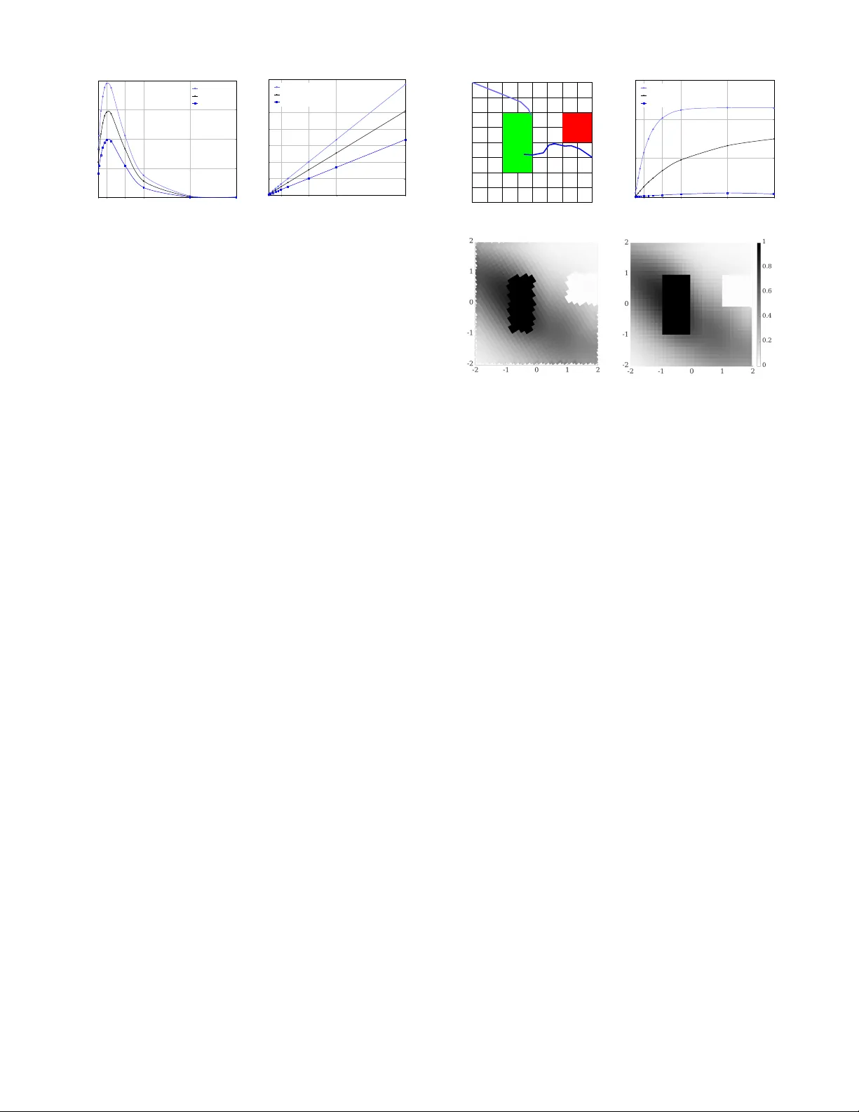
Authors: Nathalie Cauchi, Luca Laurenti, Morteza Lahijanian
Efficiency thr ough Uncer tainty: Scalable Formal Synthesis f or Stochastic Hybrid Systems Nathalie Cauchi, Luca Laurenti, Mor teza Lahijanian, Alessandro Abate, Mar ta Kwiatk owska, and Luca Cardelli ∗ ABSTRA CT This w ork targets the dev elopmen t of an efficien t abstractio n method for formal analysis and contro l syn thesis of discrete- time sto chastic hybrid systems ( shs ) with linear dynamics. The focus is on temporal logic sp ecifications, both o ver finite and infinite time horizons. The framework constructs a finite abstraction as a class of un certain Mark ov models known as interval Markov de cision pr o c ess ( imdp ). Then, a strat- egy that maximizes the satisfaction probabilit y of the given specification is synth esized ov er the imdp and mapped to the underlying shs . In con trast to existing formal approaches, whic h are by and large limited to finite-time prop erties and rely on conserv ative o v er-approximations, w e show that the exact abstraction error can b e computed as a solution of con- v ex optimization problems and can b e embedded into the imdp abstraction. This is later used in the synthesis step o v er b oth finite- and infinite-horizon sp ecifications, mitigat- ing the kno wn state-space explosion problem. Our exp eri- men tal v alidation of the new approach compared to existing abstraction-based approaches shows: (i) significan t (orders of magnitude) reduction of the abstraction error; (ii) mark ed speed-ups; and (iii) bo osted scalability , allowing in particu- lar to v erify models with more tha n 10 con tin uous v ariables. 1. INTR ODUCTION Sto chastic hybrid systems ( shs ) are general and expressiv e models for the quantitativ e description of complex dynami- cal and cont rol systems, suc h as cyb er-ph ysical systems. shs ha v e b een used for mo deling and analysis i n diverse domains, ranging from avionics [1] to chemical reaction net works [2] A CM ISBN 978-1-4503-2138-9. DOI: 10.1145/1235 ∗ L. Lauren ti, M. Lahijanian, A. Abate, L. Cardelli, and M. Kwiatko wsk a are with the Dept. of Computer Science at Univ ersit y of Oxford, U.K. (email: { first- name . lastname } @cs.o x.ac.uk). L. Cardelli is also with Mi- crosoft Research, Cambridge, UK. This work was sup- ported in part by EPSRC Mobile Autonom y Program Grant EP/M019918/1, Roy al Society gran t RP120138, Malta’s ENDEA V OUR sc holarship sc heme and the T uring Institut e, London, UK. and man ufacturing systems [3]. Man y of these applications are safety-critic al ; as a consequence, a theoretical framework pro viding formal guarantees for analysis and control of shs is of ma jor imp ortance. F ormal v erification and synthesis for stochastic pro cesses and shs ha ve been the fo cus of many recen t studies [4– 8]. These methods can provide formal guaran tees on the probabilistic satisfaction of quantitativ e sp ecifications, suc h as those expressed in line ar temp or al lo gic ( l tl ). An ap- proac h to formal verification, whic h is particularly relev ant for discrete-time mo dels, hinges on the abstraction of con- tin uous-space sto chastic mo dels in to discrete-space Mark ov process [4, 6 , 9]. This leads to discrepancies b etw een the ab- stract and original mo dels, whic h can b e captured through error guarantees. The main issue with this approac h is its lac k of scalabilit y to complex mo dels, which is related to t he kno wn state-space explosion problem. This issue is aggra- v ated b y the conserv ative nature of the error b ounds; thus, to guarantee a given v erification error, a v ery fine abstrac- tion is generally required, leading to state-space explosion. This paper introduces a theoretical and computational syn thesis framework for discrete-time shs that is b oth for- mal and scalable. W e zo om in on shs that take the shap e of switc hing diffusions [10], which are linear in the contin uous dynamics and where the con trol action resides in a mo de switc h. W e fo cus on t w o fragmen ts of l tl to enco de prop- erties for the shs , namely co-s afe l tl (cs l tl ) [11], which allo ws the expression of unbounded and complex reachabil- it y prop erties, and b ounde d l tl ( bl tl ) [12], which enables the expression of b ounded-time and safet y prop erties. The framew ork consists of tw o stages (abstraction and control syn thesis) and puts forw ard k ey no vel contri butions. In the first step, (i) we introduce a nov el space discretization tech- nique that is dynamics-dep endent, and (ii) we derive an an- alytical form for tigh t (exact) error b ounds b etw een the ab- straction and the original mo del, (iii) which is reduced to the solution of a set of conv ex optimization problems lead- ing to fast computations. The error is formally em b edded as uncertain transition probabilities in the abstract mo del. In the second stage, (iv) a strategy (control p olicy) is computed b y considering only feasible transition probabilit y distribu- tions ov er the abstract mo del, preven ting the explosion of the error term. Finally , this strategy is soundly refined to a switching strategy for the underlying shs with guarantees on the computed probability bounds. W e provide (v) an illustration of the efficacy of the framework via three case studies, including a comparison with the state of the art. In concl usion, this work pro vides a new computational ab- straction framew ork for discrete-time shs that is b oth formal and mark edly more scalable than s tate-of-the-art tec hniques and to ols. 2. PR OBLEM FORMULA TION W e consider a shs and a property of interest given as a temp oral logic statement. W e are interested in comput- ing a switc hing strategy for this mo del that optimizes the probabilit y of ac hieving the prop erty . Below, we formally in troduce the mo del, prop ert y , and problem. 2.1 Stochastic Hybrid Systems W e conside r a cl ass of discrete-time s hs with linear con tin- uous dynamics and no resets of the contin uous comp onen ts. Definition 1 ( shs ) . A (discr ete-time) line ar sto chastic hy- brid system H is a tuple H = ( A, F , G, Υ , L ) , wher e • A = { a 1 , . . . , a | A | } is a finite set of discr ete mo des, e ach of which c ontaining a c ontinuous domain R m , defining the hybrid state sp ac e S = A × R m , • F = { F ( a ) ∈ R m × m | a ∈ A } is a c ol le ction of drift terms, • G = { G ( a ) ∈ R m × r | a ∈ A } is a c ol le ction of diffusion terms, • Υ = { p 1 , . . . , p n } is a set of atomic pr op ositions, • L : S → 2 Υ is a lab eling function that assigns to ea ch hybrid state p ossibly sever al elements of Υ . A pair s = ( a, x ) ∈ S , where a ∈ A and x ∈ R m , denotes a hybrid state of H , and the evolution of H for k ∈ Z ≥ 0 is a stochastic pro cess s ( k ) = ( a ( k ) , x ( k )) with v alues in S . The term x represen ts the evolution of th e con tin uous component of H according to the sto c hastic difference equation x ( k + 1) = F ( a ) x ( k ) + G ( a ) w, (1) a ∈ A, w ∼ N (0 , C ov w ) , where w is a Gaussian noise with zero mean and cov ariance matrix C ov w ∈ R r × r . The signal a describes the evolution of the discrete modes o ver time. F or κ ∈ Z ≥ 0 ∪ {∞} , w e call Paths κ H : { 0 , 1 , . . . , κ } → S the set of sample paths of s of length κ . The set of all sample paths with finite and infinite lengths are denoted by Paths fin H and Paths H . W e denote by ω H , ω k H , and ω H ( i ) a sample path, a sample path of length k , and the ( i + 1)-th state on the path ω H of H , respectively . Definition 2 (Switc hing strategy) . A switc hing strategy for H is a function σ H : Paths fin H → A that assigns a discr ete mo de a ∈ A to a finite p ath ω H of the pr o c ess s . The set of al l switching str ate gies is denote d by Σ H . Giv en a switching strategy σ H , the evolution of s ( k ) for k < κ , is defined on the probabilit y space ( S κ +1 , B ( S κ +1 ) , P ), where B ( S κ +1 ) is the pro duct sigma-algebra on the pro duct space S κ +1 , and P is a probabilit y measure. W e call T the tr ansition kernel such that for any measurable set B ⊆ R m , x ∈ R m , and a ∈ A , T ( B | x, a ) = Z B N ( t | F ( a ) x, G ( a ) T C ov w G ( a )) dt. (2) Then, it holds that P is uniquely defined b y T , and for k < ∞ , T ( B | x k , a k ) = P ( x ( k + 1) ∈ B | x ( k ) = x k , a ( k ) = a k ) . W e note that, for κ = ∞ , P is still uniquely defined by T b y the Ionescu-T ulc e a extension the or em [13]. W e are interested in the prop erties of H in set ( A × X ) ⊂ S , where X ⊂ R m is a contin uous compact set. Sp ecifically , w e analyze the b ehavio r of H with resp ect to a set of closed regions of interest R = { r 1 , . . . , r n } , where r i ⊆ X . T o this end, we asso ciate to each region r i the atomic proposition (label) p i , i.e., p i ∈ L ( s = ( a, x )) ⇔ x ∈ r i . F urther, we define the (observ ation) trac e of path ω k H = s 0 s 1 . . . s k to b e ξ = ξ 0 ξ 1 . . . ξ k , where ξ i = L ( s i ) ∈ 2 Υ for all i ≤ k . F or a path ω H ∈ Paths H with infinite length, w e obtain an infinite-length trace. 2.2 T emporal Logic Specifications W e employ c o-safe line ar temp or al lo gic (cs l tl ) [11] and b ounde d line ar temp or al lo gic ( bl tl ) [12] to write the prop- erties of H . W e use cs l tl to enco de complex reac habil- it y properties with no time bounds, and bl tl to specify bounded-time properties. Definition 3 (cs l tl syntax) . A cs l tl formula ϕ over a set of atomic pr op osition Υ is inductively define d as fol lows: ϕ : = p | ¬ p | ϕ ∨ ϕ | ϕ ∧ ϕ | X ϕ | ϕ U ϕ | F ϕ, wher e p ∈ Υ , ¬ (ne gation), ∨ (disjunction), and ∧ (c onjunc- tion) ar e Boole an op er ators, and X ( “next” ), U ( “until” ), and F ( “eventual ly” ) ar e temp or al op er ators. Definition 4 ( bl tl syn tax) . A bl tl formula ϕ over a set of atomic pr op osition Υ is inductively define d as fol lowing: ϕ : = p | ¬ ϕ | ϕ ∨ ϕ | X ϕ | ϕ U ≤ k ϕ | F ≤ k ϕ | G ≤ k ϕ, wher e p ∈ Υ is an atomic pr op osition, ¬ (ne gation) and ∨ (disjunction) ar e Bo ole an op er ators, X ( “next” ), U ≤ k ( “b ounde d until” ), F ≤ k ( “b ounde d eventual ly” ), and G ≤ k ( “b ounde d al- ways” ) ar e temp or al op erator s. Definition 5 (Seman tics) . The semantics of cs l tl and bl tl p ath formulas ar e define d over infinite tr ac es over 2 Υ . L et ξ = { ξ i } ∞ i =0 with ξ i ∈ 2 Υ b e an infinite tr ac e and ξ i = ξ i ξ i +1 . . . be the i -th suffix. Notation ξ | = ϕ indic ates that ξ satisfies formula ϕ and is r e cursively define d as fol lowing: • ξ | = p if p ∈ ξ 0 ; • ξ | = ¬ ϕ if ξ 6| = ϕ ; • ξ | = ϕ 1 ∨ ϕ 2 if ξ | = ϕ 1 or ξ | = ϕ 2 ; • ξ | = ϕ 1 ∧ ϕ 2 if ξ | = ϕ 1 and ξ | = ϕ 2 ; • ξ | = X ϕ if ξ 1 | = ϕ ; • ξ | = ϕ 1 U ϕ 2 if ∃ k ≥ 0 , ξ k | = ϕ 2 , and ∀ i ∈ [0 , k ) , ξ i | = ϕ 1 ; • ξ | = F ϕ if ∃ k ≥ 0 , ξ k | = ϕ ; • ξ | = ϕ 1 U ≤ k ϕ 2 if ∃ j ≤ k , ξ j | = ϕ 2 , and ∀ i [0 , j ) , ξ i | = ϕ 1 ; • ξ | = F ≤ k ϕ if ∃ j ≤ k , ξ j | = ϕ ; • ξ | = G ≤ k ϕ if ∀ j ≤ k , ξ j | = ϕ . A trace ξ satisfies a cs l tl or bl tl formula ϕ iff there exists a “go od” finit e prefix ξ of ξ such that the concatenation ξ ξ satisfies ϕ for every suffix ξ [11, 12]. Therefore, even though the semantic s of cs l tl and bl tl are defined ov er infinite traces, we can restrict the analysis to the set of their go o d prefixes, which consists of finite traces. 2.3 Problem Statement W e say that a finite path ω H of H , initialized at state s 0 ∈ S , satisfies a form ula ϕ if the path remains in the compact set X and its corresp onding finite trace ξ | = ϕ . Under a switching strategy σ H , the probabilit y that the shs satisfies ϕ is giv en b y: P ( ϕ | s 0 , X , σ H ) = P ω H ∈ Paths fin ,σ H H | ω H (0) = s 0 , ω H ( k ) ∈ ( A × X ) ∀ k ∈ [0 , | ω H | ] , ξ | = ϕ , (3) where Paths fin ,σ H H denotes the set of all finite paths under strategy σ H , and ξ is the observ ation trace of ω H . In this w ork, we are in terested in synthesizing a switching strategy that maximizes the probabilit y of satisfying prop ert y ϕ . Problem 1 (Strategy synthesis) . Given the shs H in Def. 1, a c ontinuous c omp act set X , and a pr op erty expr esse d as a cs l tl or bl tl formula ϕ , find a switching str ategy σ ∗ H that maximizes the pr ob ability of satisfying ϕ σ ∗ H = arg max σ H ∈ Σ H P ( ϕ | s 0 , X , σ H ) for al l initial states s 0 ∈ A × X . 2.4 Overview of Pr oposed Appr oach W e solve Problem 1 with a discrete abstraction that is both formal and computationally tractable. W e construct a finite model in the form of an uncertain Mark ov pro cess that captures all p ossible b ehaviors of the shs H . This construc- tion in v olv es a discretization of the contin uous set X and hence of R . W e quantify the error of this appro ximation and represen t it in the abstract Marko v model as uncertaint y . W e then syn thesize an optimal strategy on this model that (i) optimizes the probabilit y of satisfying ϕ , (ii) is robust against the uncertaint y and thus (iii) can b e mapp ed (re- fined) onto the concrete mo del H . In the rest of the paper, w e present this solution in detail and sho w all the proofs in Appendix A. 3. PRELIMINARIES 3.1 Marko v Models W e utilize Mark ov mo dels as abstraction structures. Definition 6 ( mdp ) . A Markov de cision pr o c ess ( mdp ) is a tuple M = ( Q, A, P , Υ , L ) , wher e: • Q is a finite set of states, • A is a finite set of actions, • P : Q × A × Q → [0 , 1] is a tr ansition pr ob ability func- tion. • Υ is a finite set of atomic pr op ositions; • L : Q → 2 Υ is a lab eling function assigning to e ach state p ossibly sever al elements of Υ . The set of actions a v ailable at q ∈ Q is denoted by A ( q ). The function P has the prop ert y that P q 0 ∈ Q P ( q , a, q 0 ) = 1 for all pairs ( q , a ), where q ∈ Q and a ∈ A ( q ). A path ω through an mdp is a sequence of states ω = q 0 a 0 − → q 1 a 1 − → q 2 a 2 − → . . . such that a i ∈ A ( q i ) and P ( q i , a i , q i +1 ) > 0 for all i ∈ N . W e denote the last state of a finite path ω fin b y last ( ω fin ) and the set of all finite and infinite paths by Paths fin and Paths , respectively . Definition 7 (Strategy) . A str ate gy σ of an mdp model M is a function σ : Paths fin → A that maps a finite p ath ω fin of M onto an action in A . If a str ate gy dep ends only on last ( ω fin ) , it is c al le d a memoryless or stationary str ate gy. The set of al l str ate gies is denote d by Σ . 1 Giv en a strategy σ , a probability measure Pr ob ov er the set of all paths (under σ ) Paths is induced on the resulting Mark o v chain [16]. A generalized class of mdp s that allows a range of tran- sition probabilities b et w een states is kno wn as b ounde d-p a- r ameter [17] or interval mdp ( imdp ) [18]. Definition 8 ( imdp ) . An interval Markov de cision pr o cess ( imdp ) is a tuple I = ( Q, A, ˇ P , ˆ P , Υ , L ) , wher e Q , A , Υ , and L ar e as in Def. 6, and • ˇ P : Q × A × Q → [0 , 1] is a function, wher e ˇ P ( q , a, q 0 ) defines the lower bound of the tr ansition pr ob ability fr om state q to state q 0 under action a ∈ A ( q ) , • ˆ P : Q × A × Q → [0 , 1] is a function, wher e ˆ P ( q , a, q 0 ) defines the upp er b ound of the tr ansition pr ob ability fr om state q to state q 0 under action a ∈ A ( q ) . F or all q , q 0 ∈ Q and a ∈ A ( q ), it holds that ˇ P ( q , a, q 0 ) ≤ ˆ P ( q , a, q 0 ) and X q 0 ∈ Q ˇ P ( q , a, q 0 ) ≤ 1 ≤ X q 0 ∈ Q ˆ P ( q , a, q 0 ) . Let D ( Q ) denote the set of discrete probabilit y distributions o v er Q . Given q ∈ Q and a ∈ A ( q ), we call γ a q ∈ D ( Q ) a fe asible distribution reachable from q b y a if ˇ P ( q , a, q 0 ) ≤ γ a q ( q 0 ) ≤ ˆ P ( q , a, q 0 ) for each state q 0 ∈ Q . W e denote the set of all feasible distributions for state q and action a b y Γ a q . In imdp s, the notions of paths and strateg ies are extended from those of mdp s in a straigh tforward manner. A distinc- tiv e concept instead is that of adversary , which is a mecha- nism that selects feasible distributions from interv al sets. 2 Definition 9 (Adversary) . Given an imdp I , an adversary is a function π : Paths fin × A → D ( Q ) that, for e ach finite p ath ω fin ∈ Paths fin and action a ∈ A ( last ( ω fin )) , assigns a fe asible distribution π ( ω fin , a ) ∈ Γ a last ( ω fin ) . Giv en a finite path ω fin , a strategy σ , and an adversary π , the semantics of a path of the imdp is as follows. A t state q = last ( ω fin ), first an action a ∈ A ( q ) is chosen by strategy σ . Then, the adversary π resolves the uncertain ties and chooses one feasible distribution γ a q ∈ Γ a q . Finally , the next state q 0 is chosen according to the distribution γ a q , and the path ω fin is extended by q 0 . Giv en a strategy σ and an adv ersary π , a probabili t y mea- sure Pr ob ov er the set of all paths Paths (under σ and π ) is induced by the resulting Marko v c hain [6]. 1 W e fo cus on deterministic strategies as they are suffi- cien t for optimality of cs l tl and bl tl properties [6, 14, 15]. 2 In the verification literature for mdp s, the notions of strategy , p olicy , and adv ersary are often used interc hange- ably . The seman tics of adv ersary o ver imdp s is ho wev er distinguished. 3.2 Polytopes and their P ost Images W e use (conv ex) p olytopes as means of discretization in our abstraction. Let m ∈ N and consider the m -dimensional Euclidean space R m . A full dimensional (conv ex) p olytope P is defined as the con vex h ull of at least m + 1 affinely independent p oints in R m [19]. The set of vertic es of P is the set of p oin ts v P 1 , . . . , v P n P ∈ R m , n P ≥ m + 1, whose con v ex hull gives P and with the prop erty that, for any i = 1 , . . . , n P , p oin t v P i is not in the con vex h ull of the remaining points v P 1 , . . . , v P i − 1 , v P i +1 , . . . , v P n P . A p olytope is completely described b y its set of v ertices, P = c onv ( v P 1 , . . . , v P n P ) , (4) where c onv denotes the conv ex hull. Alternativ ely , P can be describ ed as the b ounded intersection of at least m + 1 closed half spaces. In other words, there exists a k ≥ m + 1, h i ∈ R m , and l i ∈ R , i = 1 , . . . , k such that P = { x ∈ R m | h T i x ≤ l i , i = 1 , . . . , k } . (5) The abov e definition can be written as the matrix inequality H x ≤ L , where H ∈ R k × m and L ∈ R k . Giv en a matrix T ∈ R m × m , the p ost image of p olytope P b y T is defined as [6]: Post (P , T ) = T x | x ∈ P . This post image is a polytop e itself under the linear trans- formation T and can be computed as: Post (P , T ) = c onv {T v P i | 1 ≤ i ≤ n P } . 4. SHS ABSTRA CTION AS AN IMDP As the first step to approac h Problem 1, w e abstract the shs H to an imdp I = ( Q, A, ˇ P , ˆ P , ¯ Υ , L ). Below w e ov erview the construction of the abstraction, and in Sec. 5, we detail the computations inv olved. IMDP States. W e p erform a discretization of the hy- brid state space A × X . F or each discrete mode a ∈ A , w e partition the corresp onding set of in terest X into a set of cells (regions) that are non-o verlapping, except for triv- ial sets of measure zero (their b oundaries). W e assume that each region is a b ounded p olytope. W e denote by Q a = { q a 1 , ..., q a | Q a | } the resulting set of regions in mode a . T o each cell q a i , we associate a state of the imdp I . W e ov er- load the notation by using q a i for b oth a region in X , and a state of I , i.e., q a i ∈ Q . Therefore, the set ( A × X ) ⊂ S can be represented b y ¯ Q = S a ∈ A Q a . The set of imdp states is Q = ¯ Q ∪ { q u } with q u represen ting S \ ( A × X ), namely the complemen t of A × X . IMDP Actions and T ransition Probabilities. W e define the set of actions of I to b e the set of mo des A of H , and allow all actions to b e a v ailable in each state of I , i.e., A ( q ) = A for all q ∈ Q . W e define the one-step transition probabilit y from a con tinuous state x ∈ X to region q ∈ ¯ Q under action (mo de) a ∈ A to b e defined b y the transition k ernel T ( q | x, a ) in (2). The cav eat is that the states of I correspond to regions in H , and there are uncoun tably ma n y possible (contin uous) initial states (here x ) in each region, resulting in a range of feasible transition probabilities to the region q . Therefore, the transition probabilit y from one region to another can be characterized by a range giv en by the min and max of (2) ov er all the p ossible p oints x in the starting region. Thus, we can no w b ound the feasible transition probabilities from state q i ∈ ¯ Q to state q j ∈ ¯ Q from b elo w by γ a q i ( q j ) ≥ min x ∈ q i T ( q j | x, a ) , (6) and from ab ov e by γ a q i ( q j ) ≤ max x ∈ q i T ( q j | x, a ) . (7) Th us, for q i , q j ∈ ¯ Q , we can define the extrema ˇ P and ˆ P of the transition probability of I according to these bounds. Similarly , w e define the b ounds of the feasible transition probabilities to states outside X as γ a q i ( q u ) ≥ 1 − max x ∈ q i T ( X | x, a ) , (8) γ a q i ( q u ) ≤ 1 − min x ∈ q i T ( X | x, a ) , (9) and consequently set the b ounds in I to b e ˇ P ( q i , a, q u ) = 1 − max x ∈ q i T ( X | x, a ) , (10) ˆ P ( q i , a, q u ) = 1 − min x ∈ q i T ( X | x, a ) , (11) for all a ∈ A and q i ∈ ¯ Q . Finally , since we are not in terested in the b eha vior of H outside of A × X , w e render the state q u of I absorbing, i.e., ˇ P ( q u , a, q u ) = ˆ P ( q u , a, q u ) = 1 , ∀ a ∈ A . IMDP Atomic Prop ositions & Labels. In order to en- sure a correct abstraction of H b y I with respect to the lab els of H and the set R = { r 1 , . . . , r n } , ev en for discretizations of A × X that do not resp ect the regions in R , we represent (possibly conserv atively) eac h r i as well as its complement relativ e to X through the lab eling of the states of I . Let r n + i = X \ r i be the complement region of r i with respect to X . W e associate to each r n + i a new atomic prop osition p n + i for 1 ≤ i ≤ n . Intuitiv ely , p n + i represen ts ¬ p i with resp ect to X . W e define the set of atomic propositions for I to b e ¯ Υ = Υ ∪ { p n +1 , . . . , p 2 n } . (12) Then, we design L : Q → 2 ¯ Υ of I such that p i ∈ L ( q ) ⇔ q ⊆ r i , (13) for all q ∈ ¯ Q and 0 ≤ i ≤ 2 n , and L ( q u ) = ∅ . With this modeling, we capture (p ossibly conserv atively) all the prop ert y regions of H by the state labels of I . Then, a formula ϕ o ver Υ of H can be easily translated to a for- m ula ¯ ϕ on ¯ Υ of I by replacing ¬ p i with p n + i . Through this translation, it holds that all the traces that satisfy ¯ ϕ also satisfy ϕ and vice versa. Remark 1. The extension of the atomic pr op ositions in (12) is not ne c essary if the discr etization of A × X r esp e cts al l the r e gions in R , i.e., ∃ Q r ⊆ Q s.t. ∪ q ∈ Q r q = r for al l r ∈ R . 5. COMPUT A TION OF THE IMDP In this section, w e introduce an efficient and scalable method for space discretization and computation for min x ∈ q i T ( q j | x, a ) , max x ∈ q i T ( q j | x, a ) . (14) T o this end, we first define a hyp er-r ectangle and pr oper tr anformation function as follows. Definition 10 (Hyper-rectangle) . A hyp er-r ecta ngle in R m is an m -dimensional r e ctangle define d by the intervals [ v (1) l , v (1) u ] × [ v (2) l , v (2) u ] × · · · × [ v ( m ) l , v ( m ) u ] , (15) wher e vectors v l , v u ∈ R m c aptur e the lower and upp er values of the vertic es of the r ectangle in e ach dimension, and v ( i ) denotes the i -th comp onent of ve ctor v . Definition 11 (Prop er transformation) . F or a p olytop e q ⊂ R m , the tr ansformation function T ∈ R m × m is pr op er if Post ( q , T ) is a hyp er-r e ctangle. W e also note that pro cess x in mo de a is Gaussian with one-step cov ariance matrix C ov x ( a ) = G ( a ) T C ov w G ( a ) . (16) Then, we can characterize T ( q | x, a ) analytically as follows. Prop osition 1. F or pr oc ess x in mo de a ∈ A , let T a = Λ − 1 2 a V T a b e a tr ansformation function (matrix), wher e Λ a = V T a C ov x ( a ) V a is a diagonal matrix whose entries ar e eigen- values of C ov x ( a ) and V a is the c orr esp onding orthonormal (eigenve ctor) matrix. F or a p olytopic re gion q ⊂ R m , if T a is pr op er, then it holds that T ( q | x, a ) = 1 2 m m Y i =1 erf ( y ( i ) − v ( i ) l √ 2 ) − erf ( y ( i ) − v ( i ) u √ 2 ) , (17) wher e erf ( · ) is the erro r function, and y ( i ) is the i -th c om- p onent of ve ctor y = T a F ( a ) x , and v ( i ) l , v ( i ) u ar e as in (15) . A direct consequence of Prop osition 1 is that the opti- mizations in (14) can be performed on (17) through a proper transformation, as stated b y the following corollary . Corollary 1. F or p olytopic r e gions q i , q j ⊂ R m and pr o c ess x in mo de a , assume T a is a pr op er tr ansformation function with r esp e ct to q j , and define q 0 i = Post ( q i , F ( a )) and f ( y ) = 1 2 m m Y i =1 erf ( y ( i ) − v ( i ) l √ 2 ) − erf ( y ( i ) − v ( i ) u √ 2 ) , (18) wher e v l and v u ar e as in (15) . Then, it holds that min x ∈ q i T ( q j | x, a ) = min y ∈ Post ( q 0 i , T a ) f ( y ) , max x ∈ q i T ( q j | x, a ) = max y ∈ Post ( q 0 i , T a ) f ( y ) . The ab ov e prop osition and corollary show that, for a par- ticular prop er transformation function T a , an analytical form can b e obtained for the discrete kernel of the imdp . This is an imp ortan t observ ation b ecause it enables efficien t com- putation for the min and max v alues of the kernel. There- fore, we use a space discretization to satisfy the condition in Proposition 1 as describ ed b elow . 5.1 Space Discretization F or each mo de a ∈ A , we define the linear transformation function (matrix) of T a = Λ − 1 2 a V T a , (19) where Λ a = V T a C ov x ( a ) V a is a diagonal matrix whose en- tries are the eigen v alues of C ov x ( a ), and V a is the corre- sponding orthonormal (eigenv ector) matrix. The discretiza- tion of the contin uous set X in mo de a is achiev ed by using a grid in the transformed space by T a . That is, w e first transform X b y T a , and then discretize it using a grid. This method of discretization guaran tees that, for eac h q a ∈ Q a , Post ( q a , T a ) is a h yp er-rectangle, i.e., T a is prop er. Hence, w e can use the result of Prop osition 1 and Corollary 1 for the computation of the v alues in (14). Remark 2. F or an arbitr ary geo metry of X , it may not b e p ossible to obtain a discr etization such that S q a ∈ Q a q a = X . Nevertheless, by using a discr etization that under-appr oxima tes X , i.e., S q a ∈ Q a q a ⊆ X , in e ach mo de a , we can c ompute a lower b ound on the pr obab ility of satisfaction of a given pr op erty ϕ . F or a b etter appr oximation, the grid c an b e non- uniform, al lowing in p articular for smal ler c el ls ne ar the b oundary of X , as in [4]. 5.2 T ransition Probability Bounds W e distinguish betw een transitions from q ∈ ¯ Q to the states in ¯ Q and to the state q u . 5.2.1 T ransitions to q ∈ ¯ Q W e present tw o approaches to solving the v alues for (14). The first approach is based on Karush-Kuhn-T ucker ( kkt ) conditions [20], which sheds ligh t into the optimization prob- lem and lay s down the conditions on where to look for the op- timal p oints, giving geometric intuition. This method boils do wn to solving systems of non-linear equations, which turns out to be efficien t and exact for lo w-dimensional systems. In the second approac h, we sho w that the problem reduces to a conv ex optimization problem, allowing the adoption of ex- isting optimization tools and hence making the approac h suitable for high-dimensional systems. KKT Optimization Approac h: In the next theorem, w e use the result of Corollary 1 and the kkt conditions [20] to compute the exact v alues for (14). Theorem 1. F or p olytopic r e gions q i , q j ⊂ R m and pr oper tr ansformation matrix T a with r esp e ct to q j , let Post ( q 0 i , T a ) = { y ∈ R m | H y ≤ b } , wher e q 0 i = Post ( q i , F ( a )) , H ∈ R k × m , b ∈ R m , and k ≥ m + 1 , and intr o duc e the fol lowing c onditions: • Condition 1 : y is at the center of Post ( q j , T a ) , i.e., y = ( v (1) u + v (1) l 2 , . . . , v ( m ) u + v ( m ) l 2 ) . • Condition 2 : y is a vertex of Post ( q 0 i , T a ) . • Condition 3 : y is on the b oundary of Post ( q 0 i , T a ) , wher e r ≥ 1 of the k half-sp ac es that define Post ( q 0 i , T a ) interse ct, and ∇ f ( y ) = ¯ H T µ, for ve ctor µ = ( µ 1 , . . . , µ r ) of non-ne gative c onstants, and submatrix ¯ H ∈ R r × m that c ontains only the r ows of H that c orr esp ond to the r -interse cting half-sp ac es at y . • Condition 4 : y is as in Condition 3 , and ∇ f ( y ) = − ¯ H T µ, for ve ctor µ = ( µ 1 , . . . , µ r ) of non-ne gative c onstants, and ¯ H is define d as in Condition 3 . Then, it fol lows that the p oint y ∈ Post ( q 0 i , T a ) that satis- fies Condition 1 ne c essarily maximizes f ( y ) . If Condition 1 c annot be satisfie d, then the maximum is ne c essarily given by one of the p oints that satisfy Condition 2 or 3 . F urthermor e, the poi nt y ∈ Post ( q 0 i , T a ) that minimizes f ( y ) nec essarily satisfies Condition 2 or 4 . Theorem 1 iden tifies the argumen ts (p oin ts y ∈ Post ( q 0 i , T a )) that give rise to the optimal v alues of T in (14). Then, the actual optimal v alues of T can b e computed by (18) as guaranteed b y Corollary 1. Therefore, from Theorem 1, an algorithm can b e constructed to generate a set of finite candidate p oints based on Conditions 1-4 and to obtain the exact v alues of (14) by plugging those p oints into (18). In short, Condition 1 maximizes the unconstrained prob- lem and giv es rise to the global maximum. Hence, if the cen ter of q j is con tained in Post ( q 0 i , T a ), no further c hec k is required for maximum. If not, the maxim um is given b y a point on the boundary of Post ( q 0 i , T a ). It is either a vertex (Condition 2) o r a boundary poin t that sati sfies Condition 3. The minimum is alwa ys giv en by a boundary p oin t, which can b e either a vertex or a b oundary p oin t that satisfies Condition 4. Note that Conditions 3 and 4 are similar and both state that the optimal v alue of T is given by a p oin t where the gradien t of T becomes linearly dep enden t on the v ectors that are defined by the intersecting half-spaces of Post ( q 0 i , T a ) at that point. Each of these tw o conditions de- fines a system of m equations and r < m v ariables, which ma y hav e a solution only if some of the equations are linear com binations of the others. The ab o ve algorithm computes the exact v alues for the transition probability b ounds. It is com putationally efficient for small dimensional systems, e.g., m < 4. F or large m , ho w ev er, the efficiency drops b ecause the num b er of b ound- ary constraints that need to b e chec ked and solv ed for in Conditions 3 and 4 increases, in the worst case, exponen- tially with m . Belo w, w e prop ose an equiv alent but more efficien t metho d to compute min and max of T for large dimensional systems, e.g., m ≥ 4. Con vex Optimization Approach: In order to show ho w upp er and low er b ounds of f ( y ) can b e efficiently com- puted using con vex optimization tools, we need to in tro duce the definition of c onc ave and lo g-c onc ave functions. Definition 12 (Conca ve F unction) . A function g : R m → R is said to b e c onc ave if and only if for y 1 , y 2 ∈ R m , λ ∈ [0 , 1] g ( λy 1 + (1 − λ ) y 2 ) ≥ λg ( y 1 ) + (1 − λ ) g ( y 2 ) . Definition 13 (Log-conca ve F unction) . A function g : R m → R is said to b e lo g-c onc ave if and only if log ( g ) is a c onc ave function. That is, for y 1 , y 2 ∈ R m , λ ∈ [0 , 1] g ( λy 1 + (1 − λ ) y 2 ) ≥ g ( y 1 ) λ g ( y 2 ) (1 − λ ) . In the followi ng proposition, we show that f ( y ), as defined in Corollary 1, is log-conca v e. This enables efficien t computa- tion of the upp er and lo wer b ounds of f ( y ) through standard con v ex optimization techniques such as gradient descent or semidefinite programming [21]. Hence, we can mak e use of readily av ailable softw are to ols, e.g., NLopt [22], which ha v e been highly optimized in terms of efficiency and scalabilit y . Prop osition 2. f ( y ) , as define d in Cor ol lary 1, is a lo g- c onc ave function. 5.2.2 T ransitions to sink state q u Here, we fo cus on the transition probabilities to state q u in (10) and (11). T o this end, w e need to compute max x ∈ q i T ( X | x, a ) , min x ∈ q i T ( X | x, a ) . (20) W e can efficiently compute b ounds for these quantities by using the results obtained ab ov e. The following prop osition sho ws this efficient metho d of computation. Prop osition 3. L et ˇ Q a and ˆ Q a b e two sets of p olytopic r e gions in mo de a such that [ q ∈ ˇ Q a q ⊆ X ⊆ [ q ∈ ˆ Q a q , and T a b e a pr op er tr ansformation function for every q ∈ ˇ Q a ∪ ˆ Q a , and c al l f ( y , q ) = 1 2 m m Y i =1 erf ( y ( i ) − v ( i ) l,q √ 2 ) − erf ( y ( i ) − v ( i ) u,q √ 2 ) , (21) wher e v l,q and v u,q ar e as in (15) for q . Then, it holds that max x ∈ q i T ( X | x, a ) ≤ max y ∈ Post ( q 0 i , T a ) X q ∈ ˆ Q a f ( y , q ) , (22) min x ∈ q i T ( X | x, a ) ≥ min y ∈ Post ( q 0 i , T a ) X q ∈ Q a f ( y , q ) , (23) wher e q 0 i = Post ( q i , F ( a )) . In tuitiv ely , Proposition 3 states that, with a particular c hoice of discretization, i.e., a grid in the transformed space, the transition probability to X is equal to the sum of the transition probabilities to the discrete regions, where each discrete transition kernel is given by the close-form function f ( y , q ) in (21). If X cannot b e precisely discretized with a grid (in the transformed space), then the upp er and low er bounds of the transition probabilities are given by the ov er- and under-approximat ing grids ( ˆ Q a and ˇ Q a ), resp ectiv ely . Remark 3. F or the computat ion of the values in (22) and (23) , Pr op osition 2 c an b e applie d, making b oth metho ds of kkt and c onvex optimization applic able. 6. STRA TEGY SYNTHESIS AS A GAME Recall that our ob jectiv e is, given the compact set X and a bl tl or cs l tl formula ϕ , to compute a strategy for H that maximizes the probability of satisfying ϕ without exiting X . The imdp abstraction I , as constructed ab ov e, captures (possibly conserv ativ ely) the b eha vior of the shs H with respect to the regions of interest R within X , and the prob- abilities of exiting X are enc ompassed via the state q u . Since state q u is absorbing, the paths of I are not allow ed to exit and re-enter X ; as such, the analysis on I narrows the fo cus to dynamics within set X , as desired. Therefore, w e can focus on finding a strategy for I that is robust against all the uncertain ties (errors) introduced by the discretizatio n of A × X and which maximizes ϕ . The uncertainties in I can b e viewed as the nondetermin- istic c hoice of a feasible transition probabilit y from one imdp state to another under a giv en action. Therefore, w e in ter- pret a synthesis task ov er the imdp as a 2-play er sto c hastic game, where Play er 1 c hooses an action a ∈ A at st ate q ∈ Q , and Play er 2 chooses a feasible transition probability distri- bution γ a q ∈ Γ a q . T o wards robust analysis, we set up this game as adversarial: the ob jectives of Play ers 1 and 2 are to maximize and minimize the probabilit y of satisfying ϕ , re- spectively . Hence, the goal b ecomes to synthesize a strategy for Pla yer 1 that is robust against all adversari al choices of Pla y er 2 and maximizes the probability of ac hieving ϕ . In order to compute this strategy , we fi rst translate ϕ ov er Υ into its equiv alent formula ¯ ϕ ov er ¯ Υ. Then, we construct a deterministic finite automaton ( df a ) A ¯ ϕ that precisely accepts all the goo d prefixes that satisfy ¯ ϕ [11]. Definition 14 ( df a ) . A df a c onstructe d fr om a cs l tl or bl tl formula ¯ ϕ is a tuple A ¯ ϕ = ( Z , 2 ¯ Υ , τ , z 0 , Z ac ) , wher e Z is a finite set of states, 2 ¯ Υ is the set of input alphab ets, τ : Z × 2 ¯ Υ → Z is the tra nsition function, z 0 ∈ Z is the initial state, and Z ac ⊆ Z is the set of ac c epting states. A finite run of A ¯ ϕ on a trace ξ = ξ 1 · · · ξ n , where ξ i ∈ 2 ¯ Υ , is a sequence of states µ = z 0 z 1 . . . z n with z i = τ ( z i − 1 , ξ i ) for i = 1 , . . . , n . Run µ is called acc epting if µ n ∈ Z ac . T race ξ | = ¯ ϕ iff its corresp onding run µ in A ¯ ϕ is accepting. Next, we construct the product imdp I ¯ ϕ = I × A ¯ ϕ , which is a tuple I ¯ ϕ = ( Q ¯ ϕ , A ¯ ϕ , ˇ P ¯ ϕ , ˆ P ¯ ϕ , Q ¯ ϕ ac ), where Q ¯ ϕ = Q × Z, A ¯ ϕ = A, Q ¯ ϕ ac = Q × Z ac , ˇ P ¯ ϕ (( q , z ) , a, ( q 0 , z 0 )) = ( ˇ P ( q , a, q 0 ) if z 0 = τ ( z , L ( q 0 )) 0 otherwise , ˆ P ¯ ϕ (( q , z ) , a, ( q 0 , z 0 )) = ( ˆ P ( q , a, q 0 ) if z 0 = τ ( z , L ( q 0 )) 0 otherwise , for all q , q 0 ∈ Q , a ∈ A , and z ∈ Z . In tuitively , I ¯ ϕ con tains both I and A ¯ ϕ and hence can iden tify all the paths of I that satisfy ¯ ϕ , i.e., the satisfying paths terminate in Q ¯ ϕ ac since their corresp onding A ¯ ϕ runs are accepting. Therefore, the syn thesis problem reduces to computing a robust strategy on I ¯ ϕ that maximizes the probability of reac hing Q ¯ ϕ ac . This problem is equiv alen t to solving the maximal r e achability pr ob ability pr oblem [6, 23] as explained b elo w. Giv en a strategy σ on an imdp , the probabilit y of reac hing a terminal state from each state is necessarily a range for all the a v ailable adversarial choices of Pla y er 2. Let ˇ p σ ( q ) and ˆ p σ ( q ) denote lo wer and upp er b ounds for the probabilit y of reaching a state in Q ¯ ϕ ac starting from q ∈ Q ¯ ϕ under σ . Deriv ed from the Bellman equation, we can compute the optimal low er b ound by recursive ev aluations of ˇ p σ ∗ ( q ) = 1 if q ∈ Q ¯ ϕ ac max a ∈ A ( q ) min γ a q ∈ Γ a q P q 0 ∈ Q ¯ ϕ γ a q ( q 0 ) ˇ p σ ∗ ( q 0 ) otherwise, (24) for all q ∈ Q ¯ ϕ . Eac h iteration of this Bellman equation in v olv es a minimization o v er the adv ersarial c hoices, which can b e computed through an ordering of the states of I ¯ ϕ [6, 17], and a maximization ov er the actions. This Bellman equation is guaran teed to con v erge in finite time [6, 23] and results in the lo wer-bound probabilit y ˇ p σ ∗ ( q ) for each q ∈ Q ¯ ϕ and in a stationary (memoryless) strategy σ ∗ . The upp er bounds are similarly given by recursive ev aluations of ˆ p σ ∗ ( q ) = 1 if q ∈ Q ¯ ϕ ac max γ σ ∗ q ∈ Γ σ ∗ q P q 0 ∈ Q ¯ ϕ γ σ ∗ q ( q 0 ) ˆ p σ ∗ ( q 0 ) otherwise, (25) whic h is also guaran teed to con v erge in finite time. The optimal strategy σ ∗ on I ¯ ϕ can b e mapped onto the states and actions of the abstraction imdp I , resulting in a (history-dep endent) strategy . By construction, then the optimal low er and upp er probability b ounds of satisfying ϕ from the states of I are: ˇ p σ ∗ ϕ ( q ) = ˇ p σ ∗ (( q , z 0 )) , ˆ p σ ∗ ϕ ( q ) = ˆ p σ ∗ (( q , z 0 )) , (26) for all q ∈ Q of I . The complexity of the ab ov e strategy synthesis algorithm is p olynomial in the size of the imdp I ¯ ϕ [6, 23] and exp o- nen tial in the size of the formula ϕ (in the w orst case) [11]. Note that the size of ϕ used to express the prop erties of shs is typically small. 7. CORRECTNESS W e show that the strategy σ ∗ computed ov er I can b e re- fined ov er (mapped onto) H and the low er probabilit y bound ˇ p σ ∗ ϕ on I alw a ys holds for the h ybrid system H . The upper bound ˆ p σ ∗ ϕ also holds for H if the discretization respects the regions in R . In the case that the discretization is not R - respecting, a mo dified upp er b ound that holds for H can b e computed with a small additional step as detailed b elow. Let : S → Q be a function that maps the hybrid states s ∈ S to their corresp onding discrete regions (states of I ), i.e, ( s ) = q ∈ Q if s ∈ q . With a sligh t abuse of notations, w e also use to denote the mapping from the finite paths of H to their corresponding paths of I , i.e., ω k H = s 0 s 1 . . . s k ⇒ ( ω k H ) = ( s 0 )( s 1 ) . . . ( s k ) . Then, the imdp strategy σ ∗ correctly maps to a switching strategy σ ∗ H for H via σ ∗ H ( ω k H ) = σ ∗ (( ω k H )) . (27) The follo wing theorem sho ws that for a given ϕ , the prob- abilit y bounds ˇ p σ ∗ ϕ and ˆ p σ ∗ ϕ are guaran teed to hold for the process s under σ ∗ H as constructed ab ov e. Theorem 2. Given a shs H , a c ontinuous set X , and a cs l tl or bl tl formula ϕ , let I b e the imdp abstr action of H as describ e d in Se ction 4 thr ough a discr etization that r esp e cts the r e gions of inter est in R . F urther, let σ ∗ b e the str ate gy on I c ompute d by (24) and (25) with pr ob ability b ounds ˇ p σ ∗ ϕ and ˆ p σ ∗ ϕ in (26) . R efine σ ∗ into a switching str ate gy σ ∗ H as in (27) . Then, for any initial hybrid state s 0 ∈ S , wher e s 0 ∈ q 0 ∈ Q , it holds that P ( ϕ | s 0 , X , σ ∗ H ) ∈ ˇ p σ ∗ ϕ ( q 0 ) , ˆ p σ ∗ ϕ ( q 0 ) . (28) Note that an assumption in Theorem 2 is that the dis- cretization Q resp ects the regions in R . If this assumption is violated, then the lo wer bound ˇ p σ ∗ ϕ still holds, unlike the upper b ound ˆ p σ ∗ ϕ . That is b ecause we design the lab eling function L of I to under-approximate the regions of interest r ∈ R , making the upp er b ound ˆ p σ ∗ ϕ v alid with resp ect to the under-appro ximate represen tation of R b y L but p ossi- bly under-approximated with resp ect to the actual R . T o compute an upp er b ound that accounts for this, we need to design a new lab eling function that ov er-appro ximates the labels of each region, as follows . Let L 0 : Q → ¯ Υ b e this labeling function with p i ∈ L 0 ( q ) ⇔ ∃ ( a, x ) ∈ q s.t. x ∈ r i , (29) where p i ∈ ¯ Υ is the asso ciated prop osition to r i ∈ R . Then, w e can compute the o ver-appro ximated upper bound ˆ p 0 σ ∗ ϕ via (25) on the pro duct imdp I 0 ¯ ϕ constructed using L 0 . Lemma 1. If abstr action I is c onstructe d thr ough a dis- cr etization that do es not r esp e ct the r e gions in R , then P ( ϕ | s 0 , X , σ ∗ H ) ∈ ˇ p σ ∗ ϕ ( q 0 ) , ˆ p 0 σ ∗ ϕ ( q 0 ) , (30) wher e ˆ p 0 σ ∗ ϕ is c ompute d via (25) using the lab els in (29) . Theorem 2 and Lemma 1 guarantee that the satisfaction probabilit y of ϕ for the pro cess s , solution of the shs H , is con tained in the probability in terv al computed on the ab- straction I . The size of this interv al dep ends on the differ- ence of the one-step transition probability b ounds of ˇ P and ˆ P as well as the embedded approximations in the lab eling functions L and L 0 in I , which can be viewed as the error in- duced by space discretization of H cast into the abstraction I . This error can b e tuned by the size of the discretization: in particular, in the limit of an infinitely fine grid, the error of the abstraction goes to zero, and the imdp abstraction is refined in to an mdp , namely for all q, q 0 ∈ Q and a ∈ A ( q ), ˇ P ( q , a, q 0 ) → P ( q , a, q 0 ) ← ˆ P ( q , a, q 0 ). Remark 4. In pra ctic e, the inter est in synthesis pr oblems is typic al ly on deriving lower b ounds for the pr ob ability, wher e as the upp er b ound c omputation is useful for err or analysis. Remark 5. With a simple mo dific ation, the pr op ose d fr ame- work c an b e use d for verific ation of shs H against pr op- erty ϕ : (i) c ompute the lower-b ound pr obabi lity by r eplac- ing max a ∈ A ( q ) with min a ∈ A ( q ) in (25) on abstr action I with lab eling function L , and (ii) c ompute the upp er-b ound pr ob- ability by r eplacing min γ a q ∈ Γ a q with max γ a q ∈ Γ a q in (25) on ab- str action I with lab eling function L 0 . 8. EXPERIMENT AL RESUL TS W e implement the abstraction and synthesis algorithms and test their performance on three case studies. W e first presen t a tw o dimensional sto c hastic pro cess with a single mode and p erform a comparison against the algorithms and tool f aust 2 [24] in Case Study 1. Next, we consider a t wo dimensional, tw o-mo de mo del and sho w the synthesis o ver un bounded-time prop erties in Case Study 2. Last, we ana- lyze the scalability of the proposed techniques ov er increas- ing contin uous dimension of the shs in Case Study 3. The implementatio n of the abstraction algorithm is in ma tlab and c++ : more precisely , the approach based on kkt method is in ma tlab (as a pro of of concept), and the con v ex optimization metho d with gr adient de c ent ( gd ) is in c++ . The synthesis algorithm ov er the imdp is also imple- men ted in c++ . The exp eriments are run on an In tel Core i7-8550U CPU at 1.80GHz × 8 machine with 8 GB of RAM. 8.1 Case Study 1 - F ormal V erification W e consider a stochastic p rocess with dynamics in (1) and a single discrete mode ( A = { a 1 } ), where F ( a 1 ) = 0 . 85 0 0 0 . 90 , G ( a 1 ) = 0 . 15 0 0 0 . 05 , with X = [ − 1 , 1] × [ − 1 , 1] and safety prop ert y ϕ 1 = G ≤ k X. W e compare the verification results of the ab ov e model using our method against those of the state-of-the-art tool f aust 2 [24]. Namely , we compare probability of satisfaction of ϕ 1 , computation times, and errors for a range of v alues for time horizon k and grid sizes. T o obtain the imdp abstrac- tion of our metho d, we used a uniform gri d discretization per Sec. 5. T ool f aust 2 abstracts the model into an mdp and treats the error as a separate parameter. The grid generated in f aust 2 is based on computation of the global Lipsc hitz constan t via in tegrals [24]. W e define the error of the imdp method to b e ε q = ˆ p ∗ ϕ ( q ) − ˇ p ∗ ϕ ( q ) for each state, and the global error to be ε max = max q ∈ Q ε q . Similarly , for f aust 2 the resulting error corresponds to the maximum error ov er all the states. The f a ust 2 tool is written in ma tlab and run o v er this platform, how ever additionally for fair comparison w e hav e re-implemen ted the abstraction based on f aust 2 in the c++ language (cf. corresp onding lines in T able 1). The results are show n in T able 1 for k = 2 and v arious grid sizes. W e saturate conserv ative errors output b y f aust 2 that are greater than 1 to this v alue. F or the particular grid | Q | = 3722, the lo wer bound probabilities of satisfying ϕ 1 are shown in Fig. 3 within App endix B. As evident in T able 1, our approac h greatly outp erforms the state of the art. With resp ect to the error generated for the same grid size, our metho d has significantly (an order of magnitude) smaller error than f aust 2 . Our imdp metho d also requires lo w er computation times. W e also note that, as guaranteed b y the theory (Theorem 1 and Proposition 2), both kkt and gd approaches compute the same error. T o ol Impl. | ¯ Q | Time tak en Error Method Platform (states) (secs) ε max imdp ( kkt ) ma tlab 361 19.789 0.211 imdp ( gd ) c++ 361 29.003 0.211 f aust 2 ma tlab 361 108.265 1.000 f aust 2 c++ 361 136.71 1.000 imdp ( kkt ) ma tlab 625 145.563 0.163 imdp ( gd ) c++ 625 117.741 0.163 f aust 2 ma tlab 625 285.795 1.000 f aust 2 c++ 625 302.900 1.000 imdp ( kkt ) ma tlab 1444 4464.78 3 0.109 imdp ( gd ) c++ 1444 510.920 0.109 f aust 2 ma tlab 1444 1445.441 1.000 f aust 2 c++ 1444 1201.950 1.000 imdp ( kkt ) ma tlab 2601 28127.256 0.082 imdp ( gd ) c++ 2601 2939.050 0.082 f aust 2 ma tlab 2601 5274.578 0.995 f aust 2 c++ 2601 3305.490 0.995 imdp ( kkt ) ma tlab 3721 Time out 3 - imdp ( gd ) c++ 3721 3973.28 0.068 f aust 2 ma tlab 3721 11285.313 0.832 f aust 2 c++ 3721 7537.750 0.832 T able 1: Comparison of verification results of our imdp al- gorithms against f aust 2 for ϕ 1 with k = 2. In Fig. 1, we show the error of each metho d as a function of the time horizon k in ϕ 1 . F rom these figures it is evident that our approac h again greatly outp erforms f aust 2 . That is b ecause our metho d embeds the error in the abstraction and performs computations according to feasible transition probabilities, whic h prev en ts the error from explo ding o ver time, whereas the error of f aust 2 k eeps increasing mono- tonically with the time horizon. An interesting asp ect in 1 10 30 50 100 ∞ 0 0.1 0.2 0.3 0.4 Time Horizon ( k ) IMDP Error ( ǫ max ) | ¯ Q | = 361 | ¯ Q | = 625 | ¯ Q | = 1444 2 (a) imdp 1 10 30 50 100 0 20 40 60 80 100 Time Horizon ( k ) F AUST 2 Error ( ǫ max ) | ¯ Q | = 361 | ¯ Q | = 625 | ¯ Q | = 1444 4 (b) f aust 2 Figure 1: Maximum error incurred in satisfying ϕ 1 as a function of time horizon k . Fig. 1a is that the error of our metho d goes to zero as k increases. That is because the system under consideration is an unbounded Gaussian pro cess, and despite its stable dy- namics, the probability of it remaining within the b ounded set X approaches zero as time grows larger. This is mean- ingfully captured b y b oth the upp er and lo wer probabilit y bounds of our metho d. On the other hand, f a ust 2 is not able to capture this b eha vior and its error explo des. 8.2 Case Study 2 - Strategy synthesis W e consider a 2-dimensional shs with tw o modes A = { a 1 , a 2 } : F ( a 1 ) = 0 . 1 0 . 9 0 . 8 0 . 2 , G ( a 1 ) = 0 . 3 0 . 1 0 . 1 0 . 2 , F ( a 2 ) = 0 . 8 0 . 2 0 . 1 0 . 9 , G ( a 2 ) = 0 . 2 0 0 0 . 1 . Note that F ( a 1 ) and F ( a 2 ) are not asymptotically stable, as they both hav e one eigenv alue equal to 1. W e are inter- ested in syn thesizing a switc hing strategy that maximizes the probability of satisfying ϕ 2 = ¬ r ed U g r een. within the set X = [ − 2 , 2] × [ − 2 , 2]. The regions asso ciated with the lab els r e d and gr een are depicted in Fig. 2a. Note that ϕ 2 has an un bounded time horizon, hence, f aust 2 cannot b e applied. W e make use of an adaptive grid, in- spired b y [4], such that the resulting cells hav e maximum and minimum sizes in the original space of ∆ x max = 0 . 13 and ∆ x min = 0 . 05, respectively . Our adaptiv e-grid algo- rithm first o ver-appro ximates Post ( X , T a i ) for i ∈ { 1 , 2 } b y using a uniform grid with the allow ed maximum-sized cells. It refines the cells that b elong to th e green and red regions in the original space, up to the resolution of the minim um-sized cells. Fig. 2c and 2d show the discretizatio n of mo des a 1 and a 2 , respectively . The generated imdp has | Q | = 3612 states with | Q a 1 | = 1862 and | Q a 2 | = 1750. Note that in mo de a 1 the cells associated with the label ¬ r ed under-appro ximate X \ r ed , i.e., the red region is ov er-approxi mated, whereas the regions asso ciated with the lab el gr e en under-appro ximate the green region. This is due to the transformation function T a 1 , which includes a rotation in addition to a translation, whic h do es not resp ect the regions of in terest in R . W e run the syn thesis algori thm to obtain the robust strat- egy σ ∗ ϕ 2 with the corresp onding low er probability b ounds. F or each state, the lo w er probability b ounds are depicted in gre en r ed gre en -2 -1 0 2 1 -2 -1 0 1 2 (a) 1 10 30 50 100 ∞ 0 0.1 0.2 0.3 Time Horizon ( k ) IMDP Error ( ǫ max ) | ¯ Q | = 874 | ¯ Q | = 1400 | ¯ Q | = 3612 3 (b) (c) (d) Figure 2: Syn thesis results for ϕ 2 with (a) original set X with sim ulated tra jectories under σ ∗ ϕ 2 , (b) maxim um error incurred in satisfying ϕ 2 as function of time horizon k , and lo w er b ound probabilities of satisfying ϕ 2 for mo des (c) a 1 and (d) a 2 . Fig. 2c and 2d. The total time to compute the abstraction and to generate σ ∗ ϕ 2 is 5434 seconds. Fig. 2a shows the sim- ulation of tw o tra jectories using σ ∗ ϕ 2 with a starting p oint of (2 , − 0 . 5) within mo de a 1 and ( − 2 , 2) within mode a 2 re- spectively . In both instances, the property ϕ 2 is satisfied. W e also analyze the errors of our method for ϕ 2 as a func- tion of time horizon for v arious grid sizes. Fig. 2b shows the results. It can b e seen that, for a fixed k , ε max decreases monotonically with the num b er of states (similar to Fig. 1a in Cas e Stu dy 1), and ε max con v erges to a steady-state v alue for each grid size as the time horizon increases. 8.3 Case Study 3 - Scaling in continuous di- mension W e consider a sto chastic process with A = { a 1 } (single mode) and dynamics characterised by F ( a 1 ) = − 0 . 95 I d and G ( a 1 ) = 0 . 1 I d , where d corresp onds to the contin uous di- mension of the stochastic process (num b er of contin uous v ariables) and X = [ − 1 , 1] d . W e are in terested in chec k- ing the sp ecification ϕ 3 = G ≤ 50 X as the conti n uous dimension d of the mo del v aries. W e use a uniform grid characterized by parameter ∆ x = 1 per side. W e compute the corresponding lo w er- and upp er- bound probabilities of satisfying ϕ 3 and list the num ber of states required for each dimension together with the asso ci- ated ε max in T able 2. The method generates abstract mo dels with manageable state spaces, and displays scalability with respect to the contin uous dimension d of the shs to mo dels with more than ten v ariables, which is a marked impro v e- men t ov er state-of-the-art to ols [24]. Dimensions | ¯ Q | Time taken Error (d) (states) (secs) ( ε max ) 2 4 0.014 0.030 3 14 0.088 0.003 4 30 0.345 0.004 5 62 1.576 0.003 6 125 6.150 0.004 7 254 23.333 0.003 8 510 88.726 0.003 9 1022 367.133 0.003 10 2046 1787.250 0.003 11 8190 25500.000 0.003 T able 2: V erification results of our imdp approach for ϕ 3 . 9. CONCLUSIONS This work has presen ted a theoretical and computational tec hnique for a nalysis and synthesis of discrete-time stochas- tic h ybrid systems. A suitable c hoice of the abstraction framew ork results in exact error bounds, leading to precise and compact abstractions for the synthesis tasks. The ex- perimental results illustrate that the prop osed framework greatly outp erforms the state of the art time-wise and that is more scalable, thus mitigating the state-space explosion problem. Whilst the framework is tailored to bl tl and cs l tl properties, it can b e extended to v erification and syn thesis for more complex and even multi-ob jectiv e [18] prop erties. 10. REFERENCES [1] H. Blom and J. Lygeros (Eds.), Sto chastic Hybrid Systems: The ory and Safety Critic al Applic ations , ser. Lecture Notes in Con trol and Information Sciences. Springer V erlag, Berlin Heidelb erg, 2006, no. 337. [2] L. Cardelli, M. Kwiatko wsk a, and L. Lauren ti, “A stochastic hybrid approximation for c hemical kinetics based on the linear noise approximation,” in International Confer enc e on Computational Metho ds in Systems Biolo gy . Springer, 2016, pp. 147–167. [3] C. Cassandras and J. Lygeros (Eds.), Sto chastic Hybrid Systems , ser. Control Engineering. Boca Raton: CRC Press, 2006, no. 24. [4] S. Esmaeil Zadeh Soudjani and A. Abate, “Adaptiv e and sequential gridding pro cedures for the abstraction and verification of stochastic pro cesses,” SIAM Journal on Applie d Dynamic al Systems , vol. 12, no. 2, pp. 921–956, 2013. [5] L. Lauren ti, A. Abate, L. Bortolussi, L. Cardelli, M. Cesk a, and M. Kwiatko wsk a, “Reachabilit y computation for switching diffusions: Finite abstractions with certifiable and tuneable precision,” in Pr o ce e dings of the 20th International Confer enc e on Hybrid Systems: Computation and Contr ol . A CM, 2017, pp. 55–64. [6] M. Lahijanian, S. B. Andersson, and C. Belta, “F ormal verification and syn thesis for discrete-time stochastic systems,” IEEE T r ansactions on Automatic Contr ol , vol. 60, no. 8, pp. 2031–2045, 2015. [7] A. P . Vino d, B. Homchaudh uri, and M. M. Oishi, “F orward sto chastic reachabilit y analysis for uncon trolled linear systems using fourier transforms,” in Pr o ce e dings of the 20th International Confer enc e on Hybrid Systems: Computation and Contr ol . ACM, 2017, pp. 35–44. [8] M. Zamani, P . M. Esfahani, R. Ma jumdar, A. Abate, and J. Lygeros, “Sym b olic control of sto c hastic systems via approximately bisimilar finite abstractions,” IEEE T r ansactions on Automatic Contr ol , vol. 59, no. 12, pp. 3135–3150, 2014. [9] M. Lahijanian, S. B. Andersson, and C. Belta, “Appro ximate Mark ovian abstractions for linear stochastic systems,” in IEEE Confer enc e on De cision and Contr ol (CDC), . IEEE, 2012, pp. 5966–5971. [10] G. Yin and C. Zhu, Hybrid switching diffusions: pr op erties and applic ations . Springer New Y ork, 2010, vol. 63. [11] O. Kupferman and M. Y. V ardi, “Mo del chec king of safet y prop erties,” F ormal Metho ds in System Design , v ol. 19, pp. 291–314, 2001. [12] S. K. Jha, E. M. Clarke, C. J. Langmead, A. Legay , A. Platzer, and P . Zuliani, “A ba yesian approac h to model c hecking biological systems,” in CMSB . Springer, 2009, pp. 218–234. [13] A. Abate, F. Redig, and I. Tk achev, “On the effect of perturbation of conditional probabilities in total v ariation,” Statistics & Pr ob ability L etters , vol. 88, pp. 1–8, 2014. [14] A. Abate, M. Prandini, J. Lygeros, and S. Sastry , “Probabilistic reachab ilit y and safety for controlled discrete time sto chastic hybrid systems,” A utomatic a , v ol. 44, no. 11, pp. 2724–2734, 2008. [15] R. Luna, M. Lahijanian, M. Moll, and L. E. Ka vraki, “Asymptotically optimal sto c hastic motion planning with temp oral goals,” in Int’l Workshop on the Alg orithmic F oundations of R ob otics (W AFR) , Istan bul, T urkey , Aug. 2014, pp. 335–352. [16] C. Baier, J.-P . Kato en et al. , Principles of mo del che cking . MIT press Cambridg e, 2008, vol. 26202649. [17] R. Giv an, S. Leach, and T. Dean, “Bounded-parameter Mark o v decision pro cesses,” Artificial Intel ligence , vol. 122, no. 1-2, pp. 71–109, 2000. [18] E. M. Hahn, V. Hashemi, H. Hermanns, M. Lahijanian, and A. T urrini, “Multi-ob jective robust strategy synthesis for in terv al Mark ov decision processes,” in International Confer enc e on Quantitative Evaluation of SysT ems (QEST) . Berlin, German y: Springer, Sep. 2017, pp. 207–223. [19] B. Gr ¨ un baum, V. Klee, M. A. Perles, and G. C. Shephard, Convex p olytop es . Springer, 1967, v ol. 16. [20] D. P . Bertsek as, Constr ained optimization and L agr ange multiplier metho ds . Academic press, 2014. [21] S. Bo yd and L. V andenberghe, Convex optimization . Cam bridge universit y press, 2004. [22] S. G. Johnson, “The nlopt nonlinear-optimization pac k age,” 2014. [23] D. W u and X. Koutsouk os, “Reac hability analysis of uncertain systems using bounded-parameter Marko v decision pro cesses,” A rtificial Intel ligenc e , vol. 172, no. 8-9, pp. 945–954, 2008. [24] S. E. Z. Soudjani, C. Gev aerts, and A. Abate, “F AUST 2 : Formal Abstractions of Uncoun table-STate STochastic pro cesses.” in T ACAS , vol. 15, 2015, pp. 272–286. [25] A. Pr ´ ek opa, “Logarithmic concav e measures with application to sto chas tic programming,” A cta Scientiarum Mathematic arum , vol. 32, pp. 301–316, 1971. APPENDIX A. PR OOFS A.1 Proof of Pr oposition 1 Pr o of. F or a fixed a ∈ A , recall that T ( q | x, a ) = Z q N ( t | F ( a ) x, C ov x ( a )) dt, where C ov x ( a ) = G T ( a ) C ov w G ( a ). By applying a whiten- ing through the transformation matrix T a = Λ − 1 2 a V T a , we obtain that T a C ov x ( a ) T T a = I , where I is the identit y ma- trix. Thus, by worki ng in the transformed space induced by T a , we obtain T ( q | x, a ) = Z Post ( q , T a ) N t | T a F ( a ) x, I dt. Under the assumption that Post ( q , T a ) is a hyper-rectangle, the ab ov e multidimensional integral can b e separated and expressed as a pro duct of m in tegrals of uni-dimensional normal distributions: T ( q | x, a ) = Z Post ( q , T a ) N t | T a F ( a ) x, I dt = Z v (1) u v (1) l · · · Z v ( m ) u v ( m ) l N t 1 | y (1) , 1 · · · N t m | y ( m ) , 1 dt 1 · · · dt m = m Y i =1 Z v ( i ) u v ( i ) l N t i | y ( i ) , 1 dt i = m Y i =1 1 2 erf ( y ( i ) − v ( i ) l √ 2 ) − erf ( y ( i ) − v ( i ) u √ 2 ) , where y = T a F ( a ) x . A.2 Proof of Theor em 1 Pr o of. W e first consider the maximum case and then dis- cuss the minimum case. The KKT conditions guarante e that if y ∈ Post ( q 0 i , T a ) is a local maxim um for f , then there must exist a vector of constants µ = ( µ 1 , . . . , µ k ) suc h that ∇ f ( y ) = H T µ , µ i ≥ 0 for all i ∈ { 1 , ..., k } , and µ i ( P m j =1 H ( i,j ) y ( j ) − b i ) = 0, where H ( i,j ) is the comp onent in the i-th ro w and j-th column of matrix H . Note that we ha v e a constant µ i , i ∈ { 1 , . . . , k } , for each of the half-paces defining Post ( q 0 i , T a ). Thus, there are three p ossible cases: Case 1: x ∗ is not in the b oundary of Post ( q 0 i , T a ) . In this case the KKT conditions imply that y is a maxim um only if ∇ f ( y ) = 0 . F or a normal distribution with iden tit y co v ariance, this p oint is exactly y = v ( i ) u + v (1) l 2 , ..., v ( m ) u + v ( m ) l 2 . If y ∈ Post ( q 0 i , T a ), then this is the global maxim um, b ecause it is the global maximum of the unconstrained problem. Case 2: x ∗ is a vertex of Post ( q 0 i , T a ) . W e call a v er- tex an intersection of m half-spaces. As a consequence, w e ha v e that the KKT conditions are satisfied in y , vertex of Post ( q 0 i , T a ), if and only if ∇ f ( y ) = ¯ H T µ, where ¯ H is the submatrix that contains only the m rows of H representing the half-spaces in teresting at y , and vector µ con tains only the m corresponding constan ts. Thus, w e hav e a system of m equations and m v ariables that has solution for µ i ∈ R . Ho w ev er, since the set of v ertices is finite, it is generally faster to just include all the vertices as p ossible candidate solutions instead of solving the system of equations. Case 3: y is in the b oundary of Post ( q 0 i , T a ) , but is not a v ertex. In this case only r < m of the half- spaces in H intersect at y . Thus, if y is a maximum then ∇ f ( y ) = ¯ H T µ, where ¯ H is the submatrix of H con taining the r < m half-spaces intersecting at y , and µ contains only the r corresp onding constants. Note that this is a system with more equations than v ariables. Therefore, only when some of constraints b ecome linearly dep enden t, there may be a solution for y ∈ Post ( q 0 i , T a ), if at all. The minimum case is ident ical except that condition ∇ f ( y ) = H T µ is replaced with ∇ f ( y ) = − H T µ . A.3 Proof of Pr oposition 2 Pr o of. By Definition w e ha ve f ( y ) = m Y i =1 ¯ f ( y ( i ) | v ( i ) l , v ( i ) u ) , where ¯ f ( y ( i ) | v ( i ) l , v ( i ) u ) = 1 2 erf ( y ( i ) − v ( i ) l √ 2 ) − erf ( y ( i ) − v ( i ) u √ 2 ) with v ( i ) u > v ( i ) l . Now, since a pro duct of log-conca v e func- tions is a log-conca v e function itself, to show that f ( y ) is log-conca ve, it is enough to show that ¯ f ( y ( i ) | v ( i ) l , v ( i ) u ) is log-conca ve for i ∈ { 1 , ..., m } . In order to do that w e first need to observe that ¯ f ( y ( i ) | v ( i ) l , v ( i ) u ) = Z y ( i ) − v ( i ) l y ( i ) − v ( i ) u N ( t | 0 , 1) dt. That is, ¯ f induces a standard Gaussian probability measure ¯ P . W e denote with ¯ P ([ y ( i ) − v ( i ) u , y ( i ) − v ( i ) l ]) the resulting probabilit y for conv ex Borel set [ y ( i ) − v ( i ) u , y ( i ) − v ( i ) l ]. By rearranging terms, for λ ∈ [0 , 1] , y 1 , y 2 ∈ R , we finally obtain ¯ f ( λy 1 + (1 − λ ) y 2 | v ( i ) l , v ( i ) u ) = ¯ P ( λ [ y 1 − v ( i ) u , y 1 − v ( i ) l ] + (1 − λ )[ y 2 − v ( i ) u , y 2 − v ( i ) l ]) ≥ ¯ P ([ y 1 − v ( i ) u , y 1 − v ( i ) l ]) λ ¯ P [ y 2 − v ( i ) u , y 2 − v ( i ) l ]) 1 − λ = ¯ f ( y 1 | v ( i ) l , v ( i ) u ) λ ¯ f ( y 2 | v ( i ) l , v ( i ) u )) (1 − λ ) , where the ab o v e inequalit y is due to Theorem 2 in [25]. A.4 Proof of Pr oposition 3 Pr o of. F or the upper b ound, we ha ve that for q i ∈ Q safe and a ∈ A , max x ∈ q i T ( X | x, a ) ≤ max x ∈ q i Z X N ( z | F ( a ) x, C ov x ( a ) dz = max y ∈ Post ( q 0 i , T a ) Z Post ( X , T a ) N ( z | y , I ) dz ≤ max y ∈ Post ( q 0 i , T a ) X q ∈ ¯ Q a Z Post ( q , T a ) N ( z | y , I ) dz = max y ∈ Post ( q 0 i , T a ) X q ∈ ¯ Q a f ( y , q ) . F or the low er b ound, similarly to the upper b ound, we ha v e that min x ∈ q i T ( X | x, a ) ≥ min y ∈ Post ( q 0 i , T a ) X q ∈ Q a f ( y , q ) . A.5 Proof of Theor em 2 F or each ϕ , let A ¯ ϕ = ( Z, 2 ¯ Υ , τ , z 0 , Z ac ) be the df a corre- spondent to ϕ with initial state z 0 . Then, P ( ϕ | x, X, σ ∗ H ) can be computed on the product sto chastic hybrid system H ϕ = H×A ¯ ϕ = ( A × Z, F ϕ , G ϕ , Υ , L ϕ ), where L ϕ ( x, ( a, z )) = L (( a, x )) , F ϕ ( a, z ) = F ( a ) and G ϕ ( a, z ) = G ( a ). W e define the set of accepting states of H ϕ as X ac = X × A × Z ac . It is p ossible to show that P ( ϕ | x, X , σ ∗ H ) can b e computed as the solution of the follo wing Bellman equation V ( z 0 , x, X , σ ∗ H ) = 1 if ( x, σ ∗ H ( x ) , z 0 ) ∈ X ac 0 if x 6∈ X R X f ( x 0 | x, σ ∗ H ( x 0 )) V ( τ ( z 0 , L ( x, σ ∗ H ( x )) , x 0 , X , σ ∗ H ) dx (31) where f ( x 0 | x, σ ∗ H ( x 0 )) the densit y function of transiti on k er- nel T and, with an abuse of notation, we call σ ∗ H ( x 0 ) the ac- tion resulting from the application of the (stationary) strat- egy σ ∗ H in x 0 . F or q ∈ Q call ˘ V σ ∗ H ( z , q , X , σ ∗ H ) = min x ∈ q V ( z , x, X , σ ∗ H ) . Then, it follows that ˘ V σ ∗ H ( z 0 , q , X , σ ∗ H ) = 1 if there exists x ∈ q s.t. ( x, σ ∗ H ( x ) , z 0 ) ∈ X ac 0 if x 6∈ X min x ∈ q R X f ( x 0 | x, σ ∗ H ( x )) V ( τ ( z 0 , L ( x, σ ∗ H ( x )) , x 0 , X , σ ∗ H ) dx 0 Then, b ecause for each x 1 , x 2 ∈ q it holds that σ ∗ H ( x 1 ) = σ ∗ H ( x 2 ) and Q ϕ is a discretization of X that resp ects the propositional regions, we obtain ˘ V σ ∗ H ( z 0 , q , X , σ ∗ H ) ≤ 1 if there exists x ∈ q s.t. ( x, σ ∗ H ( x ) , z 0 ) ∈ X ac 0 if x 6∈ X min x ∈ q P q ∈ Q ϕ T ( q | x, σ ∗ H ( x )) ˘ V σ ∗ H ( τ ( z 0 , L ( x, σ ∗ H ( x )) , x 0 , X , σ ∗ H ) The latter expression is exactly (24) for a fixed strategy σ ∗ H . Similar approac h can b e used to prov e that the solution of (31) is upp er b ounded by (25). A.6 Proof of Lemma 1 Q ϕ is a discretization of X that do es not respect the propositional regions R , and the lab eling function L of I in troduces an under approximation of those regions. Sim- ilar to the pro of of Theorem 2, a pro duct shs H ϕ can b e constructed. By replacing the discretization Q ϕ in the Bell- man equation and noting that L under-approximates R , it holds that ˘ V σ ∗ H ( z 0 , q , X , σ ∗ H ) is an under-appro ximation of P ( ϕ | s 0 , X , σ ∗ H ). F or the upp er b ound, note that the labeling function L 0 o v er-appro ximates the lab els of each region. With the same deriv ation as ab o ve but using L 0 instead of L , it follows that ˆ V σ ∗ H ( z , q , X , σ ∗ H ) ≥ P ( ϕ | s 0 , X , σ ∗ H ) , where ˆ V σ ∗ H ( z , q , X , σ ∗ H ) = max x ∈ q V ( z , x, X , σ ∗ H ) , and V ( z , x, X , σ ∗ H ) is defined in (31). B. CASE STUD Y 1 W e present the lo wer b ound probabilities of satisfying ϕ 1 using both imdp and f aus t 2 based abstractions, for the par- ticular grid | Q | = 3722 in Fig. 3. This further highlights that our approac h greatly outp erforms the state of the art with respect to probability of satisfaction for the same size of the grid. (a) imdp (b) f aust 2 Figure 3: Low er b ound probabilities of satisfying ϕ 1 with | ¯ Q | = 3721 and k = 2.
Original Paper
Loading high-quality paper...
Comments & Academic Discussion
Loading comments...
Leave a Comment