Online Simultaneous State and Parameter Estimation for Second-order Nonlinear Systems

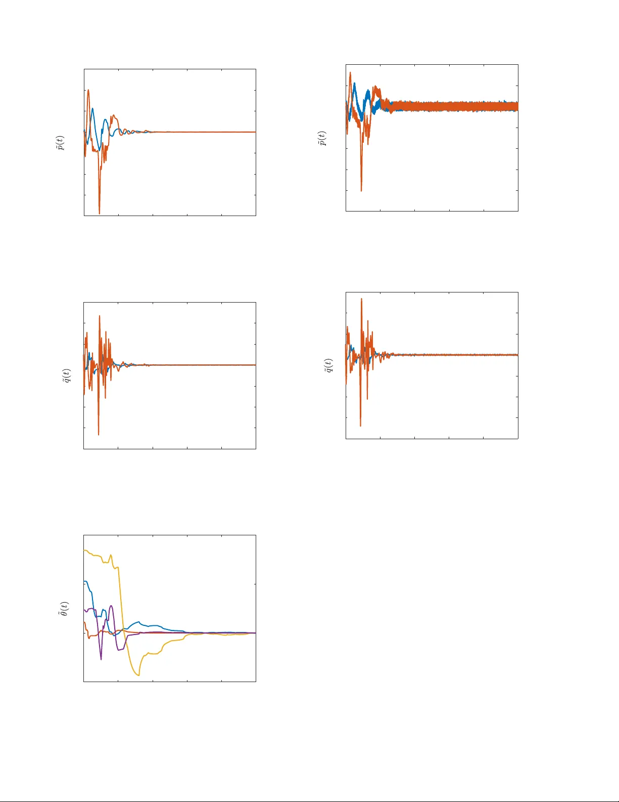
Simultaneous State and Parameter Estimation for Second-Order Nonlinear Systems Rushikesh Kamalapurkar Abstract — In this paper , a concurrent learning based adap- tive observer is developed for a class of second-order nonlinear time-in variant systems with uncertain dynamics. The dev eloped technique results in unif ormly ultimately bounded state and parameter estimation errors. As opposed to persistent excitation which is requir ed for parameter con v ergence in traditional adaptive control methods, the de veloped technique only r equires excitation over a finite time interval to achieve parameter con vergence. Simulation r esults in both noise-free and noisy en vironments ar e presented to validate the design. I . I N T RO D U C T I O N Owing to Increasing reliance on automation and increasing complexity of autonomous systems, the ability to adapt has become an indispensable feature of modern control systems. Traditional adaptive control methods (see, e.g., [1]–[3]) attempt to improve the tracking performance, and in general, do not focus on parameter estimation. While accurate parameter estimation can improv e robustness and transient performance of adapti ve controllers, (see, e.g., [4]– [6]), parameter con ver gence typically requires restrictiv e assumptions such as persistence of excitation. An excitation signal is often added to the controller to ensure persistence of excitation; howe ver , the added signal can cause mechanical fatigue and compromise the tracking performance. Parameter con v ergence can be achie ved under a finite excitation condition using data-driv en methods such as con- current learning (see, e.g., [6]–[8]), where the parameters are estimated by storing data during time-interv als when the system is e xcited, and then utilizing the stored data to driv e adaptation when e xcitation is una v ailable. Concurrent learning has been shown to be an effecti v e tool for adaptive control (see, e.g., [6]–[9]) and adapti ve estimation (see, e.g., [10]–[15]), howe v er , concurrent learning typically requires full state feedback along with accurate numerical estimates of the state-deriv ativ e. Nov el concurrent learning techniques that can be imple- mented using full state measurements but without numerical estimates of the state-deri vati v e are dev eloped in [16] and [17]; howe v er , since full state feedback is typically not av ailable, the development of an output-feedback concurrent learning framework is well-motiv ated. An output feedback concurrent learning technique is developed for second-order linear systems in [18]; howe ver , the implementation critically depends on the certainty equiv alence principle, and hence, is not directly transferable to nonlinear systems. Rushikesh Kamalapurkar is with the School of Mechanical and Aerospace Engineering, Oklahoma State Univ ersity , Stillwater , OK, USA. rushikesh.kamalapurkar@okstate.edu . In this paper, an output feedback concurrent learning method is dev eloped for simultaneous state and parameter estimation in second-order uncertain nonlinear systems. An adaptiv e state-observer is utilized to generate estimates of the state from input-output data. The estimated state trajectories along with the known inputs are then utilized in a novel data- driv en parameter estimation scheme to achieve simultaneous state and parameter estimation. Con v ergence of the state es- timates and the parameter estimates to a small neighborhood of the origin is established under a finite (as opposed to persistent ) excitation condition. The paper is organized as follows. An integral error system that facilitates parameter estimation is dev eloped in Section II. Section III is dedicated to the design of a robust state observer . Section IV details the dev eloped parameter estima- tor . Section V details the algorithm for selection and storage of the data that is used to implement concurrent learning. Section VI is dedicated to a L yapunov-based analysis of the dev eloped technique. Section VII demonstrates the efficac y of the developed method via a numerical simulation and Section VIII concludes the paper . I I . E R RO R S Y S T E M F O R E S T I M A T I O N Consider a second order nonlinear system of the form 1 ˙ p ( t ) = q ( t ) , ˙ q ( t ) = f ( x ( t ) , u ( t )) , y ( t ) = p ( t ) , (1) where p : R ≥ T 0 → R n and q : R ≥ T 0 → R n denote the generalized position states and the generalized velocity states, respectiv ely , x ≜  p T q T  T is the system state, f : R n × R m → R n is locally Lipschitz continuous, and y : R ≥ T 0 → R n denotes the output. The model f is comprised of a known nominal part and an unkno wn part, i.e., f = f o + g , where f o : R n × R m → R n is kno wn and locally Lipschitz and g : R n × R m → R n is unknown and locally Lipschitz. The objective is to design an adaptive estimator to identify the unknown function g , online, using input-output measurements. It is assumed that the system is controlled using a stabilizing input, i.e., x, u ∈ L ∞ . It is further assumed that the signal p , and u are av ailable for feedback. Systems of the form (1) encompass second- order linear systems and Euler-Lagrange models, and hence, represent a wide class of physical plants, including b ut not 1 For a ∈ R , the notation R ≥ a denotes the interval [ a, ∞ ) and the notation R >a denotes the interval ( a, ∞ ) . limited to robotic manipulators and autonomous ground, aerial, and underwater vehicles. Giv en a compact set χ ⊂ R n × R m , and a constant ϵ , the unknown function g can be approximated using basis functions as g ( x, u ) = θ T σ ( x, u ) + ϵ ( x, u ) , where σ : R n × R m → R p and ϵ : R n × R m → R n denote the basis vector and the approximation error , respectiv ely , θ ∈ R p × n is a constant matrix of unkno wn parameters, and there exist σ , θ > 0 such that sup ( x,u ) ∈ χ σ ( x, u ) < σ , sup ( x,u ) ∈ χ ∇ σ ( x, u ) < σ , sup ( x,u ) ∈ χ ϵ ( x, u ) < ϵ , sup ( x,u ) ∈ χ ∇ ϵ ( x, u ) < ϵ , and ∥ θ ∥ < θ . T o obtain an error signal for parameter identification, the system in (1) is expressed in the form ¨ q ( t ) = f o ( x ( t ) , u ( t )) + θ T σ ( x ( t ) , u ( t )) + ϵ ( x ( t ) , u ( t )) . (2) Integrating (2) ov er the interval [ t − τ 1 , t ] for some constant τ 1 ∈ R > 0 and then over the interval [ t − τ 2 , t ] for some constant τ 2 ∈ R > 0 , t ˆ t − τ 2 ( q ( λ ) − q ( λ − τ 1 )) d λ = I f o ( t ) + θ T I σ ( t ) + I ϵ ( t ) , (3) where I denotes the integral operator f 7→ ´ t t − τ 2 ´ λ λ − τ 1 f ( x ( τ ) , u ( τ )) d τ d λ . Using the Fundamental Theorem of Calculus and the fact that q ( t ) = ˙ p ( t ) , the expression in (4) can be rearranged to form the affine system P ( t ) = F ( t ) + θ T G ( t ) + E ( t ) , ∀ t ∈ R ≥ T 0 (4) where P ( t ) ≜      p ( t − τ 2 − τ 1 ) − p ( t − τ 1 ) + p ( t ) − p ( t − τ 2 ) , t ∈ [ T 0 + τ 1 + τ 2 , ∞ ) , 0 t < T 0 + τ 1 + τ 2 . (5) F ( t ) ≜ ( I f o ( t ) , t ∈ [ T 0 + τ 1 + τ 2 , ∞ ) , 0 , t < T 0 + τ 1 + τ 2 , (6) G ( t ) ≜ ( I σ ( t ) , t ∈ [ T 0 + τ 1 + τ 2 , ∞ ) , 0 t < T 0 + τ 1 + τ 2 , (7) and E ( t ) ≜ ( I ϵ ( t ) , t ∈ [ T 0 + τ 1 + τ 2 , ∞ ) , 0 t < T 0 + τ 1 + τ 2 . (8) The affine relationship in (4) is valid for all t ∈ R ≥ T 0 ; howe v er , it provides useful information about the vector θ only after t ≥ T 0 + τ 1 + τ 2 . The knowledge of the generalized velocity , q , is required to compute the matrices F and G . In the follo wing, a rob ust adaptiv e v elocity estimator is de veloped to generate estimates of the generalized velocity . I I I . V E L O C I T Y E S T I M ATO R D E S I G N T o generate estimates of the generalized velocity , a veloc- ity estimator inspired by [19] is de veloped. The estimator is giv en by ˙ ˆ p = ˆ q ˙ ˆ q = f o ( ˆ x, u ) + ˆ θ T σ ( ˆ x, u ) + ν, (9) where ˆ x , ˆ p , ˆ q , and ˆ θ are estimates of x, p, q , and θ , respectiv ely , and ν is a feedback term designed in the following. T o facilitate the design of ν , let ˜ p = p − ˆ p , ˜ q = q − ˆ q , ˜ θ = θ − ˆ θ , and let r ( t ) = ˙ ˜ p ( t ) + α ˜ p ( t ) + η ( t ) , (10) where the signal η is added to compensate for the fact that the generalized velocity state, q , is not measurable. Based on the subsequent stability analysis, the signal η is designed as the output of the dynamic filter ˙ η ( t ) = − β η ( t ) − k r ( t ) − α ˜ q ( t ) , η ( T 0 ) = 0 , (11) where α , k , and β are positi ve constants and the feedback component ν is designed as ν ( t ) = α 2 ˜ p ( t ) − ( k + α + β ) η ( t ) . (12) The design of the signals η and ν to estimate the state from output measurements is inspired by the p − filter [20]. Using the fact that ˜ p ( T 0 ) = 0 , the signal η can be implemented via the integral form η ( t ) = − t ˆ T 0 ( β + k ) η ( τ ) d τ − t ˆ T 0 k α ˜ p ( τ ) d τ − ( k + α ) ˜ p ( t ) . (13) The af fine error system in (4) motiv ates the adaptiv e estimation scheme that follows. The design is inspired by the concurr ent learning technique [21]. Concurrent learning enables parameter conv ergence in adaptiv e control by using stored data to update the parameter estimates. T raditionally , adaptiv e control methods guarantee parameter conv ergence only if the appropriate PE conditions are met [1, Chapter 4]. Concurrent learning uses stored data to soften the PE condition to an excitation condition over a finite time- interval. Concurrent learning methods such as [6] and [8] require numerical differentiation of the system state, and concurrent learning techniques such as [17] and [16] require full state measurements. In the follo wing, a concurrent learning method that utilizes only the output measurements is dev eloped. I V . P A R A M E T E R E S T I M A T O R D E S I G N T o obtain output-feedback concurrent learning update la w for the parameter estimates, a history stack, denoted by H , is utilized. The history stack is a set of ordered pairs n P i , ˆ F i , ˆ G i o M i =1 such that P i = ˆ F i + θ T ˆ G i + E i , ∀ i ∈ { 1 , · · · , M } , (14) where E i is a constant matrix. If a history stack that satisfies (14) is not av ailable a priori, it is recorded online, based on the relationship in (4), by selecting an increasing set of time-instances { t i } M i =1 and letting P i = P ( t i ) , ˆ F i = ˆ F ( t i ) , ˆ G i = ˆ G ( t i ) , (15) where ˆ F ( t ) ≜ ( ˆ I f o ( t ) , t ∈ [ T 0 + τ 1 + τ 2 , ∞ ) , 0 , t < T 0 + τ 1 + τ 2 , (16) ˆ G ( t ) ≜ ( ˆ I σ ( t ) t ∈ [ T 0 + τ 1 + τ 2 , ∞ ) , 0 t < T 0 + τ 1 + τ 2 , (17) where ˆ I denote the operator f 7→ ´ t t − τ 2 ´ λ λ − τ 1 f ( ˆ x ( τ ) , u ( τ )) d τ d λ . In this case, the error term E i is giv en by E i = E ( t i ) + F ( t i ) − ˆ F ( t i ) + θ T  G ( t i ) − ˆ G ( t i )  . Let [ t 1 , t 2 ) be an interval over which the history stack was recorded. Provided the states and the state estimates remain within a compact set χ over I ≜ [ t 1 − τ 1 − τ 2 , t 2 ) , the error terms can be bounded as ∥E i ∥ ≤ L 1 ϵ + L 2 ˜ x I , ∀ i ∈ { 1 , · · · , M } , (18) where ˜ x I ≜ max i ∈{ 1 , ··· ,M } sup t ∈ I ∥ ˜ x ( t ) ∥ and L 1 , L 2 > 0 are constants. The concurrent learning update law to estimate the un- known parameters is designed as ˙ ˆ θ ( t ) = k θ Γ ( t ) M X i =1 ˆ G i  P i − ˆ F i − ˆ θ T ( t ) ˆ G i  T , (19) where k θ ∈ R > 0 is a constant adaptation gain and Γ : R ≥ 0 → R ( 2 n 2 + mn ) × ( 2 n 2 + mn ) is the least-squares gain updated using the update law ˙ Γ ( t ) = β 1 Γ ( t ) − k θ Γ ( t ) G Γ ( t ) . (20) where the matrix G ∈ R p × p is defined as G ≜ P M i =1 ˆ G i ˆ G T i . Using arguments similar to [1, Corollary 4.3.2], it can be shown that pro vided λ min  Γ − 1 ( T 0 )  > 0 , the least squares gain matrix satisfies Γ I p ≤ Γ ( t ) ≤ Γ I p , (21) where Γ and Γ are positi ve constants, and I n denotes an n × n identity matrix. V . P U R G I N G The update law in (19) is moti v ated by the f act that if the full state were av ailable for feedback and if the approxima- tion error , ϵ , were zero, then using  P 1 · · · P n  T =  F 1 · · · F n  T +  G 1 · · · G n  T θ , the param- eters could be estimated via the least squares esti- mate ˆ θ LS = G − 1  G 1 · · · G n   P 1 · · · P n  T − G − 1  G 1 · · · G n   F 1 · · · F n  T . Howe ver , since the history stack contains the estimated terms ˆ F and ˆ G , during the transient period where the state estimation error is large, the history stack does not accurately (within the error bound introduced by ϵ ) represent the system dynamics. Hence, the history stack needs to be purged whene ver better estimates of the state are av ailable. Since the state estimator exponentially drives the estima- tion error to a small neighborhood of the origin, a ne wer estimate of the state can be assumed to be at least as good as an older estimate. A dwell time based greedy purging algorithm is dev eloped in this paper to utilize newer data for estimation while preserving stability of the estimator . The algorithm maintains tw o history stacks, a main his- tory stack and a transient history stack, labeled H and G , respectiv ely . As soon as the transient history stack is full and sufficient dwell time has passed, the main history stack is emptied and the transient history stack is copied into the main history stack. The suf ficient dwell time, denoted by T , is determined using a L yapuno v-based stability analysis. Parameter identification in the developed framework im- poses the following requirement on the history stack H . Definition 1. A history stack n P i , ˆ F i , ˆ G i o M i =1 is called full rank if ther e exists a constant c ∈ R such that 0 < c < λ min { G } , (22) wher e λ min ( · ) denotes the minimum singular value of a matrix. Assumption 1. For a given M ∈ N and c ∈ R > 0 , there exists a set of time instances { t i } M i =1 such that a history stack recorded using (15) is full rank. A singular v alue maximization algorithm is used to select the time instances { t i } M i =1 . That is, a data-point  P j , ˆ F j , ˆ G j  in the history stack is replaced with a new data-point  P ∗ , ˆ F ∗ , ˆ G ∗  , where ˆ F ∗ = ˆ F ( t ) , P ∗ = P ( t ) , and ˆ G ∗ = ˆ G ( t ) , for some t , only if s min   X i  = j ˆ G i ˆ G T i + ˆ G j ˆ G T j   < s min  P i  = j ˆ G i ˆ G T i + ˆ G ∗ ˆ G ∗ T  (1 + ζ ) , (23) where s min ( · ) denotes the minimum singular v alue of a matrix and ζ is a constant. T o simplify the analysis, new data points are assumed to be collected τ 1 + τ 2 seconds after a purging event. Since the history stack is updated using a singular value maximization algorithm, the matrix G is a piece-wise constant function of time. The use of singular value maximization to update the history stack implies that once the matrix G satisfies (22), at some t = T , and for some c , the condition c < λ min ( G ( t )) holds for all t ≥ T . The dev eloped purging method is summarized in Fig. 1. A L yapunov-based analysis of the parameter and the state estimation errors is presented in the following section. V I . S T A B I L I T Y A NA LY S I S Each purging ev ent represents a discontinuous change in the system dynamics; hence, the resulting closed-loop system is a switched system. T o facilitate the analysis of the switched system, let ρ : R ≥ 0 → N denote a switching signal such 1: δ ( T 0 ) ← 0 , η ( T 0 ) ← 0 2: if t > δ ( t ) + τ 1 + τ 2 and a data point is av ailable then 3: if G is not full then 4: add the data point to G 5: else 6: add the data point to G if (23) holds 7: end if 8: if s min ( G ) ≥ ξ η ( t ) then 9: if t − δ ( t ) ≥ T ( t ) then 10: H ← G and G ← 0 ▷ purge and replace H 11: δ ( t ) ← t 12: if η ( t ) < s min ( G ) then 13: η ( t ) ← s min ( G ) 14: end if 15: end if 16: end if 17: end if Fig. 1. Algorithm for history stack pur ging with dwell time. At each time instance t , δ ( t ) stores the last time instance H was purged, η ( t ) stores the highest minimum singular value of G encountered so far , T ( t ) denotes the dwell time, and ξ ∈ (0 , 1] denotes a threshold fraction. that ρ (0) = 1 , and ρ ( t ) = i + 1 , where i denotes the number of times the update H ← G was carried out over the time interval (0 , t ) . For some s ∈ N , let H s denotes the history stack acti ve during the time interval { t | ρ ( t ) = s } ), containing the elements n P si , ˆ F si , ˆ G si o i =1 , ··· ,M , and let E T si be the corresponding error term. T o simplify the notation, let G s ≜ P M i =1 ˆ G si ˆ G T si , and Q s = P M i =1 ˆ G si E T si . Using (14) and (19), the dynamics of the parameter estimation error can be expressed as ˙ ˜ θ ( t ) = − k θ Γ ( t ) G s ( t ) ˜ θ ( t ) − k θ Γ ( t ) Q s ( t ) . (24) Since the functions G s : R ≥ T 0 → R p × p and Q s : R ≥ T 0 → R p × n are piece-wise continuous, the trajectories of (24), and of all the subsequent error systems inv olving G s and and Q s , are defined in the sense of Carathéodory . Algorithm 1 ensures that there exists a constant g > 0 such that λ min { G s } ≥ g , ∀ s ∈ N . Using the dynamics in (1), (9) - (11), and the design of the feedback component in (12), the time-deri vati ve of the error signal r is gi ven by ˙ r ( t ) = − k r ( t )+ ˜ f o ( x, u, ˆ x )+ θ T ˜ σ ( x, u, ˆ x ) − ˜ θ T ˜ σ ( x, u, ˆ x ) + ˜ θ T σ ( x, u ) + ϵ ( x, u ) − α 2 ˜ p + ( k + α ) η , (25) where ˜ σ ( x, u, ˆ x ) = σ ( x, u ) − σ ( ˆ x, u ) and ˜ f o ( x, u, ˆ x ) = f ( x, u ) − f ( ˆ x, u ) . Since ( x, u ) 7→ f ( x, u ) and ( x, u ) 7→ σ ( x, u ) are locally Lipschitz, and since t 7→ u ( t ) is bounded, giv en a compact set ˆ χ ⊂ R n × R m × R n , there exist L f , L σ > 0 such that sup ( x,u, ˆ x ) ∈ ˆ χ    ˜ f o ( x, u, ˆ x )    ≤ L f ∥ ˜ x ∥ and sup ( x,u, ˆ x ) ∈ ˆ χ ∥ ˜ σ ( x, u, ˆ x ) ∥ ≤ L σ ∥ ˜ x ∥ . T o facilitate the analysis, let { T s ∈ R ≥ 0 | s ∈ N } be a set of switching time instances defined as T s = { t | ρ ( τ ) < s + 1 , ∀ τ ∈ [0 , t ) ∧ ρ ( τ ) ≥ s + 1 , ∀ τ ∈ [ t, ∞ ) } . That is, for a giv en switching index s, T s denotes the time instance when the ( s + 1) th subsystem is switched on. The analysis is carried out separately ov er the time intervals [ T s − 1 , T s ) , s ∈ N , where T 1 = T 0 + τ 1 + τ 2 + t M . Since the history stack H is not updated ov er the intervals [ T s − 1 , T s ) , s ∈ N , the matrices G s and Q s are constant o ver each individual interval. The history stack that is active over the interval [ T s , T s +1 ) is denoted by H s . T o ensure boundedness of the trajectories in the interval t ∈ [ T 0 , T 1 ) , the history stack H 1 is arbitrarily selected to be full rank. The analysis is carried out over the aforementioned intervals using the state vectors Z ≜  ˜ p T r T η T vec  ˜ θ  T  T ∈ R 3 n + np and Y ≜  ˜ p T r T η T  T ∈ R 3 n as follows. Interval 1: First, it is established that Z is bounded ov er [ T 0 , T 1 ) , where the bound is O  ∥ Z ( T 0 ) ∥ +    P M i =1 E 1 i    + ϵ  . Given some ε > 0 , the bound on Z is utilized to select gains such that ∥ Y ( T 1 ) ∥ < ε . Interval 2: The history stack H 2 , which is activ e ov er [ T 1 , T 2 ) , is recorded ov er [ T 0 , T 1 ) . W ithout loss of generality , it is assumed that H 2 represents the system better than H 1 (which is arbitrarily selected), that is,    P M i =1 E 1 i    ≥    P M i =1 E 2 i    . The bound on Z over [ T 1 , T 2 ) is then shown to be smaller than that o ver [ T 0 , T 1 ) , which utilized to show that ∥ Y ( t ) ∥ ≤ ε, for all t ∈ [ T 1 , T 2 ) . Interval 3: Using (18), the errors E 3 i are shown to be O ( ∥ Y 3 i ∥ + ϵ ) where Y 3 i denotes the value of Y at the time when the point  P 3 i , ˆ F 3 i , ˆ G 3 i  was recorded. Using the facts that the history stack H 3 , which is active ov er [ T 2 , T 3 ) , is recorded ov er [ T 1 , T 2 ) and ∥ Y ( t ) ∥ ≤ ε, for all t ∈ [ T 1 , T 2 ) , the error    P M i =1 E 3 i    is shown to be O ( ε + ϵ ) . If T 3 = ∞ then it is established that lim sup t →∞ ∥ Z ( t ) ∥ = O ( ε + ϵ ) . If T 3 < ∞ then the fact that the bound on Z ov er [ T 2 , T 3 ) is smaller than that over [ T 1 , T 2 ) is utilized to show that ∥ Y ( t ) ∥ ≤ ε, for all t ∈ [ T 2 , T 3 ) . The analysis is then continued in an inductive argument to show that lim sup t →∞ ∥ Z ( t ) ∥ = O ( ε + ϵ ) and ∥ Y ( t ) ∥ ≤ ε, for all t ∈ [ T 2 , ∞ ) . The stability result is summarized in the follo wing theo- rem. Theorem 1. Let ε > 0 be giv en. Let the history stacks H and G be populated using the algorithm detailed in Fig. 1. Let the learning gains be selected to satisfy the sufficient gain conditions in (28), (29), (34), and (38). Let T ∈ R > 0 be a time instance such that the system states are exciting over [ T 0 , T ] , that is, the history stack can be replenished if purged at an y time t ∈ [ T 0 , T ] . Assume that ov er each switching interval { t | ρ ( t ) = s } , the dwell-time, T , is selected such that T ( t ) = T s , where T s is selected to be large enough to satisfy (37). Furthermore assume that the excitation interv al is lar ge enough so that T 2 < T . 2 Then, lim sup t →∞ ∥ Z ( t ) ∥ = O ( ε + ϵ ) . Pr oof. Provided H 1 is full rank, then the candidate L yapuno v function 2 V ( Z , t ) ≜ α 2 ˜ p T ˜ p + r T r + η T η + tr  ˜ θ T Γ − 1 ( t ) ˜ θ  (26) can be utilized to establish boundedness of trajectories over [ T s − 1 , T s ) . The candidate L yapunov function satisfies v ∥ Z ∥ 2 ≤ V ( Z, t ) ≤ v ∥ Z ∥ 2 , (27) where v ≜ 1 2 max  1 , α 2 , 1 / Γ  and v ≜ 1 2 min  1 , α 2 , 1 / Γ  . The time-deriv ativ e of V along the trajectories of (10), (11), (20), (24), and (25) is giv en by ˙ V = − α 3 ˜ p T ˜ p − k r T r − β η T η − 1 2 tr  ˜ θ T  k θ G 1 + β 1 Γ − 1  ˜ θ  + r T ˜ f o + r T θ T ˜ σ + r T ˜ θ T ˆ σ + r T ϵ − k θ tr  ˜ θ T Q s  . Using the Cauchy-Schwartz inequality , the deriv ativ e can be bounded as ˙ V ≤ − α 3 ∥ ˜ p ∥ 2 − k ∥ r ∥ 2 − β ∥ η ∥ 2 − 1 2 a    ˜ θ    2 + L f ∥ r ∥ ∥ ˜ x ∥ + ∥ r ∥ θ L σ ∥ ˜ x ∥ + ∥ r ∥    ˜ θ    ∥ ˆ σ ∥ + ∥ r ∥ ϵ + k θ    ˜ θ    Q s , where a = k θ g + β 1 Γ , and Q s is a positi ve constant such that Q s ≥ ∥ Q s ∥ . Provided k > max  2 (4 + α )  L f + θ L σ  , 12 σ 2 a  , α 3 > (1 + α )  L f + θ L σ  , β >  L f + θ L σ  , (28) Y oung’ s inequality and nonlinear damping can be used to conclude that ˙ V ≤ − α 3 2 ∥ ˜ p ∥ 2 − k 4 ∥ r ∥ 2 − β 2 ∥ η ∥ 2 − a 6    ˜ θ    2 −  k 8 − 3 L σ 2 a ∥ ˜ x ∥ 2  ∥ r ∥ 2 + ϵ 2 k + 3 k 2 θ 2 a Q 2 s , Since ∥ ˜ x ∥ 2 ≤ (1 + α ) ∥ Z ∥ 2 , ˙ V ≤ − ν  ∥ Z ∥ − ι s ν  , in the domain D ≜ ( Z ∈ R 3 n + np | ∥ Z ∥ < s k a 12 L σ (1 + α ) ) . That is, ˙ V is negati ve definite on D pro vided ∥ Z ∥ > p ι s ν > 0 , where v ≜ 1 2 min  α 3 , k / 2 , β , a / 3  and ι s ≜ ϵ 2 k + 3 k 2 θ 2 a Q 2 s . Theorem 4.18 from [22] can then be inv oked to conclude that provided k > 15 L σ (1 + α ) av max  V s , v ι 1 v  , (29) where V s ≥ ∥ V ( Z ( T s − 1 ) , T s − 1 ) ∥ is a constant, then ˙ V ≤ − v v V + ι s , ∀ t ∈ [ T s − 1 , T s ) . 2 A minimum of two purges are required to remove the randomly initialized data, and the data recorded during transient phase of the deri vati ve estimator from the history stack. In particular , ∀ t ∈ [ T 0 , T 1 ) , V ( Z ( t ) , t ) ≤  V 1 − v v ι 1  e − v v ( t − T 0 ) + v v ι 1 , (30) where V 1 > 0 is a constant such that | V ( Z ( T 0 ) , T 0 ) | ≤ V 1 . Hence, ∀ t ∈ [ T 0 , T 1 ) ,    ˜ θ ( t )    ≤ θ 1 ≜ r 1 v max ( q V 1 , r v v ι 1 ) . (31) If it were possible to use the inequality in (30) to conclude that over [ T 0 , T 1 ) , V ( Z ( t ) , t ) ≤ V ( Z ( T 0 ) , T 0 ) , then an inductiv e ar gument could be used to sho w that the trajectories decay to a neighborhood of the origin. Howe ver , unless the history stack can be selected to hav e arbitrarily large minimum singular value (which is generally not possible), the constant v v ι 1 cannot be made arbitrarily small using the learning gains. Since ι s depends on Q s , it can be made smaller by reducing the estimation errors and thereby reducing the errors associated with the data stored in the history stack. T o that end, consider the candidate L yapuno v function W ( Y ) ≜ α 2 2 ˜ p T ˜ p + 1 2 r T r + 1 2 η T η . (32) The candidate L yapunov function satisfies w ∥ Y ∥ 2 ≤ W ( Y , t ) ≤ w ∥ Y ∥ 2 , (33) where w ≜ 1 2 max  1 , α 2  , w ≜ 1 2 min  1 , α 2  . In the interval [ T s − 1 , T s ) , the time-deriv ativ e of W is given by ˙ W = − α 3 ˜ p T ˜ p − k r T r − β η T η + r T  ˜ f o +  θ T − ˜ θ T  ˜ σ  + r T  ˜ θ T σ + ϵ  Using the Cauchy-Schwartz inequality , the deriv ativ e ˙ W can be bounded as ˙ W = − α 3 ∥ ˜ p ∥ 2 − k ∥ r ∥ 2 − β ∥ η ∥ 2 +  L f +  θ + θ s  L σ  ∥ r ∥ ∥ ˜ x ∥ + ( θ s σ + ϵ ) ∥ r ∥ , where θ s > 0 is a constant such that θ s ≥ sup t ∈ [ T s − 1 ,T s )    ˜ θ ( t )    . Consider the time interv al [ T 0 , T 1 ) . Provided k ≥ 1 + θ 2 1 +  L f +  θ + θ 1  L σ  (4 + α ) α 3 ≥ (1 + α )  L f +  θ + θ 1  L σ  β ≥  L f +  θ + θ 1  L σ  (34) then ˙ W ≤ − w w W + λ, where w = 1 2 min  α 3 , k , β  and λ = σ 2 + ϵ 2 2 . That is, for all t ∈ [ T 0 , T 1 ) , W ( Y ( t ) , t ) ≤  W 1 − w w λ  e − w w ( t − T 0 ) + w w λ, (35) where W 1 > 0 is a constant such that | W ( Y ( T 0 )) | ≤ W 1 . In particular , ∀ t ∈ [ T 0 , T 1 ) . ∥ Y ( t ) ∥ ≤ s 1 w max  W 1 , w w λ  ≜ ∥ Y ∥ 1 . (36) Provided the dwell time T s is large enough so that  W s − w w λ  e − w w T s ≤ w w λ,  V s − v v ι s  e − v v T s ≤ v v ι s , (37) then from (30) and (35), W ( Y ( T 1 )) ≤ 2 wλ w and V ( Z ( T 1 ) , T 1 ) ≤ 2 v ι 1 v . In particular , ∥ Y ( T 1 ) ∥ ≤ q 2 wλ ww and ∥ Z ( T 1 ) ∥ ≤ q 2 v ι 1 v v . Note that the bound on Y ( T 1 ) can be made arbitrarily small by increasing k , α, and β . Now the interv al [ T 1 , T 2 ) is considered. Since the history stack H 2 which is acti ve during [ T 1 , T 2 ) is recorded during [ T 0 , T 1 ) , the bound in (18) can be used to sho w that Q 2 = O  ∥ Y ∥ 1 + ϵ  . Since H 1 is independent of the system trajectories, Q 1 can be selected such that Q 2 < Q 1 , and hence, ι 2 < ι 1 . Thus, pro vided the constant V 1 (and as a result, the gain k ) is selected large enough so that 2 v ι 1 v < V 1 , (38) the gain condition in (29) holds over [ T 1 , T 2 ) , and hence, a similar L yapunov-based analysis, along with the bound V 2 = 2 v ι 1 v can be utilized to conclude that ∀ t ∈ [ T 1 , T 2 ) ,    ˜ θ ( t )    ≤ r v v v max  √ 2 ι 1 , √ ι 2  ≜ θ 2 . (39) The sufficient condition in (38) implies that V 2 < V 1 and hence, (31) and ι 2 < ι 1 imply that θ 2 < θ 1 . Since θ 2 < θ 1 , the gain conditions in (34) hold o ver the interv al [ T 1 , T 2 ) . A L yapuno v-based analysis similar to (32)-(36) yields ∥ Y ( t ) ∥ ≤ q 1 w max  W 2 , w w λ  . From (37), W 2 = 2 wλ w , and hence, ∀ t ∈ [ T 1 , T 2 ) , ∥ Y ( t ) ∥ ≤ s 2 w λ w w ≜ ∥ Y ∥ 2 . (40) Now , the interv al [ T 2 , T 3 ) is considered. Since the history stack H 3 which is acti ve during [ T 2 , T 3 ) is recorded during [ T 1 , T 2 ) , the bounds in (18) and (40) can be used to show that Q 3 = O  ∥ Y ∥ 2 + ϵ  . By selecting W 1 large enough, it can be ensured that ∥ Y ∥ 2 < ∥ Y ∥ 1 , and hence, Q 3 < Q 2 , which implies ι 3 < ι 2 . Provided T 2 satisfies (37), then  V 2 − v v ι 2  e − v v ( T 2 − T 1 ) ≤ v v ι 2 , which implies V 3 = v v ι 2 , and hence, V 3 < V 2 and θ 3 < θ 2 . Therefore, the gain conditions in (28), (29), and (34) are satisfied ov er [ T 2 , T 3 ) . Since the gain conditions are satisfied, a L yapunov-based analysis similar to (32)-(36) yields ∥ Y ( t ) ∥ ≤ q 2 wλ ww , ∀ t ∈ [ T 2 , T 3 ) . Given any ε > 0 , the gains α, β , and k can be selected large enough to satisfy ∥ Y ∥ 2 ≤ ε, and hence, ∥ Y ( t ) ∥ ≤ ε, ∀ t ∈ [ T 2 , T 3 ) . Furthermore, a similar L yapunov-based analysis as (26) - (30) yields V ( Z ( t ) , t ) ≤  V 3 − v v ι 3  e − v v ( t − T 2 ) + v v ι 3 , ∀ t ∈ [ T 2 , T 3 ) . If T 3 = ∞ then lim sup t →∞ V ( Z ( t ) , t ) ≤ v v ι 3 , which, from T ABLE I S I MU L A T I ON PAR A M ET E R S F O R T H E D I FFE R E NT S I MU L A T I ON RU N S . T H E PA R AM E T E RS A RE S E LE C T ED U S IN G T R I A L A N D E R RO R . Noise V ariance Parameter 0 0.001 T 1 0.5 0.9 T 2 0.3 0.5 N 50 150 Γ ( t 0 ) I 4 I 4 β 1 0.5 0.5 α 2 2 k 10 10 β 2 2 ζ 0 0 ξ 0.95 0.95 k θ 0.5 / N 0.5 / N 0 10 20 30 40 50 Time (s) -2 0 2 4 6 8 10 Fig. 2. T rajectories of the parameter estimation errors using noise-free position measurements. Q 3 = O  ∥ Y ∥ 2 + ϵ  and ι 3 = ϵ 2 k + 3 k 2 θ 2 a Q 2 3 implies that lim sup t →∞ ∥ Z ( t ) ∥ = O ( ε + ϵ ) . If T 3  = ∞ then an inductiv e continuation of the L yapuno v-based analysis to the time intervals [ T s − 1 , T s ) shows that provided the dwell time T s satisfies (37), the gain conditions in (28), (29), and (34) are satisfied for all t > T 3 , the state Y satisfies ∥ Y ( t ) ∥ ≤ ε, ∀ t > T 1 , (41) and Q s ≤ Q s − 1 , ι s ≤ ι s − 1 , V s ≤ V s − 1 , and θ s ≤ θ s − 1 , for all s > 3 . The bound in (41) and the fact that Q s = O  ∥ Y ∥ s − 1 + ϵ  indicate that Q s = O ( ε + ϵ ) , ∀ s ∈ N . Furthermore, V ( Z ( t ) , t ) ≤  V s − v v ι s  e − v v ( t − T s − 1 ) + v v ι s , ∀ t ∈ [ T s − 1 , T s ) , ∀ s ∈ N , which, along with the dwell time requirement, implies that lim sup t →∞ V ( Z ( t ) , t ) ≤ v v ι s , and hence, lim sup t →∞ ∥ Z ( t ) ∥ = O ( ε + ϵ ) . V I I . S I M U L A T I O N The de veloped technique is simulated using a model for a two-link robot manipulator arm. The uncertainty g ( x, u ) is linearly parameterizable as g T ( x, u ) = θ T σ ( x, u ) . That 0 10 20 30 40 50 Time (s) -2 -1.5 -1 -0.5 0 0.5 1 1.5 Fig. 3. Trajectories of the generalized position estimation errors using noise-free position measurements. 0 10 20 30 40 50 Time (s) -8 -6 -4 -2 0 2 4 6 Fig. 4. Trajectories of the generalized velocity estimation errors using noise-free position measurements. 0 10 20 30 40 50 Time (s) -5 0 5 10 Fig. 5. T rajectories of the parameter estimation errors with a Gaussian measurement noise (variance = 0.001). 0 10 20 30 40 50 Time (s) -2.5 -2 -1.5 -1 -0.5 0 0.5 1 Fig. 6. T rajectories of the generalized position estimation errors with a Gaussian measurement noise (variance = 0.001). 0 10 20 30 40 50 Time (s) -8 -6 -4 -2 0 2 4 6 Fig. 7. T rajectories of the generalized v elocity estimation errors with a Gaussian measurement noise (variance = 0.001). is, the selected model belongs to a sub-class of systems defined by (1), where the function approximation error , ε , is zero. Since the ideal parameters, θ , are uniquely known, the selected model facilitates quantitati ve analysis of the parameter estimation error . The dynamics of the arm are described by (1), where f 0 ( x, u ) = − ( M ( p )) − 1 V m ( p, q ) q + ( M ( p )) − 1 u, g T ( x, u ) = θ T  ( M ( p )) − 1 ( M ( p )) − 1  D ( q )  T . (42) In (42), u ∈ R 2 is the control input, D ( q ) ≜ diag [tanh ( q 1 ) , tanh ( q 2 )] , M ( p ) ≜  p 1 + 2 a 3 c 2 ( p ) , a 2 + a 3 c 2 ( p ) a 2 + a 3 c 2 ( p ) , a 2  , and V m ( p, q ) ≜  − a 3 s 2 ( p ) q 2 , − a 3 s 2 ( p ) ( q 1 + q 2 ) a 3 s 2 ( p ) q 1 , 0  , where c 2 ( p ) = cos ( p 2 ) , s 2 ( p ) = sin ( p 2 ) , and a 1 = 3 . 473 , a 2 = 0 . 196 , and a 3 = 0 . 242 are constants. The system has four unknown parameters. The ideal values of the unknown parameters are θ =  5 . 3 1 . 1 8 . 45 2 . 35  T . The contribution of this paper is the design of a parameter estimator and a v elocity observer . The controller is assumed to be any controller that results in bounded system response. In this simulation study , the controller, u , is designed so that the system tracks the trajectory p 1 ( t ) = p 2 ( t ) = sin (3 t ) + sin (2 t ) . The simulation is performed using Euler forward nu- merical integration using a sample time of T s = 0 . 0005 seconds. Past τ 1 + τ 2 T s values of the generalized position, p , and the control input, u , are stored in a b uffer . The matrices P , ˆ G , and ˆ F for the parameter update law in (19) are computed using trapezoidal integration of the data stored in the aforementioned buf fer . V alues of P , ˆ G , and ˆ F are stored in the history stack and are updated according to the algorithm detailed in Fig. 1. The initial estimates of the unknown parameters are se- lected to be zero, and the history stack is initialized so that all the elements of the history stack are zero. Data is added to the history stack using a singular v alue maximization algorithm. T o demonstrate the utility of the dev eloped method, three simulation runs are performed. In the first run, the observer is assumed to ha ve access to noise free measurements of the generalized position. In the second run, a zero-mean Gaus- sian noise with v ariance 0.001 is added to the generalized position signal to simulate measurement noise. The values of various simulation parameters selected for the three runs are provided in T able I. Figure 2 demonstrates that in absence of noise, the dev eloped parameter estimator dri ves the state estimation error , ˜ x , and the parameter estimation error , ˜ θ , close to the origin. Figures 5 - 7 indicate that the developed technique can be utilized in the presence of measurement noise, with expected degradation of performance. V I I I . C O N C L U S I O N This paper dev elops a concurrent learning based adaptiv e observer and parameter estimator to simultaneously estimate the unknown parameters and the generalized velocity of second-order nonlinear systems using generalized position measurements. The developed technique utilizes a dynamic velocity observer to generate state estimates necessary for data-driv en adaptation. A purging algorithm is dev eloped to improv e the quality of the stored data as the state estimates con ver ge to the true state. By integrating n − times, the dev eloped method can be generalized to higher-order linear systems. Simulation results indicate that the de veloped method is robust to measurement noise. A theoretical analysis of the dev eloped method under measurement noise and process noise is a subject for future research. Future efforts will also focus on the examination the ef fect of the integration intervals, τ 1 and τ 2 , on the performance of the developed estimator . R E F E R E N C E S [1] P . Ioannou and J. Sun, Robust Adaptive Contr ol . Prentice Hall, 1996. [2] S. Sastry and M. Bodson, Adaptive Contr ol: Stability , Conver gence , and Robustness . Upper Saddle River , NJ: Prentice-Hall, 1989. [3] M. Krstic, I. Kanellakopoulos, and P . V . K okotovic, Nonlinear and Adaptive Control Design . New Y ork, NY , USA: John Wile y & Sons, 1995. [4] M. A. Duarte and K. Narendra, “Combined direct and indirect ap- proach to adaptive control, ” IEEE T r ans. A utom. Contr ol , vol. 34, no. 10, pp. 1071–1075, Oct 1989. [5] M. Krsti ´ c, P . V . Kokoto vi ´ c, and I. Kanellakopoulos, “T ransient- performance improvement with a new class of adaptive controllers, ” Syst. Control Lett. , vol. 21, no. 6, pp. 451–461, 1993. [6] G. Chowdhary and E. Johnson, “ A singular value maximizing data recording algorithm for concurrent learning, ” in Pr oc. Am. Control Conf. , 2011, pp. 3547–3552. [7] G. Chowdhary , T . Y ucelen, M. Mühle gg, and E. N. Johnson, “Con- current learning adaptiv e control of linear systems with exponentially con vergent bounds, ” Int. J. Adapt. Contr ol Signal Pr ocess. , vol. 27, no. 4, pp. 280–301, 2013. [8] S. Kersting and M. Buss, “Concurrent learning adaptive identification of piecewise affine systems, ” in Proc. IEEE Conf. Decis. Control , Dec. 2014, pp. 3930–3935. [9] G. Cho wdhary , M. Mühlegg, J. How , and F . Holzapfel, “Concurrent learning adaptive model predictive control, ” in Advances in Aer ospace Guidance, Navigation and Contr ol , Q. Chu, B. Mulder, D. Choukroun, E.-J. v an Kampen, C. de V isser , and G. Looye, Eds. Springer Berlin Heidelberg, 2013, pp. 29–47. [10] H. Modares, F . L. Lewis, and M.-B. Naghibi-Sistani, “Integral rein- forcement learning and experience replay for adaptive optimal control of partially-unknown constrained-input continuous-time systems, ” Au- tomatica , vol. 50, no. 1, pp. 193–202, 2014. [11] R. Kamalapurkar , J. Klotz, and W . E. Dixon, “Concurrent learning- based online approximate feedback Nash equilibrium solution of N -player nonzero-sum differential games, ” IEEE/CAA J. Autom. Sin. , vol. 1, no. 3, pp. 239–247, Jul. 2014, Special Issue on Extensions of Reinforcement Learning and Adaptive Control. [12] B. Luo, H.-N. W u, T . Huang, and D. Liu, “Data-based approximate policy iteration for affine nonlinear continuous-time optimal control design, ” Automatica , 2014. [13] R. Kamalapurkar, P . W alters, and W . E. Dixon, “Model- based reinforcement learning for approximate optimal regulation, ” Automatica , vol. 64, pp. 94–104, Feb. 2016. [14] T . Bian and Z.-P . Jiang, “V alue iteration and adaptiv e dynamic programming for data-dri ven adaptiv e optimal control design, ” Au- tomatica , vol. 71, pp. 348–360, 2016. [15] R. Kamalapurkar, J. A. Rosenfeld, and W . E. Dixon, “Efficient model-based reinforcement learning for approximate online optimal control, ” Automatica , vol. 74, pp. 247–258, Dec. 2016. [16] R. Kamalapurkar , B. Reish, G. Chowdhary , and W . E. Dixon, “Concurrent learning for parameter estimation using dynamic state-deriv ativ e estimators, ” IEEE T rans. A utom. Control , 2017, to appear . [17] A. Parikh, R. Kamalapurkar , and W . E. Dixon, “Integral concurrent learning: Adapti ve control with parameter conv ergence without PE or state deriv atives, ” 2017, submitted, see arXiv:1512.03464, automatica. [18] R. Kamalapurkar , “Online output-feedback parameter and state esti- mation for second order linear systems, ” in Pr oc. Am. Contr ol Conf. , 2017, to appear , see also, [19] H. T . Dinh, R. Kamalapurkar, S. Bhasin, and W . E. Dixon, “Dynamic neural network-based robust observers for uncertain nonlinear systems, ” Neural Netw . , vol. 60, pp. 44–52, Dec. 2014. [20] B. Xian, M. S. de Queiroz, D. M. Dawson, and M. McIntyre, “ A discontinuous output feedback controller and v elocity observer for nonlinear mechanical systems, ” Automatica , vol. 40, no. 4, pp. 695– 700, 2004. [21] G. Chowdhary , “Concurrent learning for conv ergence in adaptive control without persistency of excitation, ” Ph.D. dissertation, Georgia Institute of T echnology , Dec. 2010. [22] H. K. Khalil, Nonlinear Systems , 3rd ed. Upper Saddle Riv er , NJ: Prentice Hall, 2002.