Continuous-time Discounted Mirror-Descent Dynamics in Monotone Concave Games

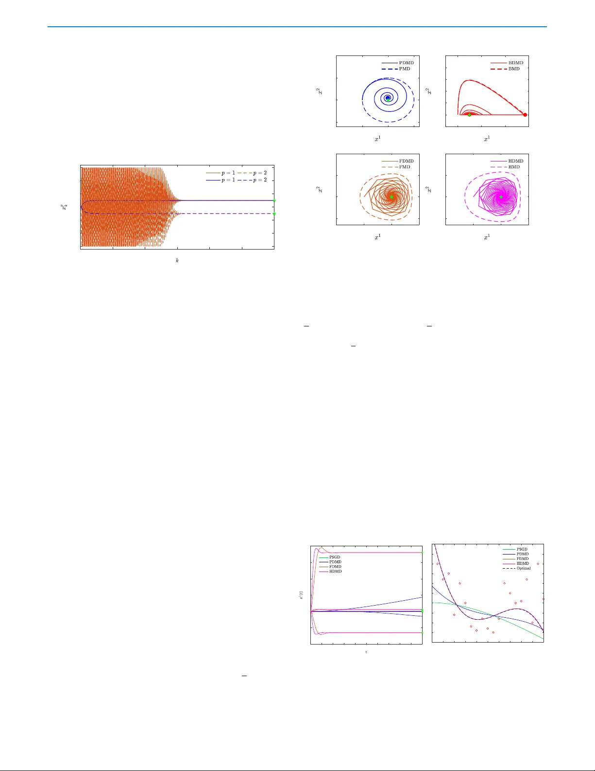
1 Continuous-time Discounted Mirror-Descent Dynamics in Monotone Conca v e Games Bolin Gao and Lacra P a v el Abstract — W e consider concave contin uous-kernel games char - acterized by monotonicity properties and propose discounted mir- ror descent-type dynamics. We introduce two classes of dynam- ics whereby the associated mirror map is constructed based on a strongl y con vex or a Legendre regularizer . Depending on the properties of the regularizer , we show that these new dynamics can converge asymptotically in concave games with monotone (negative) pseudo-gradient. Furthermore, we show that when the regularizer enjoys str ong con vexity , the resulting d ynamics can con verge even in games with hypo-monotone (negative) pseudo- gradient, which corresponds to a shortage of monotonicity . I . I N T R O D U C T I O N One of the earliest works on solving continuous-kernel concave games is the work of Rosen [29]. The continuous-time gradient type dynamics was sho wn to conv erge to the Nash equilibrium in games that satisfy a so-called diagonally strictly conca ve condition, roughly equiv alent to the pseudo-gradient being a strictly monotone operator . Recently , research on solving monotone games has seen a surge. Both continuous-time dynamics and discrete-time algorithms hav e been de- veloped, mostly for games with strictly (strongly) monotone pseudo- gradient. For (non-strictly) monotone only games, no continuous- time dynamics exist. Discrete-time algorithms hav e been proposed, based on either proximal regularization, [28], inexact proximal best- response, [17] or T ikhonov type regularization, [19], and recently extended to generalized Nash equilibrium, e.g. [20], [21]. All these works are done in a discr ete-time setting and the dynamics ev olve in the primal space of decision v ariables (and possibly multipliers). W ith the exception of [19], these algorithms are applicable only in games with “cheap” (inexpensiv e) proximal/resolvent ev aluation, [28]. In this note we propose a family of continuous-time discounted mirr or descent dynamics, whereby the dynamics e v olves in the space of dual (pseudo-gradient) variables. The mapping from the dual back to the primal space of decision v ariables is done via a mirror map, constructed based on two general classes of regularizers. Depending on the properties of the regularizer , we sho w that these dynamics can con v erge asymptotically in merely monotone, and ev en hypo- monotone, conca ve games. T o the best of our knowledge, these are the first such dynamics in the literature. Our novel contributions consist in relating the con ver gence of the dynamics to the properties of the con ve x conjugate of the regularizer . Literatur e r e view: Mirror descent algorithms hav e found numerous applications in recent years, e.g. in distrib uted optimization [2], online learning [4], and v ariational inequality problems [5]. They fall into the class of so-called primal-dual algorithms; the name mirr or descent refers to the two iterative steps: a mapping of the primal variable into a dual space (in the sense of con ve x conjugate), followed by a mapping of the dual variable, or some post-processing of it, back into the primal space via a mirror map. The mirror descent algorithm (MD A) introduced by Nemrovskii and Y udin [1], was originally proposed as a generalization of projected gradient descent (PGD) for constrained optimization. The authors of [31] have shown that MDA B. Gao and L. Pa vel are with the Depar tment of Electr ical and Computer Engineering, University of T oronto , T oronto, ON, M5S 3G4, Canada. Emails: bolin.gao@mail.utoronto.ca, pavel@control.utoronto.ca possesses better rate of con ver gence as compared to the PGD, which makes it especially suitable for large-scale optimization problems. Other types of algorithms can be seen as equiv alent to or special cases of MD A, e.g. dual av eraging [3] and follow-the-leader [4]. A continuous-time v ersion of MD A, referred to as the mirror descent (MD) dynamics, [12], [15], captures many existing continuous-time dynamics as special cases, such as the gradient flo w [12], [15], saddle- point dynamics [9] and pseudo-gradient dynamics [10]. In the context of multi-agent games, mirror descent-like algorithms hav e been applied to continuous-kernel games [13], finite-games [6], [7], and population games. The primal space is taken to be the space of decisions/strategies, and the dual space is the space of payoff vectors (in finite games) or pseudo-gradient vectors (in continuous-kernel games). Zhou et al. [13] introduced the concept of variationally stable concav e game and showed that, under variational stability , the iterates of an online MDA conv erge to the set of Nash equilibria, whenever the step-size is slowly vanishing step- size sequence and that the mirror map satisfies a F enchel coupling conforming condition [13]. Since all concave games with strictly monotone pseudo-gradient are variationally stable concav e games, therefore the algorithm conv erges in all strictly monotone games. Howe v er , there are games with a (unique) Nash equilibrium that is not necessarily variationally stable, e.g. zero-sum (monotone) games. While finding the Nash equilibrium of strictly monotone games is an important problem, con v ergence in such games does not necessarily imply con vergence in monotone (but not strictly monotone) games. Contributions: Motiv ated by the above, in this work we propose two classes of continuos-time discounted MD dynamics for concave, continuous-kernel games. The discounting is performed on the dual step of the mirror descent, which generates a weighted-aggr e gation effect similar to the dynamics studied for finite-action games in [7]. Discounting is known to foster conv ergence and eliminate cycling in games, as sho wn in monotone games or zero-sum games [7], [24]. By exploiting properties of the mirror map in the two classes as well as the discounting effect, we show that these dynamics con ver ge asymptotically to the perturbed equilibria of concav e games with monotone (not necessarily strictly monotone) pseudo-gradient. Under certain conditions, they can e ven con ver ge in concave games with hypo-monotone pseudo-gradient. T o the best of our knowledge, these are the first such results. Our con ver gence analysis uses a L yapunov function giv en by a Bregman div ergence. W e note that recently [32] identified the Bre gman diver gence as a natural L yapunov candidate for a variety of systems, elegantly tying with existing results on mirror descent dynamics [12]. While the dynamics are in the dual space as in [7], herein we consider continuous-kernel games rather than finite-action games. Furthermore, compared to [7] we set up a general framew ork in terms of two classes of regularizers, matched to the geometry of the action set. For either strongly conv ex or Leg- endre regularizers, we provide conv ergence guarantees in monotone (hypo-monotone) games and present several example discounted MD dynamics. In fact, one such example recovers the dynamics in [7] if the action set is specialized to a simplex geometry and the regularizer taken as a particular entropy e xample. Another example dynamics can be seen as the continuous-time dual counterpart to the discrete-time T ikhonov (primal) regularization, [19]. Compared to the undiscounted 2 MD [13], our discounted MD dynamics can conv erge in (not strictly) monotone games, and even in hypo-monotone games. A short version will appear in [39], with two example dynamics. Here we propose two general classes, present proofs (omitted from [39]), additional example dynamics and numerical results. The paper is organized as follo ws. In Section II, we provide preliminary background. Section III presents the problem setup and introduces a general form of the discounted mirror descent (DMD) dynamics. In Section IV , we construct two classes of DMD and prove their conv ergence. In Section V , we construct sev eral examples of DMD from each class. W e present numerical results in Section VI and conclusions in Section VII. I I . B A C K G R O U N D A. Conve x Sets, Fenchel Duality and Monotone Operators The follo wing is from [23], [25], [28]. Giv en a con v ex set C ⊆ R n , the (relative) interior of the set is denoted as ( rin t( C ) ) int( C ) . rin t( C ) coincides with in t( C ) whene ver int( C ) is non-empty . The closure of C is denoted as cl( C ) , and the relative boundary of C is defined as rb d( C ) = cl( C ) \ rin t( C ) . The indicator function over C is denoted by δ C . The normal cone of C is defined as N Ω ( x ) = { v ∈ R n | v > ( y − x ) ≤ 0 , ∀ y ∈ C } and π C ( x ) = argmin y ∈C k y − x k 2 2 is the Euclidean projection of x onto C . Let E = R n be endowed with norm k · k and inner product h· , ·i . An extended real-valued function is a function f that maps from E to [ −∞ , ∞ ] . The (ef fectiv e) domain of f is dom( f ) = { x ∈ E : f ( x ) < ∞} . A function f : E → [ −∞ , ∞ ] is proper if it does not attain the value −∞ and there e xists at least one x ∈ E such that f ( x ) < ∞ ; it is closed if its epigraph is closed. A function f : E → [ −∞ , ∞ ] is supercoerciv e if lim k x k→∞ f ( x ) / k x k → ∞ . Let ∂ f ( x ) denote a subgradient of f at x and ∇ f ( x ) the gradient of f at x , if f is differentiable. Suppose f is a closed con v ex proper on E with in t(dom( f )) 6 = ∅ , then f is essentially smooth if f is differentiable on in t(dom( f )) and lim k → ∞ k∇ f ( x k ) k → ∞ whene ver { x k } ∞ k =1 is a sequence in int(dom( f )) conv erging towards a boundary point. f is essentially strictly con vex if f is strictly con ve x on every con vex subset of dom( ∂ f ) . A function f is Legendre if it is both essentially smooth and essentially strictly conv ex. Giv en f , the function f ? : E ? → [ −∞ , ∞ ] defined by f ? ( z ) = sup x ∈ E  x > z − f ( x )  , is called the conjugate function of f , where E ? is the dual space of E , endowed with the dual norm k · k ? . f ? is closed and con v ex if f is proper . By Fenchel’ s inequality , for any x ∈ E , z ∈ E ? , f ( x )+ f ? ( z ) ≥ z > x (with equality if and only if z ∈ ∂ f ( x ) for proper and con v ex f , or x ∈ ∂ f ? ( z ) if in addition f is closed [23, Theorem 4.20]). The Bregman div ergence of a proper, closed, con vex function f , differentiable ov er dom( ∂ f ) , is D f : dom( f ) × dom( ∂ f ) → R , D f ( x, y ) = f ( x ) − f ( y ) − ∇ f ( y ) > ( x − y ) . F : C ⊆ R n → R n is monotone if ( F ( z ) − F ( z 0 )) > ( z − z 0 ) ≥ 0 , ∀ z , z 0 ∈ C . F is L -Lipschitz if k F ( z ) − F ( z 0 ) k ≤ L k z − z 0 k , for some L > 0 and is β -cocoer cive if ( F ( z ) − F ( z 0 ) > ( z − z 0 ) ≥ β k F ( z ) − F ( z ) 0 k 2 , ∀ z , z 0 ∈ C for some β > 0 . B. N -Play er Concav e Games Let G = ( N , { Ω p } p ∈N , {U p } p ∈N ) be a game, where N = { 1 , . . . , N } is the set of players, Ω p ⊆ R n p is the set of player p ’ s strategies (actions). W e denote the strategy (action) set of player p ’ s opponents as Ω − p ⊆ Q q ∈N ,q 6 = p R n q . W e denote the set of all the players strategies as Ω = Q p ∈N Ω p ⊆ Q p ∈N R n p = R n , n = P p ∈N n p . W e refer to U p : Ω → R , x 7→ U p ( x ) as player p ’ s real-valued payoff function, where x = ( x p ) p ∈N ∈ Ω is the action profile of all players, and x p ∈ Ω p is the action of player p . W e also denote x as x = ( x p ; x − p ) where x − p ∈ Ω − p is the action profile of all players except p . Assumption 1. For all p ∈ N , i. Ω p is a non-empty , closed, con vex, subset of R n p , ii. U p ( x p ; x − p ) is (jointly) continuous in x = ( x p ; x − p ) , iii. U p ( x p ; x − p ) is concav e and continuously differentiable in each x p for all x − p ∈ Ω − p . Under Assumption 1, we refer to G as a concave game . Equiv- alently , in terms of a cost function J p = −U p , the game G is a con vex game . For the rest of the paper , we use the payof f function throughout. Gi ven x − p ∈ Ω p , each agent p ∈ N aims to find the solution of the follo wing optimization problem, maximize x p U p ( x p ; x − p ) subject to x p ∈ Ω p . (1) A profile x ? = ( x p ? ) p ∈N ∈ Ω p is a Nash equilibrium if, U p ( x p ? ; x − p ? ) ≥ U p ( x p ; x − p ? ) , ∀ x p ∈ Ω p , ∀ p ∈ N . (2) At a Nash equilibrium, no player can increase his payoff by unilateral deviation. If Ω p is bounded, under Assumption 1, existence of a Nash equilibrium is guaranteed (cf., e.g. [27, Theorem 4.4]). When Ω p is closed b ut not bounded, existence of a Nash equilibrium is guaranteed under the additional assumption that −U p is coercive in x p , that is, lim k x p k→∞ −U p ( x p ; x − p ) = + ∞ , for all x − p ∈ Ω − p , p ∈ N , (cf. [27, Corollary 4.2]). A useful characterization of a Nash equilibrium of a conca ve game G is gi ven in terms of the pseudo-gradient defined as U : Ω → R n , U ( x ) = ( U p ( x )) p ∈N , where U p ( x ) = ∇ x p U p ( x p ; x − p ) is the partial-gradient. By [28, Proposition 1.4.2], x ? ∈ Ω is a Nash equilibrium if and only if, ( x − x ? ) > U ( x ? ) ≤ 0 , ∀ x ∈ Ω . (3) Equiv alently x ? is a solution of the variational inequality VI (Ω , − U ) , [28], or , using the definition of the normal cone, U ( x ? ) ∈ N Ω ( x ? ) . (4) Standard assumptions on the pseudo-gradient are as follows. Assumption 2. − U ( x ) = − ( ∇ x p U p ( x p , x − p )) p ∈N is (i) monotone, − ( U ( x ) − U ( x 0 )) > ( x − x 0 ) ≥ 0 , ∀ x, x 0 ∈ Ω . (ii) strictly monotone, − ( U ( x ) − U ( x 0 )) > ( x − x 0 ) > 0 , ∀ x 6 = x 0 ∈ Ω . (iii) η -strongly monotone, − ( U ( x ) − U ( x 0 )) > ( x − x 0 ) ≥ η k x − x 0 k 2 2 , ∀ x, x 0 ∈ Ω , for some η > 0 . (iv) µ -hypo monotone, − ( U ( x ) − U ( x 0 )) > ( x − x 0 ) ≥ − µ k x − x 0 k 2 2 , ∀ x, x 0 ∈ Ω , for some µ > 0 . W e refer to G as a monotone game if it satisfies Assumption 2(i). I I I . P R O B L E M S E T U P W e consider a set of players who are repeatedly interacting in a concav e game G . Assume that the game repeats with an infinitesimal time-step between each stage, hence we model it as a continuous- time process as in [16], [10]. Each player maps his own partial- gradient u p = U p ( x ) ∈ R n p into an auxiliary variable z p ∈ R n p via a dynamical system ˙ z p = F ( z p , u p ) and selects the next action x p ∈ Ω p via a so-called mirr or map C p . The entire learning process for each player can be written as a continuous-time dynamical system, ( ˙ z p = F ( z p , u p ) , x p = C p ( z p ) , (5) where u p = U p ( x ) = ∇ x p U p ( x p ; x − p ) . W e assume that the mirror map C p : R n p → Ω p is giv en by , C p ( z p ) = argmax y p ∈ Ω p h y p > z p − ϑ p ( y p ) i , (6) where ϑ p : R n p → R n p ∪ {∞} is assumed to be a closed, proper and (at-least) essentially strictly con ve x function, where dom( ϑ p ) = Ω p is assumed be a non-empty , closed and con vex set. The function ϑ p is often referred to as a re gularizer in optimization, learning and game contexts. Different forms of mirror map can be derived depending on 3 the regularizer . Finally , since the pseudo-gradient is not assumed to be bounded, ϑ p should be chosen so that the dual space is unconstrained. The most important family of algorithms that follows the model of the learning dynamics (5) is that of mirror descent (MD) dynamics, ( ˙ z p = γ u p , x p = C p ( z p ) , (7) where γ > 0 is a rate parameter . This can be interpreted as each player performing an aggregation of its own partial-gradient, z p ( t ) = z p (0) + γ t R 0 u p ( τ )d τ , and mapping it to an action via the mirror map C p . The discrete-time analog of (7), ( z p k +1 = z p k + γ t k u p k , x p k +1 = C p ( z p k +1 ) , (8) with t k > 0 the step-size, is the online mirror descent studied in [13] in a similar concav e game setup. In finite games, this algorithm is referred to as Follo w-the-Regularized-Leader (FTRL) [24]. Remark 1 . As an example, let ϑ p ( x p ) = 1 2  k x p k 2 2 , dom( ϑ p ) = R n p , so, cf. (6), C p ( z p ) = argmax y p ∈ Ω p  y p > z p − 1 2 k x p k 2 2  = z p . The dual (MD) dynamics (7) is, ˙ z p = γ u p , x p = z p , (9) which is in turn equiv alent to the well-known primal dynamics , ˙ x p = γ u p = γ ∇ x p U p ( x p ; x − p ) , (10) or the pseudo-gradient dynamics (PSGD), kno wn to con verge to the NE when − U ( x ) is strictly/strongly monotone (e.g. Lemma 2, [22]). In this paper we propose a related variant of the MD dynamics (7), called the discounted mirr or descent dynamics DMD, given by , ( ˙ z p = γ ( − z p + u p ) , x p = C p ( z p ) , ∀ p ∈ N (11) where u p = U p ( x ) = ∇ x p U p ( x p ; x − p ) , and γ > 0 . Unlike the undiscounted MD (7), in (11) each player performs an exponentially discounted aggre gation. The DMD dynamics of all players can be written in stacked notation as, ˙ z = γ ( − z + u ) , x = C ( z ) (12) with x ∈ Ω , z ∈ R n ,u = U ( x ) = ( U p ( x )) p ∈N , C ( z ) = ( C p ( z p )) p ∈N . Our focus in this paper is to construct classes of DMD dynamics (11) for different types of the regularizer ϑ p , (6). W e in vestig ate the conv ergence of these classes of dynamics in monotone (not necessarily strictly monotone) games, based on the properties of the associated mirror map C p , (6). W e then construct sev eral examples of DMD dynamics from each class. I V . A G E N E R A L F R A M E WO R K F O R D E S I G N I N G D I S C O U N T E D M I R RO R D E S C E N T D Y N A M I C S In this section, we consider two general classes of regularizers and study properties of the associated mirror maps (proofs are giv en in the Appendix). Based on these, we in vestigate the con vergence of DMD (11), under different assumptions on the game’ s pseudo-gradient. A. Proper ties of Induced Mirror Maps W e consider conv ex regularizers that can be classified as either steep or non-steep according to the following definition. Definition 1. A closed, proper , con ve x regularizer ϑ p : R n p → R ∪ {∞ } is said to be steep (or relatively essentially smooth ) if, (i) dom( ϑ p ) is non-empty and con ve x, (ii) ϑ p is differentiable on rin t(dom( ϑ p )) , (iii) lim k →∞ k∇ ϑ p ( x p k ) k = + ∞ , whenev er { x p k } ∞ k =1 is a sequence in rin t(dom( ϑ p )) con verging to a point in rb d(dom( ϑ p )) . ϑ p is non-steep if lim k →∞ k∇ ϑ p ( x p k ) k is bounded, for any sequence { x p k } ∞ k =1 in rint(dom( ϑ p )) con v erging to a point in rb d(dom( ϑ p )) . Remark 2 . A non-empty , conve x domain dom( ϑ p ) ensures the non- emptiness of its relati ve interior [25, Theorem 6.2, p. 45]. Proposition 1. Let ϑ p : R n p → R ∪{∞} be a closed, proper , conve x. Then, the following hold: (i) If ϑ p is steep, then rbd(dom( ϑ p ) ) 6⊂ dom( ∂ ϑ p ) and dom( ∂ ϑ p ) = rint(dom( ϑ p )) . (ii) If ϑ p is non-steep, then rbd(dom( ϑ p )) ⊂ dom( ∂ ϑ p ) and dom( ∂ ϑ p ) = dom( ϑ p ) . Assumption 3. The regularizer ϑ p : R n p → R ∪ { ∞ } is closed, proper , con ve x, with dom( ϑ p ) non-empty , closed and con ve x. In addition, (i) ϑ p is ρ -strongly conv ex, or (ii) ϑ p is Legendre and int(dom( ϑ p )) 6 = ∅ . Note that Assumption 3(ii) relax es strong con ve xity to essential strict conv exity and essential smoothness (steepness). In order to take into consideration  in the re gularization, cf. (6), we consider ψ p = ϑ p , which inherits all properties of ϑ p . W e then refer to C p as the mirror map induced by ψ p . Next, we deri ve properties of C p for the two classes of regularizers cf. Assumption 3(i) and Assumption 3(ii). Proposition 2. Let ψ p = ϑ p ,  > 0 , where ϑ p satisfies Assump- tion 3(i), and let ψ p ? be the conve x conjugate of ψ p . Then, (i) ψ p ? : R n p → R ∪ {∞} is closed, pr oper , con vex and finite-valued over R n p , i.e., dom( ψ p ? ) = R n p . (ii) ψ p ? is continuously differ entiable on R n p and ∇ ψ p ? = C p . (iii) C p is ( ρ ) − 1 -Lipschitz on R n p . (iv) C p is ρ -cocoercive on R n p , and in particular , is monotone. (v) C p is surjective fr om R n p onto rint(dom( ψ p )) whenever ψ p is steep, and onto dom( ψ p ) whenever ψ p is non-steep. (vi) C p has ∇ ψ p as a left-in verse over rint(dom( ψ p )) whenever ψ p is steep, and over dom( ψ p ) whenever ψ p is non-steep. Remark 3 . If ψ p = ϑ p is differentiable over all dom( ψ p ) , following [33, Theorem 6.2.4(b), p. 264], Proposition 2 strengthens as follows: (i) ψ p ? is closed, proper, strictly con ve x and finite-valued over R n p , (ii) C p is strictly monotone on R n p , (iii) C p is bijective from R n p to dom( ψ p ) , (iv) C p has a full in verse ∇ ψ p ov er dom( ψ p ) . For example, ϑ p ( x p ) = 1 2  k x p k 2 2 , x p ∈ R n p , (PSGD) is such a case. Proposition 3. Let ψ p = ϑ p ,  > 0 , where ϑ p satisfies Assump- tion 3(ii), and let ψ p ? be the conve x conjugate of ψ p . Then, (i) ψ p ? : R n p → R ∪ {∞} is closed, pr oper , Le gendr e and finite- valued over R n p , i.e., dom( ψ p ? ) = R n p . (ii) ∇ ψ p : in t(dom( ψ p )) → int(dom( ψ p ? )) is a homeomorphism with in verse mapping ( ∇ ψ p ) − 1 = ∇ ψ p ? = C p . (iii) C p is strictly monotone on int(dom( ψ p ? )) . Proposition 3 follows from Legendre theorem [25, Thm 26.5, p.258]. Next, we provide a fixed-point characterization of the mirror map C p (Proposition 4), which will be used to relate equilibria of (12) to Nash equilibria of the game (Proposition 5). Proposition 4. Let ψ p = ϑ p ,  > 0 , where ϑ p satisfies Assumption 3. Then, the mirr or map induced by ψ p , C p , (6) , can be written as the fixed point of the Br e gman pr ojection, C p ( z p ) = ar gmin y p ∈ Ω p D ψ p ( y p , C p ( z p )) , (13) wher e D ψ p is the Bre gman diverg ence of ψ p , D ψ p ( y p , q p ) = ψ p ( y p ) − ψ p ( q p ) − ∇ ψ p ( q p ) > ( y p − q p ) . W e sho w next that any rest point x of DMD (11) or (12) is the Nash equilibrium associated with a perturbed payof f. Any equilibrium point of the closed-loop system (12) is characterized by , u = U ( x ) = z , x = C ( z ) , (14) i.e., z = U ◦ C ( z ) , x = C ◦ U ( x ) . From (6), by Berge’ s maximum theorem, C is compact valued and upper semicontinuous. Since U is jointly continuous, U ◦ C is also compact and upper semicontinuous, and by Kakutani’ s fixed-point theorem, admits a fixed point. 4 Proposition 5. Let ψ p = ϑ p ,  > 0 , wher e ϑ p satisfies Assumption 3 and C p the induced mirr or map. Any r est point x = C ( z ) of DMD (11) is the Nash equilibrium of the game G with perturbed payoff , e U p ( x p ; x − p ) = U p ( x p ; x − p ) − ϑ p ( x p ) . (15) As  → 0 , x → x ? , where x ? = ( x p ? ) N p =1 is a Nash equilibrium of G . Pr oof. From the fixed-point characterization of the mirror map (13) (cf. Proposition 4), e valuated at z = u , one can write ∀ p , C p ( u p ) = argmin y p ∈ R n p  δ Ω p ( y p ) + D ψ p ( y p , C p ( u p ))  , where δ Ω p ( y p ) is the indicator function over Ω p . By Fermat’ s condition for unconstrained optimization [30, Prop 27.1, p. 497], x p = C p ( z p ) = C p ( u p ) is a minimizer if and only if, 0 ∈ ∂ δ Ω p ( x p ) + ∇ y p D ψ p ( x p , C p ( u p )) , (16) or 0 ∈ N Ω p ( x p ) + ∇ ψ p ( x p ) − ∇ ψ p ( C p ( u p )) , where ∂ δ Ω p ( x p ) = N Ω p ( x p ) [30] was used. By Proposition 2(ii) or Proposition 3(ii), C p ( u p ) = ∇ ψ p ? ( u p ) , and C p has ∇ ψ p as a left-in verse (cf. Proposition 2(vi) or Proposition 3(ii)), therefore, ∇ ψ p ( C p ( u p )) = ∇ ψ p ( ∇ ψ p ? ( u p )) = u p . Substituting this and u p = ∇ x p U p ( x p ; x − p ) yields for any  > 0 , ∀ p , ∇ x p U p ( x p , x − p ) ∈ ( N Ω p + ∇ ψ p )( x p ) = ( N Ω p +  ∇ ϑ p )( x p ) , In stacked form, with ∇ ϑ ( x ) = ( ∇ ϑ p ( x p )) p ∈N , this is written as U ( x ) −  ∇ ϑ ( x ) ∈ N Ω ( x ) , (17) or ∇ x p e U p ( x p ; x − p )) N p =1 ∈ N Ω ( x ) . By (4), x is a Nash equilibrium for the perturbed payoff e U p . As  → 0 , (17) yields (4), hence x → x ? . Remark 4 . If − U is monotone, then − ( U ( x ) −  ∇ ϑ ( x ) ) is strictly monotone, hence a unique perturbed NE exists for each  > 0 . B. Conv ergence of DMD under Induced Mirror Maps Using key properties giv en by Proposition 2 and Proposition 3, for regularizers satisfying either Assumption 3(i) or Assumption 3(ii), in Theorem 1 and Theorem 2 we show con ver gence of DMD under corresponding induced mirror maps in the two cases, respectiv ely . Theorem 1. Let G = ( N , (Ω p ) p ∈N , ( U p ) p ∈ N ) be a concave game with players’ dynamics given by DMD (11) . Assume there ar e a finite number of isolated fixed-points z of U ◦ C , where C = ( C p ) p ∈N is the mirror map induced by ψ p = ϑ p satisfying Assumption 3(i). Then, under either Assumption 2(i), (ii), or (iii), with the additional assumption that −U p is coer cive in x p whenever Ω p is non-compact, for any  > 0 , the auxiliary variables z ( t ) = ( z p ( t )) p ∈N con ver ge to a rest point z while players’ actions x ( t ) = ( x p ( t )) p ∈N con ver ge to x , a perturbed Nash equilibrium of G . Alternatively , under Assump- tion 2(iv), the same conclusions hold for any  > µρ − 1 . Pr oof. Let z be a rest point of (12), z = u = U ( C ( z )) . T ak e as L yapuno v function the sum of Bregman diver gences of ψ p ? , V ( z ) = P p ∈N D ψ p ? ( z p , z p ) , V ( z ) = X p ∈N ψ p ? ( z p ) − ψ p ? ( ¯ z p ) − ∇ ψ p ? ( z p ) > ( z p − z p ) . (18) Since ψ p ? is con ve x (cf. Proposition 2(i)), it follo ws that V is positive semidefinite. When Ω p is compact, since U p i ( x p ; x − p ) is continuous, | U p i ( x p ; x − p ) | ≤ M , ∀ x ∈ Ω , for some M > 0 . Then from (11), | z p i ( t ) | ≤ e − γ t | z p i (0) | + M (1 − e − γ t ) , and | z p i ( t ) | ≤ max { z p i (0) , M } , ∀ t ≥ 0 . Hence D = { z ∈ R n |k z k 2 ≤ √ nM } is nonempty , compact, positiv ely in variant set. Alternati vely , when Ω p is non-compact, for any ¯ x p ∈ int(dom( ψ p )) , ψ p ? ( · ) − < ¯ x p , · > is coerci ve [26, Prop. 1.3.9(i)], hence V is coercive and D can be any of its sublev el sets. Along any solution of (11), ˙ V ( z ) = P p ∈N ∇ z p D ψ p ? ( z p , z p ) > ˙ z p = P p ∈N γ ( ∇ ψ p ? ( z p ) −∇ ψ p ? ( z p )) > ( u p − z p ) . Using Proposition 2(ii), ˙ V ( z ) = X p ∈N γ ( C p ( z p ) − C p ( z p )) > ( u p − u p + z p − z p ) = γ ( x − x ) > ( u − u ) − γ ( C ( z ) − C ( z )) > ( z − z ) , (19) where x = C ( z ) and x = C ( z ) , cf.(14) was used. Since u = U ( x ) , u = U ( x ) , under Assumption 2(i), 2(ii), or 2(iii) the first term of ˙ V ( z ) is non-positi ve, therefore, ˙ V ( z ) ≤ − γ ( C ( z ) − C ( z )) > ( z − z ) ≤ − γ ( ρ ) k C ( z ) − C ( z ) k 2 , where we used the fact that C p is ρ - cocoerciv e (cf. Proposition 2(iv)). This implies that ˙ V ( z ) ≤ 0 , ∀ z ∈ R n and ˙ V ( z ) = 0 only if z ∈ E := { z ∈ D | C ( z ) = C ( z ) } . W e find the largest inv ariant set M contained in E for ˙ z = γ ( − z + U ◦ C ( z )) . On E , ˙ z = γ ( − z + z ) , hence since γ > 0 , k z ( t ) − z k ? → 0 as t → ∞ , for any z (0) ∈ E . Thus, no other solution except z can stay forev er in E , and M consists only of equilibria. Since by assumption there are a finite number of isolated equilibria, by LaSalle’ s inv ariance principle, [11], it follows that for any z (0) ∈ D , z ( t ) con ver ges to one of them, z . Finally , since C p is ( ρ ) − 1 -Lipschitz (cf. Proposition 2(iii)), k x ( t ) − x k ≤ ( ρ ) − 1 k z ( t ) − z k ? , hence k x ( t ) − x k → 0 as t → ∞ , where, by Proposition 5, x is a perturbed Nash equilibrium. Alternativ ely , under Assumption 2(iv), following from (19), ˙ V ( z ) ≤ γ µ k C ( z ) − C ( z ) k 2 − γ ( C ( z ) − C ( z )) > ( z − z ) ≤ γ µ k C ( z ) − C ( z ) k 2 − γ ( ρ ) k C ( z ) − C ( z ) k 2 ≤ − γ ( ρ − µ ) k C ( z ) − C ( z ) k 2 , where we again used the ρ -cocoercivity of C p . Assuming that  > µρ − 1 , then ˙ V ( z ) ≤ 0 , and con ver gence follows as before. Theorem 2. Let G = ( N , (Ω p ) p ∈N , ( U p ) p ∈ N ) be a concave game with players’ dynamics given by DMD (11) . Assume there ar e a finite number of isolated fixed-points z of U ◦ C , wher e C = ( C p ) p ∈N is the mirror map induced by ψ p = ϑ p satisfying Assumption 3(ii). Then, under either Assumption 2(i), (ii), or (iii), with the additional assumption that −U p is coercive in x p whenever Ω p is non-compact, for any  > 0 , the auxiliary variables z ( t ) = ( z p ( t )) p ∈N con ver ge to a rest point z while players’ actions x ( t ) = ( x p ( t )) p ∈N con ver ge to x , a perturbed Nash equilibrium of G . Pr oof. W e use the same L yapuno v function (18). Since under As- sumption 3(ii), ψ p ? is Legendre (cf. Proposition 3(i)), ψ p ? is strictly con ve x on in t(dom ψ p ? ) , hence V is positive definite at z = z . Moreov er , since ψ p ? is essentially strictly con ve x, by [34, Thm 3.7(iii)], D ψ p ? ( · , z p ) is coercive, so that V is radially unbounded. Then along any solution trajectory of (11), using Proposition 3(ii), we can write as in (19) , ˙ V ( z ) = γ ( x − x ) > ( u − u ) − γ ( C ( z ) − C ( z )) > ( z − z ) . Since u = U ( x ) , u = U ( x ) , under either Assumption 2(i), 2(ii) or 2(iii), the first term of ˙ V ( z ) is non-positi ve, so that, ˙ V ( z ) ≤ − γ ( C ( z ) − C ( z )) > ( z − z ) . Since C is strictly monotone by Propo- sition 3(iii), therefore ˙ V ( z ) < 0 , ∀ z ∈ R n \{ z } , and by L yapunov theorem [11, Theorem 4.1, p.114], z is asymptotically stable and therefore z ( t ) conv erges to z , ∀ z (0) ∈ R n . By the continuity of C ( z ) (Proposition 3(ii)), it follows that x ( t ) con ver ges x = C ( z ) , ∀ x (0) = C ( z (0)) , where x is a perturbed Nash equilibrium. Remark 5 . In general, con ver gence is to the set of perturbed Nash equilibria. By Proposition 5, as  → 0 , x → x ? , where x ? is a Nash equilibrium of G . Under Assumption 2(ii) or 2(iii), the game admits a unique Nash equilibrium, so x ( t ) con ver ges to wards the unique x ? . Note that in the case of Legendre regularizers, Theorem 2 giv es conv ergence guarantees only for monotone games. On the other hand, in the case of strongly con v ex regularizers, Theorem 1 giv es guarantees for con v ergence in hypo-monotone games, based on cocoercivity of the mirror map. W e note that the abov e results can be extended to the weighted monotone case, [29], − ( U ( x ) − U ( x 0 )) > Λ( x − x 0 ) ≥ 0 , ∀ x, x 0 ∈ Ω , where Λ = diag( λ 1 , . . . , λ N ) , λ p > 0 , p ∈ N , by appropriately redefining the regularizer . 5 V . E X A M P L E S O F D M D W e now provide se veral e xamples of DMD, whereby the mirror map is generated by regularizers in one of the two general classes. The first two are for examples of strongly conv ex regularizers (non- steep and steep), and the other three are for Le gendre re gularizers. For all deriv ations, we repeatedly use of the following result, based on a simple application of [23, Theorem 4.14, p. 92]. Lemma 1. Let ψ p = ϑ p ,  > 0 , where ϑ p satisfies Assumption 3, and let ψ p ? be the conve x conjugate of ψ p . Then, (i) ψ p ? ( z p ) = ϑ p ? (  − 1 z p ) , (ii) C p ( z p ) = ∇ ψ p ? ( z p ) = ∇ ϑ p ? (  − 1 z p ) , z p ∈ R n p , wher e ϑ p ? is the conve x conjugate of ϑ p . Example 1. Euclidean Regular ization over Compact Sets Let Ω p ⊂ R n p be nonempty , compact and con ve x and consider, ϑ p ( x p ) = 1 2 k x p k 2 2 + δ Ω p ( x p ) . (20) By inspection, ϑ p is supercoerci ve, 1 -strongly con vex (Assump- tion 3(i)) and non-steep, hence, ψ p = ϑ p inherits the same properties ov er Ω p = dom( ψ p ) . The conv ex conjugate ψ p ? is giv en by , ψ p ? ( z p ) =  2 ( k  − 1 z p k 2 2 − k  − 1 z p − π Ω p (  − 1 z p ) k 2 2 ) , (21) where π Ω p is the Euclidean projection on Ω p . By Proposition 2(ii), ψ p ? is continuously differentiable on R n p and can be sho wn to hav e a gradient ∇ ψ p ? ( z ) = C p ( z p ) = π Ω p (  − 1 z p ) . By Proposition 2(iii), (iv), (v), (vi), C p ( z ) is  − 1 -Lipschitz,  -cocoercive, surjectiv e from R n p onto Ω p and has a left-in verse on Ω p giv en by ∇ ψ p ( x p ) = x p . Then the DMD corresponding to (11), (20) is giv en by , ( ˙ z p = γ ( − z p + u p ) , x p = C p ( z p ) = π Ω p (  − 1 z p ) , (22) which we refer to as the projected DMD (or PDMD). By Theorem 1, PDMD (22) is guaranteed to con verge to x , a perturbed Nash equilibrium in any monotone game G = ( N , (Ω p ) p ∈N , ( U p ) p ∈N ) , for any  > 0 , and in any µ hypo-monotone game, for any  > µ . Remark 6 . (22) can be viewed as the continuous-time dual counter- part to the T ikhonov (primal) regularization algorithm in [19]. Example 2. Entropy Regular ization over the Unit Simplex Let Ω p = { x p ∈ R n p | x p i ≥ 0 , n p P i =1 x p i = 1 } := ∆ p and ϑ p ( x p ) = n p X i =1 x p i log( x p i ) . (23) with the con vention 0log 0 = 0 . It can be shown that ϑ p is supercoerciv e, 1 -strongly con ve x over ∆ p with respect to k · k 1 (Assumption 3(i))) and steep. Hence ψ p = ϑ p inherits the same properties. Then ψ p ? ( z p ) =  log( n p P i = 1 exp(  − 1 z p )) , and ∇ ψ p ? ( z p ) = C p ( z p ) =      exp(  − 1 z p i ) n p P j = 1 exp(  − 1 z p j )      i ∈{ 1 ,...,n p } (24) By Proposition 2(iii), (iv), (v), (vi), C p ( z p ) is  − 1 -Lipschitz with respect to k·k ∞ ,  -cocoerci ve, surjective from R n p onto rin t( ∆ p ) and has a left-inv erse on rint( ∆ p ) gi ven by ∇ ψ p ( x p ) =  (log( x p ) + 1 ) . Then the DMD corresponding to (23) is given by (11), (24), and by Theorem 1, is guaranteed to con ver ge to a perturbed NE in any mono- tone game G = ( N , ( ∆ p ) p ∈N , ( U p ) p ∈N ) , for any  > 0 , and in any µ hypo-monotone game, for any  > µ . This dynamics corresponds to the exponentially-discounted reinforcement learning dynamics (EXP- D-RL) for finite games studied in [7]. There are sev eral other well- known entropies ov er the simplex ∆ p which are steep, e.g. the log- barrier or the Burg entropy , ϑ p ( x ) = − P i =1 log( x p i ) , [6]. Undis- counted dynamics were shown to conv erge in games with a strict NE, [6], but not in zero-sum games with an interior NE. According to Theorem 1, the discounted DMD dynamics corresponding to these entropies are in fact guaranteed to con ver ge in monotone games. Example 3. Entropy Regular ization over Non-Negative Or thant Let Ω p = R n p ≥ 0 and consider the Boltzmann-Shannon entr opy ϑ p ( x p ) = n p P j =1 h x p j log( x p j ) − x p j i , (25) with the conv ention 0 log 0 = 0 . It can be shown that ϑ p is supercoerciv e and Legendre [34] (Assumption 3(ii)), hence ψ p = ϑ p is too. The dual map ψ p ? : R n p → R ∪ {∞} is given by , ψ p ? ( z p ) =  n p X i = 1 exp(  − 1 z p i ) , and C p ( z p ) = exp(  − 1 z p ) , (26) which is strictly monotone ov er in t( R n p ≥ 0 ) . Then the DMD corre- sponding to (25) is given by (11), with C p , (26), which we refer to as the Boltzmann-Shannon DMD (or BDMD). By Theorem 2, BDMD is guaranteed to con ver ge to x , a perturbed Nash equilibrium in any monotone game G = ( N , ( R n p ≥ 0 ) p ∈ N , ( U p ) p ∈ N ) , for an y  > 0 . The BDMD can be generalized to Ω p = [ − c p , ∞ ] n p , c p ≥ 0 and the mirror map is given by C p ( z p ) = exp(  − 1 z p ) − c p 1 . Example 4. Entropy Regular ization over Unit Square Let Ω p = [0 , 1] n p and consider the F ermi-dirac entr opy ϑ p ( x p ) = n p P j =1 h ( x p j ) log ( x p j ) + (1 − x p j ) log (1 − x p j ) i , (27) which can be shown to be supercoercive and Legendre [34] (Assump- tion 3(ii)), hence ψ p = ϑ p is supercoercive and Le gendre as well. The dual map ψ p ? : R n p → R ∪ {∞} is giv en by , ψ p ? ( z p ) =  n p X i =1 log(1 + exp(  − 1 z p i )) , (28) sometimes referred to as the softplus function. The mirror map is C p ( z p ) = " exp(  − 1 z p i ) 1 + exp(  − 1 z p i ) # i ∈{ 1 ,...,n p } (29) It can be shown that C p is strictly monotone over int([0 , 1] n p ) with in v erse ∇ ψ p ( x p ) = (  log( x p j / (1 − x p j ))) n p j =1 . The associated DMD is gi ven by (11), (29), which we refer to as the F ermi- Dirac r e gularized (FDMD). By Theorem 2, FDMD (11), (29), is guaranteed to con ver ge to a perturbed NE in any monotone game G = ( N , ([0 , 1] n p ) p ∈N , ( U p ) p ∈N ) , for any  > 0 . The FDMD can be generalized to Ω p = [ a p ,b p ] n p , by appropriately modifying it. Example 5. Regular ization over Euclidean Spheres Assume that Ω p = { x p ∈ R n p |k x p − c p k 2 ≤ a p } := B n p a p ( c p ) . Consider the Hellinger distance , ϑ p ( x p ) = − q a p 2 − k x p − c p k 2 2 , which can be shown to be supercoercive and Legendre [34]. Hence ψ p = ϑ p is supercoerciv e and Legendre as well (Assumption 3(ii)). The dual map is ψ p ? ( z p ) =  ( a p q 1 + k  − 1 z p k 2 2 −  − 1 c p > z ) and the mirror map is giv en by , C p ( z p ) = a p  − 1 z p q 1 + k  − 1 z p k 2 2 − c p 1 , (30) strictly monotone over R n p . The associated DMD given by (11), (30), which we refer to as the Hellinger re gularized DMD (HDMD), 6 Name and Acronym Dynamics Mirror Map Player Action Set Projected Discounted MD (PDMD) ˙ z p = γ ( − z p + u p ) x p = π Ω p (  − 1 z p ) Ω p Exponentially-Discounted RL (EXPD-RL) x p =      exp(  − 1 z p i ) n p P j =1 exp(  − 1 z p j )      i ∈{ 1 ,...,n p } ∆ p Boltzmann-Shannon Regularized DMD (BDMD) x p = exp(  − 1 z p ) − c p 1 [ − c p , ∞ ] n p Fermi-Dirac Regularized DMD (FDMD) x p = " a p + b p exp(  − 1 z p i ) exp(  − 1 z p i ) + 1 # i ∈{ 1 ,...,n p } [ a p , b p ] n p Hellinger Regularized DMD (HDMD) x p = a p  − 1 z p  q 1 + k  − 1 z p k 2 2  − 1 − c p 1 B n p a p ( c p ) T ABLE 1 : Discounted Mirror Descent Dynamics is guaranteed to conv erge to a perturbed NE in any monotone game G = ( N , ( B n p a p ( c p )) p ∈N , ( U p ) p ∈N ) , for any  > 0 , cf. Theorem 2. W e summarize all these discounted dynamics in T able 1. Note that the undiscounted versions of these dynamics are gi ven by (7) with the corresponding mirror maps. V I . S I M U L A T I O N R E S U L T S In this section, we pro vide simulations results. W e note that an example of resource sharing via Kelly’ s mechanism [36] in a strictly monotone game for N = 4 players is provided in [39]. Here consider representativ e examples of monotone and hypo-monotone games. For comparison purposes, all dynamics are simulated over the same duration, and unless otherwise specified, with the same  and γ =1 , for initial value z (0) = 0 . For PDMD (22) and FDMD we assume that each player’ s strategy is projected onto [ − 100 , 100] (or Cartesian product of it) whenever the action set is unconstrained, and onto [0 , 100] whenever the action set is a subset of the non-ne gati ve orthant. For HDMD, we used the ball of radius 100 centered at origin. The color code for each dynamics is as follows: PDMD (22) (blue), BDMD (red), FDMD (orange), HDMD (magenta). Example 1 . ( Monotone and Hypo-monotone Quadratic Games ) In this example we compare the discounted DMDs in a monotone quadratic and a hypo-monotone quadratic game. For the monotone game, we also compare them with the discrete-one introduced in [18], [19]. Quadratic games constitute an important class of games that serv e as second-order approximation to other nonlinear payoff functions and models of competition between markets [27, p. 190]. Consider an N player game where each player p has a quadratic payoff function, U p ( x p ; x − p ) = 1 2 N P i =1 N P j =1 x i > A p ij x j + N P i =1 b p i x i + c p , where x p ∈ R n p and A p ij = A p j i > ∈ R n p × n p , with each A p ii being symmetric and b p i ∈ R n p , c p ∈ R . Let A p ∈ R n × n be the block matrix, A p = ( A p ij ) , and b p = [ b p 1 . . . b p N ] > ∈ R n , we can write U p ( x p ; x − p ) = 1 2 x > A p x + b p > x + c p . The pseudo-gradient of this game is U ( x ) = Rx + b, (31) where R =    A 1 11 . . . A 1 1 N . . . . . . . . . A N N 1 . . . A N N N    . Then the game is monotone (cf. Assumption 2(i) if for all x, x 0 ∈ R n , − ( U ( x ) − U ( x 0 )) > ( x − x 0 ) = − ( x − x 0 ) > R ( x − x 0 ) ≥ 0 , i.e., if R + R > is negati ve semidefinite. Consider N = 2 , x p ∈ R , A 1 =  − 10 10 5 − 5  , A 2 =  − 5 5 10 − 10  , b 1 = 500 , b 2 = − 500 , c 1 = 0 , c 2 = 0 . The pseudo-gradient U ( x ) is (31) where R =  − 10 10 10 − 10  , b =  500 − 500  > . R has eigen values {− 20 , 0 } , hence the game is monotone. The set of Nash equilibria is x ? ∈ { ( x 1 ,x 2 ) ∈ R 2 | x 1 = 50 + x 2 } , set indicated with a green line in Figure 1. In Figure 1, we provide simulations of PDMD, BDMD, FDMD and HDMD, all for  = 0 . 5 , in ( x 1 , x 2 ) plane. In order to distinguish between trajectories, each dynamics is simulated with a dif ferent initial z (0) . W e observ e that each of the dynamics PDMD, FDMD and HDMD conv erges close to (25 , − 25) (a NE), while BDMD conv erges close to (50 , 0) (also a NE). -60 -40 -20 0 20 40 60 80 -80 -60 -40 -20 0 20 40 60 Fig. 1 : Monotone game,  = 0 . 5 -60 -40 -20 0 20 40 60 -60 -40 -20 0 20 40 60 Fig. 2 : Hypo-monotone game,  = 5 . 1 Consider no w A 1 =  − 10 15 15 − 5  , A 2 =  − 5 15 15 − 10  , so that the pseudo-gradient, (31), has R =  − 10 15 15 − 10  , with eigenv alues {− 25 , 5 } . By Assumption 2(iv), the game is hypo-monotone ( µ = 5 ), and x ? = (20 , − 20) . W e note that only the PDMD is guaranteed to con ver ge to a perturbed NE (cf. Theorem 1), for  > 5 . In Figure 2 we provide simulations of the DMDs for  = 5 . 1 , which show that PDMD con ver ges to ( x 1 , x 2 ) = (16 . 4 , − 16 . 7) as per Theorem 1 (relativ ely close to x ? (green star)), while the other dynamics fail to con ver ge. Remark 7 . W e compare the discretization of PDMD (22) to the (coordinated) iterati ve Tikhonov regularization (ITR) scheme [19], x p k +1 = π Ω p ( x p k − t k ( − U p ( x k ) +  k x p k )) , (32) where, t k and  k are sequences of diminishing step-size. By [18, Theorem 2], ITR conv erge to the least-norm solution of VI (Ω , − U ) (in the sense of [28, p. 1128]) for monotone games ( − U is monotone) with Lipschitz pseudo-gradient map when the t k ,  k are appropriately chosen [18, Lemma 4]. W e compare ITR to the discrete-time PDMD obtained by an Euler discretization of (22), 7 ( z p k +1 = z p k + t k ( − z p k + U p ( x k )) , x p k +1 = π Ω p (  − 1 z p k +1 ) , (33) where we use t k = 0 . 001 and  = 0 . 1 . W e run this for the monotone game considered before and we also run ITR with t k = k − 0 . 48 ,  k = k − 0 . 51 (as in [19]). The evolution of x p k under PDMD and ITR is shown in Figure 3, with ITR shown in orange and PDMD shown in blue (solid line one player, dashed line the other one). Both con ver ge close to the NE at x ? = (25 , − 25) , but we find for all the step-sizes, PDMD has a faster rate of con ver gence as compared to ITR. 0 50 100 150 200 250 300 -150 -100 -50 0 50 100 150 Fig. 3 : Comparison between discrete-time PDMD and ITR Example 2 . ( Learning the Mean of a Distribution ) In this example we compare discounted DMDs with their undis- counted versions, applied to learning the mean of a distribution, formulated as a monotone game. Let Z ∼ P ( z ) and X ∼ Q ( x ) be two random v ariables. W e wish to construct a function G θ : R n → R n , parameterized by an unknown parameter θ ∈ R n , such that E ( G θ ( Z )) = E ( X ) . The authors of [35] showed that G θ can be constructed by solving the saddle point problem 1 , min θ ∈ R n max w ∈ R n E X ∼ Q ( x ) ( D w ( X )) − E Z ∼ P ( z ) ( D w ( G θ ( Z ))) (34) where D w : R n → R is a function parametrized by unknown parameter w ∈ R n . As an example, let Z ∼ N (0 , 1) , X ∼ N ( v , 1) (Gaussian distributions), v = E ( X ) ∈ R , D w ( X ) = w > X and G θ ( Z ) = Z + θ , for θ , w ∈ R . Then the objectiv e in (34) is gi ven by , E X ( D w ( X )) − E Z ( D w ( G θ ( Z ))) = w > E X ( X ) − w > E Z ( Z + θ ) = w > ( v − θ ) . W ith x 1 = θ, x 2 = w , (34) is equiv alent to a two-player zero-sum game with U 1 ( x 1 ; x 2 ) = − x 2 > ( v − x 1 ) U 2 ( x 2 ; x 1 ) = x 2 > ( v − x 1 ) (35) where the player sets are Ω 1 = R , Ω 2 = R . The pseudo-gradient is U ( x ) = R  x 1 x 2  +  0 v  , R =  0 1 − 1 0  , hence the game is monotone, and has NE x ? = ( v , 0) . Let v = 50 . In Figure 4, we show results for the discounted dynamics (solid), as well as for their undiscounted counterparts (dashed), for  = 0 . 1 . W e slightly increased the solver step-size for FDMD and HDMD in order to distinguish trajectories. As seen, all discounted DMD dynamics conv erge to the NE x ? (shown by a green star), whereas the undiscounted dynamics cycle. Example 3 . ( Polynomial Regression ) In this example we compare the various DMD dynamics for a polynomial regression problem formulated as a zero-sum monotone game. Consider a data set D = { ( a n , b n ) } N n =1 , a n ∈ R , b n ∈ R and p ( a ) = w 0 + w 1 a + w 2 a 2 + . . . w M a M , (36) where the coef ficients w = ( w 0 , w 1 , . . . , w M ) ∈ R M +1 are to be found for the best M -order fit through the data D , a ∈ { a 1 , . . . , a N } . These coefficients can be found by solving min w ∈ R M +1 1 2 k A w − b k 2 2 , 1 This is an example of the so-called Generativ e Adversarial Network (GAN), specifically , the W asserstein GAN (without Lipschitz constraint). -50 0 50 100 -50 0 50 100 0 100 200 300 -50 0 50 100 150 200 250 -50 0 50 100 -50 0 50 100 -50 0 50 100 -50 0 50 100 Fig. 4 : Learning the Mean,  = 0 . 1 where A ∈ R N × M +1 , A =     1 a 1 a 2 1 . . . a M 1 . . . . . . . . . . . . 1 a N a 2 N . . . a M N     , b =    b 1 . . . b N    . Assume ran( A ) = R N , then the objective function can be rewritten as 1 2 k A w − b k 2 2 = max z ∈ R N z > ( A w − b ) − 1 2 k z k 2 2 := max z ∈ R N f ( w , z ) , [37], [38], and min w ∈ R M +1 1 2 k A w − b k 2 2 = min w ∈ R M +1 max z ∈ R N f ( w , z ) . With x 1 = w ∈ R M +1 , x 2 = z ∈ R N , we obtain a two-player zero-sum game with payoff functions U 1 ( x 1 ; x 2 ) = − f ( x 1 , x 2 ) , U 2 ( x 2 ; x 1 ) = f ( x 1 , x 2 ) . The pseudo-gradient is U ( x ) = R  x 1 x 2  −  0 b  , for R =  ∅ − A > A − I  . Since R + R > =  ∅ ∅ ∅ − 2 I  is ne gati ve semidefinite, the game is monotone. U ( x ? ) = 0 yields x ? 2 ∈ ker( A > ) , Ax ? 1 − x ? 2 − b = 0 , hence x ? 1 = ( A > A ) − 1 A > b . Consider a data set with N = 20 points, D = { (1 , 20) , (2 , 12) , (3 , 15) , . . . , (18 , − 10) , (19 , 20) , (20 , 2) } and M = 3 (fit to a third-order polynomial). The optimal coefficients are x ? 1 = (36 . 0640 , − 13 . 0372 , 1 . 2084 , − 0 . 0342) . Figure 5 shows x 1 trajectories under PDMD, FDMD and HDMD, all with  = 0 . 1 , as well as PSGD, with x ? 1 as green stars. W e see that FDMD and HDMD con ver ge to x ? , while PDMD is very slow . The third- order polynomial associated with the final coefficients found by each dynamics, along with the best fit are shown in Figure 6 (data points as red circles), indicating superior performance of FDMD and HDMD. 0 0.01 0.02 0.03 0.04 0.05 0.06 0.07 0.08 0.09 0.1 -20 -10 0 10 20 30 40 Fig. 5 : Solution trajectories 0 2 4 6 8 10 12 14 16 18 20 -20 -15 -10 -5 0 5 10 15 20 25 30 Fig. 6 : Final third-order fit V I I . C O N C L U S I O N S In this paper, we proposed two continuous-time classes of mirror dynamics for monotone concave games. W e showed that they are guaranteed to conver ge to a perturbed Nash equilibrium, which tends to a Nash equilibrium of the game as the regularization goes to zero. 8 One the two classes allows con v ergence in hypo-monotone games. W e provided sev eral examples from both classes. As future work, we will consider incomplete information, where players observe only a portion of the partial-gradient or a noisy version of it. A P P E N D I X Pr oof. of Pr oposition 1 (i) Suppose that dom( ϑ p ) ⊂ R n p has dimension n k < n p , then there exists a one-to-one af fine transformation T ( x ) = M x + b , M : R n p → R n p linear , of R n p onto itself which maps aff (dom( ϑ p )) onto the subspace L = { x p = ( x p 1 , . . . , x p n k , x p n k +1 , . . . x p n p ) | x p n k +1 = 0 , . . . , x p n p = 0 } [25, p. 45]. Then T (dom( ϑ p )) ⊂ T (aff (dom( ϑ p ))) = L . Since the subspace L is homeomorphic to R n k , therefore in t( T (dom( ϑ p ))) is non-empty when regarded as a subset of R n k . Then the result follows by applying Theorem 26.1 of [25, p. 251] to e ϑ p ( x p 1 , . . . , x p n k ) = ϑ p ( x p 1 , . . . , x p n k , 0 , . . . , 0) , the restriction of ϑ p to L . Otherwise if the dimension of dom( ϑ p ) is n p , then the interior coincides with the relative interior , the result again follows from Theorem 26.1 of [25, p. 251]. (ii) rb d(dom( ϑ p ) ⊂ dom( ∂ ϑ p ) follows from the definition. By [25, p. 227], rint(dom( ϑ p )) ⊆ dom( ∂ ϑ p ) ⊆ dom( ϑ p ) . Since rint(dom( ϑ p )) ∩ rb d(dom( ϑ p )) = ∅ , rin t(dom( ϑ p )) ∪ rb d(dom( ϑ p ))= cl(dom( ϑ p )) , then cl(dom( ϑ p )) ⊆ dom( ∂ ϑ p ) , hence dom( ϑ p ) ⊆ dom( ∂ ϑ p ) , which shows the reverse. Pr oof. of Proposition 2 (i) ψ p ? is closed, proper , con ve x follows from [23, Theorem 4.4, p. 87], [23, Theorem 4.5, p. 88]. Since ψ p is closed, proper , ρ - strongly con vex, therefore it is supercoerci ve [33, Prop 3.10.8, p. 169], hence ψ p ? is finite for all z p ∈ R n p . (ii) The continuous differentiablility of ψ p ? follows from [33, Theorem 6.2.4(a), p. 264]. Since ψ p is strongly conv ex and supercoerciv e, therefore the maximizer of (6) exists, is unique and equals to ∇ ψ p ? for all z p ∈ R n p , hence C p = ∇ ψ p ? . (iii) Since ψ p is closed, proper , ρ -strongly con v ex, the Lipschitzness of C p follows from [23, Theorem 5.26, p. 123]. (iv) Since C p = ∇ ψ p ? and C p is ( ρ ) − 1 -Lipschitz by (iii), ρ - cocoercivity follows from the Baillon-Haddad theorem, see [30, Corollary 18.17, p. 323], and monotonicity directly follows. (v) Since ψ p ? is proper , closed and con ve x, by [23, Theorem 4.20, p. 104], ∂ ψ p ? is an in verse of ∂ ψ p and vice-v ersa, i.e., x p ∈ ∂ ψ p ? ( z p ) if and only if z p ∈ ∂ ψ p ( x p ) . Since ∂ ψ p ? ( z p )= {∇ ψ p ? ( z p ) } , ∀ z p ∈ R n p , then x p = ∇ ψ p ? ( z p ) . Let x p be such that ∂ ψ p ( x p ) 6 = ∅ , then the set of all such x p is the domain of ∂ ψ p , hence ran( ∂ ψ p ? ) = ran( ∇ ψ p ? ) = ran( C p ) ⊆ dom( ∂ ψ p ) . By a similar argument, dom( ∂ ψ p ) ⊆ ran( C p ) , so C p is surjective from R n p onto dom( ∂ ψ p ) . If ψ p is steep, by Proposition 1, dom( ∂ ψ p ) = rin t(dom( ψ p )) , hence ran( C p ) = rin t(dom( ψ p )) . Otherwise, if ψ p is non-steep, by Proposition 1, dom( ∂ ψ p ) = dom( ψ p ) , hence ran( C p ) = dom( ψ p ) . (vi) From (v), since x p ∈ ∂ ψ p ? ( z p ) if and only if z p ∈ ∂ ψ p ( x p ) , and x p = ∇ ψ p ? ( z p ) = C p ( z p ) , therefore z p ∈ ∂ ψ p ( C p ( z p )) . By (v), C p ( z p ) ∈ dom( ∂ ψ p ) , hence ∂ ψ p is a singleton, ∂ ψ p = {∇ ψ p } , so that z p = ∇ ψ p ( C p ( z p ) ) , i.e. ∇ ψ p is a left-inv erse of C p . Pr oof. of Pr oposition 4 Consider the argmax characterization (6) for ψ p ( y p ) = ϑ p ( y p ) . Thus, C p ( z p ) = argmin y p ∈ Ω p h ψ p ( y p ) − z p > y p i = argmin y p ∈ Ω p h ψ p ( y p ) − ψ p ( ∇ ψ p ? ( z p )) − z p > ( y p − ∇ ψ p ? ( z p )) i , by in- serting terms independent of y p . Under Assumption 3(i), by Propo- sition 2(v), ∇ ψ p is a left-inv erse of ∇ ψ p ? ov er ran( C p ) = rin t(dom( ψ p )) if ψ p is steep, and ov er dom( ψ p ) =Ω p if ψ p is non- steep. Alternativ ely , under Assumption 3(ii), by Proposition 3, ∇ ψ p is in verse of ∇ ψ p ? ov er ran( C p ) = int(dom( ψ p ) ) = in t(Ω p ) . Therefore, z p = ∇ ψ p ( ∇ ψ p ? ( z p )) , which used in the last term yields the Bregman div ergence of ψ p . R E F E R E N C E S [1] A. S. Nemirovsky and D. B. Y udin, Pr oblem Complexity and Method Efficiency in Optimization (Discrete Mathematics) . Wiley , 1983. [2] T . Doan, S. Bose, D. Nguyen, C. Beck, “Con vergence of the Iterates in Mirror Descent Methods”, IEEE Control Sys. Lett. , 3(1):114-119, 2019. [3] J. Duchi, A. Agarwal and M. W ainwright, “Dual A veraging for Distributed Opti- mization: Conver gence Analysis and Network Scaling, ” IEEE T rans. on Automatic Contr ol , 57(3):592-606, 2012. [4] H.B. McMahan,“Follow-the-regularized-leader and mirror descent: Equivalence the- orems and L 1 regularization”, AIST ATS , 2011, pp. 525-533. [5] A.Juditsky , A.Nemirovski, C.T auvel,“Solving variational inequalities with stochastic mirror-prox algorithm”, Stochastic Systems , 1(1):17-58, 2011. [6] P . Mertikopoulos, W .Sandholm, “Learning in Games via Reinforcement and Regu- larization”, Mathem. of Oper . Resear ch , 41(4):1297-1324, 2016. [7] B. Gao and L. Pavel, “On Passivity , Reinforcement Learning and Higher-Order Learning in Multi-Agent Finite Games, ” IEEE T rans. on Automatic Control , condi- tionally accepted, [8] J. Shamma and G. Arslan, “Dynamic fictitious play , dynamic gradient play , and distributed conver gence to Nash equilibria”, IEEE Trans. on Automatic Control , 50(3):312-327, 2005. [9] A. Cherukuri, B. Gharesifard and J. Cort ´ es, “Saddle-Point Dynamics: Conditions for Asymptotic Stability of Saddle Points”, SIAM J. on Contr ol and Optimization , 55(1):486-511, 2017. [10] S. Flam, “Equilibrium, evolutionary stability and gradient dynamics, ” Int. Game Theory Rev . , 4(4):357-370, 2002. [11] H. K. Khalil, Nonlinear Systems , 3rd ed., Prentice-Hall, 2002. [12] W . Krichene, A. Bayen, P . Bartlett, “ Accelerated mirror descent in continuous and discrete time”, 29th NIPS , 2015. [13] Z. Zhou, P . Mertikopoulos, A. L. Moustakas, N. Bambos and P . Glynn, “Mirror descent learning in continuous games, ” 56th IEEE CDC , 2017, pp. 5776-5783. [14] M. Brav o, D. S. Leslie, and P . Mertikopoulos, “Bandit learning in concav e N - person games, ” , Oct. 2018. [15] P . Mertikopoulos, M. Staudigl,“On Con vergence of Gradient-Like Flows with Noisy Gradient Input, ” SIAM J. on Optimiz. , 28(1):163-197, 2018. [16] P . Mertikopoulos and M. Staudigl, “Conver gence to Nash equilibrium in continuous games with noisy first-order feedback, ” 56th IEEE CDC , 2017, pp. 5609-5614. [17] G. Scutari, F . Facchinei, J. Pang and D. Palomar , “Real and Complex Monotone Communication Games”, in IEEE Tr ans. on Inform. Theory , 60(7):4197-4231, 2014. [18] A. Kannan and U. V . Shanbhag, “Distributed iterative regularization algorithms for monotone Nash games”, 49th IEEE CDCl , 2010, pp. 1963-1968. [19] A. Kannan and U. V . Shanbhag, “Distributed Computation of Equilibria in Mono- tone Nash Games via Iterati ve Re gularization T echniques”, SIAM J. on Optimization , 22(4):1177-1205, 2012. [20] P . Y i and L. Pav el, “ Distributed generalized Nash equilibria computation of monotone games via double-layer preconditioned proximal-point algorithms”, IEEE T rans. on Control of Network Syst. , 6(1):299-311, 2019. [21] G. Belgioioso and S. Grammatico, “ A Douglas-Rachford splitting for semi- decentralized equilibrium seeking in generalized aggregati ve games, ” in Proc. IEEE CDC , 2018, pp. pp. 3541-3546. [22] D. Gadjov and L. Pavel, “ A Passivity-Based Approach to Nash Equilibrium Seeking Over Networks”, IEEE T rans. on Automatic Control , 64(3):1077-1092, 2019. [23] A. Beck, F irst-Or der Methods in Optimization , 1st ed. SIAM, 2017. [24] P . Mertikopoulos, C. Papadimitriou, G. Piliouras, ”Cycles in adversarial regularized learning”, ACM-SIAM Symp. Discrete Alg. , 2703-2717, 2018. [25] R. T . Rockafellar . Convex Analysis , Princeton Univ . Press, 1979. [26] J.B.Hiriart-Urruty, C.Lemar ´ echal, Fundamentals of Con ve x Analysis . Springer , 2001. [27] T . Bas ¸ar, G. Olsder, Dynamic noncooperative game theory . SIAM,1999. [28] F . Facchinei and J.-S. Pang, Finite-dimensional V ariational Inequalities and Com- plementarity Problems . V ol.I & II, Springer-V erlag, NY , 2003. [29] J. Rosen, “Existence and Uniqueness of Equilibrium Points for Concave N-Person Games”, Econometrica , 33(3):520, 1965. [30] H. H. Bauschke and P . L. Combettes, Convex Analysis and Monotone Operator Theory in Hilbert Spaces . 2nd Ed. Springer, 2017 [31] A. Beck, M. T eboulle, “Mirror descent and nonlinear projected subgradient methods for conve x optimization, ” Oper . Researc h Lett. , 31(3): 167-175, 2003. [32] J.W . Simpson-Porco,“Equilibrium-independent dissipativity with quad- ratic supply rates, ” IEEE T rans. Autom. Control , 64(4):1440-1455, 2019. [33] C. P . Niculescu and L.-E. Persson, Con vex Function and Their Applications: A Contemporary Appr oach, 2nd. Cham: Springer International, 2018. [34] J. M. Borwein, H. H. Bauschke, “Legendre functions and the method of random Bregman projections, ” J. of Convex Analysis , 4:27-67, 1997. [35] C. Daskalakis, A. Ilyas, V .Syrgkanis and H.Zeng, “Training GANs with Optimism”, In Proc. 6th Int. Conf. on Learning Representation , 2018. [36] F . K elly , A.Maulloo, D.T an,“Rate control for communication networks: shadow prices, proportional fairness and stability”, J. Oper . Res. Soc , 49(3):237-252, 1998. [37] A. Mokhtari, A. Ozdaglar , and S. Pattathil, “ A Unified Analysis of Extra-gradient and Optimistic Gradient Methods for Saddle Point Problems: Proximal Point Approach, ” , Sep. 2019. [38] S. S. Du and W . Hu, “Linear Conver gence of the Primal-Dual Gradient Method for Conv ex-Concav e Saddle Point Problems without Strong Conve xity , ” arXiv:1802.01504 , Feb. 2019. [39] B. Gao and L. Pavel, “Discounted Mirror Descent Dynamics in Concave Games, ” IEEE CDC , 2019, to appear.