A Domain-Knowledge-Aided Deep Reinforcement Learning Approach for Flight Control Design

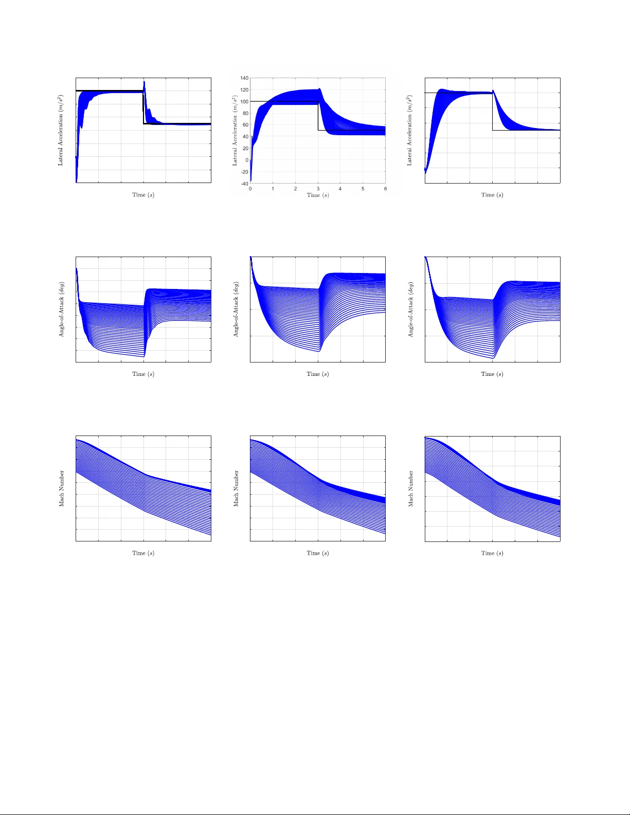
1 A Domain-Kno wledge-Aided Deep Reinforcement Learning Approach for Flight Control Design Hyo-Sang Shin, Shaoming He and Antonios Tsourdos Abstract —This paper aims to examine the potential of using the emerging deep r einfor cement learning techniques in flight control. Instead of learning from scratch, we suggest to leverage domain knowledge a vailable in lear ning to impro ve learning efficiency and generalisability . More specifically , the proposed approach fixes the autopilot structure as typical three-loop autopilot and deep reinf orcement learning is utilised to learn the autopilot gains. T o solve the flight control problem, we then formulate a Mark ovian decision process with a proper reward function that enable the application of reinf orcement learning theory . Another type of domain knowledge is exploited for defining the r eward function, by shaping refer ence inputs in consideration of important control objectives and using the shaped reference inputs in the reward function. The state-of- the-art deep deterministic policy gradient algorithm is utilised to learn an action policy that maps the observed states to the autopilot gains. Extensive empirical numerical simulations are performed to validate the proposed computational control algorithm. Index T erms —Flight Control, Deep reinfor cement learning, Deep deterministic policy gradient, Domain knowledge I . I N T R O D U C T I O N The main objectiv e of a flight controller for modern air vehicles is to track a given command in a fast and stable manner . Classical linear autopilot in conjunction with gain scheduling technique is one of widely-accepted frameworks for flight controller design due to its simplicity , local stability and ease of implementation [1]–[5]. This technique requires to linearise the airframe dynamics around several characteristic trim points and a static feedback linear controller is designed for each operation point. The controller gains are then online scheduled through a proper interpolation algorithm to cover the entire flight env elop. The systematic gain-scheduling approach provides engi- neers an intuitiv e framework to design simple and effecti ve controllers for nonlinear airframes. The issue is that its per- formance might be significantly degraded for a highly non- linear and coupled system in which the assumptions on the con ventional linear control theory could be violated. T o resolv e the issue, there hav e been extensi ve studies on other control Hyo-Sang Shin and Antonios Tsourdos are with the School of Aerospace, T ransport and Manufacturing, Cranfield University , Cranfield MK43 0AL, UK (email: { h.shin,a.tsourdos } @cranfield.ac.uk ) Shaoming He is with the School of Aerospace Engineering, Beijing Institute of T echnology , Beijing 100081, China (email: shaoming.he@bit.edu.cn ) and also with the School of Aerospace, T ransport and Manufacturing, Cranfield University , Cranfield MK43 0AL, UK (email: shaoming.he@cranfield.ac.uk ) “This work has been submitted to the IEEE for possible publication. Copyright may be transferred without notice, after which this version may no longer be accessible. ” theories, e.g., sliding mode control [6], [7], backstepping [8], adaptiv e control [9], [10], state-dependent Riccati equation (SDRE) method [11], [12] and H ∞ synthesis [13], [14]. Howe ver , each control method has its own advantages and limitations. For example, sliding mode control usually suffers from the chattering problem and therefore it is difficult to implement in practice. The backstepping autopilot requires to calculate the deriv atives of the virtual commands, which normally contain some information that cannot be directly measured. The implementation of SDRE controller requires to solve the complicated algebraic Riccati equation at each sampling instant. In a recent contribution [15], nonlinear flight controllers ha ve been prov ed to share the same structure with linear gain-scheduling controllers by properly adjusting the feedback gains and therefore might suffer from similar drawbacks: requiring partial model information in controller design. Thanks to the rapid development on embedded compu- tational capability , there has been an increasing attention on the development of computational control or numerical optimisation algorithms in recent years [16]. Unlike classical optimal autopilot, computational control algorithms generate the control input relies extensi vely on onboard computation and there is no analytic solution of any specific control law . Generally , computational control algorithms can be classified into two main categories: (1) model-based ; and (2) data-based. The authors in [17]–[19] le veraged model predictive control (MPC) to design a robust autopilot for agile airframes. The basic idea behind MPC is that it solves a constrained nonlinear optimisation problem at each time instant in a receding horizon manner and therefore shows appealing advantages in autopilot design. Except for MPC, bio-inspired numerical optimisation algorithms, e.g., genetic algorithm, particle swarm optimisa- tion, hav e also been reported for flight controller design in recent years [20], [21]. Most of the flight control algorithms discussed so far are model-based control algorithms: they are generally designed under the assumption that the model information is correctly known. It is clear that the performance of model-based optimi- sation approaches highly relies on the accuracy of the model utilised. For modern air vehicles that suffer from aerodynamic uncertainties, it would be more beneficial to dev elop data- based autopilot. Considering the properties of the autopilot problem, leveraging the reinforcement learning (RL) concept might be an attracti ve option for dev eloping a data-based control algorithm [22]–[28]. T o this end, this paper aims to examine the potential of using the emerging deep RL (DRL) techniques in flight controller 2 design. The problem is formulated in the RL framew ork by defining a proper Markovian Decision Process (MDP) along with a reward function. Since the problem considered is a continuous-time control problem, the state-of-the-art policy gradient algorithm, i.e., deep deterministic policy gradient (DDPG), is utilised to learn a deterministic action function. Previous works using RL or DRL to solve flight control problems mainly try to obtain networks, mapping from states directly to control actions [29]–[34]. As initial in vestig ations, we followed previous relev ant studies, applied them in an aerial vehicle model for low-le vel attitude control and ex- amined their performance. From the inv estigation, it is found that the learning effecti veness is generally an issue and it is extremely difficult to generalise, i.e. to train networks in a way providing a reasonable performance to different types of inputs to the control system. Our initial inv estigation suggests that this becomes more problematic in the aerial vehicle whose dynamics is statically unstable as a small change in the control command could result in an unstable response. An extensi ve literature survey indicated that there hav e some efforts to utilise prior or domain knowledge to improv e learning ef fecti veness, generalisation or both [35]–[39]. In [35], the authors proposed an learning architecture by util- ising background kno wledge, i.e., an approximate model of the behaviour , in reinforcement learning and demonstrated that this concept enables fast learning with reduced size of learning samples. The results of [36] rev ealed that using prior knowledge of the tasks can significantly boost the learning performance and generalisation capabilities. In [37]–[39], the authors suggested a particular structure that guides the learner by incorporating prior knowledge in supervised learning and reinforcement learning. This concept is prov ed to help increase the learning efficienc y and av oid getting stuck of the training process both in terms of training and generalisation error . The results from these studies strongly suggest that leveraging domain kno wledge can improve the learning effecti veness. T o this end, this paper focuses on dev eloping a DDPG- based control framew ork that exploits the domain kno wledge to enhance the learning efficienc y . The main contributions of the de velopment are three aspects: (1) W e develop a DDPG-based control frame work that utilises the domain knowledge, that is the control structure. As discussed, most of RL or Deep RL (DRL) based algorithms directly learn control actions from scratch that might hinder the learning ef ficiency . Unlike these typical algorithms, the proposed framew ork is formulated by fixing the autopilot structure. Under the problem formulated, DRL learns a deter- ministic action function that maps the observed engagements states to the autopilot gains. This enables the DRL-based control to enhance the learning efficienc y , retain the strengths of simple structure and improv e the performance of classical autopilot via learning. (2) The reference input to the control system is shaped by considering sev eral important criteria, e.g., rising time, damping ratio, overshooting, in control system design. Then, the shaped reference input is lev eraged in the rew ard function. This greatly simplifies the parameter tuning process in Multi- Objectiv e Optimisation (MOO). Note that there are many objectiv es required to be achiev ed in control system design and hence control problems are often expressed as an MOO problem. The proposed approach also allows the DRL-based control to resolve the particularity in applying RL/DRL to the control system design problem. (3) In the proposed DDPG-based control frame work, this paper suggests to use normalised observations and actions in the training process to tackle the issue with the scale of rew ards and networks. Our initial in vestigation indicated that different scales in states create different scales in rewards and networks. Consequently , the training becomes ineffecti ve, which will be shown via numerical simulations in Section VI-B. The numerical simulations confirm that this issue can be resolved by the normalisation. The proposed concepts and performance are examined through extensi ve numerical studies. The numerical analysis rev eals that the proposed DDPG autopilot guarantees satis- factory tracking performance and exhibits sev eral advantages against traditional gain scheduling approach. Robustness of the domain-knowledge-aided DDPG autopilot is also in ves- tigated by examining the performance of the proposed ap- proach against model uncertainty . The simulation results on the robustness examination confirm that the DDPG autopilot dev eloped is robust against model uncertainty . Also, relative stability of the proposed autopilot is numerically in vestigated and its results show that the proposed autopilot meets the typical design criteria on the phase and gain margins. The rest of the paper is or ganised as follows. Sec. II introduces of the basic concept of deep reinforcement learning. Sec. III presents nonlinear dynamics of airframes, followed by the details of the proposed computational flight control algorithm in Sec. IV . Finally , some numerical simulations and conclusions are offered. I I . D E E P R E I N F O R C E M E N T L E A R N I N G For the completeness of this paper, this section presents some backgrounds and preliminaries of reinforcement learning and DDPG. A. Reinforcement Learning In the RL framework, an agent learns an action policy through episodic interaction with an unknown environment. The RL problem is often formalised as a MDP or a partially observable MDP (POMDP). A MDP is described by a five- tuple ( S , O , A , P , R ) , where S refers to the set of states, O the set of observations, A the set of actions, P the state transition probability and R the reward function. If the process is fully observable, we hav e S = O . Otherwise, S 6 = O . At each time step t , an observation o t ∈ O is generated from the internal state s t ∈ S and giv en to the agent. The agent utilises this observation to generate an action a t ∈ A that is sent to the environment, based on specific action policy π . The action policy is a function that maps observations to a probability distribution ov er the actions. The en vironment then lev erages the action and the current state to generate the next state s t +1 with conditional probability P ( s t +1 | s t , a t ) and a scalar reward signal r t ∼ R ( s t , a t ) . For any trajectory in 3 the state-action space, the state transition in RL is assumed to follow a stationary transition dynamics distribution with conditional probability satisfying the Markov property , i.e., P ( s t +1 | s 1 , a 1 , · · · , s t , a t ) = P ( s t +1 | s t , a t ) (1) The goal of RL is to seek a policy for an agent to interact with an unknown environment while maximising the expected total re ward it receiv ed over a sequence of time steps. The total reward in RL is defined as the summation of discounted rew ard as R t = N X i = t γ i − t r i (2) where γ ∈ (0 , 1] denotes the discounting factor . Giv en current state s t and action a t , the expected total rew ard is also known as the action-value function Q π ( s t , a t ) = E π [ R t | s t , a t ] (3) which satisfies a recursive form as Q π ( s t , a t ) = E π [ R ( s t , a t ) + γ E π [ Q π ( s t +1 , a t +1 )]] (4) Therefore, the optimal policy can be obtained by optimising the action-value function. Howe ver , directly optimising the action-value function or action-value function requires accu- rate model information and therefore is difficult to implement with model uncertainties. Model-free RL algorithms relax the requirement on accurate model information and hence can be utilised e ven with high model uncertainties. B. Deep Deterministic P olicy Gradient For the autopilot problem, the main goal is to find a deterministic actuator command that could dri ve the air vehicle to track the target lateral acceleration command in a rapid and stable manner . Since this is a continuous control problem, we utilise the the model-free policy gradient RL approach to learn a deterministic function that directly maps the states to the actions, i.e., the action function is updated by follo wing the gradient direction of the value function with respect to the action, thus termed as policy gradient. More specifically , the state-of-the-art policy-gradient solution, DDPG proposed by Google Deepmind [40], is lev eraged to dev elop a com- putational lateral acceleration autopilot for an air vehicle. DDPG is an Actor-Critic method that consists of two main function blocks: (1) Critic ev aluates the giv en policy based on current states to calculate the action-value function; (2) Actor generates polic y based on the ev aluation of critic. DDPG utilises two different deep neural networks, i.e., actor network and critic network, to approximate the action function and the action-value function. The basic concept of DDPG is shown in Fig. 1. Denote A µ ( s t ) as the deterministic policy , which is a function that directly maps the states to the actions, i.e., a t = A µ ( s t ) . Here, we assume that the action function A µ ( s t ) parameterised by µ . In DDPG, the actor function is optimised by adjusting the parameter µ toward the gradient of the expected total rew ard as [40] ∇ a t Q w ( s t , A µ ( s t )) = ∇ µ A µ ( s t ) ∇ a t Q w ( s t , a t ) (5) Actor (Provide Control Policy) Critic (Evaluate Control Policy) En vironment Reward Output Observation Perf ormance Evaluation Action Fig. 1. Basic concept of DDPG. where Q w ( s t , a t ) stands for the action-value function, which is parameterised by w . The parameter µ is then updated by moving the policy in the direction of the gradient of Q w in a recursive way as µ t +1 = µ t + α µ ∇ µ A µ ( s t ) ∇ a t Q w ( s t , a t ) (6) where α µ refers to the learning rate of the actor network. Similar to Q-learning, DDPG also utilises the temporal- difference (TD) error δ t in approximating the error of action- value function as δ t = r t + γ Q w ( s t +1 , A µ ( s t +1 )) − Q w ( s t , a t ) (7) DDPG utilises the square of TD error as the loss function L ( w ) in updating the critic network, i.e., L ( w ) = δ 2 i (8) T aking the partial deriv ative of L ( w ) respect to w giv es ∇ w L ( w ) = − 2 δ i ∇ w Q w ( s t , a t ) (9) The parameter w is then updated using gradient descent by following the negati ve gradient of L ( w ) as w t +1 = w t + α w δ t ∇ w Q w ( s t , a t ) (10) where α w stands for the learning rate of the critic network. One major issue of using deep neural networks in RL is that most neural network optimisation algorithms assume that the samples for training are independently and identically distributed. Ho wever , this assumption is violated if the training samples are directly generated by sequentially exploring the en vironment. T o resolve this issue, DDPG leverages a mini batch buf fer that stores the training samples using the ex- perience replay technique. Denote e t = ( s t , a t , r t , s t +1 ) as the transition experience of the t th step. DDPG utilises a buf fer D with its size being |D | to store transition experiences. DDPG stores the current transition e xperience in the buf fer and deletes the oldest one if the number of the transition e xperience reaches the maximum value |D | . At each time step during training, DDPG uniformly draws N transition experience samples from the buf fer D and utilises these random samples to train actor and critic networks. By utilising the experience buf fer, the critic network is updated as ∇ µ J ( A µ ) = 1 N N X i =1 ∇ µ A µ ( s i ) ∇ a t Q w ( s i , a i ) µ t +1 = µ t + α µ ∇ µ J ( A µ ) (11) 4 Fig. 2. The longitudinal dynamics model and parameter definitions. W ith N transition experience samples, the loss function in updating the critic network now becomes L ( w ) = 1 N N X i =1 δ 2 i (12) The parameter of the critic network is updated by gradient decent as ∇ w L ( w ) = 1 N N X i =1 δ i ∇ w Q w ( s i , a i ) w t +1 = w t + α w ∇ w L ( w ) (13) Notice that the update of the action-v alue function is also utilised as the target value as shown in Eq. (7), which might cause the di ver gence of critic network training [40]. T o address this problem, DDPG creates one target actor network and one target critic network. Suppose the additional actor and critic networks are paramterised by µ 0 and w 0 , respectively . These two target networks use soft update, rather than directly copying the parameters from the original actor and critic networks, as µ 0 = τ µ + (1 − τ ) µ 0 w 0 = τ w + (1 − τ ) w 0 (14) where τ  1 is a small updating rate. This soft update law shares similar concept as low-frequency learning in model reference adaptiv e control to improve the robustness of the adaptiv e process [41], [42]. The soft-updated two target networks are then utilised in calculating the TD-error as δ t = r t + γ Q w 0  s t +1 , A µ 0 ( s t +1 )  − Q w ( s t , a t ) (15) W ith very small update rate, the stability of critic network training greatly improv es at the expense of slo w training process. Therefore, the update rate is a tradeof f between training stability and conv ergence speed. The detailed pseudo code of DDPG is summarised in Algorithm 1. I I I . N O N L I N E A R A I R F R A M E D Y N A M I C S M O D E L For the feasibility inv estigation of the proposed approach, this paper utilises the longitudinal dynamics model of a tail- controlled skid-to-turn airframe in autopilot design [11], as shown in Fig. 2. For simplicity , we assume that the air vehicle Algorithm 1 Deep deterministic policy gradient 1: Initialise the actor and critic networks with random weights µ and w 2: Initialise the target actor and critic networks with weights µ 0 ← µ and w 0 ← w 3: Initialise the experience buf fer D 4: for episode = 1: MaxEpisode do 5: for t = 1 : MaxStep do 6: Generate an action from the actor network based on current state a t = A µ ( s t ) 7: Add a random noise v t to the action for exploration a 0 t = a t + v t 8: Execute the action a 0 t and receiv e new state s t +1 and re ward r t 9: Store the transition experience e t = ( s t , a t , r t , s t +1 ) in the experience buf fer D 10: Uniformly draw N random samples e i from the experience buf fer D 11: Calculate the TD error δ i δ i = r i + γ Q w 0  s i +1 , A µ 0 ( s i +1 )  − Q w ( s i , a i ) 12: Calculate the loss function L ( w ) L ( w ) = 1 N N X i =1 δ 2 i 13: Update the critic network using gradient descent as ∇ w L ( w ) = 1 N N X i =1 δ i ∇ w Q w ( s i , a i ) w t +1 = w t + α w ∇ w L ( w ) 14: Update the actor network using policy gradient as ∇ µ J ( A µ ) = 1 N N X i =1 ∇ µ A µ ( s i ) ∇ a t Q w ( s i , a i ) µ t +1 = µ t + α µ ∇ µ J ( A µ ) 15: Update the target networks as µ 0 = τ µ + (1 − τ ) µ 0 w 0 = τ w + (1 − τ ) w 0 16: if the task is accomplished then 17: T erminate the current episode 18: end if 19: end for 20: end for 5 T ABLE I P H YS I C A L PA RA M E TE R S . Symbol Name V alue I yy Moment of Inertia 247.439 k g · m 2 S Reference Area 0.0409 m 2 d Reference Distance 0.2286 m m Mass 204.02 k g g Gravitational acceleration 9.8 m/s 2 T ABLE II A E RO DY NA MI C P O L Y NO M I A L C O E FFIC I E N TS . Symbol V alue Symbol V alue a a 0.3 a m 40.44 a n 19.373 b m -64.015 b n -31.023 c m 2.922 c n -9.717 d m -11.803 d n -1.948 is roll-stabilised, e.g., zero roll angle and zero roll rate, and has constant mass, i.e., after boost phase. Under these assumptions, the nonlinear longitudinal dynamics model can be expressed as ˙ α = QS mV ( C N cos α − C A sin α ) + g V cos γ + q ˙ q = QS d I y y C M ˙ θ = q γ = θ − α a z = V ˙ γ (16) where the parameters α , θ , γ and a z represent angle-of- attack, pitch attitude angle, flight path angle and lateral ac- celeration, respectively . In Eq. (16), m , g and V stand for mass, gravitational acceleration and velocity , respectiv ely . The variable Q represents the dynamic pressure, which is defined as Q = 0 . 5 ρV 2 with ρ being the air density . Additionally , the parameters S , d , I y y , and m denote reference area, diameter , moment of inertia, and mass, respectiv ely . The values of all physical parameters are detailed in T able I. The aerodynamic coef ficients C A , C N and C M are deter- mined as C A = a a C N = a n α 3 + b n α | α | + c n  2 − M 3  α + d n δ C M = a m α 3 + b m α | α | + c m  − 7 + 8 M 3  α + d m δ (17) where a i , b i , c i and d i with i = a, n, m are constants and the v alues are presented in T able II. The parameters M and δ represent Mach number and control fin deflection, respecti vely . The Mach number is subject to the following differential equation ˙ M = QS mV s ( C N sin α + C A cos α ) − g V s sin γ (18) where V s is the speed of sound. The actuator of an air vehicle is usually modelled by a second-order dynamic system as  ˙ δ ¨ δ  =  0 1 − ω 2 a − 2 ξ a ω a   δ ˙ δ  +  0 ω 2 a  δ c (19) where ξ a = 0 . 7 and ω a = 150 r ad/s denote the damping ratio and natural frequency , respectiv ely . The v ariable δ c represents the actuator command. Since the standard air density model is a function of height h , the following complementary function is introduced ˙ h = V sin γ (20) In autopilot design, the angle-of-attack α and the pitch rate ˙ θ are considered as the state v ariables. The lateral acceleration a z is considered as the control output v ariable and the actuator command δ c is regarded as the control input, that driv es the lateral acceleration to track a reference command a z ,c . I V . C O M P U T A T I O N A L L AT E R A L A C C E L E R A T I O N A U T O P I L OT A. Learning F ramework T o apply the DDPG algorithm in autopilot design, we need to formulate the problem in the DRL framework. One intuitiv e choice is to utilise the entire dynamics model, detailed in Eqs. (16)-(20), to represent the environment and directly learn the actuator command δ c during agent training process. Howe ver , this simple learning procedure has been shown to be ineffecti ve from our extensi ve test results. Our inv estigation suggests that it is mainly due to the nature of the vehicle dynamics: the considered longitudinal dynamics is statically unstable and therefore a small change in the control command could result in an unstable response. This hinders the learning effecti veness. Therefore, instead of learning the control action from scratch, we propose a new framew ork that utilises the domain knowledge to improv e the learning ef fectiv eness. T o this end, we fix the autopilot structure with several feedback loops and lev erage DDPG to learn the controller gains to implement the feedback controller . With this frame work, it is also expected that the learning efficienc y can be greatly improv ed. Notice that this concept is similar to fixed-structure H ∞ control methodology [43], [44]. Howe ver , our approach is a data-driven flight control algorithm and therefore has advantages against fixed-structure H ∞ method. Over the past sev eral decades, classical three-loop autopilot structures have been extensi vely employed for acceleration control for air vehicles due to its simple structure and ef fective- ness [1], [14], [15], [45], [46]. The classical three-loop autopi- lot is gi ven by a simple structure with two feedback loops, as shown in Fig. 3. The inner loop utilises a proportional-integral feedback of pitch rate and the outer loop lev erages proportional feedback of lateral acceleration. W ith this architecture, the autopilot gains K DC , K A , K I and K g are usually designed using linear control theory for several trim operation points individually . [46] compared various three-loop topologies and showed that the gains can be optimally derived by using the LQR concepts. Note that the three-loop autopilot is realised by 6 + - K DC K A + - K I s + - K g a z a z ,c q δ c Fig. 3. Three-loop autopilot structure. scheduling the gains with some external signals, e.g., angle- of-attack, Mach number , height in linear control. Due to this fact, implementing classical three-loop autopilot requires a look-up table and a proper scheduling algorithm. This fact inevitably increases the complexity of the controller and results in some approximation errors during the scheduling process. For modern air vehicles with large flight en velope, massiv e ad hoc trim operation points are required to guarantee the performance of gain-scheduling. This further increases the complexity of autopilot design. In recent study [15], there was an inv estigation to iden- tify the connection between linear and nonlinear autopilots through three-loop topology . This study rev ealed that non- linear autopilot shares the three-loop topology and the gains are parameter varying. The issue is that the performance of the non-linear controller can be significantly degraded with presence of system uncertainties, which could be the case in the modern air vehicles. This paper fixes the structure of the autopilot as three- loop topology . Note that we might be able to examine other autopilot topology to ov ercome the limitations of the con ven- tional one and e ven the autopilot topology could be subject of learning itself. W e will handle these points in our future study . T o address the issues with conv entional control theories discussed, this paper aims to utilise DDPG to provide a direct mapping from scheduling variables to autopilot gains, i.e., K DC = f 1 ( α, M , h ) K A = f 2 ( α, M , h ) K I = f 3 ( α, M , h ) K g = f 4 ( α, M , h ) (21) where f i with i = 1 , 2 , 3 , 4 are nonlinear functions. In other words, we suggest to directly train a neural net- work that provides nonlinear transformations from scheduling variables α , M , h , to autopilot gains K DC , K A , K I , K g . B. Pr oblem F ormulation T o learn the autopilot gains using DDPG, we need to formulate the problem in the RL framew ork by constructing a MDP with a proper rew ard function. 1) MDP definition: The dynamics of angle-of-attack, pitch angle, pitch rate, Mach number and height, shown in Eqs. (16)- (20), constitutes the environment, which is fully characterised by the system state s t = ( α, q , θ , M , h ) (22) Agent (Flight Control System) Flight V ehicle Reward Observation Action Fig. 4. Information flow of the proposed RL framework. As stated before, the aim of DDPG here is to learn the autopilot gains. For this reason, the agent action is naturally defined as a t = ( K DC , K A , K I , K g ) (23) From Eq. (20), it can be noted that the autopilot gains are functions of angle-of-attack, Mach number and height and these three variables are directly measurable from onboard sensors. For this reason, the agent observation is defined as o t = ( α, M , h ) (24) which gi ves a partially observable MDP . Note that the DDPG algorithm is applicable to partially observable MDP , as shown in [47]. It is worthy pointing out that we can also include pitch angle and pitch rate in the observation vector during training. Howe ver , increasing the dimension of observation will increase the difficulty for the training process as more complicated network for function approximation is required. The relativ e kinematics (16)-(20), environmental state (22), agent action (23), agent observation (24), together with a proper reward function, constitute a complete MDP formu- lation of the autopilot problem. The conceptual flowchart of the proposed flight control RL framew ork is shown in Fig. 4. 2) Rewar d function shaping: The most challenging part of solving the autopilot design problem using DDPG is the devel- opment of a proper reward function. Notice that the primary objectiv e of an acceleration autopilot is to drive the air vehicle to track a giv en acceleration command in a stable manner with acceptable transient as well as steady-state performance. In other words, the rew ard function should consider necessary time-domain metrics, e.g., rising time, overshoot, damping ratio, steady-state error , in an integrated manner . This means that the reward function should be designed as a weighted sum 7 T ABLE III H Y PE R - P A RA M E T ER S I N S H AP I N G T H E R E W A R D F U N CT I O N . k a k δ a z, max ˙ δ max 1 0 . 1 100 1 . 5 of sev eral individual objectiv es, which, by default, poses great difficulty on tuning the weights of dif ferent metrics. This paper proposes to resolve this issue by utilising another domain knowledge, that is the desired performance. In other words, we shape the original reference command, a z ,c , based on the desired performance and propose to track the shaped command ¯ a z ,c rather than the original reference command. The shaped command ¯ a z ,c satisfies the following two properties: (1) The shaped command is the output of a reference system; (2) The reference system has desired time-domain charac- teristics. This approach also enables alleviation of the particularity in applying RL/DRL to the control system design problem. One of the main objecti ves of the tracking control is to minimise the tracking error , that is the error between the reference command and actual output. If the tracking error is directly incorporated into the reward function with a discounting factor between 0 and 1, the learning-based control algorithm will consider minimising the immediate tracking error is more or equally important than minimising the tracking error in the future. This might cause instability issue and is not well aligned with the control design principles. Shaping the command and defining the tracking error with respect to the shaped command can relax this mismatch between the RL and control design concepts. In consideration of the properties of a tail-controlled air- frame, we propose the following reference system ¯ a z ,c ( s ) a z ,c ( s ) = − 0 . 0363 s + 1 0 . 009 s 2 + 0 . 33 s + 1 (25) where the utilisation of an unstable zero naturally arises from the non-minimum phase property of a tail-controlled airframe. The proposed rew ard function considers tradeof f between tracking error and fin deflection rate as r t = − k a  a z − ¯ a z ,c a z , max  2 − k δ ˙ δ ˙ δ max ! 2 (26) where k a and k δ are two positive constants that quantify the weights of two different objectiv es; a z , max and ˙ δ max are two normalisation constants that enforce these two metrics in approximately the same scale. Note that the consideration of fin deflection rate is to constrain the maximum rate of the actuator to meet physical limits. The hyper -parameters in shaping the reward function are summarised in T able III. V . T R A I N I N G A D D P G A U T O P I L OT A G E N T Generally , training a DDPG agent inv olves three main steps: (1) obtaining training scenarios; (2) building the actor and critic networks; and (3) tuning the hyper parameters. T ABLE IV F L IG H T E N VE L O P . Parameter Minimum value Maximum value Angle-of-attack α − 20 ◦ 20 ◦ Height h 6000 m 14000 m Mach number M 2 4 T ABLE V N E TW O R K L A Y E R S I ZE . Layer Actor network Critic network Input layer 3 (Size of observations) 7 (Size of observations + Size of actions) Hidden layer 1 64 64 Hidden layer 2 64 64 Output layer 4 (Size of action) 1 (Size of action-value function) 1) T raining scenarios: In this paper , we consider an air- frame with its flight en velop defined in T able IV. At the beginning of each episode, we randomly initialise the system states with values uniformly distributed between the minimum and the maximum values. This random initialisation allows the agent to explore the diversity of the state space. For all episodes, the vehicle is required to track a reference command a z ,c , which is defined as a step command with its magnitude being 100 m/s 2 . 2) Network construction: Inspired by the original DDPG algorithm [40], the actor and critic are represented by four- layer fully-connected neural networks. Note that this four-layer network architecture is commonly utilised in deep reinforce- ment learning applications [48]. The layer sizes of these two networks are summarised in T able V. Except for the actor output layer , each neuron in other layers is activ ated by a rectified linear units (Relu) function, which is defined as g ( z ) =  z , if z > 0 0 , if z < 0 (27) which provides faster processing speed than other nonlinear activ ation functions due to the linear relationship property . The output layer of the actor network is acti vated by the tanh function, which is giv e by g ( z ) = e z − e − z e z + e − z (28) The benefit of the utilisation of tanh activ ation function in actor network is that it can prev ent the control input from saturation as the actor output is constrained by ( − 1 , 1) . Since different autopilot gains hav e different scales, the output layer of the actor network is scaled by a constant vector [ K DC , max , K A, max , K I , max , K g , max ] T (29) where ( · ) max stands for the normalisation constant of variable ( · ) and the detailed values are presented in T able VI. As different observations have different scales and units, we normalise the observations at the input layers of the networks, thus providing unitless observations hat belong to approximately the same scale. This normalisation procedure is shown to be of paramount importance for our problems and 8 T ABLE VI N O RM A L I SATI O N C O NS TA NT S . α max M max h max K DC, max K A, max K I , max K g, max 20 ◦ 4 14000 3 0.05 100 2 helps to increase the training efficienc y . W ithout normalisa- tion, the average re ward function cannot conv erge and e ven shows diver gent patterns after some episodes. Denote ¯ ( · ) as the normalised version of variable ( · ) . The normalisation of observations is defined as ¯ α = α α max , ¯ M = M M max , ¯ h = h h max (30) where ( · ) max stands for the normalisation constant of variable ( · ) and the detailed values are presented in T able VI. Both actor and critic networks are trained using Adam optimiser with L 2 regularisation to address the over -fitting problem for stabilising the learning process. W ith L 2 regu- larisation, the updates of actor and critic are modified as L actor = J ( A µ ) + λ 2 L A 2 µ t +1 = µ t + α µ ∇ µ L actor (31) L critic = L ( w ) + λ 2 L C 2 w t +1 = w t + α w ∇ w L critic (32) where L A 2 and L C 2 denote the L 2 regularisation losses on the weights of the actor and the critic, respectively; λ 2 is the regularisation constant. T o increase the stability of the network training process, we utilise the gradient clip technique to constrain the update of both actor and critic networks. More specifically , if the norm of the gradient exceeds a giv en upper bound ρ , the gradient is scaled to equal with ρ . This helps to prev ent a numerical ov erflo w or underflow during the training process. 3) Hyper parameter tuning: Each episode during training is terminated when the number of time steps exceeds the maximum permissible value. All hyper parameters that are utilised in DDPG training for our problem are summarised in T able VII. Notice that the tuning of hyper parameters imposes great effects on the performance of DDPG and this tuning process is not consistent across different ranges of applications [48], [49], i.e., different works utilised dif ferent set of hyper parameters for their own problems. For this reason, we tune these hyper parameters for our autopilot design problem based on se veral trial and error tests. V I . R E S U LT S A. T raining Results In order to demonstrate the importance of the utilisation of reference command and domain knowledge, we also carry out simulations without using the shaped reference command and domain knowledge, i.e., learning from scratch. W ithout the shaped reference command, the reward function becomes r t = − k a  a z − a z ,c a z , max  2 − k δ ˙ δ ˙ δ max ! 2 (33) T ABLE VII H Y PE R PA RA M E T ER S E T T IN G S . Parameter V alue Parameter V alue Maximum permissible steps 200 Size of experience buf fer |D | 5 × 10 5 Maximum permissible episodes 1000 Size of mini-batch samples N 64 Actor learning rate α µ 10 − 3 Mean of exploration noise µ v 0 Critic learning rate α w 10 − 3 Initial variance of exploration noise Σ 1 0 . 1 L 2 regularisation constant λ 2 6 × 10 − 3 V ariance decay rate  10 − 6 Gradient upper bound ρ 1 Mean attraction constant β attract 0.15 Discounting factor γ 0.99 T arget network smoother constant τ 0.001 Sampling time T s 0 . 01 s The learning curves of the training process that lev erages domain kno wledge with random initial conditions are shown in the first ro w of Fig. 5, where Fig. 5 (a) is the result with shaped reference command and Fig. 5 (b) stands for the result without shaped reference command. The av erage rew ard is obtained by av eraging the episode reward within 30 episodes. From Figs. 5 (a) and (b), it can be clearly noted that the average rew ard of the proposed DDPG autopilot agent con verges to its steady-state value within 400 episodes, ev en with random initial conditions. Also, the utilisation of shaped reference command provides relativ ely faster con vergence speed and smoother steady-state performance. T o demonstrate this fact, Fig. 5 (c) provides the learning curves of learning from scratch for one fixed set point. From this figure, it is clear that the rew ard con ver gence speed of learning from scratch for one fixed set point is slower than that of the proposed approach for all random initial conditions in the flight en velope. This fact rev eals that the utilisation of domain knowledge significantly improv es the learning efficienc y . The reason is that the agent has already gained some experience by using the domain knowledge. T o in vestigate the importance of observ ation and action normalisation in training DDPG autopilot agent, we perform simulations with and without normalisation. Fig. 6 presents the comparison results of av erage reward conv ergence. From this figure, it is clear that utilising normalisation provides fast con vergence rate of the learning process and higher steady- state value of the av erage rew ard function: the a verage reward without normalisation is not con verged within 1,000 episodes, whereas the one with normalisation conv erges withing around 200 episodes. This means that leveraging observ ation and ac- tion normalisation helps to achiev e more efficient and effecti ve training process. The reason can be attributed to the fact that normalisation imposes equally importance on each element of the observation vector . Without normalisation, the scale difference between the elements varies in a great deal, e.g., the magnitude of height is much lager than that of angle-of- attack, and therefore prohibits effecti ve training of the actor and critic networks. 9 0 200 400 600 800 1000 -1500 -1000 -500 0 (a) With both domain knowledge and shaped refer- ence command 0 200 400 600 800 1000 1200 -3000 -2500 -2000 -1500 -1000 -500 0 (b) With only domain knowledge 200 400 600 800 1000 1200 -3000 -2500 -2000 -1500 -1000 -500 0 (c) Learning from scratch for one fixed set point Fig. 5. Comparisons of learning curves. 0 200 400 600 800 1000 -2000 -1500 -1000 -500 0 Fig. 6. Learning process comparison with respect to normalisation. B. T est Results T o test the proposed DDPG three-loop autopilot under various conditions, the trained agent is applied to some ran- dom scenarios and compared with classical gain scheduling approach. Note that the trained agent by learning from scratch is incapable to track reference signals that are different from the training process in our test. On the other hand, the trained agent by lev eraging domain knowledge can track reference signals which differ from those in the training process. There- fore, we only compare the performance of the proposed algorithm with classical gain-scheduling and training with domain knowledge, b ut without shaped reference command. The testing DDPG agent is chosen from the one that generates the largest episode rew ard during the training process, i.e., - 0.5527 (with the shaped reference command ) and -18.1761 (without the shaped reference command). The comparison results, including acceleration response, angle-of-attack history , Mach number profile and fin deflection angle, are presented in Figs. 7-10. From these figures, it can be observed that both the classical gain-scheduling and the proposed DDPG autopilots can somehow track the reference signal. Note that although the gains giv en a set point are designed to meet the typical autopilot design criteria for the gain scheduling, the set points are not optimally selected . Hence, response of the gain scheduling could be further improv ed by tuning the gains at more set points with more accurate model information. Howe ver , this is against with our arguments in Introduction and Section IV. As a comparison, the agent that learned from data without using the shaped ref- erence command provides poor transient performance, i.e., big undershoot at the beginning, and generates large performance variations ev en for the steady-state performance. Although the acceleration response under the proposed algorithm has larger ov ershoot than classical gain scheduling approach, the pro- posed autopilot shows more stable response with less response oscillations and smaller undershoot in all set points tested, as shown in Figs. 7. The test results reassure that leveraging domain knowledge can improve the learning effecti veness and generalisation. Fig. 10 shows that gain scheduling autopilot requires faster actuator response and larger maximum fin deflection angle. This means that the proposed algorithm requires less actu- ator resource in tracking the reference command than gain scheduling approach. Another characteristic of the proposed autopilot is that it provides a direct nonlinear mapping from the scheduling variables to controller gains and therefore does not require a look-up table for real implementation. Apart from the improved learning effecti veness and generalisation, the numerical demonstration results suggest that the proposed DDPG three-loop autopilot provides comparable results with sev eral advantages , compare to the classical gain scheduling approach, and could be a potential solution for three-loop autopilot design. C. Robustness Against Model Uncertainty The aerodynamic model of a tail-controlled airframe might experience inevitable uncertainties due to the change of centre of pressure or other en vironmental parameters. Moreover , the data used in training could be different from reality . Therefore, it is critical to inv estigate the robustness of the learning-based autopilot. T o inv estigate the rob ustness of the proposed DRL-based acceleration autopilot, we perform nu- merical simulations with uncertain models in this subsection. 10 0 1 2 3 4 5 6 -40 -20 0 20 40 60 80 100 120 (a) Gain-scheduling (b) DDPG without shaped reference command 0 1 2 3 4 5 6 -20 0 20 40 60 80 100 120 (c) DDPG with shaped reference command Fig. 7. Comparison results of acceleration response. 0 1 2 3 4 5 6 -16 -14 -12 -10 -8 -6 -4 -2 0 2 (a) Gain-scheduling 0 1 2 3 4 5 6 -20 -15 -10 -5 0 (b) DDPG without shaped reference command 0 1 2 3 4 5 6 -20 -15 -10 -5 0 (c) DDPG with shaped reference command Fig. 8. Comparison results of angle-of-attack. 0 1 2 3 4 5 6 3.1 3.2 3.3 3.4 3.5 3.6 3.7 3.8 3.9 (a) Gain-scheduling 0 1 2 3 4 5 6 3.1 3.2 3.3 3.4 3.5 3.6 3.7 3.8 3.9 (b) DDPG without shaped reference command 0 1 2 3 4 5 6 2.6 2.7 2.8 2.9 3 3.1 3.2 3.3 (c) DDPG with shaped reference command Fig. 9. Comparison results of Mach number . The aerodynamic coef ficients, detailed in T able II, are assumed to hav e random − 40% to +40% uncertainty . T o better show the robustness of the proposed control algorithm, these model uncertainties are not included in the training scenarios. The simulation results, including acceleration response, angle-of- attack, mach number and fin deflection angle, are presented in Fig. 11. From this figure, it can be clearly noted that the proposed DRL-based control algorithm provides satisfactory performance in the presence of aerodynamic model uncertain- ties: the model uncertainties only influence the transient effect and the steady-state tracking error remains at the same level as the case without aerodynamic uncertainty . These results clearly rev eal that the proposed control approach has strong robustness against model uncertainties. D. Relative Stability The relative stability is generally applied to examine the robustness of the control system within the linear control theory . Ho we ver , since the proposed DRL autopilot is non- linear and utilises the deep neural networks, it is hard to analyse the stability using classical linear control theory . T o this end, this paper suggests to inv estigate relativ e stability of the proposed autopilot based on their physical concepts: (1) the gain margin determines the maximum allow able gain increase while maintaining the control loop stability; (2) the phase margin denotes the maximum allowable time delay in 11 0 1 2 3 4 5 6 -10 -5 0 5 10 15 20 (a) Gain-scheduling 0 1 2 3 4 5 6 -10 -5 0 5 10 15 20 25 (b) DDPG without shaped reference command 0 1 2 3 4 5 6 0 5 10 15 20 25 (c) DDPG with shaped reference command Fig. 10. Comparison results of fin deflection angle. 0 1 2 3 4 5 6 -20 0 20 40 60 80 100 120 (a) Acceleration response 0 1 2 3 4 5 6 -30 -25 -20 -15 -10 -5 0 5 (b) Angle-of-attack 0 1 2 3 4 5 6 2.6 2.7 2.8 2.9 3 3.1 3.2 3.3 (c) Mach number 0 1 2 3 4 5 6 0 5 10 15 20 25 (d) Fin deflection angle Fig. 11. Simulation results of the proposed autopilot with model uncertainties. a z ,c k a z Input gain Autopilot Sensor Actuator Airframe Fig. 12. Method to determine gain margin. the control loop to guarantee stability . With these concepts in mind, the gain margin can by numerically computed as a z ,c e − ∆ ts a z Time delay Sensor Airframe Actuator Autopilot Fig. 13. Method to determine phase margin. follows: 1) Put an input gain k before the actuator , as shown in 12 Fig. 12, and find the maximum value of k that results in instability of the control loop. 2) The gain margin can then be determined as GM = 20 log( k ) ( dB ) (34) The phase margin can be also numerically determined as: 1) Put a time delay ∆ t before the actuator, as shown in Fig. 13, and find the maximum value of ∆ t that results in instability of the control loop. 2) Compute the gain crosso ver frequency f from the ob- tained time response (the frequency can be directly read from the oscillation response). 3) The phase margin can then be determined as PM = 360 f ∆ t ( deg ) (35) W e in vestigated relative stability in various set points and their the results are similar . Hence, we select three dif ferent heights: 6 km , 8 k m and 10 k m to demonstrate the results of relativ e stability examination. Notice that when performing relativ e stability analysis, the Mach number is time-v arying. The numerical tests of gain margin and phase margin are presented Figs. 14 and 15. From the results, we can readily obtain the result that the proposed autopilot satisfies typical design criteria: GM > 6 dB , PM > 45 ◦ V I I . C O N C L U S I O N W e hav e dev eloped a computational acceleration autopilot algorithm for a tail-controlled air vehicle using deep RL techniques. The domain knowledge is utilised to help increase the learning efficienc y during the training process. The state- of-the-art DDPG approach is lev eraged to train a RL agent with a deterministic action policy that maximises the expected total reward. Extensiv e numerical simulations v alidate the effecti veness of the proposed approach. Future work includes extending the proposed autopilot to other types of vehicles. V alidating the proposed computational autopilot algorithm under uncertain en vironment is also an important issue and requires further explorations. R E F E R E N C E S [1] P . Zarchan, T actical and strate gic missile guidance . American Institute of Aeronautics and Astronautics, 2012. [2] D. J. Stilwell, “State-space interpolation for a gain-scheduled autopilot, ” Journal of Guidance, Control, and Dynamics , vol. 24, no. 3, pp. 460– 465, 2001. [3] D. J. Stilwell and W . J. Rugh, “Interpolation of observer state feed- back controllers for gain scheduling, ” IEEE T ransactions on Automatic Contr ol , vol. 44, no. 6, pp. 1225–1229, 1999. [4] S. Theodoulis and G. Duc, “Missile autopilot design: gain-scheduling and the gap metric, ” Journal of Guidance, Contr ol, and Dynamics , vol. 32, no. 3, pp. 986–996, 2009. [5] H. Lhachemi, D. Saussi ´ e, and G. Zhu, “Gain-scheduling control design in the presence of hidden coupling terms, ” Journal of Guidance, Contr ol, and Dynamics , pp. 1872–1880, 2016. [6] A. Thukral and M. Innocenti, “ A sliding mode missile pitch autopilot synthesis for high angle of attack maneuvering, ” IEEE T ransactions on Contr ol Systems T echnolo gy , vol. 6, no. 3, pp. 359–371, 1998. [7] I. Shkolniko v , Y . Shtessel, D. Lianos, and A. Thies, “Robust missile autopilot design via high-order sliding mode control, ” in AIAA Guidance , navigation, and contr ol Conference and Exhibit , 2000. [8] G. Mattei and S. Monaco, “Nonlinear autopilot design for an asym- metric missile using robust backstepping control, ” Journal of Guidance, Contr ol, and Dynamics , vol. 37, no. 5, pp. 1462–1476, 2014. [9] A. J. Calise, M. Sharma, and J. E. Corban, “ Adaptive autopilot design for guided munitions, ” Journal of Guidance, Contr ol, and Dynamics , vol. 23, no. 5, pp. 837–843, 2000. [10] J. W ang, C. Cao, N. Hov akimyan, R. Hindman, and D. B. Ridgely , “ L 1 adaptiv e controller for a missile longitudinal autopilot design, ” in AIAA Guidance, Navigation and Control Conference and Exhibit , 2008, p. 6282. [11] C. Mracek, J. Cloutier , J. Cloutier , and C. Mracek, “Full en velope missile longitudinal autopilot design using the state-dependent riccati equation method, ” in Guidance, Navigation, and Control Confer ence , 1997. [12] C. P . Mracek, “SDRE autopilot for dual controlled missiles, ” IF AC Pr oceedings V olumes , vol. 40, no. 7, pp. 750–755, 2007. [13] H. Buschek, “Design and flight test of a robust autopilot for the iris- t air-to-air missile, ” Contr ol Engineering Practice , vol. 11, no. 5, pp. 551–558, 2003. [14] J.-H. Kim and I. H. Whang, “ Augmented three-loop autopilot structure based on mixed-sensiti vity H ∞ optimization, ” Journal of Guidance, Contr ol, and Dynamics , vol. 41, no. 3, pp. 751–756, 2017. [15] C.-H. Lee, B.-E. Jun, and J.-I. Lee, “Connections between linear and nonlinear missile autopilots via three-loop topology , ” Journal of Guidance, Control, and Dynamics , vol. 39, no. 6, pp. 1426–1432, 2016. [16] P . Lu, “Introducing computational guidance and control, ” Journal of Guidance, Contr ol, and Dynamics , vol. 40, no. 2, pp. 193–193, 2017. [17] W .-Q. T ang and Y .-L. Cai, “Predictive functional control-based missile autopilot design, ” Journal of Guidance, Control, and Dynamics , vol. 35, no. 5, pp. 1450–1455, 2012. [18] V . Bachtiar , T . M ¨ uhlpfordt, W . Moase, T . Faulwasser , R. Findeisen, and C. Manzie, “Nonlinear model predicti ve missile control with a stabilising terminal constraint, ” IF A C Pr oceedings V olumes , vol. 47, no. 3, pp. 457– 462, 2014. [19] V . Bachtiar, C. Manzie, and E. C. Kerrigan, “Nonlinear model-predictiv e integrated missile control and its multiobjectiv e tuning, ” Journal of Guidance, Contr ol, and Dynamics , vol. 40, no. 11, pp. 2961–2970, 2017. [20] K. Krishnakumar and D. E. Goldberg, “Control system optimization using genetic algorithms, ” Journal of Guidance, Control, and Dynamics , vol. 15, no. 3, pp. 735–740, 1992. [21] B. Karimi, I. Saboori, and M. Lotfi-Forushani, “Multiv ariable con- troller design for aircraft longitudinal autopilot based on particle swarm optimization algorithm, ” in 2011 IEEE International Conference on Computational Intelligence for Measur ement Systems and Applications (CIMSA) Proceedings . IEEE, 2011, pp. 1–6. [22] D. W ang, H. He, and D. Liu, “ Adaptiv e critic nonlinear robust control: A survey , ” IEEE T ransactions on Cybernetics , vol. 47, no. 10, pp. 3429– 3451, 2017. [23] Y . Li, Y . W en, K. Guan, and D. T ao, “Transforming cooling optimization for green data center via deep reinforcement learning, ” IEEE Tr ansac- tions on Cybernetics , 2019. [24] T . T an, F . Bao, Y . Deng, A. Jin, Q. Dai, and J. W ang, “Cooperative deep reinforcement learning for large-scale traffic grid signal control, ” IEEE T ransactions on Cybernetics , 2019. [25] W . Koch, R. Mancuso, R. W est, and A. Bestavros, “Reinforcement learning for uav attitude control, ” ACM T ransactions on Cyber-Physical Systems , vol. 3, no. 2, pp. 1–21, Feb 2019. [Online]. A vailable: http://dx.doi.org/10.1145/3301273 [26] Z. Huang, X. Xu, H. He, J. T an, and Z. Sun, “Parameterized batch reinforcement learning for longitudinal control of autonomous land ve- hicles, ” IEEE T ransactions on Systems, Man, and Cybernetics: Systems , vol. 49, no. 4, pp. 730–741, 2017. [27] L. Ding, S. Li, H. Gao, C. Chen, and Z. Deng, “ Adaptive partial rein- forcement learning neural network-based tracking control for wheeled mobile robotic systems, ” IEEE T ransactions on Systems, Man, and Cybernetics: Systems , 2018. [28] R. Cui, C. Y ang, Y . Li, and S. Sharma, “ Adaptiv e neural network control of auvs with control input nonlinearities using reinforcement learning, ” IEEE Tr ansactions on Systems, Man, and Cybernetics: Systems , vol. 47, no. 6, pp. 1019–1029, 2017. [29] S. Ferrari and R. F . Stengel, “Online adaptiv e critic flight control, ” Journal of Guidance, Control, and Dynamics , vol. 27, no. 5, pp. 777– 786, 2004. [30] R. Enns and J. Si, “Helicopter trimming and tracking control using direct neural dynamic programming, ” IEEE T ransactions on Neural networks , vol. 14, no. 4, pp. 929–939, 2003. 13 0 1 2 3 4 5 6 -20 0 20 40 60 80 100 120 (a) h = 6 k m 0 1 2 3 4 5 6 -20 0 20 40 60 80 100 120 140 (b) h = 8 k m 0 1 2 3 4 5 6 -20 0 20 40 60 80 100 120 140 (c) h = 10 k m Fig. 14. Relativ e stability analysis with gain margin. 0 1 2 3 4 5 6 -20 0 20 40 60 80 100 120 140 (a) h = 6 k m 0 1 2 3 4 5 6 -20 0 20 40 60 80 100 120 140 (b) h = 8 k m 0 1 2 3 4 5 6 -20 0 20 40 60 80 100 120 140 (c) h = 10 k m Fig. 15. Relativ e stability analysis with phase margin. [31] Y . Zhou, E.-J. van Kampen, and Q. P . Chu, “Incremental model based online dual heuristic programming for nonlinear adaptive control, ” Contr ol Engineering Practice , vol. 73, pp. 13–25, 2018. [32] Y . W ang, J. Sun, H. He, and C. Sun, “Deterministic policy gradient with integral compensator for robust quadrotor control, ” IEEE T ransactions on Systems, Man, and Cybernetics: Systems , 2019. [33] D. Xu, Z. Hui, Y . Liu, and G. Chen, “Morphing control of a new bionic morphing uav with deep reinforcement learning, ” Aerospace Science and T ec hnology , 2019. [34] H. Wu, S. Song, K. Y ou, and C. W u, “Depth control of model-free auvs via reinforcement learning, ” IEEE T ransactions on Systems, Man, and Cybernetics: Systems , vol. 49, no. 12, pp. 2499–2510, 2018. [35] D. Shapiro, P . Langley , and R. Shachter, “Using background knowledge to speed reinforcement learning in physical agents, ” in Pr oceedings of the fifth international conference on Autonomous agents , 2001, pp. 254– 261. [36] T . Chen, “Deep reinforcement learning with prior knowledge, ” Master’ s thesis, Pittsburgh, P A, May 2019. [37] C ¸ . G ¨ ulc ¸ ehre and Y . Bengio, “Knowledge matters: Importance of prior information for optimization, ” The Journal of Machine Learning Re- sear ch , vol. 17, no. 1, pp. 226–257, 2016. [38] D. Ferranti, D. Krane, and D. Craft, “The value of prior knowledge in machine learning of complex network systems, ” Bioinformatics , vol. 33, no. 22, pp. 3610–3618, 2017. [39] D. L. Moreno, C. V . Regueiro, R. Iglesias, and S. Barro, “Using prior knowledge to improve reinforcement learning in mobile robotics, ” Proc. T owar ds Autonomous Robotics Systems. Univ . of Essex, UK , 2004. [40] T . P . Lillicrap, J. J. Hunt, A. Pritzel, N. Heess, T . Erez, Y . T assa, D. Silver , and D. Wierstra, “Continuous control with deep reinforcement learning, ” arXiv preprint , 2015. [41] T . Y ucelen and W . M. Haddad, “Low-frequency learning and fast adaptation in model reference adaptiv e control, ” IEEE Tr ansactions on Automatic Contr ol , vol. 58, no. 4, pp. 1080–1085, 2012. [42] J. E. Gaudio, T . E. Gibson, A. M. Annaswamy , M. A. Bolender , and E. Lavretsky , “Connections between adaptiv e control and optimization in machine learning, ” arXiv preprint , 2019. [43] P . Apkarian and D. Noll, “Nonsmooth H ∞ synthesis, ” IEEE Tr ansac- tions on Automatic Contr ol , vol. 51, no. 1, pp. 71–86, 2006. [44] P . Apkarian, M. N. Dao, and D. Noll, “Parametric robust structured control design, ” IEEE Tr ansactions on Automatic Contr ol , vol. 60, no. 7, pp. 1857–1869, 2015. [45] N. Stein, H. W eiss, G. Hexner, and I. Rusnak, “Effect of missile config- uration and inertial measurement unit location on autopilot response, ” Journal of Guidance, Control, and Dynamics , pp. 2740–2745, 2016. [46] C. Mracek and D. Ridgely , “Missile longitudinal autopilots: comparison of multiple three loop topologies, ” in AIAA guidance, navigation, and contr ol conference and exhibit , 2005. [47] Y . Duan, X. Chen, R. Houthooft, J. Schulman, and P . Abbeel, “Bench- marking deep reinforcement learning for continuous control, ” in Inter- national Conference on Machine Learning , 2016, pp. 1329–1338. [48] P . Henderson, R. Islam, P . Bachman, J. Pineau, D. Precup, and D. Meger , “Deep reinforcement learning that matters, ” in Thirty-Second AAAI Confer ence on Artificial Intelligence , 2018. [49] R. Islam, P . Henderson, M. Gomrokchi, and D. Precup, “Reproducibil- ity of benchmarked deep reinforcement learning tasks for continuous control, ” arXiv preprint , 2017. Hyo-Sang Shin receiv ed his BSc on aerospace engineering from Pusan National Univ ersity in 2004 and gained an MSc on flight dynamics, guidance and control in Aerospace Engineering from KAIST and a PhD on cooperati ve missile guidance from Cranfield University in 2006 and 2010, respectiv ely . He is currently a Professor of Guidance, Control and Navigation Systems and Head of Autonomous and Intelligent Systems Group at Cranfield University . His current research interests include multiple tar- get tracking, adaptiv e and sensor-based control, and distributed control of multiple agent systems. 14 Shaoming He recei ved his BSc and MSc degrees in Aerospace Engineering from Beijing Institute of T echnology , in 2013 and 2016, respectiv ely , and a PhD in Aerospace Cranfield Univ ersity . He is cur- rently an associate professor in School of Aerospace Engineering at Beijing Institute of T echnology . His research interests include multi-target tracking, UA V guidance and trajectory optimization. Antonios Tsourdos obtained a MEng in electronic, control and systems engineering from the Univ ersity of Sheffield (1995), an MSc in systems engineering from Cardiff Univ ersity (1996), and a PhD in non- linear robust missile autopilot design and analysis from Cranfield University (1999). He is a Professor of Control Engineering with Cranfield University , and was appointed Head of the Centre for Cyber- Physical Systems in 2013. He was a member of the T eam Stellar , the winning team for the UK MoD Grand Challenge (2008) and the IET Innovation A ward (Category T eam, 2009).