Acoustic Scene Classification: A Competition Review

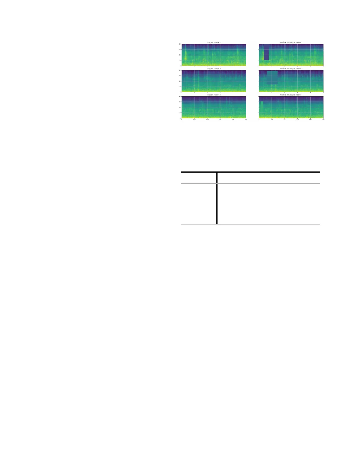
A COUSTIC SCENE CLASSIFICA TION: A COMPETITION REVIEW Shayan Gharib 1 , Honain Derrar 1 , Daisuke Niizumi 2 , T uukka Senttula 1 , J anne T ommola 1 , T oni Heittola 1 , T uomas V irtanen 1 , Heikki Huttunen 1 1 Lab . of Signal Processing, T ampere Univ ersity of T echnology , T ampere, Finland 2 Balmuda Inc., T okyo, Japan ABSTRA CT In this paper we study the problem of acoustic scene classi- fication, i.e., cate gorization of audio sequences into mutually exclusi ve classes based on their spectral content. W e describe the methods and results discovered during a competition or- ganized in the context of a graduate machine learning course; both by the students and e xternal participants. W e identify the most suitable methods and study the impact of each by per- forming an ablation study of the mixture of approaches. W e also compare the results with a neural netw ork baseline, and show the improv ement over that. Finally , we discuss the im- pact of using a competition as a part of a univ ersity course, and justify its importance in the curriculum based on student feedback. Index T erms — Acoustic Scene Classification, Data Aug- mentation, Kaggle, DCASE 1. INTR ODUCTION Humans are capable of understanding the en vironment by listening to the sounds surrounding them. One of the ma- jor research areas in computational auditory scene analysis (CASA) is acoustic scene classification (ASC) [1]. ASC at- tempts to classify digital audio signals into mutually exclusi ve scene categories, which can be e.g., an indoor en vironment (such as home ) or an outdoor en vironment (such as park ) [2]. It should be noted that this problem is different from a sound e vent detection (SED) task. In particular , SED attempts to classify , and detect the start and end points of sound e vents. Moreov er , sound ev ents may be o verlapping unlike the acous- tic scene classes, which are mutually exclusi ve. ASC can be applied in man y areas; including mobile robot navigation sys- tems [3] and conte xt-aware de vices [4], such as an automat- ically mode-switching smart phones according to the current acoustic en vironment [5]. In the sequel, we describe a pool of methods for solving the ASC problem, cro wdsourced during a two-month compe- This w ork w as partially funded by the Academy of Finland project 309903 CoefNet and ERC Grant Agreement 637422 EVER YSOUND. Au- thors also thank CSC–IT Center for Science for computational resources. tition organized as a mandatory part of a graduate level uni- versity course with almost 200 students. Moreo ver , the com- petition w as or ganized on the Kaggle InClass platform and was open for everyone, thus attracting talented researchers also outside the uni versity student community . Here, we de- scribe the common approaches that seemed to be of greatest benefit to the top teams, and attempt to synthesize a complete framew ork of ASC system adopting the best practices of this large cro wd of expert participants. The rest of the paper is organized as follows. In Section 2, we will revie w related literature, including the classical Hid- den Markov Model based approaches all the way until more recent deep learning based works. In Section 3, we will de- scribe the competition data, specifically tailored for this pur- pose. Section 4 presents the collection of successful methods, ranging from data augmentation to ensemble av eraging, deep learning and semi-supervised training. Finally , in Section 5, we discuss the importance of hands-on e xperience in educa- tion in general, and the role of a competition as part of the computer science curriculum in particular . 2. RELA TED WORK Giv en the huge variability of acoustic en vironments, the prac- tical approach is to gather a data set with a finite set of rele- vant categories and collect audio recordings from each. The resulting supervised classification task [2] is then well defined assuming the relev ance and validity of the data collection. As usual, compared to the manual engineering of acoustic indica- tors, learning algorithms can better handle the vast complexity and variability within the data [6]. One of the earliest approaches to A CS [7] in volves the use of feature extraction techniques used earlier in speech analysis and auditory research, coupled with Recurrent Neu- ral Networks (RNNs) and a K-Nearest-Neighbor criterion to construct a mapping between the feature space and the sound ev ent category . Later, researchers have used Hidden Marko v Models (HMM) that allow to take into account also the tem- poral unfolding of events within a sound sample. This is im- portant as using the temporal context of sound spectral com- ponents clearly improv es recognition accuracy . More recently , with the de velopment of deep learning [8], neural network approaches in general and conv olutional neu- ral networks (CNNs) in particular hav e become the dominant research track in the field of ASC. For e xample, all of the top 10 submissions in competitions such as the DCASE [9] are based on a CNN-based classifier either alone or in conjunc- tion with other techniques. CNNs hav e enabled researchers to obtain great results in image classification tasks such as in [10, 11]. Follo wing this success, also audio recognition has been rev olutionized by their strength. Competitions and community campaigns are of great im- portance in attracting talented researchers and pushing the state-of-the-art methods further within a research field. In this regard, DCASE challenge [12] is one of the competitions that is active on related fields to computational analysis of sound ev ents and scene analysis, namely acoustic scene classifica- tion, sound ev ent detection, and audio tagging. It started in 2013 including two tasks and 18 international participants, and has grown to already 87 teams in 2016 with 4 dif ferent tasks. Another benefit of competitions such as DCASE is to pro vide a fair comparison, and a baseline dataset for re- searchers to work with, and make the results of their studies more concrete for others to compare with. Apart from DCASE, music information retrie val e valua- tion exchange (MIREX) is another campaign which has been activ e for more than a decade, and co vered different tasks within the field of music information retriev al [13]. Even outside of research community , platforms such as Kaggle, CodaLab or CrowdAI hav e attracted research insti- tutions and companies to publish state-of-the-art challenges such as the recent T ensorFlow Speech Recognition challenge organized by Google. Moreov er , this opportunity is a ben- eficial practice not only for researchers b ut for people from outside of research community as well to extend and share their knowledge in a publicly accessible website. 3. COMPETITION SETUP AND D A T A The competition w as org anized in the conte xt of a two month graduate machine learning course in January-February 2018 on the Kaggle InClass platform, which is free for educati onal use. The course had over 200 participants that were split into groups of four students each (total 45 teams). More- ov er , the competition was open for ev eryone, and ev entually 69 teams participated; one third of all teams outside the uni- versity . The dataset (described below in more detail) features 15 ASC classes, and the performance metric for ranking the teams was the prediction accuracy ( i.e., ho w many percent of the audio samples were predicted correctly). In total, there were ov er 700 submissions from the teams. W e arranged a new dataset, TUT Acoustic Scenes 2017 Features 1 for crowdsourcing new approaches to acoustic 1 https://doi.org/10.5281/zenodo.1324390 scene classification. The goal was to have an easy to use, yet descriptiv e, dataset that would enable large scale adoption. Namely , many of the lar gest datasets ( e.g ., Google AudioSet) are challenging for a large scale adoption due to their sheer size and their dynamic nature (a collection of references to audio files, which may disappear ov er time). The dataset contains similar material to TUT Acoustic Scenes 2017 dataset [14, 15], used in the DCASE2017 acous- tic scene classification challenge [9]. Both datasets are com- posed from same pool of original audio recordings, but exact audio segments selected for the datasets dif fer . The acoustic material consists of binaural recordings from 15 acoustic scenes: lakeside beach, bus, cafe/restaur ant, car , city center , forest path, gr ocery stor e, home, library , metr o station, of fice, urban park, r esidential ar ea, train, and tram . Multiple recordings of 3-5 minutes length were captured from each scene class, and each recording was done in a different location to ensure high acoustic variability . Complete details on data recording procedure can be found in [16], although it should be noted that we only use a subset of the features of the complete set. In order to simplify the adoption of the dataset, we de- cided to exclude the pipeline for feature extraction from raw audio, and release the dataset only as acoustic features. More specifically , we e xtracted the log mel-energy features in 40 mel bands for each in 40 ms window (50% hop) for each 10- second long audio segment. Each 10-second recording is thus represented as a 40 × 501 feature matrix (40 frequency bins from 501 time points). The log mel-energy features were se- lected as they hav e shown to be among the most informativ e for this type of classification problem (see e.g ., [17]). 3.1. Development and evaluation sets The dataset consists of development set and evaluation folds. The de velopment set was released with ground truth, whereas the ev aluation set was released without true class labels. The participants may submit their predictions for the ev aluation set two times each day and the competition platform e valu- ates the accuracy . Moreover , the e valuation set is divided into public leaderboar d and private leaderboar d subsets (in Kag- gle terminology) with a 50/50 ratio. The participants see their score for the public leaderboard subset immediately; but the final team ranking is based on the hidden priv ate leaderboard subset, whose results are disclosed only when the competition ends. The three folds—de velopment (75%), public leader- board (12.5%) and pri vate leaderboard (12.5%)—correspond to the more common concepts of training, validation and test folds with the intention to discourage optimization ag ainst the test set. In absolute quantities, the development set contains 4500 audio segments with a length of 10 seconds, totaling 750 minutes of audio. The ev aluation set contains 1500 10- second audio segments, 250 minutes of audio in total. 3.2. Material selection Acoustic scenes hav e lar ge variability in the acoustic prop- erties, and due to limited amount of recordings and record- ing locations, extra care has to be taken to make the sets of the dataset balanced. The equally balanced sets are essen- tial for making the development process deterministic for the participants; the system should perform relatively equally in dev elopment set, in public leaderboard subset, and in priv ate leaderboard subset. Original recordings were av eraged into single channel and cut into 10-second segments. Segments originating from the same recording were assigned into same set, either dev elop- ment or ev aluation, to make ev aluation setup more realistic. Our segment selection procedure was done independently for each scene class. In this process a large number of randomly selected set candidates were created and ranked based on ho w acoustically similar segments were selected to the sets (de- velopment and ev aluation). The candidate sets were created by first randomly assigning recordings to sets and then ran- domly selecting se gments from these recordings to fill the tar- get number of se gments for each set. For the dev elopment set, 300 segments were selected per scene class, and for e v alua- tion set 100 segments. The final sets were selected randomly among the top 25% with best acoustic similarity . Acoustic similarity between the sets w as determined by training a Gaussian Mixture model (GMM) for each set and measuring the Kullback-Leibler div ergence between them. First, mel-frequency cepstral coefficients (MFCCs) were e x- tracted in 40 ms windows (50% hop size) for each segment in the sets. These features were then aggregated ov er one second analysis window (50% hop size) by calculating mean and standard de viation within the analysis windo w . The ag- gregated features were pooled separately for the dev elopment and e valuation sets, and a Gaussian Mixture model (GMM) was trained for each (32 components). Distance between these two GMMs was then calculated using the empirical symmetric Kullback-Leibler di ver gence [18, 19]. Instead of the within-sequence accuracy , we wanted to measure the inter-sequence generalization as well; i.e., how well the the approaches generalize to completely unseen se- quences. T o this aim, each sequence is included in exactly one of the three folds. Also the sequence index for each de- velopment sample was provided in order to enable local inter- sequence benchmarking with the training data for the partici- pants. 4. METHODS In this section, we describe a collection of successful meth- ods used by the top teams of the competition and assess their importance in the final accuracies. Fig. 1 . Illustration of the effects of Random Erasing. T able 1 . Public scores obtained with random erasing and mixup augmentation with and without cyclic learning rate (CLR) scheduling. Combination CLR Random erasing Mixup Public leaderboard Delta from baseline Baseline No No No 75.33 % 0.0 Baseline + CLR Y es No No 72.13 % -3.2 Baseline + Random erasing No Y es No 75.47 % +0.13 Baseline + Mixup No No Y es 76.27 % +0.93 Baseline + All but CLR No Y es Y es 76.40 % +1.07 Baseline + All Y es Y es Y es 77.07 % +1.73 4.1. Data A ugmentation One of the challenges related to deep neural networks is the large amount of data that they require to generalize properly . In order to address this, one may use different regularization approaches ( ` 1 and ` 2 penalty or dropout [20]) or data aug- mentation. In this regard, the top teams of the competition used two key augmentation approaches: r andom erasing [21] (closely related to cutout [22]), and mixup [23]. As in all augmen- tation, the idea behind both approaches is to synthesize new (hopefully realistic) samples from the training data to force the model to better learn the natural variability within the data. Augmentation by random erasing (and cutout) is inspired by dropout re gularization: Random erasing inserts blank rect- angles into the two-dimensional spectrogram (or image) at a randomly chosen size and location. The Random erasing was successfully used by the winning team, although the impro ve- ment is not as significant as that of other augmentation tech- niques. Howe ver , due to its simplicity it is easy to implement and make the model more robust against noise. Examples of random erasing effect are sho wn in Figure 1. A more important data augmentation technique is mixup [23]. In contrast to the aforementioned approaches, mixup merges training samples together instead of just distorting individual training samples. More specifically , consider two Fig. 2 . Illustration of mixup augmentation. Left: T wo original mel-spectrogram samples from the training set. Right: two mixtures of the original samples. randomly chosen training samples x i ∈ R P and x j ∈ R P with their corresponding class labels y i ∈ { 0 , 1 } C and y j ∈ { 0 , 1 } C in one-hot-encoded representation with P - dimensional features and C classes. Then, mixup constructs a ne w training sample ∼ x ∈ R P with target ∼ y ∈ R C as follo ws: ∼ x = λ x i + (1 − λ ) x j , ∼ y = λ y i + (1 − λ ) y j , where λ ∼ B eta ( α, α ) with hyperparameter α > 0 . This way we create mixtures of both input and output ending up at non-binary interpolated targets ∼ y . In T able 1, we compare the effects of the dif ferent data augmentation techniques on our baseline model which is a CNN based on the Alexnet [10] architecture. In addition to the augmentation techniques, we also e valuate the ef fect of using cyclic learning rate scheduling [24]—a significant com- ponent used by the best teams. As sho wn in the table, using random erasing and mixup without cyclic learning rate (CLR) improv es the accuracy score by approximately 1% over the base-line model. When augmentation is combined with CLR the accuracy is im- prov ed an additional 0.7%. 4.2. Model Fusion Many of the best teams used model fusion to combine differ - ent classifiers. A nov el idea disco vered during competition is to integrate model fusion with K -fold cross-validation. T o tackle the problem of domain adaptation, each fold consists of exclusi ve recording location identifiers. K models are trained using sub-sampled training data, and the entire procedure re- sults in not only the accuracy estimate, but an ensemble of models, as well. The models may then be used to predict labels and confidences for the test data, and fused together either with majority vote or a veraging the confidences. As an example, the con volutional architecture of one of the winning teams consists of four con volutional layers, fol- lowed by a layer of Gated Recurrent Units (GR Us) and a soft- max layer at the output. W ithout any augmentation, this struc- ture results in a score of 74.66% on the public leaderboard. If the model is trained separately fiv e times for 5-fold cross- validation, a straightforward majority v ote among the 5 dif- ferent instances yields a significant improv ement (78.93% on public leaderboard) ov er the baseline approach. W ith mixup augmentation, the accuracy further increases to 79.73% thus confirming the positiv e impact of data augmentation tech- niques in this context, as well. 4.3. Network Architectur es Apart from custom network designs, many teams used net- works familiar from image recognition context. Most impor- tantly , the VGG16 network structure [11] is successful with spectral data. Here, the teams use an instance of VGG16 pre- trained with the ImageNet dataset [25], but substitute all pre- trained dense layers with randomly initialized fully-connected layers (of dimension 4096, for example). Discarding the orig- inal dense layers is preferred, as the con volutional pipeline is not sensiti ve to the input dimensions (unlike the subsequent dense layers). The data only needs to be replicated along the ”color” axis to mak e the spectrogram dimensions simi- lar to those of a color image; e .g., the spectrogram of size 40 × 501 is replicated three times to a tensor with dimensions 40 × 501 × 3 . This architecture alone achieves an accurac y of 78.66% on the public leaderboard. 4.4. Semi-supervised Learning Semi-supervised learning is commonly used to inte grate large masses of inexpensi ve unlabeled data with smaller amount of expensi ve labeled data. In competitions, the natural approach for improving the accuracy is to train a semi-supervised model with the unlabeled test dataset. Although this ap- proach is not applicable in real time systems, it gi ves v aluable insight on how much domain adaptation could improv e the accuracy . A straightforward approach to semi-supervised learning consists of three stages: 1. T rain a model with the training dataset, 2. Predict labels for the test dataset, 3. Add the test samples with the predicted labels into the training set and retrain. Obviously , one may iterate the abov e procedure more than once, or add only those samples that were classified with high confidence ( e .g., with > 50 % confidence). As an example, one of the top teams applied this approach repeatedly three times reaching about 4.5% impro vement compared to a base- line model. T able 2 . Adv anced feature engineering approaches added on top of the baseline model with augmentation (baseline = best result of T able 1). Method Public LB Delta from base model Base-line model only 77.07 % 0.0 + T emporal av eraging 77.60 % +0.53 + Background subtraction 81.60 % +4.53 Fusion of the abov e 84.13 % +7.07 4.5. Prepr ocessing Finally , several manually engineered feature engineering pipelines were discov ered. Among the most successful ones are the following. T emporal averaging : This technique adds a layer at the beginning of the neural network pipeline to collapse the tem- poral dimension aw ay: In other words, we av erage each fre- quency bin over all time points, transforming the 40 × 501 - dimensional input into 40 -dimensional vector . By doing so, we emphasize on the influences of frequency bins and com- pletely ignore the temporal changes of sounds. Backgr ound subtraction: This preprocessing step normal- izes each frequenc y bin by subtracting the mean of each sam- ple. As a result, the mean o ver each 10 second sample be- comes zero, emphasizing the temporal patterns of lo w-ener gy frequency bins otherwise masked by high-ener gy bins. The effect of these preprocessing steps is studied in T a- ble 2. The top row shows the accuracy of the baseline model with augmentation and CLR (see T able 1). If we preprocess the data using temporal av eraging, we can see minor improve- ment (+0.53 %). On the other hand, using background sub- traction instead, results in a significant improvement (4.53 %) ov er the baseline. Moreover , fusing the three models together (plain baseline, baseline with temporal av eraging and baseline with background subtraction) impro ves the accuracy ev en fur- ther , with a net accuracy increase of 7.07 %. 5. EDUCA TIONAL V ALUE The competition was a mandatory part of a graduate le vel pattern recognition course. Therefore, a valid question is whether the competition adds v alue to the course and whether the students feel they actually learned something during the course of the competition. The overall satisfaction for the course was high. The stu- dents are required to submit a numerical ev aluation for gen- eral satisfaction of the course organization (grading: 1 = low- est, 5 = highest). The av erage grade of 110 respondents was 4.35, and none of the students gave a grade less than three. These both indicate that the course in general was very well liked. Of course, the competition is only one part of the course, so we also wanted to in vestigate the ef fect of the com- petition to the ov erall satisfaction. T o this aim, we analyzed the verbal feedback gi ven by the students. The v erbal feedback is fed into two sections: ”What worked well during the course?” and ”How would you im- prov e the course”; i.e., the verbal answers are grouped into positiv e and negati ve responses. The competition was men- tioned in 30.4 % of the positi ve responses and in 16.7 % of the ne gati ve ones. Moreover , the neg ativ e feedback regarding the competition was exclusiv ely organizational; e.g ., regard- ing team formation, timetables, or GPU av ailability . Qualitativ ely , the feedback can be categorized into a few broad groups as follows (with some examples translated to English by the authors). Scalability . Unlike traditional project works, the compe- tition is less limited and allows experimentation with an un- limited number of ways. Examples of feedback from this cat- egory include the follo wing: ”...the Kaggle competition let those with time and motivation to push themselves and learn as much as possible . ” ”The competition was an excellent motivator , which does not necessarily requir e huge amount of time. ” Reflectivity . An important aspect of student motiv ation comes from reflecting the skills of an indi vidual against those of the others. In an online competition, a participant receives the feedback immediately and gets an immediate (although noisy) feedback for the performance. Examples of feedback from this category include the follo wing: ”Really , ther e was a desir e to impr ove the score due to a live comparison with the others. ” Motivation. Many students felt that the competition is mo- tiv ating and allows them to learn real hands-on skills, includ- ing the following. ”The competition or ganized during the course was very motivating and at least I learned the most ther e. ” 6. CONCLUSION In this paper , we hav e described an implementation of a ma- chine learning competition in acoustic scene classification. Primarily , the competition was opened internally for students, but was also open to ev eryone and did successfully attract par- ticipants from all over the world. As a result, we described a collection of components that contributed to a successful re- sult. It is noteworth y , that none of the methods are limited to audio only . Indeed, man y approaches (cutout, mixup, etc.) were originally proposed for image data, and some—to t he best of our knowledge—not applied to audio before. In total, the competition attracted 69 teams with altogether ov er 700 submissions. Roughly one third of the teams were outside the student group, which increases the moti vation among stu- dents: the competition is not just about one course. Student feedback also suggests that gamification can be a significant part of modern higher level education, while simultaneously progressing also the state of the art in research. 7. REFERENCES [1] Y . Han, J. Park, and K. Lee, “Con v olutional neural networks with binaural representations and background subtraction for acoustic scene classification, ” W orkshop on Detection and Classification of Acoustic Scenes and Events , 2017. [2] D. Barchiesi, D. Giannoulis, D. Stowell, and M.D. Plumbley , “ Acoustic scene classification: Classifying en vironments from the sounds they produce, ” Signal Processing Ma gazine, IEEE , vol. 32, no. 3, pp. 16–34, May 2015. [3] S. Chu, S. Narayanan, C.-C.J. Kuo, and M.J. Mataric, “Where am I? Scene recognition for mobile robots using audio fea- tures, ” in Multimedia and Expo, 2006 IEEE International Con- fer ence on , July 2006, pp. 885–888. [4] B. Schilit, N. Adams, and R. W ant, “Context-aware computing applications, ” in F irst W orkshop on Mobile Computing Systems and Applications, 1994. IEEE, 1994, pp. 85–90. [5] A.J. Eronen, V .T . Peltonen, J.T . T uomi, A.P . Klapuri, S. Fager- lund, T . Sorsa, G. Lorho, and J. Huopaniemi, “ Audio-based context recognition, ” IEEE T ransactions on Audio, Speech, and Langua ge Processing , vol. 14, no. 1, pp. 321–329, jan 2006. [6] T . Heittola, E. C ¸ akır , and T . V irtanen, “The machine learning approach for analysis of sound scenes and events, ” in Com- putational Analysis of Sound Scenes and Events , pp. 13–40. Springer , 2018. [7] N. Sawhney and P . Maes, “Situational awareness from envi- ronmental sounds, ” Pr oject Rep. for P attie Maes , 1997. [8] Y . LeCun, Y . Bengio, and G. Hinton, “Deep learning, ” Nature , vol. 521, no. 7553, pp. 436, 2015. [9] A. Mesaros, T . Heittola, A. Diment, B. Elizalde, A. Shah, E. V incent, B. Raj, and T . V irtanen, “DCASE 2017 challenge setup: T asks, datasets and baseline system, ” in Pr oceedings of the Detection and Classification of Acoustic Scenes and Events 2017 W orkshop (DCASE2017) , 2017, pp. 85–92. [10] A. Krizhevsk y , I. Sutskev er , and G.E. Hinton, “Imagenet classification with deep con volutional neural networks, ” in Advances in Neural Information Pr ocessing Systems 25 , pp. 1097–1105. 2012. [11] Karen Simonyan and Andrew Zisserman, “V ery deep conv o- lutional networks for large-scale image recognition, ” arXiv pr eprint arXiv:1409.1556 , 2014. [12] A. Mesaros, T . Heittola, E. Benetos, P . Foster , M. Lagrange, T . V irtanen, and M.D. Plumbley , “Detection and classifica- tion of acoustic scenes and e vents: Outcome of the dcase 2016 challenge, ” IEEE/A CM T ransactions on Audio, Speech, and Language Pr ocessing , vol. 26, no. 2, pp. 379–393, 2018. [13] J Stephen Downie, “The music information retrie v al ev alua- tion exchange (2005–2007): A window into music information retriev al research, ” Acoustical Science and T echnology , vol. 29, no. 4, pp. 247–255, 2008. [14] A. Mesaros, T . Heittola, and T . V irtanen, “TUT Acous- tic Scenes 2017, dev elopment dataset, ” https://zenodo. org/record/400515 , 2017. [15] A. Mesaros, T . Heittola, and T . V irtanen, “TUT Acoustic Scenes 2017, ev aluation dataset, ” https://zenodo.org/ record/1040168 , 2017. [16] A. Mesaros, T . Heittola, and T . V irtanen, “TUT database for acoustic scene classification and sound ev ent detection, ” in 24th Eur opean Signal Pr ocessing Conference 2016 (EUSIPCO 2016) , Budapest, Hungary , Aug 2016, pp. 1128–1132. [17] E. Cakir, G. Parascandolo, T . Heittola, H. Huttunen, and T . V ir- tanen, “Con volutional recurrent neural networks for poly- phonic sound event detection, ” IEEE/ACM T ransactions on Audio, Speech, and Language Pr ocessing , vol. 25, no. 6, pp. 1291–1303, June 2017. [18] T . V irtanen and M. Helen, “Probabilistic model based similar- ity measures for audio query-by-example, ” in Applications of Signal Pr ocessing to Audio and Acoustics, 2007 IEEE W ork- shop on , New Paltz, NY , USA, Oct 2007, pp. 82–85, IEEE Computer Society . [19] T . Heittola, A. Mesaros, D. Korpi, A. Eronen, and T . V irta- nen, “Method for creating location-specific audio textures, ” EURASIP Journal on Audio, Speech and Music Pr ocessing , 2014. [20] N. Srivasta v a, G. Hinton, A. Krizhevsky , I. Sutske ver , and R. Salakhutdinov , “Dropout: A simple way to prev ent neural networks from overfitting, ” The Journal of Machine Learning Resear ch , v ol. 15, no. 1, pp. 1929–1958, 2014. [21] Z. Zhong, L. Zheng, G. Kang, S. Li, and Y . Y ang, “Random erasing data augmentation, ” arXiv pr eprint arXiv:1708.04896 , 2017. [22] T . DeVries and G.W . T aylor , “Improved regularization of con volutional neural networks with cutout, ” arXiv pr eprint arXiv:1708.04552 , 2017. [23] H. Zhang, M. Cisse, Y .N. Dauphin, and D. Lopez-P az, “mixup: Beyond empirical risk minimization, ” in International Confer - ence on Learning Repr esentations , 2018. [24] L.N. Smith, “Cyclical learning rates for training neural net- works, ” in IEEE W inter Conference on Applications of Com- puter V ision (W ACV), 2017 . IEEE, 2017, pp. 464–472. [25] J. Deng, W . Dong, R. Socher , L. J. Li, K. Li, and L. Fei-Fei, “Imagenet: A large-scale hierarchical image database, ” in 2009 IEEE Conference on Computer V ision and P attern Recogni- tion , June 2009, pp. 248–255.