Flatness-based control of a two-degree-of-freedom platform with pneumatic artificial muscles

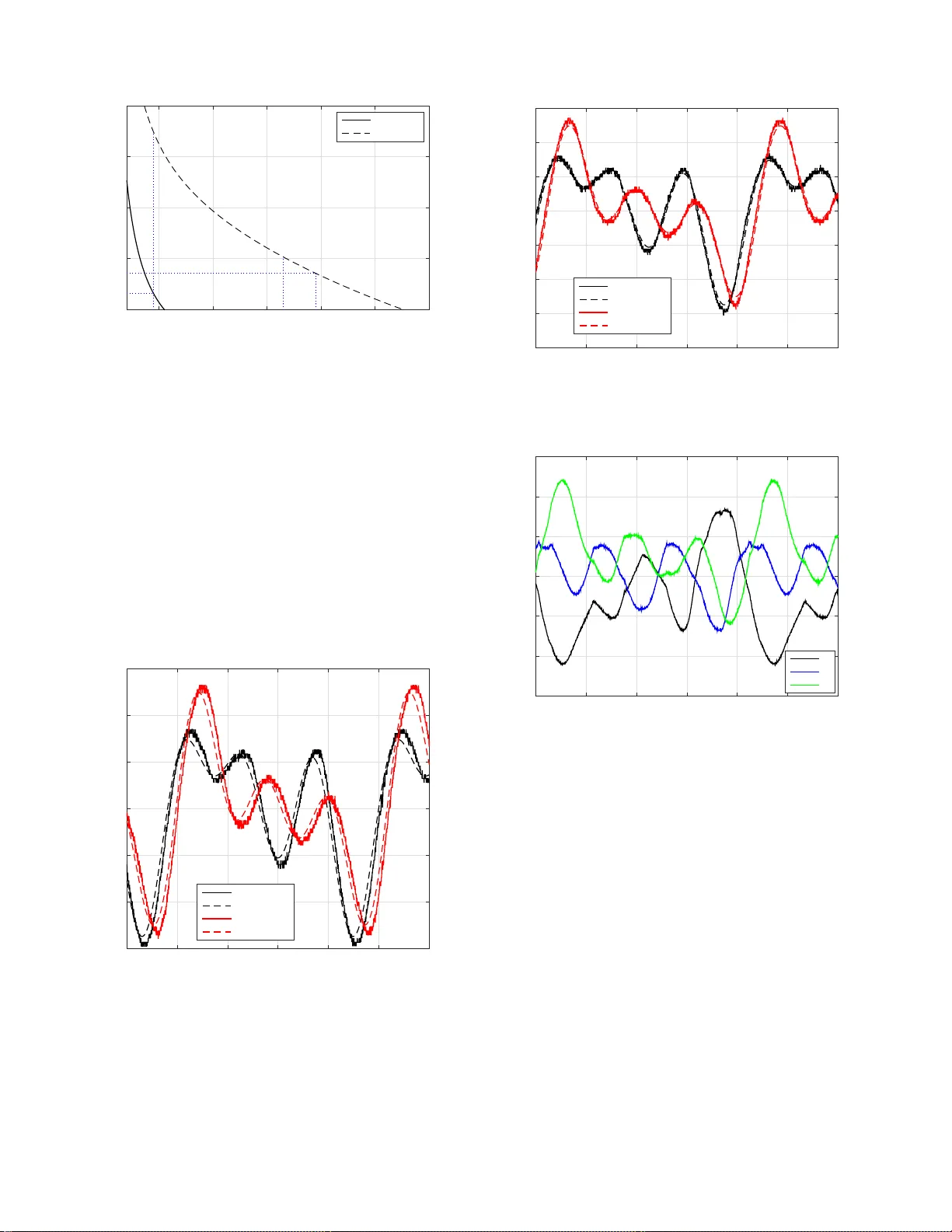
1 Flatness-based control o f a tw o-de gree- of-freedom platform with p n eumatic artificia l muscles David Bou S aba, Paolo Massioni, Eric Bideaux, a nd Xavier Brun Abstract —Pneumatic artificial muscles ar e a quite interesting type of actuators which hav e a very high power -to-weight and power -to-v olume ratio. Howe ver , thei r efficient use require s v ery accurate control methods which can take into account their complex dynamic, which is highly nonlinear . This paper consider a model of two-degr ee-of-freedom platform whose attitude is de- termined by three pneumatic muscles controlled b y servo valv es, which mimics a simpl ified version of a Stewart platform. For this testb ed, a model-based control approach is proposed, b ased on accurate first principle modeling of the muscles and th e platform and on a static model f or the serv o valv e. Th e employed control method is the so-called fl atness-based control i n troduced by Fliess. The paper first recalls the basics of th is control technique and then it shows how it can be appl i ed to the proposed experimental platfo rm; b eing flatness-based control an open- loop kind of control, a proportional-integral controller is added on top of it in order to add robustness wi t h respect to modelling errors and exter nal perturbations. At the end of the paper , the effectiveness of the proposed approach is shown by means of experimental results. A clear improv ement of the trackin g perfo rmance is visible co mpared to a simpl e proportional-integral controller . Index T erms —Pneumatic artificial muscles, nonlinear control, flatness. I . I N T R O D U C T I O N Pneumatic artificial muscles (P AMs) are a quite efficient type of actuato rs which feature high power-to-volume ratio, high pulling efforts at a relatively low price [7]. This makes their use quite interesting in many en gineering and ro botic applications, even if th e ir co ntrol is pro blematic due the non- linearity in th eir dyn amic model as well as fr o m the hysteresis pheno m ena wh ich they fea ture. Pneumatic artificial muscles produce a contraction ef fort when inflated , which is a non linear function of both the in ter- nal pr essure and the r elativ e contra ction o f its length . Many theoretical mod e ls o f P AMs can be fo und in the litera ture [7], [6], [15], and this paper will refe r to the results of exper- imental tests [3] that av erage out the h ysteresis phe nomena and ther efore can mode l the beh aviour very accurately . The subject of th is p aper is a stud y o f a two-degre e - of-free d om platform, actuated by thre e p n eumatic muscles. The objective is the synthesis of a model-b ased co n trol law allowing the tracking of a refer e nce tr a jectory for a wide operating range of the muscles. The platform is constrained to a limited o perating domain du e to mechan ical constraints and to the fact tha t the muscles generate only pulling efforts. Fu rthermor e, the system The authors are with Laboratoire Amp ` ere, UMR CNRS 5005, INSA de L yon, Uni versi t ´ e de L yon, 69621 V illeurbanne CEDEX, France. { david.bou-saba, paolo.massi oni, eric.bidea ux, xavier.brun } @ins a-lyon.fr . Corresponding author: P aolo Massioni, tel: +33(0)472 436035, fax: +33(0)472 438530. can be considere d as overactuated (th r ee actuators moving two degrees of freed om), w h ich r e quires a control a llo cation strategy . The contr ol of P AMs h as b een appr oached with several methods, which tr y to cope with the strong nonlinear ities of its dynamics. The appr o aches fou nd in the literature ar e mainly inherently no nlinear control m e th ods [2], [16]; slidin g mode controller s are one of the most commo n cho ices [1], [5], [1 3], also some times combine d with adap ti ve or n eural con trollers [14], [12], or backsteppin g [11]. Sliding mode controller s in fact provide enough robustness with respect to the d ynamical model which is considered as unce rtain. In this work, a flatness-based control [8] is propo sed, which exploits a model of all th e elements inv olved and which also solves the over-actuation p roblem at the same time. The robustness with respec t to model error s is pr ovided by cou pling the flatness-based co n troller with a pr o portion al-integral (PI) controller feeding b ack the erro r with respect to the refe rence trajectory . The paper is structur ed as follows. Section II intr oduces the notation used throu ghout the paper . Section II I descr ibes the model of the platform and o f all its elements, inc lu ding the pneumatic artificial muscles. Section IV shows that a proper choice of measur ements ma kes the platform a flat system, for which a flatness-based law is pr oposed. Section V concern s the problem of overactuation and how it is solved. At last, Section VI pro poses some exp erimental results whe r eas Section VII draws the conclusio ns o f the article. I I . N OTA T I O N A N D D E FI N I T I O N S Let R b e the set o f real number, and N the set of the strictly positive integers. For a m a trix A , A ⊤ denotes the transpo se. Giv e n two function s f ( x ) , g ( x ) ∈ R n , with x ∈ R n , let the Lie deriv ative o f f along g be defined as L g f ( x ) = ∂ f ( x ) ∂ x · g ( x ) . For ξ ∈ N , let L ξ g f ( x ) = ∂ L ξ − 1 g f ( x ) ∂ x · g ( x ) , with L 0 g f ( x ) = f ( x ) . For all signals x d ependin g from the tim e t , let x ( ξ ) indicate its ξ -th time deriv ative, i.e. x (1) = dx dt = ˙ x , x (2) = d 2 x dt 2 = ¨ x , etc. All th e symb ols con cerning the p neumatic mu scle platfo rm are defin e d in T ab le I. I I I . T H E P N E U M A T I C P L A T F O R M A. Descriptio n The pneuma tic platform studied in this p a per is represented in Fig. 1 and Fig . 2. It co nsists of a m etal plate fixed to a spherical hin ge on top of a vertical beam; three pneumatic muscles con tr olled by servov alves ar e attached to the plate at 2 P 0 Atmospheric pressure θ 0 W eave angle of the muscle at rest D 0 Diameter of the muscle at rest l 0 Length of the muscles at rest α Experimenta lly determined power coef ficient K Experimenta lly determined coeffici ent ε a Experimenta lly determined coeffici ent ε b Experimenta lly determined coeffici ent k Polytropi c index of air r Perfect gas constant T Air temperature R Muscle applicat ion point distanc e from center (constant ) J Mome ntum of inerti a about an horizontal axis (constant) φ 1 = − 90 ◦ Angular position of the 1 st m uscle (constan t) φ 2 = 30 ◦ Angular position of the 2 nd m uscle (constant) φ 3 = 150 ◦ Angular position of the 3 rd m uscle (constan t) θ x Angular position of the platform around x axis θ y Angular position of the platform around y axis P i Absolute pressure inside the i -th m uscle v i V oltage applied to the i -th servo valv e V i V olume of the i -th m uscle q i Mass flow into the i -th muscle ε i Contrac tion of the i -th muscle ε 0 Initia l contract ion of the muscle F i Force appli ed by the i -th the muscle Γ Perturbation torques T ABLE I S Y M B O L D E FI N I T I O N S . equally spac ed po ints. Due to the mu scles, and for simplicity , it can be considered that th e p latform has only two degre e s of f reedom, i.e. the two r o tational angle s ( θ x and θ y ) with respect to hor izontal axes p assing throu gh the hinge. An incli- nometer provides m e asurements o f such an gles, an d p ressure sensors are located in side eac h muscle. This platfo rm can be considered as a simplified version of a Stewart platfo rm, a test bench on wh ich co ntrol laws c an be tried and evaluated before m oving to more complex systems with more degrees of fre edom. Inclinometer Platform Pneumatic muscle Servovalve Pressure sensor Fig. 1. The experi mental platform. θ y θ x y x F 1 F 2 F 3 M 1 M 2 M 3 M 1 M 2 M 3 y x φ 1 φ 2 φ 3 z Fig. 2. Axonometric vie w and view from the top of the top plate, with definiti on of the axes x , y , z and the rotat ion angles θ x and θ y . M 1 , M 2 and M 3 are the attachment points of the three pneumatic artificial muscles. B. Mo d el This section rep orts the differential equations describing the system dyn amic and the d ifferent assumption s made. A mo re detailed description o f the com plete model of the system is presented in [4], with all the assumptions a n d explan ations (includin g those concern ing how the hysteresis ha s been taken into acco unt). The first elements to b e modeled are the pneumatic muscles, which ar e supposed to be id entical (they hav e th e same length at r est l 0 , the same initial contractio n ε 0 , etc.). Th e length contraction of each muscle ( i = 1 , 2 , 3 ) can be written as: ε i = R l 0 (cos φ i sin θ y − sin φ i sin θ x cos θ y ) + ε 0 (3) Subsequen tly , the rate of contraction of each m uscle is the time derivati ve of ε i , i.e. ˙ ε i = R l 0 h − ˙ θ x sin φ i cos θ x cos θ y + ˙ θ y (cos φ i cos θ y + sin φ i sin θ x sin θ y ) i (4)  ¨ θ x ¨ θ y  = M ( θ x , θ y )   F 1 F 2 F 3   + 1 J Γ (5) where the matrix M ( θ x , θ y ) is g iv en in equ ation (1) at the top of the n ext pag e. The ter m Γ = [Γ x , Γ y ] ⊤ contains the torques that will not be modelled (as an arbitrary choice) and will be left to the feedbac k co n trol to take c a r e of. Such terms are either du e to friction, or to gyr oscopic coupling s between the two axes, or to external f o rces acting on the platform. The friction ter ms ar e quite difficult to model exactly , whereas the gyroscop ic couplin g s are quite small d u e to the fact that the platform keeps always almost horizo ntal an d moves at rela tively low angu lar velocities. Th is allows writing the p latform around ea c h ax is a s d ecoupled , according to (5) above. Such an equation can also be written as  ¨ θ x ¨ θ y  = E ( θ x , θ y )  F 1 F 2  + G ( θ x , θ y ) F 3 + 1 J Γ (6) where the matr ices E ( θ x , θ y ) an d G ( θ x , θ y ) are given in equation (2) at the top of the n ext p age. This f o rm separates the effect o f the first two for ces with respect to F 3 , which makes it easier to appr oach the overactuatio n prob lem. 3 M ( θ x , θ y ) = R J  − si n φ 1 cos θ x cos θ y − si n φ 2 cos θ x cos θ y − si n φ 3 cos θ x cos θ y cos φ 1 cos θ y + sin φ 1 sin θ x sin θ y cos φ 2 cos θ y + sin φ 2 sin θ x sin θ y cos φ 3 cos θ y + sin φ 3 sin θ x sin θ y  (1)          E ( θ x , θ y ) = R J  − sin φ 1 cos θ x cos θ y − sin φ 2 cos θ x cos θ y cos φ 1 cos θ y + sin φ 1 sin θ x sin θ y cos φ 2 cos θ y + sin φ 2 sin θ x sin θ y  G ( θ x , θ y ) = R J  − sin φ 3 cos θ x cos θ y cos φ 3 cos θ y + s i n φ 3 sin θ x sin θ y  (2) In turn, each fo rce du e to pneu matic muscles can be modeled with th e so called quasi-static mo del [7], [4], [3] as F i ( P i , ε i ) = H ( ε i )( P i − P 0 ) + L ( ε i ) , (7) where L ( ε i ) = K ε i ( ε i − ε a ) ε i + ε b (8) and H ( ε i ) = π D 2 0 4  3 (1 − ε i ) α tan 2 θ 0 − 1 sin 2 θ 0  (9) with α , K , ε a and ε b experimentally deter mined co nstants. Considering that the operatin g range of th e servov alves is for 1 . 25 bar 6 P i 6 7 bar , the p ossible fo rces fo r each muscle are represented in Figure 3. Notice th a t on ly traction f orces are po ssible (the muscles cann ot push ) . Contraction ( ǫ i ) 0 0.05 0.1 0.15 0.2 0.25 Traction force (F i ) [N] 0 100 200 300 400 500 600 700 800 900 1000 P i = 1.25 bar P i = 2 bar P i = 3 bar P i = 4 bar P i = 5 bar P i = 6 bar P i = 7 bar Fig. 3. Traction force applied by a muscle as a function of the contract ion ε i and absolute pressure P i . The pr essure inside e a ch muscle is m odeled as ˙ P i = k rT V i ( ε i )  q i ( P i , v i ) − P i rT ∂ V ( ε i ) ∂ ε i ˙ ε i  (10) where k is th e p o lytropic ind ex of the gas, r the perf e ct gas constant, T the tem p erature (co nsidered constant), q i the mass flow o f gas, and V i the volume o f the muscle, for which the following formula has been pr oposed [4], [3] ∂ V ∂ ε i ( ε i ) = π 4 D 2 0 l 0  − 1 sin 2 θ 0 + ( α + 1) (1 − ε i ) α tan 2 θ 0  (11) where D 0 , l 0 are the diameter an d length of the muscle at re st, and θ 0 is the weave a n gle of the muscle fibers (a c o nstant). At last, the mass flow of gas q i entering each m uscle is a nonlinear fu n ction of the pressure in side the mu scle a n d the voltage v i fed to the servov alve. This fu nction is consider ed as static, and it can b e describe d by me ans of a poly nomial approx imation of experim ental data [10] (graphic a lly depicted in Figure 4). 7 6 Pressure (P i ) [bar] 5 4 3 2 1 -5 Voltage (v i ) [V] 0 -100 200 100 0 -200 5 Mass flow (q i ) [Nl/min] -150 -100 -50 0 50 100 150 Fig. 4. Mass flow of a servo v alv e as a function of vol tage v i and absolute muscle pressure P i . Considering that at each time instant, P i is measured by pressure sensors, it is possible to find the v i which gives the desired q i by a simple inv e r sion of the polyno mial function q i ( P i , v i ) . C. Contr o l ob jectives The aim of this testbed is to demo nstrate the ab ility to track any smo oth trajector y of θ x and θ y . Trajectories of this kin d can be cho sen as infinitely differentiable piece-wise polyno mial fu nction. The an gles of the platfo rms ( θ x , θ y ) are ph ysically con- strained to be in th e range [ − 15 ◦ , 15 ◦ ] . For these values, fo r the contraction s ε i the r anges are constrained with in [ − 0 . 03 , . 21] (the muscles need to be con tracted in o rder to apply a force) , for wh ich H ( ε i ) is never eq ual to 0 . I V . M O D E L A N A L Y S I S A N D C O N T RO L The accurate knowledge of the mo del allows the application of flatness-based contro l, at the co ndition of b eing able to prove tha t the system is flat. The relevant notio ns are recalled here. 4 A. Fla tness and flatness-ba sed con tr ol The notio n of flat system and flatness-b ased contro l for nonlinear systems have been intro duced in [8]. Basically , th e “flatness” is a prop erty o f a dyna m ical system and a cho ice of its outp ut y , as d e fin ed here. Definition 1 (F lat system - adapted fr om [8]): A d ynamical system of equ ations ˙ x = f ( x ) + g ( x ) u , with x ∈ R n , u = ∈ R m is flat if there exist an R m -valued map h , a n R n -valued map η , and an R m -valued map θ such that y = h ( x, u, u (1) , . . . , u ( ν ) ) (12) x = η ( y , y (1) , . . . , y ( ν − 1) ) (13) u = θ ( y , y (1) , . . . , y ( ν ) ) (14) for an app ropriate value of ν ∈ N . Th e output y is then called “flat ou tput”. The idea o f flatness can be explained briefly as follows. If one can choose as many output variables y i as inputs (the system is square), such th at it is po ssible to recover the state an d the inputs from the deriv atives of these output variables, then the system is flat a nd a flatness-based , op en loop con trol law can be derived b y system inv ersion (as explained later on). T wo fund amental conc e pts for sy stem in version a r e character istic index and co upling matrix. Definition 2 (Characteristic index): The character istic index of the i -th compo nent y i of y is the smallest ρ i ∈ N f or which L g j L ρ i − 1 f h i 6 = 0 for at least one value of j . Definition 3 (Coupling matrix): The couplin g matrix ∆( x ) is given by the expression: ∆( x ) =       L g 1 L ρ 1 − 1 f h 1 L g 2 L ρ 1 − 1 f h 1 . . . L g m L ρ 1 − 1 f h 1 L g 1 L ρ 2 − 1 f h 2 L g 2 L ρ 2 − 1 f h 2 . . . L g m L ρ 2 − 1 f h 2 . . . . . . . . . . . . L g 1 L ρ m − 1 f h m L g 2 L ρ m − 1 f h m . . . L g m L ρ m − 1 f h m       . (15) It can be shown th at       y ( ρ 1 ) 1 y ( ρ 2 ) 2 . . . y ( ρ m ) m       = ∆( x ) u +      L ρ 1 f h 1 L ρ 2 f h 2 . . . L ρ m f h m      . (16) The con trol law which has been app lied to the testbed is based on the following theo r em, which is a we ll-known result for wh ich no proof is necessary here. Theor em 4 (Adapted fr om [8]): I f a system of equations ˙ x = f ( x ) + g ( x ) u with u ∈ R m is flat (Definition 1) with respect to a flat o utput y = h ( x ) ∈ R m with ch aracteristic coefficients ρ i , and if the matrix ∆( x ) is invertible (at least locally), then it is possible to track a given smooth reference trajectory y ( t ) = h ( x ( t )) by em ploying the co ntrol law u = ∆( x ) − 1             y ( ρ 1 ) 1 y ( ρ 2 ) 2 . . . y ( ρ m ) m       −      L ρ 1 f h 1 L ρ 2 f h 2 . . . L ρ m f h m            . (17) It is possible to prove that with this state trajectory , the system’ s d ynamic of each y i is linear ( simp ly a chain of ρ i integrators). B. Comp lete state-space model The state of th e platf orm model c a n be chosen as x = [ x 1 , x 2 , x 3 , . . . x 7 ] ⊤ = [ θ x , θ y , ˙ θ x , ˙ θ y , P 1 , P 2 , P 3 ] ⊤ , whereas the input vector is u = [ q 1 , q 2 , q 3 ] ⊤ . By neglecting the perturb ation ter m Γ , the system dynamic can then be expr essed as fo llows . ˙ x = f ( x ) + g ( x ) u (18) where f ( x ) =                                 x 3 x 4 − cos x 1 cos x 2 sin φ 1 ( H ( ε 1 ) ( x 5 − P 0 ) + L ( ε 1 )) − cos x 1 cos x 2 sin φ 2 ( H ( ε 2 ) ( x 6 − P 0 ) + L ( ε 2 )) − cos x 1 cos x 2 sin φ 3 ( H ( ε 3 ) ( x 7 − P 0 ) + L ( ε 3 )) (cos φ 1 cos x 2 + sin φ 1 sin x 1 sin x 2 ) ( H ( ε 1 ) ( x 5 − P 0 ) + L ( ε 1 )) + (cos φ 2 cos x 2 + sin φ 2 sin x 1 sin x 2 ) ( H ( ε 2 ) ( x 6 − P 0 ) + L ( ε 2 )) + (cos φ 3 cos x 2 + sin φ 3 sin x 1 sin x 2 ) ( H ( ε 3 ) ( x 7 − P 0 ) + L ( ε 3 )) a ( ε 1 , ˙ ε 1 )( x 5 − P 0 ) a ( ε 2 , ˙ ε 2 )( x 6 − P 0 ) a ( ε 3 , ˙ ε 3 )( x 7 − P 0 )                                 , (19) g ( x ) = [ g 1 ( x ) , g 2 ( x ) , g 3 ( x )] with g 1 ( x ) =           0 0 0 0 b ( ε 1 ) 0 0           , g 2 ( x ) =           0 0 0 0 0 b ( ε 2 ) 0           , g 3 ( x ) =           0 0 0 0 0 0 b ( ε 3 )           (20) with        a ( ε i , ˙ ε i ) = − k V ( ε i ) ∂ V ( ε i ) ∂ ε i ˙ ε i b ( ε i ) = k rT V ( ε i ) (21) C. Flatn ess of the mod el The system is flat if a vector flat ou tput [ y 1 y 2 y 3 ] ⊤ , ac c ord- ing to (12), can b e fo und. Su ch flat output has to f ulfill bo th (13), i.e., it sho u ld be po ssible to express the state vector as a f unction o f its time der i vati ves, and (14), i.e. it should be possible to express the input a s a function o f its d eriv atives. This p aragraph shows that th e choice    y 1 = x 1 y 2 = x 2 y 3 = F 3 = H ( ε 3 )( x 7 − P 0 ) + L ( ε 3 ) (22) 5 actually works in m aking the sy stem flat. First con sid e r c ondition (13); x 1 , x 2 , x 3 and x 4 can be obtained d irectly from y 1 , y 2 and their first degre e time deriv atives. Once x 1 , x 2 , x 3 and x 4 are kn own, all ε i , H ( ε i ) and L ( ε i ) are determ ined as well. Since F 3 is an o u tput and H ( ε 3 ) 6 = 0 , x 7 is immed iately also determined . At last, x 5 and x 6 can be determine d f rom ˙ x 3 and ˙ x 4 if th e matrix  − cos x 1 cos x 2 sin φ 1 − cos x 1 cos x 2 sin φ 2 cos x 2 cos φ 1 + sin x 1 sin x 2 sin φ 1 cos x 2 cos φ 2 + sin x 1 sin x 2 sin φ 2  is in vertib le. T he determinan t o f this matrix is cos 2 x 2 cos x 1 (sin φ 2 cos φ 1 − sin φ 1 cos φ 2 ) which is never 0 in the range of θ x = x 1 , θ y = x 2 allowed f or th e platform (i. e . they never r each ± 9 0 ◦ ). Secondarily , consider condition (13); a ne c essary condition for this is that th e sum of the characteristic indices of the three outpu ts is the same a s th e numb e r of states, i.e. 7 . The computatio n of such indices lea d s to the f ollowing r e sults. • Output y 1 L g 1 y 1 = L g 2 y 1 = L g 3 y 1 = 0 ⇒ ρ 1 > 1 ; L f y 1 = x 3 ; L g 1 L f y 1 = L g 2 L f y 1 = L g 3 L f y 1 = 0 ⇒ ρ 1 > 2 ; L 2 f y 1 = ˙ x 3 = − cos x 1 cos x 2 (sin φ 1 ( H ( ε 1 )( x 5 − P 0 )+ L ( ε 1 )) + sin φ 2 ( H ( ε 2 )( x 6 − P 0 ) + L ( ε 2 ))+ sin φ 3 ( H ( ε 3 )( x 7 − P 0 ) + L ( ε 3 ))); L g 1 L 2 f y 1 = − sin φ 1 cos x 1 cos x 2 H ( ε 1 ) b ( ε 1 ) L g 2 L 2 f y 1 = − sin φ 2 cos x 1 cos x 2 H ( ε 2 ) b ( ε 2 ) L g 3 L 2 f y 1 = − sin φ 3 cos x 1 cos x 2 H ( ε 3 ) b ( ε 3 ) It can be po inted out that L g 1 L 2 f y 1 , L g 2 L 2 f y 1 and L g 3 L 2 f y 1 are never eq ual to 0 for the x 1 and x 2 within the valid range , so ρ 1 = 3 . • Output y 2 L g 1 y 2 = L g 2 y 2 = L g 3 y 2 = 0 ⇒ ρ 2 > 1; L f y 2 = x 4 ; L g 1 L f y 2 = L g 2 L f y 2 = L g 3 L f y 2 = 0 ⇒ ρ 2 > 2 ; L 2 f y 2 = ˙ x 4 = (cos φ 1 cos x 2 + sin φ 1 sin x 1 sin x 2 )( H ( ε 1 )( x 5 − P 0 ) + L ( ε 1 ))+(co s φ 2 cos x 2 +sin φ 2 sin x 1 sin x 2 )( H ( ε 2 )( x 6 − P 0 ) + L ( ε 2 )) + (cos φ 3 cos x 2 + sin φ 3 sin x 1 sin x 2 )( H ( ε 3 )( x 7 − P 0 ) + L ( ε 3 )); L g 1 L 2 f y 2 = (cos φ 1 cos x 2 + sin φ 1 sin x 1 sin x 2 ) H ( ε 1 ) b ( ε 1 ) L g 2 L 2 f y 2 = (cos φ 2 cos x 2 + sin φ 2 sin x 1 sin x 2 ) H ( ε 2 ) b ( ε 2 ) L g 3 L 2 f y 2 = (cos φ 3 cos x 2 + sin φ 3 sin x 1 sin x 2 ) H ( ε 3 ) b ( ε 3 ) Notice that L g 2 L 2 f y 2 can nev e r be zero in the valid range, as the fun ction z = cos φ 2 cos x 2 + sin φ 2 sin x 1 sin x 2 (23) plotted in Figur e 5 nev er reach es zero in this in terval. So ρ 2 = 3 . Fig. 5. V alue of z as function of x 1 = θ x and x 2 = θ y . • Output y 3 L g 1 y 3 = L g 2 y 3 = 0 ; L g 3 y 3 = b ( ε 3 ) H ( ε 3 ) 6 = 0 ⇒ ρ 3 = 1 . The necessary conditio n of ρ 1 + ρ 2 + ρ 3 = 7 is satisfied. The last step is to verify that the dec oupling matrix ∆ =   L g 1 L 2 f y 1 L g 2 L 2 f y 1 L g 3 L 2 f y 1 L g 1 L 2 f y 2 L g 2 L 2 f y 2 L g 3 L 2 f y 2 L g 1 y 3 L g 2 y 3 L g 3 y 3   (24) is in vertible . The expression of ∆ is made explicit in (25) at the top of the next page (with the shor thand notation of H i = H ( ε i ) , L i = L ( ε i ) , b i = b ( ε i ) ). The determina n t of this m a trix is | ∆ | = H 1 H 2 H 3 b 1 b 2 b 3 m with m = − sin φ 1 cos x 1 cos x 2 (cos φ 2 cos x 2 + sin φ 2 sin x 1 sin x 2 ) + s in φ 2 cos x 1 cos x 2 (cos φ 1 cos x 2 + sin φ 1 sin x 1 sin x 2 ) . The values of m as function of θ x and θ y in the valid interval are dep icted in Fig u re 6 According ly , | ∆ | 6 = 0 , so the deco upling matrix is in vertible over the o perating r ange and th e chosen output is proven to be flat. Fig. 6. V alues of m as function of θ x and θ y . 6 ∆ =   − sin φ 1 cos x 1 cos x 2 H 1 b 1 − sin φ 2 cos x 1 cos x 2 H 2 b 2 − sin φ 3 cos x 1 cos x 2 H 3 b 3 (cos φ 1 cos x 2 + sin φ 1 sin x 1 sin x 2 ) H 1 b 1 (cos φ 2 cos x 2 + s i n φ 2 sin x 1 sin x 2 ) H 2 b 2 (cos φ 3 cos x 2 + sin φ 3 sin x 1 sin x 2 ) H 3 b 3 0 0 H 3 b 3   (25) platform inclinometer flatness co ntroller pressure sensors muscle mo del + − + + PI in verse polynom ial m ap servov alves v i q i θ x,y P i F 3 θ x , ˙ θ x , ¨ θ x , ... θ x , θ y , ˙ θ y , ¨ θ y , ... θ y , F 3 , ˙ F 3 error desired q i experimental setup controller Fig. 7. Global control scheme. D. Con tr ol la w The platform can then be con trolled in op en-loop with the law q = ∆ − 1 ( x )       y ( ρ 1 ) 1 y ( ρ 2 ) 2 y ( ρ 3 ) 3    −   L 3 f y 1 L 3 f y 2 L f y 3      + ∆ − 1 ( x ) w (26) where y i is th e desired tr ajectory and w is an ad ditional contro l term. Due to the p resence o f the perturb ation terms which have bee n neglected ( Γ ), if w = 0 ther e will necessarily be a non -zero error ǫ i = y i − y i . Considering that the d ynamic of the system und er this law is just a chain of integrators, by imposing to w a fee dback law as a functio n o f the ǫ i closes the lo op. In this case, a propo rtional-integral contro ller (PI) has b een tune d. Figure 7 shows the overall contro l scheme. The flatness-b ased c o ntrol is for some aspects, quite similar to feedback linearisation control [9]. The main differences lie in the fact that flatn ess-based requ ires a specific choice o f flat output (wher eas f eedback linearisation can take any ou tput, assuming th e system is observable), and that it does no t require a kn owledge or measu re of the state variable. On the other hand, the baseline flatn ess-based control is feedf orward only , which req uires the in troduction of th e addition al f eedback term w . V . S O LV I N G T H E O V E R A C T UAT I O N It can be po inted out that th e p latform is overactu a ted, in the sense that th e three forces applied by the muscles are generating only two torques. T o tell it in anoth e r way , the av er age value of th e F i is irrelev an t for the platfo rm’ s dynamic; if a given F 1 = ˜ F 1 , F 2 = ˜ F 2 and F 3 = ˜ F 3 generate certain torques, then F 1 = ˜ F 1 + F 0 , F 2 = ˜ F 2 + F 0 and F 3 = ˜ F 3 + F 0 will g enerate the same torque s fo r any F 0 . On th e othe r hand, it is u seful to have thr ee muscles instead of two due to the fact that mu scles can on ly pull and no t pu sh, i.e. their for ce range is quite lim ited as shown by Fig ure 3. The cho ice o f F 3 as one of the flat outp ut can be then interpreted in th e light of th is fact: first of all, it would be impossible to resolve the state fr om th e output if one of the forces (o r pressure) is no t measur e d, as their effects on th e angles is the same up to a constant ter m. Secondarily , the flat co ntrol allows choosing the value of F 3 , which lets o ne choose the best value in or d er to let all the muscles b e in their valid f orce range. Consider that at each instant, th e ε i are deter mined by the in stantaneous geo m etry , wh ich implies that e a ch muscle has a lim ited interval of p ossible ap plicable forces (see Figure 8). One can find the intersection of su ch intervals an d call F min its m in imum and F max its m a x imum. Under the reasonable hypothesis that the platf orm turns slowly (in any case it is constrained to an gles smaller than 1 5 ◦ ), it can b e assumed that F 1 , F 2 and F 3 have to be close to th e equilibriu m values, i.e. F 1 ≈ F 2 ≈ F 3 . For this r eason, setting the refer ence for F 3 as F 3 = 1 2 ( F max ( ε 1 , ε 2 , ε 3 ) + F min ( ε 1 , ε 2 , ε 3 )) (27) giv es the best chances of having F 2 and F 3 within th e realisable inter val as well. For the experimen t in the next section, the referen c e fo r F 3 has b een determine d b y the law in (27). V I . E X P E R I M E N TA L R E S U LT S In order to assess the perf ormance of the prop o sed control approa c h , a n experime n t has been con ducted o n the platfor m. The pro posed flatn ess-based control coup led with PI ha s b een compare d to a PI contr oller , empirically tun ed to get the best ap parent p erform a n ces. Th e same r eference trajecto ry (a combinatio n of sinusoids) has been tested for b oth contro llers. Figure 9 repor ts the results f or the PI controller, wherea s Figure 10 shows the flatn ess-based co ntroller resu lts. It is 7 Contraction ( ǫ i ) 0 0.05 0.1 0.15 0.2 0.25 Traction force (F i ) [N] 0 150 300 450 600 P i = 1.25 bar P i = 7 bar F min F max ǫ 1 ǫ 3 ǫ 2 Fig. 8. For a give n position , the three contract ions ε i are giv en, so not all forces are possible for eac h muscle, but onl y those within the pressure range betwee n 1 . 25 and 7 bar . One can compute F max (the maximum force that all muscles can ex ert) and F max (the m inimum force that all muscles can ex ert). Settin g F 3 as the av erage betwee n these two allo ws all muscles to apply the desired forces and to maximise their range. apparen t fro m the p icture that the feed forward actio n added b y the flatn ess-based con trol greatly improves the tracking ability; in fact, it can b e com p uted th a t the ro ot mean squ are trackin g errors (for θ x and θ y respectively) are 0 . 51 an d 0 . 59 degrees for the PI ca se. W ith the flatn ess co n troller, these root me a n square erro rs becom e less than half, i.e. 0 . 25 and 0 . 29 d egrees respectively (co nsider also that the inclinometer s’ ou tput h as a q u antisation equivalent to 0 . 18 degree s). time [s] 0 5 10 15 20 25 30 degrees -6 -4 -2 0 2 4 6 θ x (measure) reference for θ x θ y (measure) reference for θ y Fig. 9. Traj ectory tracking with simple PI control. Figure 11 shows the ev o lution of th e pressur e s durin g the flatness-based contro ller test. Figu r e 1 2 shows the for ce o f the three m uscles durin g th e same test; rememb er that the referenc e for F 3 is deter mined with the overactuation- solving law pro posed in Section V. No tice that the f orces never saturate (and n either do th e voltages or the pressure) , which validates th e p r oposed strategy . time [s] 0 5 10 15 20 25 30 degrees -8 -6 -4 -2 0 2 4 6 θ x (measure) reference for θ x θ y (measure) reference for θ y Fig. 10. Traj ectory tracking with flatness-based control plus a PI. time [s] 0 5 10 15 20 25 30 bar 3.5 4 4.5 5 5.5 6 6.5 P 1 P 2 P 3 Fig. 11. Pressures insid e the pneumatic arti ficial muscles during the flatness- based control plus PI experi ment. V I I . C O N C L U S I O N This p a per has presented the successful a p plication o f a flatness-based controller to a platform featuring three P AMs. The experimental resu lts clearly show a better trajectory tr a ck- ing comp ared to a sim p le PI c ontroller . Futu r e research will look at the po ssibility of using P AMs for building a comp lete six-degree-of -freedo m Stewart platform , and con trolling it with the same appro ach. R E F E R E N C E S [1] H. Aschemann and D. Schindele . Sliding-mode cont rol of a hi gh-speed linea r axis driv en by pneumatic muscle actuators. IEEE T ransactions on Industrial E lect r onics , 55(11):3855–3864 , 2008. [2] D. X. Ba, T .Q. Dinh, and K.K. Ahn. An integrate d intell igent nonlinea r control met hod for a pneumatic artifici al muscle. IEEE /ASME T ransac- tions on Mechatr onics , 21(4):1835–1 845, 2016. [3] E . Bideaux, S. Sermeno Mena, and S. Sesmat. Parallel m anipulator dri ven by pne umatic muscles. In 8th Interna tional Confer ence on Fluid P ower (8th IFK) , Dresden, Germany , 2012. 8 time [s] 0 5 10 15 20 25 30 N 80 100 120 140 160 180 200 220 240 260 280 F 1 F 2 F 3 Fig. 12. Forces applied by the pneumatic artificial muscles (estimate d from the pressures and the contract ions) with flatness-based control plus a PI. [4] D. Bou Saba, E. Bideaux, X. Brun, and P . Massioni. A complet e model of a two degree of freedom platform actuated by three pneu- matic muscles elaborat ed for control synthesis. In BATH/ASM E 2016 Symposium on Fluid P ower and Mot ion Cont r ol , pages V001 T01A004– V001T01A004. American Society of Mechanica l Engineers, 2016. [5] D. Cai and Y . Dai. A s liding mode con trolle r for manipula tor dri ven by artifici al muscle actuato r . In Procee dings of the 2000 IEEE International Confer ence on Contr ol A pplica tions , pages 668–673. IEEE , 2000. [6] C.-P . Chou and B. Hannaford. Measurement and m odeling of McKibben pneumati c artificia l muscles. IEEE T ransactions on R obotics and Automat ion , 12(1):90– 102, 1996. [7] F . Daerden and D. Lefeber . Pneumatic artificia l muscles: actuat ors for robotics and automat ion. Eur opean journal of mechanica l and en vir onmental engineering , 47(1):11–21, 2002. [8] M. Fliess, J. L ´ evine, P . Martin, and P . Rouchon. Flatness and defect of non-linear s ystems: introductory theory and examples. Internati onal J ournal of Contro l , 61(6):1327– 1361, 1995. [9] A. Isidori. Nonlinear contr ol systems . Springer Science & Business Media, 2013. [10] O. Olaby , X. Brun, S. Sesmat, T . Redarc e, and E . Bideaux. Charac - teriza tion and modeling of a proportional value for control synthesis. In Proc eeding s of the JFPS Internati onal Symposium on Fluid P ower , volu me 2005, pages 771–776. The Japan Fluid Power System Society , 2005. [11] R.A. Rahman and N. Sepehri. Design and experimen tal ev aluation of a dynamical adapti ve backsteppi ng-slidin g mode control scheme for positioni ng of an antagonisti cally paired pneumatic artificial muscles dri ven actuati ng system. Internati onal Journal of Contr ol , pages 1–26, 2016. [12] R.M. Robinson, C.S. Kot hera, R.M. Sanner , and N.M. W ereley . Non- linea r control of robotic manipulat ors dri ven by pneumati c artific ial muscles. IEEE/ASME T ransacti ons on Mecha tr onics , 21(1):55–68, February 2016. [13] X. Shen. Nonlinea r model-based control of pneumati c artificia l muscle servo systems. Contr ol Engineerin g Practice , 18(3):311–317, 2010. [14] G.L . Shi and W . Shen. Hybrid control of a parallel platform based on pneumati c artificial muscles combining sliding m ode controller and adapti ve fuzzy CMA C. Contr ol Engineering Practi ce , 1(1):76–8 6, 2013. [15] B. T ondu and P . Lopez. Modeling and control of McKibben artific ial muscle robot actuators. Contr ol Systems, IEEE , 20(2):15– 38, 2000. [16] X. Zhu, G. T ao, B. Y ao, and J. Cao. Adapti ve robust posture control of parallel manipulato r dri ven by pneumatic muscles with redundancy . IEEE/ASME Tr ansactions on Mechat r onics , 13(4):441 –450, August 2008.