Transforming optimization problems into a QUBO form: A tutorial

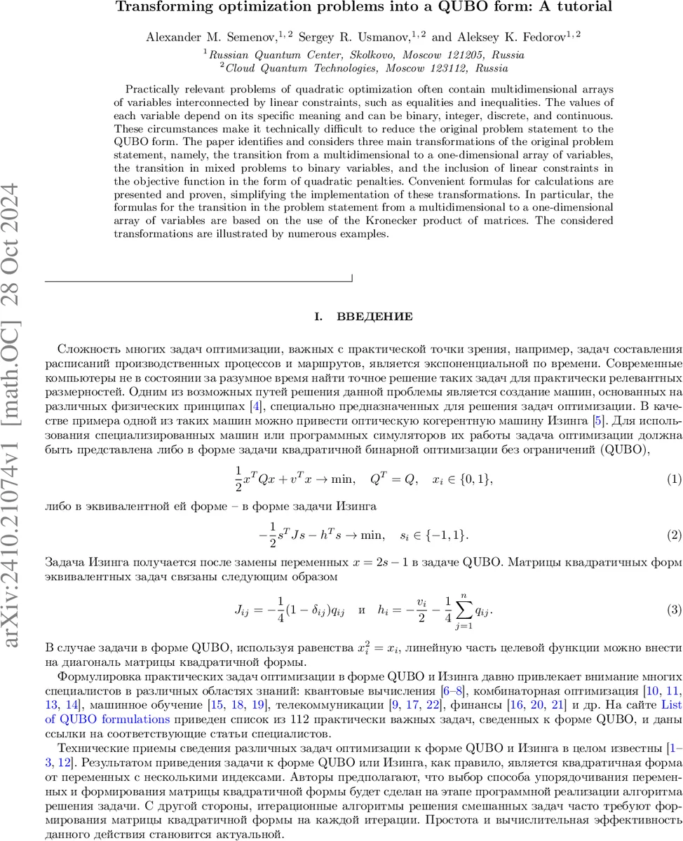
Practically relevant problems of quadratic optimization often contain multidimensional arrays of variables interconnected by linear constraints, such as equalities and inequalities. The values of each variable depend on its specific meaning and can be binary, integer, discrete, and continuous. These circumstances make it technically difficult to reduce the original problem statement to the QUBO form. The paper identifies and considers three main transformations of the original problem statement, namely, the transition from a multidimensional to a one-dimensional array of variables, the transition in mixed problems to binary variables, and the inclusion of linear constraints in the objective function in the form of quadratic penalties. Convenient formulas for calculations are presented and proven, simplifying the implementation of these transformations. In particular, the formulas for the transition in the problem statement from a multidimensional to a one-dimensional array of variables are based on the use of the Kronecker product of matrices. The considered transformations are illustrated by numerous examples.

💡 Research Summary

The manuscript provides a comprehensive tutorial on converting practical quadratic optimization problems—often featuring multidimensional variable arrays and linear equality/inequality constraints—into the standard QUBO (Quadratic Unconstrained Binary Optimization) form required by emerging hardware such as quantum annealers, optical Ising machines, and specialized analog optimizers. The authors identify three essential transformation steps: (1) vectorization of multidimensional variables into a single‑dimensional binary vector, (2) binary encoding (or “binarization”) of integer, discrete, and continuous variables, and (3) incorporation of linear constraints as quadratic penalty terms.

Vectorization
The paper first discusses how to map a tensor‑shaped variable (x_{i_1\ldots i_k}) to a flat vector (\bar x). Two indexing conventions—C‑style (row‑major) and Fortran‑style (column‑major)—are described, with the authors favoring the Fortran ordering for its compatibility with Kronecker‑product algebra. Using the Kronecker product (\otimes), they prove that any quadratic form involving two‑index variables can be written as (\bar x^{T}(B\otimes A)\bar x) (Theorem 1) and that the same construction extends to three or more index dimensions (e.g., (\bar x^{T}(C\otimes B\otimes A)\bar x)). Linear constraints (A\bar x = b) are similarly expressed as ((B\otimes A)\bar x = \bar d) (Theorem 2), and the squared violation (|A\bar x-b|^{2}) expands to a quadratic form involving ((B^{T}B\otimes A^{T}A)). This systematic use of Kronecker products eliminates the need for ad‑hoc index handling and enables straightforward implementation in matrix‑oriented programming environments.

Binary Encoding
The second transformation addresses mixed‑type variables. For each original variable (x_j) with a finite set of admissible values, an affine mapping (x = L y + g) is introduced, where (y) is a binary vector, (L = D_b\otimes a) (with (D_b) a diagonal matrix of scaling factors (b_j) and (a) a row vector of bit‑weights), and (g) a shift vector. Theorem 3 shows that substituting this mapping into the original quadratic objective (\frac12 x^{T}Qx + v^{T}x) yields a new quadratic form in the binary variables: (\frac12 y^{T}(L^{T}QL) y + (L^{T}(Qg+v))^{T} y + f(g)). For integer and discrete variables the binary representation is exact; for continuous variables a prescribed precision (\epsilon) determines the required number of bits, guaranteeing that any feasible continuous value can be approximated within (\epsilon).

Penalty Incorporation
Linear constraints are finally absorbed into the objective via a quadratic penalty (\rho|A x - b|^{2}). Using the vectorized representation from the first step, the penalty contributes an additive term (\rho,\bar x^{T}(A^{T}A)\bar x - 2\rho,b^{T}A\bar x + \rho|b|^{2}). The authors provide sufficient conditions on the penalty coefficient (\rho) (e.g., (\rho) larger than the maximum absolute entry of the original Q matrix) to ensure that any minimizer of the penalized QUBO is also a feasible solution of the original constrained problem.

Illustrative Examples
A series of concrete examples demonstrates the methodology: (i) squaring linear combinations of variables, (ii) summations over one or multiple indices, (iii) cumulative sums using a lower‑triangular matrix, (iv) cyclic sums modeled by a circulant matrix, (v) variable substitution in quadratic forms, and (vi) explicit conversion of Ising spin variables ({-1,1}) to binary ({0,1}). Each example shows how the Kronecker‑product formulas, the affine binary mapping, and the penalty construction combine to produce the final QUBO matrix (Q’) and linear term (v’).

Conclusions
The tutorial establishes a unified, mathematically rigorous pipeline for turning complex, multidimensional, mixed‑type quadratic optimization problems into the QUBO format. By leveraging Kronecker products for vectorization, affine binary encodings for variable discretization, and well‑defined penalty terms for constraints, the approach is both theoretically sound and practically implementable. The authors suggest future work on minimizing the number of binary bits required, automating penalty‑parameter selection, and developing memory‑efficient Kronecker‑product implementations for large‑scale problems. This work thus serves as a valuable reference for researchers and engineers seeking to deploy classical or quantum optimization solvers on real‑world problem instances.