Consensus and Disagreement of Heterogeneous Belief Systems in Influence Networks

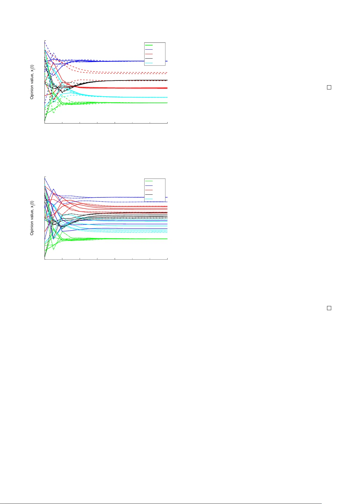
1 Consensus and Disagreement of Heterogeneous Belief Systems in Inﬂuence Networks Mengbin Y e, Member , IEEE Ji Liu, Member , IEEE Lili W ang, Student Member , IEEE Brian D.O. Anderson, Life F ellow , IEEE Ming Cao, Senior Member , IEEE Abstract —Recently , an opinion dynamics model has been proposed to describe a network of individuals discussing a set of logically interdependent topics. For each individual, the set of topics and the logical interdependencies between the topics (captured by a logic matrix) form a belief system. W e inv estigate the role the logic matrix and its structur e plays in determining the ﬁnal opinions, including existence of the limiting opinions, of a strongly connected network of individuals. W e provide a set of results that, given a set of individuals’ belief systems, allow a systematic determination of which topics will reach a consensus, and which topics will disagreement in arise. For irreducible logic matrices, each topic reaches a consensus. For reducible logic matrices, which indicates a cascade interdependence r elationship, conditions are given on whether a topic will reach a consensus or not. It turns out that heter ogeneity among the individuals’ logic matrices, including especially differences in the signs of the off-diagonal entries, can be a key determining factor . This paper thus attributes, for the ﬁrst time, a strong diversity of limiting opinions to heterogeneity of belief systems in inﬂuence networks, in addition to the more typical explanation that strong diversity arises from individual stubbor nness. Index T erms —opinion dynamics, social networks, multi-agent systems, inﬂuence networks, agent-based models, networked systems I . I N T RO D U C T I O N T HERE has been great interest ov er the past few years in agent-based network models of opinion dynamics that describe how indi viduals’ opinions on a topic ev olve ov er time as they interact [1], [2]. The seminal discrete-time French–Harary–DeGroot model [3]–[5] (or DeGroot model for short) assumes that each indi vidual’ s opinion at the next time step is a con vex combination of his/her current opinion and the current opinions of his/her neighbours. This weighted av eraging aims to capture social inﬂuence , where individuals ex ert a conforming inﬂuence on each other so that over time, opinions become more similar (and thus gi ving rise to M. Y e and M. Cao are supported in part by the European Research Council (ERC-CoG-771687) and the Netherlands Organization for Scientiﬁc Research (NWO-vidi-14134). B. D.O. Anderson was supported by the Australian Research Council (ARC) under grant DP-160104500, and by Data61-CSIR O. M. Y e and M. Cao are with the Faculty of Science and Engineering, ENTEG, University of Groningen, Groningen 9747 AG, Netherlands. M. Y e and B.D.O. Anderson are with the Research School of Engineering, Australian National Univ ersity , Canberra, Australia. B.D.O. Anderson is also with Hangzhou Dianzi Univ ersity , China, and with Data61-CSIRO (formerly NICT A Ltd.) in Canberra, Australia. J. Liu is with the Department of Electrical and Computer Engineering, Stony Brook University . L. W ang is with the Department of Electrical Engineering, Y ale University . { m.ye,m.cao } @rug.nl, brian.anderson@anu.edu.au, ji.liu@stonybrook.edu, lili.wang@yale.edu . the term “inﬂuence network”). For networks satisfying mild connectivity conditions, the opinions reach a consensus, i.e. the opinion values are equal for all indi viduals. Since then, and to reﬂect real-world networks, much focus has been placed on developing models of increasing sophis- tication to capture different socio-psychological features that may be in volved when individuals interact. The Hegselmann– Krause model [6]–[9] introduced the concept of bounded conﬁdence, which is used to capture homophily , i.e. the phe- nomenon whereby indi viduals only interact with those other individuals whose opinion values are similar to their own. The Altaﬁni model [10]–[13] introduced negati ve edge weights to model antagonistic or competitiv e interactions between individuals (perhaps arising from mistrust). An individual’ s propensity to assimilate information in a biased manner , by more heavily weighting opinions close to his or her own, is studied in [14]. The Friedkin–Johnsen model generalised the DeGroot model by introducing the idea of “stubbornness”, where an individual remains (at least partially) attached to his or her initial opinion [15], [16]. Of particular note is that the DeGroot and Friedkin–Johnsen models have been empirically examined [16]–[18]. For more detailed discussions on opinion dynamics modelling, we refer the reader to [1], [2], [19]. Recently in [20], a multi-dimensional extension to the Friedkin–Johnsen was proposed to describe a network of individuals who simultaneously discuss a set of logically in- ter dependent topics. That is, an indi vidual’ s position on T opic A may inﬂuence his/her position on T opic B due to his/her view of constraints or relations between the two topics. Such interdependencies are captured in the model by a “logic ma- trix”. This interdependence can greatly shift the ﬁnal opinion values on the set of topics since no w the interdependencies and the social inﬂuence from other individuals both affect opinion values. The model is used in [21] to explain that the shift in the US public’ s opinions on the topic of whether the 2003 In vasion of Iraq was justiﬁed was due to shifting opinions on the logically interdependent topic of whether Iraq had weapons of mass destruction. The set of topics, the interdependent functionalities between the topics, and the mechanism by which an individual processes such interdependencies forms a “belief system” as termed by Con verse in his now classical paper [22]. For networks where all individuals hav e the same logic matrix, a complete stability result is gi ven using algebraic conditions in [20] and using graph-theoretic conditions in [23]. Of course, the assumption that all individuals have the same logic matrix is restrictiv e. Heterogeneous logic matrices were considered in [21], but at least one individual is required to 2 exhibit stubbornness in order to obtain a stability result. This paper will also consider a generalisation of the multi- dimensional model proposed in [20] for the evolution of opin- ions in belief systems, going beyond [20], [21] by analysing the ef fects of the logic matrix, including especially heter ogene- ity of the logic matrices among the individuals, on the limiting opinion distribution . W e ﬁrst establish a general conv ergence result for the model with heterogeneous logic matrices on strongly connected networks. Then, we provide a set of results which enables the systematic determination of whether for a giv en topic, the opinions of the individuals will reach a consensus, or will reach a state of persistent disagreement. W e ﬁnd that the nature of the heterogeneity of the logic structure among the individuals, viz. the logical interdepen- dencies between topics, and the structure itself, plays a major role in determining whether opinions on a giv en topic reach a consensus or fail to do so. If the logical interdependencies do not hav e a cascade structure, then consensus is always secured. When the logical interdependencies have a cascade structure, and by considering topics at the top of a cascade structure to be axiom(s) that an individual’ s belief system is built upon, we establish that discussion of the axiomatic topics will lead to a consensus. In contrast, we discov er that persistent disagreement can arise in the topics at the bottom of the cascade when certain types of heterogeneity exist in the logic matrices. A preliminary work [24] considers the special case of lo wer triangular logic matrices, but we go well beyond that in this paper by considering general logic matrix structures and providing a comprehensiv e account of the results. W e discover that if there is a failure to reach a consensus, then it is typically not minor; in general a str ong diversity of opinions will ev entually emerge. In more detail, a network is said to exhibit weak diversity [25] if opinions eventually con ver ge into clusters where there is no difference between opinions in the same cluster (consensus is the special case of one single cluster). Strong div ersity occurs when the opinions con ver ge to a conﬁguration of persistent disagreement, with a div erse range of v alues (there may be clusters of opin- ions with similar , but not equal , values within a cluster). W eak div ersity is a common outcome in the Hegselmann– Krause model, with the network becoming disconnected into subgroups associated with the clusters. In strongly connected networks, weak di versity also emerges in the Altaﬁni model (speciﬁcally polarisation of two opinion clusters) when the network is “structurally balanced”. Howe ver , sign reversal of some selected edges may destroy the structural balance of the network, causing the opinions to con verge to a consensus at an opinion value of zero, indicating that the polarisation phenomenon is not robust to changes in the network structure. There has been a gro wing interest to study models which are able to capture the more realistic outcome of str ong diversity in networks which remain connected [25], [26]. The DeGroot model shows that social inﬂuence in a connected network acts to bring opinions closer together until a consensus is achiev ed, meaning some other socio-psychological process must be at work to generate strong diversity . The Friedkin– Johnsen model attrib utes strong div ersity to an individual’ s stubborn attachment to his/her initial opinion [15]. In contrast, [27] considers a model where an individual’ s susceptibility to interpersonal inﬂuence is dependent on the individual’ s current opinion; strong div ersity is veriﬁed as a special case. The papers [25], [26] consider two features that might gi ve rise to strong div ersity , the ﬁrst being “social distancing”, and the second being an individual’ s “desire to be unique”. Experimental studies are inconclusive with regards to the existence of ubiquitous and persistent antagonistic interper - sonal interactions (there might be limited occurrences in the network ov er short time spans) [20], while it is unlikely that an individual has the same lev el of stubborn attachment to his or her initial opinion value for months or years. In contrast to these works, we identify for the ﬁrst time in the literature that strong div ersity can arise because of the structure of individuals’ belief systems, and show that heterogeneity among belief systems plays a crucial role. In the model, each individual is concurrently undergoing two driv er processes; individual-le vel belief system dynamics to secure logical consistency of opinions across a set of topics, and interpersonal inﬂuence to reach a consensus. Our ﬁndings explain that when the two drivers do not interfere with each other , a consensus is reached, whereas conﬂict between the two drivers leads to persistent disagreement even though all individuals are trying to reach a consensus. This gi ves a new and illuminating perspectiv e as to why strong diversity can last for extended periods of time in connected networks. The rest of the paper is structured as follows. In Section II, we provide notations, an introduction to graph theory and the opinion dynamics model. At the same time, a formal problem statement is giv en. The main results are presented in Section III, with simulations giv en in Section IV for illustration, and conclusions in Section V. I I . B A C K G RO U N D A N D F O R M A L P RO B L E M S TA T E M E N T W e begin by introducing some mathematical notations used in the paper . The ( i, j ) th entry of a matrix M is denoted m ij . A matrix A is said to be nonnegati ve (respectively positive) if all a ij are nonnegativ e (respecti vely positive). W e denote A as being nonnegati ve and positiv e by A ≥ 0 and A > 0 , respectiv ely . A matrix A ≥ 0 is said to be row-stochastic (respectiv ely , row-substochastic) if there holds P n j =1 a ij = 1 , ∀ i (respectively , if there holds P n j =1 a ij ≤ 1 , ∀ i and ∃ k : P n j =1 a kj < 1 ). The transpose of a matrix M is denoted by M > . Let 1 n and 0 n denote, respectiv ely , the n × 1 column vectors of all ones and all zeros. The n × n identity matrix is giv en by I n . T wo matrices A ∈ R n × m and B ∈ R n × m are said to be of the same type, denoted by A ∼ B , if and only if a ij 6 = 0 ⇔ b ij 6 = 0 . The Kronecker product is denoted by ⊗ . The inﬁnity norm and spectral radius of a square matrix A is k A k ∞ and ρ ( A ) , respectiv ely . A square matrix A ≥ 0 is primitive if ∃ k ∈ N : A k > 0 [28, Deﬁnition 1.12]. A. Graph Theory The interaction between n individuals in a social network, and the logical interdependence between topics can modelled using a weighted directed graph. T o that end, we introduce some notations and concepts for graphs. A directed graph 3 G [ A ] = ( V , E , A ) is a triple where node v i is in the ﬁnite, nonempty set of nodes V = { v 1 , . . . , v n } . The set of ordered edges is E ⊆ V × V . W e denote an ordered edge as e ij = ( v i , v j ) ∈ E , and because the graph is directed, in general the existence of e ij does not imply existence of e j i . An edge e ij is said to be outgoing with respect to v i and incoming with respect to v j . Self-loops are allo wed, i.e. e ii may be in E . The matrix A ∈ R n × n associated with G [ A ] captures the edge weights. More speciﬁcally , a ij 6 = 0 if and only if e j i ∈ E . If A is nonnegati ve, then all edges e ij hav e positiv e weights, while a generic A may be associated with a signed graph G [ A ] , having signed edge weights. A directed path is a sequence of edges of the form ( v p 1 , v p 2 ) , ( v p 2 , v p 3 ) , . . . where v p i ∈ V are unique, and e p i p i +1 ∈ E . Node i is reachable from node j if there exists a directed path from v j to v i . A graph is said to be strongly connected if every node is reachable from e very other node. A square matrix A is irreducible if and only if the associated graph G [ A ] is strongly connected. A directed cycle is a directed path that starts and ends at the same verte x, and contains no repeated vertex except the initial (which is also the ﬁnal) verte x. The length of a directed cycle is the number of edges in the directed cyclic path. A directed graph is aperiodic if there exists no integer k > 1 that divides the length of e very directed cycle of the graph [28]. Note that any graph with a self-loop is aperiodic. A signed graph G is said to be structurally balanced (respec- tiv ely structurally unbalanced) if the nodes V = { v 1 , . . . v n } can be partitioned (respectively cannot be partitioned) into two disjoint sets such that each edge between two nodes in the same set has a positiv e weight, and each edge between nodes in different sets has a negati ve weight [29]. The following is a useful result employed in the paper . Lemma 1 ( [28, Proposition 1.35]) . The graph G [ A ] , with A ≥ 0 , is strongly connected and aperiodic if and only if A is primitive. Note that the irreducibility of A (implied by the strong connectivity property of G [ A ] ) implies that if a k exists such that A k > 0 , then A j > 0 for all j > k . B. The Multi-Dimensional DeGroot Model In this paper , we in vestigate a recently proposed multi- dimensional extension to the DeGroot and Friedkin-Johnsen models [20], [21], which considers the simultaneous discus- sion of logically interdependent topics . Formally , consider a population of n indi viduals discussing simultaneously their opinions on m topics, with indi vidual and topic index set I = { 1 , . . . , n } and J = { 1 , . . . , m } , respectiv ely . Individual i ’ s opinions on the m topics at time t = 0 , 1 , . . . , are denoted by x i ( t ) = [ x 1 i ( t ) , . . . , x m i ( t )] > ∈ R m . In this paper, we adopt a standard deﬁnition of an opinion [21]. In particular , x p i ( t ) ∈ [ − 1 , 1] is individual i ’ s attitude tow ards topic p , which takes the form of a statement, with x p i > 0 representing i ’ s support for statement p , x 1 i < 0 representing rejection of statement p , and x p i = 0 representing a neutral stance. The magnitude of x p i denotes the strength of con viction, with | x p i | = 1 being maximal support/rejection. Mild assumptions are placed on the network and indi vidual parameters in the sequel to ensure that x p i ( t ) ∈ [ − 1 , 1] for all t ≥ 0 , and thus the opinion values are always well deﬁned. In the multi-dimensional DeGroot model, x i ( t ) evolv es according to x i ( t + 1) = n X j =1 w ij C i x j ( t ) , (1) where the nonnegati ve scalar w ij represents the inﬂuence weight individual i accords to the vector of opinions of individual j . Thus, the inﬂuence matrix W , with ( i, j ) th entry w ij , can be used to deﬁne the graph G [ W ] that describes the interpersonal inﬂuences of the n individuals. W e assume that w ii > 0 for all i ∈ I and P n j =1 w ij = 1 for all i ∈ I , which implies that W is ro w-stochastic. The matrix C i , with ( p, q ) th entry c pq ,i , is termed the logic matrix . In [20], [21], the authors elucidate that C i represents the logical interdependence between the m topics as seen by individual i . W e note that the C i are assumed to be heterogeneous (i.e. ∃ i, j : C i 6 = C j ). Indeed, a critical aspect of this paper is to study ho w the structure of the C i s, especially heterogeneity , can determine whether certain topics have opinions that reach a consensus or a persistent disagreement. W e now illustrate with a simple example how C i is used by individual i to obtain a set of opinions consistent with any logical interdependencies between each topic, and in doing so, motiv ate that certain constraints must be imposed on C i due to the problem context (these constraints are implicitly imposed in [20], [21], but without motiv ation). Suppose that there are two topics. T opic 1: The exploration of Space is important to mankind’ s future. T opic 2: The exploration of Space should be pri vatised. Using T opic 1 as an example, and according to the deﬁnition of an opin- ion given abov e Eq. (1), x 1 i = 1 represents indi vidual i ’ s maximal support of the importance of Space exploration, while x 1 i = − 1 represents maximal r ejection that Space exploration is important. Now , suppose that indi vidual i has x i (0) = [1 , − 0 . 2] > , i.e. individual i initially believes with maximal conviction that Space exploration is important and initially believ es with some (but not absolute) conviction that Space exploration should not be privatised 1 . Let C i =  1 0 0 . 5 0 . 5  . (2) This tells us that indi vidual i ’ s opinion on the importance of Space exploration is unaffected by his or her own opinion on whether Space exploration should be priv atised. On the other hand, individual i ’ s opinion on T opic 2 depends positiv ely on his or her o wn opinion on T opic 1 , perhaps because individual i believ es priv atised companies are more effecti ve. In the absence of opinions from other individuals, individual i ’ s opinions ev olves as x i ( t + 1) = C i x i ( t ) , (3) 1 Note that we do not require C i to be row-stochastic and nonnegativ e, though the C i of this example is. 4 which yields lim t →∞ x i ( t ) = [1 , 1] > , i.e. individual i e ventu- ally believ es that Space exploration should be priv atised. Thus, x i ( t ) moves from x i (0) = [1 , − 0 . 2] > , where individual i ’ s opinions are inconsistent with the logical interdependence as captured by C i , to the ﬁnal state x i ( ∞ ) = [1 , 1] > , which is consistent with the logical interdependence. Eq. (3), with opin- ion vector x i ( t ) and the logical interdependencies captured by C i , models individual i ’ s belief system. (W e explained qualitativ ely what a belief system was in the Introduction, and hav e now gi ven the mathematical formulation.) In general, one might expect, as do we in this paper , that an individual’ s belief system without interpersonal inﬂuence from neighbours will ev entually become consistent. For a topic p which is independent of all other topics, one also expects that x p i ( t + 1) = x p i ( t ) for all t . T o ensure the belief system is consistent, we impose the following assumption. Assumption 1. The matrix C i , for all i ∈ I , is such that each eigen value of C i is either 1 or has modulus less than 1. If an eigen value of C i is 1, then it is semi-simple 2 . F or all i ∈ I and p ∈ J , ther e holds P m q =1 | c pq ,i | = 1 , and the diagonal entries satisfy c pp,i > 0 . The assumptions on the eigen values of C i ensure that Eq. (3) con verges to a limit, and are necessary and sufﬁcient for individual i ’ s belief system to eventually become consis- tent. The other assumptions lead to desirable properties for the system Eq. (1). Speciﬁcally , the reasonable assumption that c pp,i > 0 means topic p is positiv ely correlated with itself. The constraint P m q =1 | c pq ,i | = 1 for all i ∈ I and p ∈ J ensures that x p i (0) ∈ [ − 1 , 1] implies x p i ( t ) ∈ [ − 1 , 1] for all t ≥ 0 (see [20]), and also implies that if topic p is independent of all other topics, i.e. c pq ,i = 0 for all q 6 = p , then c pp,i = 1 . The well-studied special case where topics are totally independent is C i = I m . W e are now in a position to formally deﬁne this paper’ s objectiv e. C. Objective Statement This paper is focused on establishing the effects of the set of logic matrices C i , i ∈ I on the ev olution of opinions, and in particular the limiting opinion conﬁguration. First, we record two assumptions on the logic matrix and the network topology , which will hold throughout this paper . Assumption 2. F or every i, j ∈ I , there holds C i ∼ C j . Assumption 3. The inﬂuence network G [ W ] is str ongly con- nected, W is r ow-stochastic, and w ii > 0 , ∀ i ∈ I . Assumption 2 implies that, for ev ery i, j ∈ I , the graphs G [ C i ] and G [ C j ] hav e the same structure (but possible with different edge weights, including weights of opposing signs). This means that all individuals have the same view on which topics have dependent relationships with which other topics, but the assigned weights c ij (and signs) may be different. This assumption ensures that the scope of this paper is reasonable, because otherwise the assumption that C i ∼ C j does not hold would introduce too many different scenarios to analyse. 2 By semi-simple, we mean that the geometric and algebraic multiplicities are the same. Equiv alently , all Jordan blocks of the eigen value 1 are 1 by 1. Objective 1. Let a set of logic matrices C i , i ∈ I and an inﬂuence network G [ W ] be given, satisfying Assumptions 1, 2 and 3. Suppose that each individual i ’s opinion vector x i ( t ) ∈ [ − 1 , 1] m evolves accor ding to Eq. (1). Then, for each k ∈ J and generic initial conditions x (0) ∈ [ − 1 , 1] nm , this paper will in vestigate a method to systematically determine when ther e e xists, and when ther e does not exist, an α k ∈ [ − 1 , 1] such that lim t →∞ x k i ( t ) = α k , ∀ i ∈ I . (4) W e will show that C i of a certain structure always guar- antees consensus, and conv ersely , that C i of a certain other structure will lead to disagreement in certain identiﬁable topics. Next, we provide further discussion to motiv ate Objective 1, including our interest in heterogeneous C i . The dynamics of the form Eq. (1) is a variation on the model studied in [20], [21], and we explain our interest in this particular variation by explaining in detail the differences between Eq. (1) and work in [20], [21]. For con venience, denote the vector of opinions for the entire inﬂuence network as x = [ x 1 ( t ) > , . . . , x n ( t ) > ] > ∈ R nm . Supposing that the logic matrices were indeed homogeneous, i.e. C i = C j = C for all i, j ∈ I , we can verify that much of the analysis becomes rather easy . For then one could write the inﬂuence network dynamics as x ( t + 1) = ( W ⊗ C ) x ( t ) , (5) and limiting behaviour is characterised by the following result. Theorem 1 ( [20, Theorem 3]) . The system Eq. (5) con- ver ges if and only if lim k →∞ C k , C ∞ exist, and either C ∞ = 0 m × m or lim k →∞ W k = W ∞ exists 3 . Mor eover , the system con ver ges to lim t →∞ x ( t ) = ( W ∞ ⊗ C ∞ ) x (0) if lim k →∞ W k = W ∞ exists, otherwise lim t →∞ x ( t ) = 0 mn . For completeness and to aid discussion, we also record the Friedkin–Johnsen variant to Eq. (1), which is gi ven as x i ( t + 1) = λ i n X j =1 w ij C i x j ( t ) + (1 − λ i ) x i (0) . (6) Here, the parameter λ i ∈ [0 , 1] represents individual i ’ s susceptibility to interpersonal inﬂuence, while 1 − λ i represents the lev el of stubborn attachment by indi vidual i to his/her initial opinion x i (0) . This paper studies the special case where there are no stubborn indi viduals, i.e. λ i = 1 for all i ∈ I , and thus Eq. (6) is equiv alent to Eq. (1). The paper [20] mainly focuses on the considerable challenge of obtaining complete con vergence results for the model in Eq. (6) but with a homogeneous C , and aside from some short remarks, does not in vestigate the effect of C on the ﬁnal opinion distribution (assuming the opinions do in fact con ver ge to a steady state). The paper [21] secures a con vergence result for heterogeneous C i but makes an assumption that there is at least one some what stubborn individual. Unlike [20] and [21], the key focus of this paper is to in vestigate the effect of the 3 It is clear that if we hav e homogeneous C , then Assumption 1 is consistent with the requirement on C in Theorem 1. 5 structur e of C i , including heter ogeneity , on the ﬁnal opinion distribution. W e explain this further . If λ i < 1 and C i = I m for all i ∈ I , then existing results establish that under Assumption 3, a strong di versity of opinions emerges [20], with obviously no effects arising from the C i matrix. On the other hand, consider the case of homogeneous logic matrices and no stubbornness. For any W satisfying Assumption 3, it is known that lim k →∞ W k = 1 n γ > where γ > is a left eigenv ector of W associated with the simple eigenv alue at 1 , having entries γ j > 0 , and normalised to satisfy γ > 1 n = 1 [28]. Combining with Theorem 1, we can conclude that under Assumption 3 and if C i = C j = C and λ i = 1 for all i, j ∈ I , the opinions of all indi viduals on any given topic reach a consensus. That is, for all i ∈ I , there holds lim t →∞ x i ( t ) = P n j =1 γ j C t x j (0) . In contrast, this paper assumes heterogeneous C i and no stubbornness among individuals. If we can sho w that opinions on a giv en topic fail to reach a consensus in the general case of C i 6 = I m , and instead strong div ersity emerges, then this failure must be attributed to the structure, and the heter o- geneity , of the C i among individuals. This would constitute a nov el insight into the emergence of strong div ersity in strongly connected networks, linking it for the ﬁrst time to differences in individuals’ belief systems as opposed to stubbornness [15], a desire to be unique [25], [26], or social distancing [25]. T o conclude this subsection, we now provide the deﬁnition of “competing logical interdependencies” which will be impor- tant in some scenarios for characterising the ﬁnal opinions. Deﬁnition 1 (Competing Logical Interdependence) . An inﬂu- ence network is said to contain individuals with competing logical inter dependencies on topic p ∈ J if there e xist individuals i, j such that for some q ∈ J \ { p } , C i and C j have nonzero entries c pq ,i and c pq ,j that are of opposite signs. In other words, individuals with competing logical interde- pendencies are those who, when having the same opinion on topic q , move in opposite directions on the opinion spectrum for topic p . Such occurrences can be prev alent in society . Using the example in Section II-B, one might hav e an individual j with C j =  1 0 − 0 . 5 0 . 5  . (7) because j considers that priv ate companies are proﬁt-dri ven, and therefore cannot be ethically trusted with the exploration of Space. Then, from Eq. (3), one has that x j ( ∞ ) = [1 , − 1] > , i.e. individual j ev entually ﬁrmly belie ves Space exploration should not be priv atised. In particular , x 1 j ( ∞ ) = − x 2 j ( ∞ ) . In light of Assumption 2, if two individuals have competing interdependencies on topic p , then for every individual i ∈ I , there is necessarily some individual k ∈ I \ { i } with whom individual i has competing logical interdependence on topic p : the nonzero entries c pq ,i and c pq ,k are of opposite signs for some q ∈ J . Remark 1. Recall that C i is individual i ’ s set of con- straints/functional dependencies between topics in i ’s belief system. Thus, heter ogeneity of C i may arise for many differ ent r easons, such as education, backgr ound, or expertise in the topic. F or example, if the set of topics is r elated to sports, a pr ofessional athlete may have very differ ent weights in C i compar ed to someone that does not pur sue an active lifestyle. Competing interdependencies may also arise for contentious issues, such as gun contr ol discussions in the USA. Inter estingly , [30] showed that when pr esented with the same published statement on an issue, differ ent people could take opposite positions on the issue. In the next section, we provide the set of main theoretical results of this paper to address Objectiv e 1. I I I . M A I N R E S U L T S The main results are presented in two parts. First, we es- tablish a general con vergence result for the networked system. Then, we analyse the limiting opinion distribution and the role of the set of logic matrices in determining whether opinions for a giv en topic reach consensus or fail to do so. In order to place the focus on the theoretical results and interpretations as social phenomena, all proofs are presented to the Appendix. A. Con verg ence The network dynamics of Eq. (1) are giv en by x ( t + 1) =    w 11 C 1 · · · w 1 n C 1 . . . . . . . . . w n 1 C n · · · w nn C n    x ( t ) , (8) and we deﬁne the system matrix abo ve as B . T o begin, we re write the network dynamics Eq. (8) into a differ - ent form to aid analysis by introducing a coordinate trans- form (actually a reordering). In particular, deﬁne y k ( t ) = [ y 1 k ( t ) , . . . y n k ( t )] > = [ x k 1 ( t ) , . . . , x k n ( t )] > , for k ∈ J as the vector of all n individuals’ opinions on the k th topic. Then, y ( t ) = [ y 1 ( t ) > , . . . , y m ( t ) > ] > captures all of the n individuals’ opinions on the m topics. One obtains that y k ( t + 1) = m X j =1 diag ( c kj ) W y j ( t ) , (9) where diag ( c kj ) ∈ R n is a diagonal matrix with the i th diagonal element of diag ( c kj ) being c kj,i , the ( k , j ) th entry of C i . It follows that y ( t + 1) =    diag ( c 11 ) W · · · diag ( c 1 m ) W . . . . . . . . . diag ( c m 1 ) W · · · diag ( c mm ) W    y ( t ) . (10) W e denote the matrix in Eq. (10) as A , with block matrix elements A pq = diag ( c pq ) W . W e now show how the system Eq. (10) can be considered as a consensus process on a multiplex (or multi-layered) signed graph. Consider the matrix A in Eq. (10), with the associated graph G [ A ] , and the matrix B in Eq. (8), with associated graph G [ B ] . Clearly , the two graphs are the same up to a reordering of the nodes. In G [ A ] , with node set V [ A ] = { v 1 , . . . , v nm } , one can consider the node subset V p = { v ( p − 1) n +1 , . . . , v pn } , p ∈ J as a layer of the multi-layer graph G [ A ] with vertices associated with the opinions of individuals 1 , . . . , n on topic 6 x 1 1 x 2 1 x 3 1 x 1 2 x 2 2 x 3 2 w ij y 1 1 y 1 2 y 1 3 y 2 1 y 2 2 y 2 3 w ij G [ B ] G [ A ] ⇔ ˜ V 1 ˜ V 2 V 2 V 1 V 3 Figure 1. An illustrative network with 2 individuals discussing 3 topics, with only selected edges drawn for clarity . Each node represents the opinion of an individual for a topic, with red and blue nodes associated with individuals 1 and 2, respectively . The black edges represent interpersonal inﬂuence via the weight w ij , while the coloured edges represent logical interdependencies between topics. In G [ B ] , nodes are grouped and ordered by individual in node subset ˜ V q (as illustrated by the dotted green ellipse groupings) leading to Eq. (8). In G [ A ] , the nodes are grouped and ordered by topic in node subset V p (as illustrated by the dotted green ellipses) leading to Eq. (10). p . In G [ B ] , with node set V [ B ] = { v 1 , . . . , v nm } , one can consider the node subset ˜ V q = { v ( q − 1) m +1 , . . . , v q m } , q ∈ I as a layer of a multi-layer graph with vertices associated with the opinions of individual q on topics 1 , . . . , m . This is illustrated in Fig. 1, where each layer is identiﬁed by a dotted green ellipse border . A key moti vation to study G [ A ] and the dynamical system Eq. (10) is that all the block diagonal entries A ii of A are nonnegati ve and irreducible because Assumption 1 indicates that diag ( c pp ) has positive diagonal entries. This means that the edges between nodes in the subset V p = { v ( p − 1) n +1 , . . . , v pn } , p ∈ J have positiv e weights, and this property greatly aids in the checking of the structural balance or unbalance of the network G [ A ] giv en G [ W ] and C i , ∀ i ∈ I . V erify from the row-stochastic property of W and the row- sum property of C i in Assumption 1 that the entries of A satisfy P nm q =1 | a pq | = 1 for all p = 1 , . . . , nm . W e therefore conclude that Eq. (10) has the same dynamics as the discrete- time Altaﬁni model (see e.g. [10], [11]). Remark 2. Although Eq. (10) has the same dynamics as the discr ete-time Altaﬁni model, a number of important differ ences exist. F irst, the context of ne gative edge weights is entir ely differ ent: in the Altaﬁni model, w ij < 0 implies individual i mistrusts individual j [10]. In contrast, Eq. (10) assumes nonne gative inﬂuence w ij ≥ 0 , and the ne gative edge weights arise fr om negative logical inter dependencies in C i . Moreo ver the network structur e of G [ A ] is affected by both the inﬂuence network G [ W ] and the logic matrix graphs G [ C i ] . The main con vergence result is giv en as follows. Theorem 2. Suppose that for a population of n individuals, the vector of the n individuals’ opinions y ( t ) evolves ac- cor ding to Eq. (10), with interpersonal inﬂuences captur ed by G [ W ] . Suppose further that Assumptions 1, 2, and 3 hold. Then, for any initial condition y (0) ∈ R nm , ther e exists some y ∗ ∈ R nm such that ther e holds lim t →∞ y ( t ) = y ∗ exponentially fast. If y i k (0) ∈ [ − 1 , 1] for all i ∈ I and k ∈ J , then y i k ( t ) ∈ [ − 1 , 1] for all t ≥ 0 and i ∈ I and k ∈ J . Having established that the opinion dynamical system al- ways con ver ges, we now address Objectiv e 1 by studying the inﬂuence of C i in determining the limiting opinion vector y ∗ . B. Consensus and Disagr eement of Each T opic W e no w explain ho w to use the logic matrices C i to systematically determine whether opinions on a given topic p ∈ J will reach a consensus or not. W e defer discussion of the social interpretation of the theoretical results until Section III-C, and illustrate some of the conclusions drawn in this section with selected simulations in Section IV. Consider the graph G [ C i ] associated with C i for some i ∈ I , which is a signed graph if there are negati ve off- diagonal entries in C i . It turns out (see Theorem 3 imme- diately below) that if C i for all i ∈ I are irreducible, then all topics will reach a consensus (although the consensus value for two dif ferent topics p and q may be dif ferent). W e remark that irreducible logic matrices correspond to G [ C i ] which are strongly connected, and thus for any two topics p, q ∈ J , there is a (possibly signed) directed path from p to q . In other words, all topics are directly or indirectly dependent on all other topics. Theorem 3. Let the hypotheses in Theor em 2 hold. Suppose that (i) y i k (0) ∈ [ − 1 , 1] for all i ∈ I and k ∈ J , and (ii) that Assumptions 1, 2, and 3 hold. Suppose further that C i , ∀ i ∈ I ar e irr educible 4 . Then, for all k ∈ J , lim t →∞ y k ( t ) = α k 1 n exponentially fast, where α k ∈ [ − 1 , 1] . Mor eover , 1) If there are no competing logical inter dependencies, as given in Deﬁnition 1, and G [ C i ] , ∀ i ∈ I ar e structurally balanced 5 , then for almost all initial conditions, | α p | = | α q | 6 = 0 , ∀ p, q ∈ J . 2) If there are no competing logical inter dependencies, and G [ C i ] , ∀ i ∈ I are structurally unbalanced, then α k = 0 , ∀ k ∈ J . 3) If there ar e competing logical interdependencies, then α k = 0 , ∀ k ∈ J . Further to the conclusions of Theorem 3, one can obtain the following result for the case where consensus to a nonzero opinion value is achiev ed. Corollary 1. Let the hypotheses in Theorem 3 hold. Suppose that ther e ar e no competing logical inter dependencies, and G [ C i ] , ∀ i ∈ I ar e structurally balanced. F or G [ C i ] with node set V = { v 1 , . . . , v m } , deﬁne two disjoint subsets of nodes V [ C i ] + and V [ C i ] − so that each edge between two nodes in V [ C i ] + or two nodes in V [ C i ] − has a positive weight, and each edge between two nodes in V [ C i ] + and V [ C i ] − has a ne gative weight. Then, for any p, q ∈ J , there holds 1) α p = α q if v q , v p ∈ V [ C i ] + or v q , v p ∈ V [ C i ] − . 2) α p = − α q if v q ∈ V [ C i ] + and v p ∈ V [ C i ] − . Consider no w the more general case where C i for all i ∈ I are reducible. Thus, G [ C i ] is no longer strongly connected. 4 Under Assumption 2, irreducibility of one C i implies the same for all. 5 Under Assumption 2 and in the absence of competing logical interdepen- dencies, the presence or absence of structural balance for one C i implies the same for all. 7 The logic matrices of all indi viduals can be expressed in a lower block triangular form through an inessential reordering of the topic set. From Assumption 2, we further conclude that there exists a common permutation matrix P such that, for all i ∈ I , P T C i P is lower block triangular . Without loss of generality , we therefore assume that the topics p ∈ J are ordered such that, for each i ∈ I , C i =      C 11 ,i 0 · · · 0 C 21 ,i C 22 ,i · · · 0 . . . . . . . . . . . . C s 1 ,i C s 2 ,i · · · C ss,i      , (11) where C j j,i ∈ R s j × s j is irreducible for any j ∈ S , { 1 , 2 , · · · , s } and s j are positive integers such that P s j =1 s j = m . Decompose the opinion set J into s disjoint subsets J j for j ∈ S where J j , { j X i =1 s i − 1 + 1 , j X i =1 s i − 1 + 2 , . . . , j X i =1 s i − 1 + s j } , (12) with s 0 = 0 . Though reducible C i may seem to be restrictive, they are in fact common giv en the problem context since they imply a cascade logical interdependence structure among the topics. This may be representati ve of an indi vidual i who obtains C i by sequentially building upon an axiom or axioms (the ﬁrst C j j,i block matrices). The two topics of the Space exploration e xample given in Eq. (2) constitute one such example of a belief system driven by an axiom (T opic 1). From the perspectiv e of the graph G [ C i ] , the expression in Eq. (11) enables G [ C i ] to be divided into strongly connected components which are “closed” or “open”. (This is related to a concept called the condensation of a graph, see [28]). Formally , we say that a subgraph ¯ G is a strongly connected component of G if ¯ G is strongly connected and any other subgraph of G strictly containing ¯ G is not strongly connected. A strongly connected component ¯ G of a graph G is said to be closed if there are no incoming edges to ¯ G from a node outside of ¯ G , and is said to be open otherwise. The simplest possible strongly connected component is a single node, and it would be closed if there were no incoming edges to it. Figure 2 shows an example of a graph G [ C i ] divided into strongly connected components (identiﬁed by the dotted line encircling a set of nodes), with the blue and purple components being closed, and the green and orange components being open. Following the notation in Eq. (11) and Eq. (12), we have for the example in Fig. 2, s = 4 , s 1 = 3 , s 2 = 1 , s 3 = 2 , s 4 = 1 , and J 1 = { 1 , 2 , 3 } , J 2 = { 4 } , J 3 = { 5 , 6 } , J 4 = { 7 } . If the topic set J j corresponds to a closed strongly connected component of G [ C i ] , then clearly in Eq. (11), C pj,i = 0 for all p 6 = j . One can then use Theorem 3 and Corollary 1 to establish that for ev ery k ∈ J j , there holds lim t →∞ y k ( t ) = α k 1 n exponentially fast, with α k ∈ [ − 1 , 1] . That is, all opinions in topic k ∈ J j reach a consensus. If, on the other hand, the topic set J j corresponds to an open strongly connected component of G [ C i ] , then the results presented below can be employed sequentially in order to establish whether opinions on a gi ven topic hav e reached a consensus. By “sequentially”, we mean that we analyse G [ C i ] 1 2 3 4 5 6 7 Figure 2. An illustrativ e example of G [ C i ] , with each node representing a topic, and edges representing logical interdependencies between topics (self- loops are hidden for clarity). One can divide the nodes into strongly connected components (each dotted coloured circle denotes a strongly connected com- ponent). The results of this paper allow one to progressively analyse each component to establish which topics will hav e opinions reaching a consensus and which topics will have opinions reaching a persistent disagreement. the topic sets J j with j in the order 1 , 2 , . . . , s . Under Assumption 2, deﬁne for each topic p ∈ J , the set ˆ J p , { q ∈ J : c pq ,i 6 = 0 , q 6 = p } (13) where c pq ,i is the pq th entry of C i . In other words, ˆ J p identiﬁes all topics q ∈ J that topic p is logically dependent upon. Because of Assumption 2, the set ˆ J p is the same for all individuals i ∈ I . In Fig. 2, ˆ J 6 for example is { 4 , 5 } . W e present necessary and sufﬁcient conditions that ensure ev ery topic in the subset J j reaches a consensus of opinions in two theorems, the ﬁrst for the case when the subset J j is a singleton (e.g. J 4 = { 7 } in Fig. 2), and the second for when J j has at least two elements (e.g. J 3 = { 5 , 6 } in Fig. 2). Theorem 4. Let the hypotheses in Theor em 2 hold. Assume that (i) y i k (0) ∈ [ − 1 , 1] for all i ∈ I and k ∈ J , and (ii) that C i , ∀ i ∈ I is decomposed as in Eq. (11). Suppose that J j = { p } , as deﬁned in Eq. (12), is a singleton, and let ˆ J p as deﬁned in Eq. (13) be nonempty . Suppose further that all topics q ∈ ˆ J p satisfy lim t →∞ y q = α q 1 n , α q ∈ [ − 1 , 1] . Then, lim t →∞ y p ( t ) = α p 1 n for some α p ∈ R if and only if there exists a κ ∈ [ − 1 , 1] such that κ = P q ∈ ˆ J p α q c pq ,i P q ∈ ˆ J p | c pq ,i | , ∀ i ∈ I . (14) If such a κ exists, then α p = κ . The key necessary and sufﬁcient condition inv olves Eq. (14), which is somewhat complex and nonintuitiv e. W e now provide a corollary which studies the condition in Eq. (14) for some situations which are important or of interest in the social context. Discussion and interpretation of these formal results are provided in the following Section III-C. Corollary 2. Adopting the hypotheses in Theorem 4, the following hold: 1) Suppose that ˆ J p = { q } is a singleton. Then, ther e exists a κ ∈ [ − 1 , 1] satisfying Eq. (14) if and only if ther e 8 do not exist individuals i, j ∈ I with competing logical inter dependencies on topic p (as deﬁned in Deﬁnition 1). 2) If α q = 0 for all q ∈ ˆ J p , then κ = 0 satisﬁes Eq. (14). 3) Suppose that ˆ J p = { q 1 , . . . , q r } , r ≥ 2 . If c pq k ,i = c pq k ,j = c pq k for all k ∈ { 1 , . . . , r } and i, j ∈ I , then ther e exists a κ ∈ [ − 1 , 1] satisfying Eq. (14). 4) Suppose that ˆ J p = { q 1 , . . . , q r } , r ≥ 2 . Suppose further that | α q u | = | α q v | for all u, v ∈ { 1 , . . . , r } . Then, ther e exists a κ ∈ [ − 1 , 1] satisfying Eq. (14) if either (i) the sign of c pq k ,i and α q k ar e equal for all i ∈ I and k ∈ { 1 , . . . , r } or (ii) the sign of c pq k ,i and α q k ar e opposite for all i ∈ I and k ∈ { 1 , . . . , r } . In the case of (i), κ = | α q k | , and in the case of (ii), κ = −| α q k | . When J j is not a singleton, the analysis becomes signif- icantly more in volv ed. T o that end, we ﬁrst introduce some additional notation. Deﬁne ˜ J j , ∪ k ∈J j ˆ J k \ J j (15) as the set of topics not in J j that the topics in J j depend upon. For example, in Fig. 2, J 3 = { 5 , 6 } , ˆ J 5 = { 3 , 6 } , ˆ J 6 = { 4 , 5 } , and ˜ J 3 = { 3 , 4 } . Note that if J j = { p } is a singleton, we hav e ˜ J j = ˆ J p . Perhaps unsurprisingly , Theorem 4 requires that consensus must ﬁrst occur for topics in ˜ J j = ˆ J p , on which the topics in J j depend. The following theorem also has the requirement that consensus occur for all topics in ˜ J j . Theorem 5. Let the hypotheses in Theor em 2 hold. Assume that (i) y i k (0) ∈ [ − 1 , 1] for all i ∈ I and k ∈ J , and that (ii) C i , ∀ i ∈ I is decomposed as in Eq. (11). Suppose that J j , as deﬁned in Eq. (12), has at least two elements. Let ˜ J j , as deﬁned in Eq. (15), be nonempty and suppose further that all topics q ∈ ˜ J j satisfy y ∗ q = α q 1 n , α q ∈ [ − 1 , 1] . Then, lim t →∞ y k = α k 1 n for all k ∈ J j if and only if, for every k ∈ J j , there exists a φ k ∈ [ − 1 , 1] such that φ k   X r ∈J j \{ k } | c kr,i | + X q ∈ ˜ J j | c kq ,i |   = X r ∈J j \{ k } φ r c kr,i + X q ∈ ˜ J j α q c kq ,i , ∀ i ∈ I (16) If such a set of φ k exist, then α k = φ k for all k ∈ J j . Similar to above, we now present a corollary which gives sufﬁcient conditions for Eq. (16) in two scenarios. Corollary 3. Adopting the hypotheses in Theorem 5, the following hold: 1) If α q = 0 for all q ∈ ˜ J j , then φ k = 0 ∀ k ∈ J j satisﬁes Eq. (16). 2) If c kp,i = c kp,h for all k ∈ J j , p ∈ J and i, h ∈ I , then ther e exist φ k ∈ [ − 1 , 1] satisfying Eq. (16) ∀ k ∈ J j . For the illustrativ e example in Fig. 2, one w ould ﬁrst analyse the blue and purple components using Theorem 3. Then, one would analyse the green component using Theorem 5, and last the orange component using Theorem 4. C. Discussion and Social Interpretations W e conclude this section by providing some discussion and comments on the main results, focusing in particular on the theorems and corollaries in Section III-B. Overall, the outcomes we have established depend on the graphical structures G [ C i ] on the one hand, and on the numerical values (including their signs) of the C i entries on the other . This dependence sometimes ﬂows simply from the signs (the presence or absence of competing logical interdependencies), and sometimes from the precise values of the C i . Further, when consensus on a topic occurs, it is evident that sometimes a value 0 is alw ays the outcome, and sometimes a nonzero value dependent on the initial opinions of those topics in the closed and strongly connected components of G [ C i ] . It is clear from Theorem 3 that for any topic set J j corresponding to a closed and strongly connected component of G [ C i ] , ev ery topic k ∈ J j will reach a consensus. One interpretation is that a closed and strongly connected com- ponent corresponds to J j having a topic(s) that is an axiom (or axioms) upon which an individual builds his or her belief system (see below Eq. (12)). Our results show that discussion of axiomatic topics will alw ays lead a consensus under the model Eq. (1) (a consensus might not be reached if, as in Eq. (6), there is stubbornness present). Theorem 3 and Corollaries 2 and 3 also illustrate that competing logical inter dependencies , if present, can play a major role in determining the ﬁnal opinion values. For in- stance, see Theorem 3 Part 3, where given a topic set J j corresponding to a closed and strongly connected component of G [ C i ] , all opinion values for all topics in J j con ver ge to the neutral value at 0 whenev er competing interdependencies are present in the topics in J j . Also, the presence of any competing logical interdependencies in topic p ∈ J j is enough to prev ent the sufﬁcient conditions detailed in Corollary 2 Item 1), 3), and 4) and Corollary 3 Item 2) from being satisﬁed. Of particular note is Corollary 2 Item 1). When ˆ J p = { q } is a singleton, heterogeneity in the entries of c pq ,i is not enough to prev ent a consensus of opinions on topic p ; competing logical interdependences are required. This last ﬁnding is a surprising, and non-intuitive result. The sufﬁcient condition in Corollary 2 Item 2) requires α q = 0 for all q ∈ ˆ J p . This is not as restricti ve as it ﬁrst seems: one possible scenario is that all elements of ˆ J p belong to topics from the same closed and strongly connected component in G [ C i ] , with the component being structurally unbalanced, or having competing logical interdependencies. The same can be said for Corollary 3 Item 1). Part of the sufﬁcient condition for Corollary 2 Item 4) is that | α q u | = | α q v | for all q u , q v ∈ ˆ J p = { q 1 , . . . , q r } , r ≥ 2 . This will always hold if q 1 , . . . , q r are topics that are part of the same closed and strongly connected component in G [ C i ] . From numerous simulations, we frequently observed that minor heterogenieties in the entries of c pq ,i , p ∈ J j among the individuals (e.g. if the c pq ,i were all selected from a uni- form distribution) were often sufﬁcient to create disagreement among the opinions on topic p ∈ J j . W e observed this in many different examples, except in the case of Corollary 2 Item 1), 9 where J j = { p } and ˆ J p = { q } are both singletons, since existence of competing logical interdependencies was prov en to be a necessary and sufﬁcient condition for disagreement. It is also clear from Theorems 3, 4 and 5 that disagreement is possible only in topic sets J j associated with an open strongly connected component of G [ C i ] . Put another way , belief systems with a cascade logical structure, viz. reducible C i in the form of Eq. (11), including heterogeneity among individuals’ belief systems, play a signiﬁcant role in gen- erating disagreement when social networks discuss multiple logically interdependent topics. Looking at Eq. (1), one can see two separate processes occurring: the DeGroot component describes interpersonal inﬂuence between individuals in an effort to reach a consensus, while the logic matrix by itself (as in Eq. (3)) captures an intrapersonal effort to secure logical consistency of opinions across se veral topics. These two drivers may or may not end up in conﬂict, and the presence of conﬂict or lack thereof determines whether opinions of a certain topic reach a consensus or fail to do so. Our results in Theorems 4 and 5 identify when such conﬂict can occur . Remark 3. Theorems 4 and 5 establish necessary and sufﬁ- cient conditions for topic p k ∈ J j = { p 1 , . . . , p s j } to r each a consensus under a particular hypothesis. Speciﬁcally , it is assumed that for the set J j under consideration, there holds y ∗ q = α q 1 n , ∀ q ∈ ˜ J j . (17) That is, all other topics that one or more topics p k ∈ J j de- pend upon ar e assumed to have reac hed a consensus. Based on numer ous simulations, we believe the requir ement that Eq. (17) holds is also a necessary condition for y p k , p k ∈ J j to reac h a consensus. In other words, if any topic q ∈ ˜ J j fails to r each a consensus, we conjectur e that all y p k , k = 1 , . . . , s j will also fail to reac h a consensus. Conﬁrming this would pro vide yet another indication that networks with belief systems having a cascade logic structur e more r eadily result in disagr eement. W e leave this to future in vestigations. I V . S I M U L A T I O N S W e now provide simulations to illustrate some of the results in Section III using a netw ork G [ W ] of n = 6 individuals, with W =         0 . 2 0 0 0 0 . 8 0 0 . 5 0 . 3 0 0 0 0 . 2 0 0 . 3 0 . 1 0 0 0 . 6 0 0 0 . 85 0 . 15 0 0 0 0 0 0 . 2 0 . 8 0 0 0 0 0 0 . 5 0 . 5         . (18) Note that W satisﬁes Assumption 3. Initial conditions are generated by selecting each x p i (0) from a uniform distribution in [ − 1 , 1] , and the same initial conditon vector x (0) is used for all simulations. W e consider 5 topics, i.e. J = { 1 , . . . , 5 } . In the ﬁrst simulation, we use two logic matrices: b C =       1 0 0 0 0 − 0 . 5 0 . 5 0 0 0 − 0 . 3 − 0 . 6 0 . 1 0 0 0 − 0 . 3 0 0 . 2 − 0 . 5 0 − 0 . 5 0 − 0 . 2 0 . 3       (19a) ¯ C =       1 0 0 0 0 − 0 . 8 0 . 2 0 0 0 − 0 . 3 − 0 . 1 0 . 6 0 0 0 − 0 . 3 0 0 . 2 − 0 . 5 0 − 0 . 5 0 − 0 . 2 0 . 3       . (19b) The individuals hav e logic matrix C i = b C for i = 1 , 2 , 3 and C i = ¯ C for i = 4 , 5 , 6 . Notice that there are no competing logical interdependencies associated with the set of C i . Moreov er, according to Eq. (12), we ha ve J 1 = { 1 } , J 2 = { 2 } , J 3 = { 3 } , J 4 = { 4 , 5 } . The temporal e volution of x ( t ) is giv en in Fig. 3, where solid or dotted lines correspond to an individual with C i = b C or C i = ¯ C , respectiv ely . W e see that T opic 1 (Theorem 3) and T opic 2 (Corollary 2, Statement 1) ) reach a consensus. In particular , notice that the entries of b C and ¯ C are such that b c 21 6 = ¯ c 21 but T opic 2 still reaches a consensus because there are no competing logical interdependencies in T opic 2. In contrast, T opic 3 fails to reach a consensus (Theorem 4) despite both T opics 1 and 2 reaching a consensus. Strong diversity emerges because the heterogeneities in the third row of b C and ¯ C are such that there does not exist a κ ∈ [ − 1 , 1] that satisﬁes Eq. (14), ev en though the sign patterns in the third ro w are the same between b C and ¯ C . T opics 4 and 5, forming J 4 , both reach a consensus because the fourth and ﬁfth rows of b C and ¯ C are the same (Corollary 3, Statement 2) ). Replacing b C with e C =       1 0 0 0 0 0 . 5 0 . 5 0 0 0 − 0 . 3 − 0 . 1 0 . 6 0 0 0 − 0 . 3 0 0 . 2 − 0 . 5 0 − 0 . 5 0 − 0 . 2 0 . 3       (20) for individuals 1 , 2 , 3 , we run the same simulation (i.e. with the same G [ W ] and initial conditions x (0) ). The results are displayed in Fig. 4. Notice that the only difference between b C and e C is a sign rev ersal in the c 21 entry . Now , there are competing logical interdependencies in T opic 2, which results in a failure to reach consensus on this topic (Corollary 2, Statement 1) ). Because of the cascade logic structure, T opics 3, 4 and 5 also fail to reach a consensus (illustrating our conjecture in Remark 3). This is despite no other differences when comparing b C and e C , and T opics 4 and 5 reaching a consensus in the previous simulation when individuals 1 , 2 , 3 used b C . Moreover , a strong div ersity of opinions emerge for T opics 2, 3, 4 and 5. V . C O N C L U S I O N W e hav e studied inﬂuence networks in which individuals discuss a set of logically interdependent topics, assuming that the network has no stubborn individuals in order to 10 0 2 4 6 8 10 12 14 Time, t -1 -0.5 0 0.5 1 Topic 1 Topic 2 Topic 3 Topic 4 Topic 5 Figure 3. T emporal ev olution of opinions for 5 topics coupled with C i giv en in Eq. (19). The solid and dotted lines correspond to individuals with C i = ˆ C and C i = ¯ C , respectively . 0 2 4 6 8 10 12 14 Time, t -1 -0.5 0 0.5 1 Topic 1 Topic 2 Topic 3 Topic 4 Topic 5 Figure 4. T emporal ev olution of opinions for 5 topics coupled with b C replaced by e C giv en in Eq. (20). The solid and dotted lines correspond to individuals with C i = e C and C i = ¯ C , respectively . focus on the effects of the logical interdependence structure. W e established that for strongly connected networks, and reasonable assumptions on the logic matrix, the opinions con ver ge exponentially fast to some steady-state value. W e then provided a systematic way to help determine whether a giv en topic will reach a consensus or fail to do so. It was dis- cov ered that heterogeneity of reducible logic matrices among individuals, including differences in signs of the off-diagonal entries, played a primary role in producing disagreement in the ﬁnal opinion values. In the problem context, we hav e established that a cascade logic structure and heterogeneity of individuals’ belief systems, including existence of competing logical interdependencies, generates the phenomenon of strong div ersity of ﬁnal opinions. W e believe this to be a key ne w insight and explanation of strong div ersity , since most existing works attribute strong div ersity in connected networks to factors such as individual stubbornness. Future work will focus on proving the conjecture in Remark 3, relaxing Assumption 2, and the effect of the logic matrix on the con vergence rate. A P P E N D I X T o begin, we detail a result to be used in the sequel. Lemma 2. Let A ∈ R n × n be a given irr educible r ow- substochastic matrix. Then, ρ ( A ) < 1 . Pr oof. This lemma is an immediate consequence of [31, Lemma 2.8]. In order to prove Theorem 2, we ﬁrst establish the following lemma. Lemma 3. Suppose that Assumption 2 holds. Then, G [ A ] , wher e A is the matrix in Eq. (10), is str ongly connected and aperiodic if and only if, separately , G [ W ] and G [ C i ] , ∀ i ar e str ongly connected and aperiodic. Pr oof. Let ¯ C be a nonnegati ve row-stochastic matrix with the same zero and non-zero pattern of entries as C i , ∀ i ∈ I , i.e. ¯ C ∼ C i , ∀ i ∈ I . Then, by the lemma hypothesis on Assumption 2, the graph G [ ¯ C ⊗ W ] has the same vertex and edge set as G [ A ] , but with different edge weights (including the fact that all edge weights of G [ ¯ C ⊗ W ] are positiv e, whereas negati ve edge weights may exist in G [ A ] ). Thus, if we can prove that G [ ¯ C ⊗ W ] is strongly connected and aperiodic (as we shall do now) it will follow that G [ A ] is also strongly connected and aperiodic. Suppose that W ≥ 0 and ¯ C are primitive, and speciﬁcally that W k 1 > 0 and ¯ C k 2 > 0 for some k 1 , k 2 ∈ N . Then, for all max { k 1 , k 2 } < j ∈ N , there holds W j > 0 and ¯ C j > 0 (see below Lemma 1). Next, observe from Lemma 1 that G [ ¯ C ⊗ W ] is strongly connected and aperiodic if and only if ¯ C ⊗ W is primiti ve, i.e. ∃ k ∈ N : ( ¯ C ⊗ W ) k > 0 . It is straightforward to conclude that ¯ C k ⊗ W k > 0 if and only if W k > 0 and ¯ C k > 0 , since otherwise there is a zero element in ¯ C k ⊗ W k . By choosing k > max { k 1 , k 2 } , it is straightforward to conclude that one requires G [ W ] and G [ ¯ C ] , separately , to be strongly connected and aperiodic in order for G [ A ] to be strongly connected and aperiodic. A. Theor em 2 The proof is has two parts: in Part 1 and Part 2, we prove con ver gence for irreducible and reducible C i , respectively . P art 1 : Consider the case where all the C i are irreducible (i.e. G [ C i ] is strongly connected). W e hav e that G [ W ] and G [ C i ] , ∀ i ∈ I are separately strongly connected and aperiodic from Assumptions 1, 2, and 3 (the aperiodicity is a conse- quence of the assumption that w ii > 0 and c pp,i > 0 for all i ∈ I and p ∈ J ). From Lemma 1, we then conclude that G [ A ] is strongly connected and aperiodic. Moreov er , ev ery diagonal entry of A is strictly positiv e. Using existing results on the Altaﬁni model for strongly connected networks [11, Theorem 1 and 2], we conclude that lim t →∞ y ( t ) = y ∗ exponentially fast, where y ∗ ∈ R nm is the steady-state opinion distribution. P art 2 : Consider now the case where all C i are reducible, with C i having the form in Eq. (11), S , { 1 , 2 , . . . s } , and 11 s j being integers satisfying P s j =1 s j = m . The matrix A in Eq. (10) has the following form A =      ¯ A 11 0 · · · 0 ¯ A 21 ¯ A 22 · · · 0 . . . . . . . . . . . . ¯ A s 1 ¯ A s 2 · · · ¯ A ss      (21) with block matrix elements ¯ A pq , p, q ∈ S giv en ¯ A pq =      A g h A g ,h +1 · · · A g ,h + s q − 1 A g +1 ,h A g +1 ,h +1 · · · A g +1 ,h + s q − 1 . . . . . . . . . . . . A g + s p − 1 ,h A g + s p − 1 ,h +1 · · · A g + s p − 1 ,h + s q − 1 .      (22) Here, g = P p i =1 s i − 1 + 1 and h = P q i =1 s i − 1 + 1 for p, q ∈ S with s 0 = 0 . From the decomposition in Eq. (11), we know that C pp,i is irreducible for any p ∈ S and i ∈ I , which implies that G [ C pp,i ] is strongly connected. Moreover , G [ C pp,i ] is apediodic since all the diagonals are positiv e (see Assumption 1). W e prove the exponential con vergence property by induc- tion. First, for the base case consider the topics in J 1 , which are { 1 , 2 , . . . , s 1 } . Since C 11 ,i is irreducible for all i ∈ I , we obtain from P art 1 that for all topics k ∈ J 1 , there holds lim t →∞ y k ( t ) = y ∗ k exponentially fast, for some y ∗ k ∈ R n . W e now prove the induction step for topic k in the topic subset J p , with p ∈ S and p ≥ 2 . Suppose that for all topics l ∈ ∪ p − 1 j =1 J j , lim t →∞ y l ( t ) = y ∗ l exponentially fast, where y ∗ l is the vector of ﬁnal opinions. W e need to show that for all topics k in J p , there exists a vector y ∗ k ∈ R n such that there holds lim t →∞ y k ( t ) = y ∗ k exponentially fast. Look at the p -th block ro w of matrix A . Suppose ﬁrst that ¯ A pq = 0 for q < p . Since C pp,i is irreducible for any i ∈ I , then by the analysis in P art 1 of this proof, we conclude that for ev ery k ∈ J p , there exists a y ∗ k ∈ R n such that lim t →∞ y k ( t ) = y ∗ k exponentially fast. Next, suppose to the contrary , that there exists a q < p such that ¯ A pq 6 = 0 . Because G [ C pp,i ] , ∀ i ∈ I are strongly connected and aperiodic, one can apply Lemma 3 to obtain that G [ ¯ A pp ] is strongly connected and aperiodic, i.e. ¯ A pp is irreducible. Let | ¯ A pp | be the matrix whose ij th entry is the absolute value of the ij th entry of ¯ A pp . Since ¯ A pp is irreducible, then | ¯ A pp | is also irreducible. Because there exists q < p such that ¯ A pq 6 = 0 , we conclude that | ¯ A pp | is row- substochastic. It follo ws from Lemma 2 that ρ ( | ¯ A pp | ) < 1 . Using the triangle inequality , verify that the ij th entry of | ¯ A k pp | is less than or equal to the ij th entry of | ¯ A pp | k . Thus k ¯ A k pp k ∞ = k| ¯ A k pp |k ∞ ≤ k| ¯ A pp | k k ∞ . It follows that lim k →∞ k ¯ A k pp k 1 /k ∞ ≤ lim k →∞ k| ¯ A pp | k k 1 /k ∞ , which in turn implies that ρ ( ¯ A pp ) ≤ ρ ( | ¯ A pp | ) < 1 . Recall that at the start of the induction step, we assumed that for all l ∈ ∪ p − 1 j =1 J j (with p ∈ S and p ≥ 2 ), there exists y ∗ l ∈ R n such that lim t →∞ y l ( t ) = y ∗ l exponentially fast. Combining this assumption with the fact that ρ ( ¯ A pp ) < 1 , we conclude that for ev ery k ∈ J p , there exists a y ∗ k ∈ R n such that lim t →∞ y k ( t ) = y ∗ k exponentially fast. The in variance property in which y p i (0) ∈ [ − 1 , 1] for all i ∈ I and p ∈ J implies y p i ( t ) ∈ [ − 1 , 1] for all t ≥ 0 and i ∈ I and p ∈ J was proved in [20], using the fact that P n q =1 | c pq ,i | = 1 as detailed in Assumption 1. B. Analysis for Subsection III-B Here, we present a supporting result that links the struc- tural balance of the graph G [ A ] to the structural balance of G [ C i ] , i ∈ I , which will be used to help prov e the main result on consensus for irreducible C i . First, we introduce additional graph-theoretic concepts. For a given (possibly signed) graph G , an undirected cycle is a cycle of G that ignores the direction of the edges, and an undirected cycle is negati ve if it contains an odd number of edges with negati ve edge weight. A signed graph G is structurally unbalanced if and only if it has at least one negati ve undirected cycle [29]. W e now establish se veral additional properties of how the entries c ij,k of C k relate to edges in G [ A ] . Lemma 4. F or the graph G [ A ] with node set V [ A ] = { v 1 , . . . , v nm } , let V p = { v ( p − 1) n +1 , . . . , v pn } , p ∈ J be deﬁned as the set of nodes of the subgraph G [ A pp ] . Suppose that Assumptions 1, 2 and 3 hold. Then, 1) F or every p ∈ J , G [ A pp ] is str ongly connected and aperiodic with positive edge weights. 2) Ther e is an edge from node v ( q − 1) n + j to v ( p − 1) n + i if and only if w ij > 0 and c pq ,i 6 = 0 . Mor eover , the weight of the edge the same sign as the sign of c pq ,i . 3) If c pq ,k 6 = 0 ∀ k ∈ I , then with p 6 = q , every node in V p has an incoming edge fr om a node V q , and every node in V q has an outgoing edge to a node in V p . Pr oof. First, recall that A pq , diag ( c pq ) W as belo w Eq. (9). Item 1): From Assumption 1, we kno w that c pp,i > 0 ∀ i ∈ I and p ∈ J . This implies that A pp ∼ W and A pp ≥ 0 with all positive diagonals, which implies that G [ A pp ] is strongly connected and aperiodic. Item 2): Notice that A pq is nonzero if and only if c pq ,i 6 = 0 , i ∈ I . Moreover , the ij th entry of a nonzero A pq is nonzero if and only if w ij > 0 , and has the same sign as c pq ,i . Recall that we deﬁned node subsets V p = { v ( p − 1) n +1 , . . . , v pn } , p ∈ J for the graph G [ A ] . It follows that an edge from node v ( q − 1) n + j ∈ V q to v ( p − 1) n + i ∈ V p exists if and only if w ij > 0 and c pq ,i 6 = 0 , and has the same sign as c pq ,i . Item 3): This statement is obtained by (i) recalling the deﬁnition of the node set V p = { v ( p − 1) n +1 , . . . , v pn } , p ∈ J , (ii) observing that an irreducible W implies that for any i ∈ I , there exists a j ∈ I , i 6 = j such that w ij > 0 , and (iii) by applying Item 2) . W e now turn to study of the structural balance of G [ A ] and its relation to the structural balance of the G [ C i ] s. Lemma 5. Suppose that Assumptions 1, 2, and 3 hold. Suppose further that C i for all i ∈ I ar e irreducible . The following hold: 12 1) If ther e ar e no individuals with competing logical in- ter dependencies, as given in Deﬁnition 1, then G [ A ] is structurally balanced if and only if G [ C i ] , ∀ i ∈ I ar e structurally balanced. 2) If ther e are individuals with competing logical inter de- pendences, then G [ A ] is structurally unbalanced. Pr oof. W e prove each statement separately . P art 1: Consider the case where there are no individu- als with competing logical interdependencies. Since, for any p, q ∈ J , c pq ,i for all i ∈ I are of the same sign, it follows that all graphs G [ C i ] have the same structural balance or unbalance property . Moreover , because the structural balance or unbalance property of any graph depends on the sign, and not the magnitude, of its edge weights, let us consider G [ C 1 ] for con venience. For brevity , we also drop the subscript 1 and simply write G [ C ] for P art 1 of this proof, with node set V C = { v c, 1 , . . . , v c,m } . T o establish the result, we will exploit Lemma 4. For each p ∈ J , consider the subgraph G [ A pp ] of G [ A ] . Item 1) of Lemma 4 tells us that e very edge in G [ A pp ] has a positi ve weight, while Item 2) and Item 3) of Lemma 4 establish that the edge weights for all edges from G [ A q q ] to G [ A pp ] have the same sign as the sign of the weight for the edge ( v c,q , v c,p ) in G [ C ] . W ith these properties in mind, consider a structurally unbal- anced G [ C ] ; since G [ C ] is strongly connected, the unbalance property implies there is at least one negati ve directed cycle. W ithout loss of generality , consider the negativ e cycle ( v c,p , v c,z 1 ) , ( v c,z 1 , v c,z 2 ) , . . . ( v c,z r , v c,p ) (23) with z 1 , . . . z r ∈ J and r ≥ 1 . Let u ∈ N be the odd number of negati ve edges in the undirected cycle. From Item 2) and 3) of Lemma 4, and using the fact that w ii > 0 ∀ i ∈ I , we ﬁnd that there is an undirected cycle in G [ A ] giv en as π =( v ( p − 1) n + i , v ( z 1 − 1) n + i ) , ( v ( z 1 − 1) n + i , v ( z 2 − 1) n + i ) , . . . , ( v ( z r ) n + i , v ( p − 1) n + i ) . The undirected cycle π contains precisely u edges with nega- tiv e weight, which implies that π is a negati ve cycle. It follows that G [ A ] is structurally unbalanced. Next, consider a structurally balanced G [ C ] , and assume without loss of generality that the nodes are ordered such that they can be partitioned into disjoint sets V + = { v c, 1 , . . . , v c,s } and V − = { v c,s +1 , . . . , v c,m } , with 1 ≤ s < m . The two sets hav e the property that each edge between two nodes in V + or V − has positiv e weight, while each edge between a node in V + and a node in V − has negati ve weight. Without loss of generality , consider an undirected cycle, π , in G [ A ] starting and ending at a node ¯ v in the subgraph G [ A 11 ] . W e are going to show that any such π is not a negati ve undirected cycle. If π traverses only nodes in G [ A 11 ] , then clearly all edges on the path have positiv e weight. Suppose instead that π is such that it trav erses at least one node in each of the subgraphs G [ A 11 ] , G [ A z 1 z 1 ] , . . . , G [ A z r z r ] , with z 1 , . . . z r ∈ J and r ≥ 1 (by the deﬁnition of an undirected cycle, each node in the cycle apart from ¯ v is distinct). If v c,z 1 , . . . , v c,z r ∈ V + , then we conclude from Item 2) and 3) of Lemma 4 that all edges in π ha ve positiv e weight. In both cases, π is not a negati ve undirected cycle. Now suppose that z 1 , . . . z k , with k < r , are such that v c,z 1 , . . . v c,z k ∈ V − . Notice that for any two nodes ˜ v and ˆ v in the subgraphs G [ A pp ] , p ∈ { 1 , . . . , s } , a path from ˜ v to ˆ v which trav erses nodes in the subgraphs G [ A q q ] , q ∈ { s + 1 , . . . , m } has an even number of edges with negati ve weight. This is because v c,p ∈ V + , p ∈ { 1 , . . . , s } and v c,q ∈ V − , q ∈ { s + 1 , . . . , m } . From the fact that ¯ v ∈ G [ A 11 ] , one can use this previous property to sho w that there exist nonnegativ e integers u 1 , . . . , u k such that the number of edges in π with negati ve weight is precisely P k v =1 2 u v + 2 . It follo ws that there are an ev en number of edges with negativ e weight in π , meaning π is not a negativ e undirected cycle. This analysis holds for ev ery undirected cycle in G [ A ] . W e conclude that there does not exist a negati ve undirected cycle in G [ A ] , which implies that G [ A ] is structurally balanced. W e have thus proved that there exists an undirected negati ve cycle in G [ A ] if and only if there exists an undirected negati ve cycle in G [ C ] , which implies the structural balance or unbalance of G [ A ] is the same as that of G [ C i ] , ∀ i ∈ I . P art 2: Consider now the case when there are indi viduals with competing logical interdependencies. Suppose that there exist individuals j, k such that c pq ,j > 0 and c pq ,k < 0 has negati ve sign (i.e. there are competing logical interdependen- cies in topic p ). From Item 1) of Lemma 4, we kno w that the subgraph G [ A pp ] is strongly connected and all edges between nodes within G [ A pp ] have positi ve weight. From Item 2) and Item 3) of Lemma 4, and because w ii > 0 for all i , we observe that G [ A ] has an undirected cycle ( v ( q − 1) n + j , v ( p − 1) n + j ) , ( v ( p − 1) n + j , v ( p − 1) n + z 1 ) , . . . , ( v ( p − 1) n + z r , v ( p − 1) n + k ) , ( v ( p − 1) n + k , v ( q − 1) n + k ) , ( v ( q − 1) n + k , v ( q − 1) n + z r ) , . . . , ( v ( q − 1) n + z 1 , v ( q − 1) n + j ) with z 1 , . . . z r ∈ I and r ≥ 1 . The single neg ative edge in this undirected cycle is ( v ( p − 1) n + k , v ( q − 1) n + k ) , which means the undirected cycle is ne gativ e. It follows that G [ A ] is structurally unbalanced. C. Pr oof of Theorem 3 W e ﬁrst prove Statement 1). If there are no competing logical interdependencies and G [ C i ] , ∀ i ∈ I are structurally balanced, then G [ A ] is structurally balanced according to Lemma 5. According to [11, Theorem 1], for almost all initial conditions the system Eq. (10) con ver ges to a nonzero modulus consensus, i.e. lim t →∞ | y i p ( t ) | = | y j q ( t ) | 6 = 0 for all i, j ∈ I and p, q ∈ J . It remains to prove that lim t →∞ y k ( t ) = α k 1 n , ∀ k ∈ J . For a structurally balanced G [ A ] , the nodes v i ∈ V can be partitioned into two disjoint sets V + and V − , where ev ery edge between nodes in the same set has positive weight, and ev ery edge between nodes of V + and V − has negati ve weight. Item 1) of Lemma 4 implies that for any k ∈ J , the nodes v ( k − 1) n +1 , . . . , v kn all belong in either V + or V − . Recalling that the node v ( k − 1) n + i corresponds to the variable y i k , and from [11, Theorem 1], it follows that lim t →∞ y i k ( t ) = y j k ( t ) for all i, j ∈ I , and thus lim t →∞ y k = α k 1 n for every k ∈ J . Statements 2) and 3) can be proved simultaneously . If there are no competing logical interdependencies, and G [ C i ] , ∀ i ∈ 13 I are structurally unbalanced then according to Lemma 5, G [ A ] is structurally unbalanced. Similarly , if there are com- peting logical interdependencies, then according to Lemma 5, G [ A ] is also structurally unbalanced. From [11, Theorem 2], there holds lim t →∞ y ( t ) = 0 nm exponentially fast. This completes the proof of the theorem. D. Pr oof of Corollary 1 Recall from Appendix B that the structural balance or unbalance property of any graph depends on the sign, and not the magnitude, of its edge weights. Since G [ C i ] , ∀ i ∈ I are structurally balanced, we can consider G [ C 1 ] for con venience. For bre vity , we also drop the subscript 1 and simply write G [ C ] . Partition the nodes v 1 , . . . , v m of G [ C ] into two disjoint sets V [ C ] + and V [ C ] − such that every edge between nodes in the same set has positiv e weight, and ev ery edge between nodes of different sets has negati ve weight. Since G [ A ] is structurally balanced, let us also partition the nodes ˜ v k of G [ A ] into two disjoint sets V + and V − such that ev ery edge between nodes in the same set has positi ve weight, and every edge between nodes of different sets has negati ve weight. W e know from Lemma 4 Item 1) and Lemma 5 that the nodes ˜ v ( p − 1) n +1 , . . . , ˜ v pn of G [ A ] all belong in either V + or V − . Recall from Item 2) and 3) of Lemma 4 that the weights of the edges from subgraph G [ A q q ] to subgraph G [ A pp ] , with p 6 = q and p, q ∈ J , hav e the same sign as the edges in G [ C ] from v q to v p . One can then use the analysis in [11] and Theorem 3, Statement 1) , to verify that α p = α q if v p and v q are either both in V [ C ] + or both in V [ C ] − . If, on the other hand, v q ∈ V [ C ] + and v p ∈ V [ C ] − , then α p = − α q . E. Pr oof of Theorem 4 First, observe that if J j = { p } is a singleton, then the block diagonal matrix ¯ A pp in Eq. (21) is in fact ¯ A pp = A pp = diag ( c pp ) W , where diag ( c p q ) , p, q ∈ J is deﬁned below Eq. (9). Since 0 < c pp,i < 1 for all i ∈ I , and W is row-stochastic, we have that k A pp k ∞ < 1 ⇒ ρ ( A pp ) < 1 . This implies that ( I n − A pp ) − 1 exists. Letting ˆ J p be the set of topics that topic p logically depends upon, as deﬁned in Eq. (13), the vector y p ( t ) conv erges exponentially fast to lim t →∞ y p ( t ) , y ∗ p = ( I n − A pp ) − 1  X j ∈ ˆ J p A pj y ∗ j  . (24) W e now focus on proving that y ∗ p reaches a consensus state if and only if Eq. (14) holds for some α p ∈ [ − 1 , 1] . Let R pp = I n − A pp , and because W is row-stochastic, one obtains that A pq 1 n = diag ( c pq ) 1 n for any q , p ∈ J and R pp 1 n = ( I n − diag ( c pp )) 1 n . W e use this observation several times below . Sufﬁciency: Because J j = { p } , we can obtain from Eq. (11) that c pq ,i = 0 for every q > p . Combining this with Assumption 1 yields 1 − c pp,i = P q ∈ ˆ J p | c pq ,i | . This implies that if there exists a κ ∈ [ − 1 , 1] satisfying Eq. (14) for all i ∈ I , then P q ∈ ˆ J p α q diag ( c pq ) = κ ( I n − diag ( c pp )) . Recalling that by the theorem hypothesis y ∗ q = α q 1 n for every q ∈ ˆ J p , Eq. (24) then yields y ∗ p = R − 1 pp  X q ∈ ˆ J p α q diag ( c pq )  1 n = κ 1 n . This also shows that α p = κ . Necessity: Suppose in order to obtain a contradiction, that y ∗ p = α p 1 n for some α p and there does not exist a κ ∈ [ − 1 , 1] satisfying Eq. (14) for all i ∈ I . Substituting y ∗ p = α p 1 n into the left hand side of Eq. (24), we obtain α p 1 n = R − 1 pp  X q ∈ ˆ J p α q diag ( c pq )  1 n Multiplying both sides by R pp yields α p ( I n − diag ( c pp )) 1 n =  X q ∈ ˆ J p α q diag ( c pq )  1 n . (25) Howe ver , Eq. (25) implies that for all i ∈ I , there holds α p X q ∈ ˆ J p | c pq ,i | = X q ∈ ˆ J p α q c pq ,i . (26) Clearly , this contradicts the assumption made at the start of the proof of necessity: there does not exist a κ ∈ [ − 1 , 1] satisfying Eq. (14) for all i ∈ I . This completes the proof. F . Proof of Cor ollary 2 W e prove each statement of Corollary 2 separately . First, note that | α q | ≤ 1 , which implies that the quantity on the right hand side of Eq. (14) is in [ − 1 , 1] for e very i ∈ I . Statement 1): For the proof of suf ﬁciency , suppose that there are no competing logical interdependencies in topic p . Then, α q c pq ,i has the same sign for ev ery i ∈ I and since ˆ J p = { q } , κ = α q sgn ( c pq ,i ) ∈ [ − 1 , 1] satisﬁes Eq. (14), where the signum function sgn : R → {− 1 , 0 , 1 } satisﬁes sgn ( x ) = 1 if x > 0 , sgn ( x ) = 0 if x = 0 , and sgn ( x ) = − 1 if x < 0 . For the proof of necessity , suppose that there are competing logical interdependencies in topic p , and suppose c pq , 1 > 0 and c pq , 2 < 0 (see below Eq. (7) on why we can make this assumption without loss of generality). Then, sgn ( α q c pq , 1 ) = − sgn ( α q c pq , 2 ) , which implies that there does not exist a κ such that Eq. (14) simultaneously holds for i = 1 and i = 2 . Statement 2): The proof is trivial, since the right hand side of Eq. (14) is zero for all i ∈ I . Statement 3): The condition c pq k ,i = c pq k ,j = c pq k for all k ∈ { 1 , . . . , r } and i, j ∈ I implies that P q ∈ ˆ J p α q c pq ,i P q ∈ ˆ J p | c pq ,i | = P q ∈ ˆ J p α q c pq ,j P q ∈ ˆ J p | c pq ,j | (27) for any i, j ∈ I , which means that a κ ∈ [ − 1 , 1] exists satisfying Eq. (14) for all i ∈ I . Statement 4): Observe that proving the existence of a κ ∈ [ − 1 , 1] satisfying Eq. (14) is equi valent to ﬁnding a κ ∈ [ − 1 , 1] such that r X k =1 α q k z k = κ r X k =1 Ξ k z k (28) where z k = [ c pq k , 1 , . . . , c pq k ,n ] > , and Ξ k is a diagonal matrix with i th diagonal entry being sgn ( c pq k ,i ) . Because we assumed that | α q u | = | α q v | for all u, v ∈ { 1 , . . . , r } , let ¯ α , | α q k | . 14 In the case of (i), where sgn ( c pq k ,i ) = sgn ( α q k ) for ev ery k ∈ { 1 , . . . , r } , it follows that α q k z k = ¯ α Ξ k z k . Rearranging Eq. (28) yields 0 n = r X k =1 ( κ − ¯ α )Ξ k z k . (29) Since ¯ α ∈ [ − 1 , 1] , choosing κ = ¯ α ensures that Eq. (28) holds. The proof for case (ii) is the same, except that α q k z k = − ¯ α Ξ k z k and one selects κ = − ¯ α to satisfy Eq. (28). G. Pr oof of Theorem 5 First, note that for any p, q ∈ J , A pq 1 n = diag ( c pq ) 1 n , where diag ( c pq ) has been deﬁned below Eq. (9). F or notational con venience, let J j = { k 1 , . . . , k s j } with s j ≥ 2 . In other words, we replace for brevity P j i =1 s i − 1 + p in Eq. (12) with k p , for p = 1 , . . . , s j . W e prov ed in Theorem 2 that ρ ( ¯ A j j ) < 1 for ev ery j ∈ S which, combined with the assumption that y ∗ q = α q 1 n , α q ∈ [ − 1 , 1] for all q ∈ ˜ J j , yields    y ∗ k 1 . . . y ∗ k s j    = ( I ns j − ¯ A j j ) − 1       P q ∈ ˜ J j α q diag ( c k 1 q ) 1 n . . . P q ∈ ˜ J j α q diag ( c k s j q ) 1 n       (30) where y ∗ k = lim t →∞ y k ( t ) for k ∈ J j . Sufﬁciency : Observe that, for any k ∈ J j , there holds X r ∈J j \{ k } | c kr,i | + X q ∈ ˜ J j | c kq ,i | = 1 − c kk ,i . (31) This implies that if there exist φ k ∈ [ − 1 , 1] such that Eq. (16) holds for ev ery k ∈ J j and i ∈ I , then φ k (1 − c kk ,i ) − X r ∈J j \{ k } φ r c kr,i = X q ∈ ˜ J j α q c kq ,i . (32) One can verify that Eq. (32) holding for ev ery k ∈ J j and i ∈ I is equiv alent to the following equality: ( I ns j − ¯ C )( Φ ⊗ I n ) 1 ns j =       P q ∈ ˜ J j α q diag ( c k 1 q ) 1 n . . . P q ∈ ˜ J j α q diag ( c k s j q ) 1 n       (33) where Φ ∈ R s j is a diagonal matrix with i th diagonal entry φ k i and ¯ C =    diag ( c k 1 k 1 ) . . . diag ( c k 1 k s j ) . . . . . . . . . diag ( c k s j k 1 ) . . . diag ( c k s j k s j )    . (34) Next, observe that ¯ C ( Φ ⊗ I n )( 1 s j ⊗ 1 n ) = ¯ C ( Φ ⊗ W )( 1 s j ⊗ 1 n ) = ¯ C ( I s j ⊗ W )( Φ ⊗ I n )( 1 s j ⊗ 1 n ) = ¯ A j j ( Φ ⊗ I n )( 1 s j ⊗ 1 n ) (35) with the ﬁrst equality obtained by recalling that W 1 n = 1 n , and the last equality obtained by verifying from Eq. (22) that ¯ A j j , ¯ C ( I s j ⊗ W ) . Returning to Eq. (30), it follows that    y ∗ k 1 . . . y ∗ k s j    = ( I ns j − ¯ A j j ) − 1 ( I ns j − ¯ C )( Φ ⊗ I n ) 1 ns j = ( Φ ⊗ I n ) 1 ns j , (36) with the ﬁrst equality obtained by substituting in the left hand side of Eq. (33), and the last equality obtained from Eq. (35). It follows that y ∗ k = φ k 1 n for every k ∈ J j . Necessity : T o obtain a contradiction, suppose that for every p ∈ { 1 , . . . , s j } , (i) there do not exist φ k 1 , . . . , φ k s j ∈ [ − 1 , 1] such that Eq. (16) holds for all i ∈ I , and (ii) there holds y ∗ k p = α k p 1 n for some α k p ∈ [ − 1 , 1] . Note that α k p ∈ [ − 1 , 1] is a consequence of the in variance property of Eq. (10) (see Theorem 2). Eq. (30) yields    α k 1 1 n . . . α k s j 1 n    = ( I ns j − ¯ A j j ) − 1       P q ∈ ˜ J j α i diag ( c k 1 q ) 1 n . . . P q ∈ ˜ J j α q diag ( c k s j q ) 1 n       (37) Let ¯ α be a diagonal matrix with i th diagonal entry α k i . Recalling that ¯ A j j , ¯ C ( I s j ⊗ W ) , we multiply both sides of Eq. (37) by I ns j − ¯ A j j . Simplifying using calculations similar to those appearing in Eq. (35) but with ¯ α replacing Φ , we obtain ( I ns j − ¯ C )( ¯ α ⊗ I n ) 1 ns j =       P q ∈ ˜ J j α q diag ( c k 1 q ) 1 n . . . P q ∈ ˜ J j α q diag ( c k s j q ) 1 n       (38) Notice that Eq. (38) is equiv alent to α k (1 − c kk ,i ) − X r ∈J j \{ k } α r c kr,i = X q ∈ ˜ J j α q c kq ,i (39) holding for all k ∈ J j and i ∈ I . Using the equality in Eq. (31), observe that Eq. (39) is in turn equal to α k ( X r ∈J j \{ k } | c kr,i | + X q ∈ ˜ J j | c kq ,i | ) = X r ∈J j \{ k } α r c kr,i + X q ∈ ˜ J j α q c kq ,i . (40) Howe ver , Eq. (40) contradicts the assumption made at the start of this (necessity) part of the proof: there do no exist φ k 1 , . . . , φ k s j ∈ [ − 1 , 1] such that Eq. (16) holds for every k p ∈ J j and i ∈ I . This completes the proof. H. Pr oof of Corollary 3 W e prove each item separately . Item 1: This result can be immediately obtained by checking Eq. (16) with α q = 0 for all q ∈ ˜ J j . 15 Item 2: First, note that C i is of the form in Eq. (11), which implies that c ka,i = 0 for all k ∈ J j , a > max J j , and i ∈ I . Let ¯ A j j be deﬁned as in Eq. (22). Similar to the proof of Theorem 5, let J j = { k 1 , . . . , k s j } with s j ≥ 2 . Supposing that there holds c kp,g = c kp,h = c kp for k ∈ J j and p ∈ J , deﬁne ¯ C =    c k 1 k 1 . . . c k 1 k s j . . . . . . . . . c k s j k 1 . . . c k s j k s j    . (41) Then, I − ¯ A j j = I ns j − ¯ C ⊗ W . Since ρ ( ¯ A j j ) < 1 , we obtain from the Neumann series that ( I − ¯ A j j ) − 1 = P ∞ t =0 ¯ A j j t = P ∞ t =0 ¯ C t ⊗ W t . Let | ¯ C | be the matrix whose ij th entry is the absolute value of the ij th entry of ¯ C . Assumption 1 and the fact that ˜ J j 6 = ∅ implies that | ¯ C | is row-substochastic. Using calculations similar to those at the end of Appendix A, one can show that ρ ( ¯ C ) < 1 , which establishes the existence of P ∞ t =0 ¯ C t . Deﬁne for p ∈ { 1 , . . . s j } , ˜ α k p = P q ∈ ˜ J j α q c k p q , and observe that       P q ∈ ˜ J j α q diag ( c k 1 q ) 1 n . . . P q ∈ ˜ J j α q diag ( c k s j q ) 1 n       = ˜ α ⊗ 1 n , (42) where ˜ α = [ ˜ α k 1 , . . . , ˜ α k s j ] > . W e obtain from Eq. (30) that    y ∗ k 1 . . . y ∗ k s j    = ∞ X t =0 ¯ C t ⊗ W t ! ˜ α ⊗ 1 n = ∞ X t =0 ¯ C t ˜ α ! ⊗ 1 n (43) since W t is a row-stochastic matrix for any t ∈ N . W e hav e thus concluded that the right hand side of Eq. (43) is equal to u ⊗ 1 n for u = P ∞ t =0 ¯ C t ˜ α ∈ R s j . This implies that for ev ery k ∈ J j , we have y ∗ k = α k 1 n for some α k ∈ [ − 1 , 1] . R E F E R E N C E S [1] A. V . Proskurnikov and R. T empo, “A tutorial on modeling and analysis of dynamic social networks. Part I, ” Annual Reviews in Contr ol , vol. 43, pp. 65–79, 2017. [2] A. Flache, M. M ¨ as, T . Feliciani, E. Chattoe-Brown, G. Deffuant, S. Huet, and J. Lorenz, “Models of Social Inﬂuence: T owards the Next Frontiers, ” Journal of Artiﬁcial Societies & Social Simulation , vol. 20, no. 4, 2017. [3] J. R. P . French Jr , “A Formal Theory of Social Power, ” Psychological Review , v ol. 63, no. 3, pp. 181–194, 1956. [4] F . Harary , Studies in social power . Ann Arbor , Uni versity of Michigan Press, 1959, ch. A criterion for unanimity in French’ s theory of social power , pp. 198–182. [5] M. H. DeGroot, “Reaching a Consensus, ” J ournal of the American Statistical Association , vol. 69, no. 345, pp. 118–121, 1974. [6] R. Hegselmann and U. Krause, “Opinion dynamics and bounded conﬁ- dence models, analysis, and simulation, ” Journal of Artiﬁcial Societies and Social Simulation , vol. 5, no. 3, 2002. [7] V . D. Blondel, J. M. Hendrickx, and J. N. Tsitsiklis, “On Krause’s Multi- Agent Consensus Model with State-Dependent Connectivity , ” IEEE T ransactions on Automatic Control , vol. 54, no. 11, pp. 2586–2597, 2009. [8] W . Su, G. Chen, and Y . Hong, “Noise leads to quasi-consensus of hegselmann–krause opinion dynamics, ” Automatica , vol. 85, pp. 448 – 454, 2017. [9] S. R. Etesami and T . Bas ¸ar, “Game-Theoretic Analysis of the Hegselmann-Krause Model for Opinion Dynamics in Finite Dimen- sions, ” IEEE T ransactions on Automatic Control , vol. 60, no. 7, pp. 1886–1897, 2015. [10] C. Altaﬁni, “Consensus Problems on Networks with Antagonistic Inter- actions, ” IEEE T ransactions on Automatic Control , vol. 58, no. 4, pp. 935–946, 2013. [11] J. Liu, X. Chen, T . Bas ¸ ar , and M.-A. Belabbas, “Exponential Con ver- gence of the Discrete- and Continuous-Time Altaﬁni Models, ” IEEE T ransaction on Automatic Contr ol , vol. 62, no. 12, pp. 6168–6182, 2017. [12] A. Proskurniko v , A. Matveev , and M. Cao, “Opinion dynamics in social networks with hostile camps: Consensus vs. polarization, ” IEEE T ransaction on Automatic Control , vol. 61, no. 6, pp. 1524–1536, 2016. [13] W . Xia, M. Cao, and K. Johansson, “Structural Balance and Opinion Separation in Trust–Mistrust Social Networks, ” IEEE T ransactions on Contr ol of Network Systems , vol. 3, no. 1, pp. 46–56, 2016. [14] P . Dandekar, A. Goel, and D. T . Lee, “Biased assimilation, homophily , and the dynamics of polarization, ” Pr oceedings of the National Academy of Sciences , vol. 110, no. 15, pp. 5791–5796, 2013. [15] N. E. Friedkin and E. C. Johnsen, “Social Inﬂuence and Opinions, ” Journal of Mathematical Sociology , vol. 15, no. 3-4, pp. 193–206, 1990. [16] N. E. Friedkin and F . Bullo, “How truth wins in opinion dynamics along issue sequences, ” Pr oceedings of the National Academy of Sciences , 2017. [Online]. A vailable: http://www .pnas.org/content/early/ 2017/10/04/1710603114.abstract [17] J. Becker, D. Brackbill, and D. Centola, “Network dynamics of social inﬂuence in the wisdom of crowds, ” Pr oceedings of the National Academy of Sciences , vol. 114, no. 26, pp. E5070–E5076, 2017. [18] N. E. Friedkin and E. C. Johnsen, Social Inﬂuence Network Theory: A Sociological Examination of Small Group Dynamics . Cambridge Univ ersity Press, 2011, vol. 33. [19] A. V . Proskurnikov and R. T empo, “A tutorial on modeling and analysis of dynamic social networks. Part II, ” Annual Reviews in Contr ol , vol. 45, pp. 166–190, 2018. [20] S. E. Parsegov , A. V . Proskurnikov , R. T empo, and N. E. Friedkin, “Novel Multidimensional Models of Opinion Dynamics in Social Net- works, ” IEEE T ransactions on Automatic Control , vol. 62, no. 5, pp. 2270–2285, 2017. [21] N. E. Friedkin, A. V . Proskurnikov , R. T empo, and S. E. Parsegov , “Network science on belief system dynamics under logic constraints, ” Science , vol. 354, no. 6310, pp. 321–326, 2016. [22] P . E. Con verse, “The nature of belief systems in mass publics, ” Ideology and Discontent , pp. 206–61, 1964. [23] A. Nedi ´ c, A. Olshevsky , and C. A. Uribe, “Graph-Theoretic Anal- ysis of Belief Systems Dynamics under Logic Constraints, ” 2018, arXiv:1810.02456 [math.OC]. [24] M. Y e, J. Liu, and B. D. O. Anderson, “On the Effects of Heterogeneous Logical Interdependencies in Multi-Dimensional Opinion Dynamics Models, ” in to appear in IEEE 57th Annual Confer ence on Decision and Control , 2018. [25] M. M ¨ as, A. Flache, and J. A. Kitts, “Cultural Integration and Differ - entiation in Groups and Organizations, ” in P erspectives on Culture and Agent-based Simulations . Springer , 2014, pp. 71–90. [26] P . Duggins, “A Psychologically-Motiv ated Model of Opinion Change with Applications to American Politics, ” Journal of Artiﬁcial Societies and Social Simulation , vol. 20, no. 1, pp. 1–13, 2017. [27] V . Amelkin, F . Bullo, and A. K. Singh, “Polar opinion dynamics in social networks, ” IEEE Tr ansactions on Automatic Contr ol , vol. 62, no. 11, pp. 5650–5665, 2017. [28] F . Bullo, J. Cortes, and S. Martinez, Distributed Contr ol of Robotic Networks . Princeton Univ ersity Press, 2009. [29] D. Cartwright and F . Harary , “Structural Balance: A Generalization of Heider’ s Theory, ” Psychological revie w , vol. 63, no. 5, p. 277, 1956. [30] D. E. Cartwright and A. E. Zander , Gr oup Dynamics Researc h and Theory . T avistock Publications: London, 1953. [31] R. S. V arga, Matrix Iterative Analysis . Springer Science & Business Media, 2009, vol. 27. 16 Mengbin Y e (S’13-M’18) was born in Guangzhou, China. He received the B.E. degree (with First Class Honours) in mechanical engineering from the Univ ersity of Auckland, Auckland, New Zealand in 2013, and the Ph.D. degree in engineering at the Australian National Univ ersity , Canberra, Australia in 2018. He is currently a postdoctoral fellow with the Faculty of Science and Engineering, Uni versity of Groningen, Netherlands. He has been awarded the Springer PhD Thesis Prize, and was Highly Commended in the Best Student Paper A ward at the 2016 Australian Control Conference. His current research interests include opinion dynamics and social networks, consensus and synchronisation of Euler-Lagrange systems, and localisation using bearing measurements. Ji Liu (S’09-M’13) recei ved the B.S. degree in in- formation engineering from Shanghai Jiao T ong Uni- versity , Shanghai, China, in 2006, and the Ph.D. de- gree in electrical engineering from Y ale University , New Haven, CT , USA, in 2013. He is currently an Assistant Professor in the Department of Electrical and Computer Engineering at Stony Brook Univer - sity , Stony Brook, NY , USA. Prior to joining Stony Brook Univ ersity , he was a Postdoctoral Research Associate at the Coordinated Science Laboratory , Univ ersity of Illinois at Urbana-Champaign, Urbana, IL, USA, and the School of Electrical, Computer and Energy Engineering, Arizona State University , T empe, AZ, USA. His current research interests include distributed control and computation, distributed optimization and learning, multi-agent systems, social networks, epidemic networks, and cyber- physical systems. Lili W ang received the B.E. and M.S. degrees from Zhejiang University , Zhejiang, China, in 2011 and 2014, respectiv ely . She is currently a Ph.D. student majored in electrical engineering in the School of Engineering & Applied Science, Y ale University , USA. Her research is on the topic of cooperative multi-agent systems and distributed observer . Brian D.O. Anderson (M’66-SM’74-F’75-LF’07) was born in Sydney , Australia. He received the B.Sc. degree in pure mathematics in 1962, and B.E. in electrical engineering in 1964, from the Sydney Univ ersity , Sydney , Australia, and the Ph.D. degree in electrical engineering from Stanford University , Stanford, CA, USA, in 1966. He is an Emeritus Professor at the Australian National University , and a Distinguished Researcher in Data61-CSIRO (previously NICT A) and a Distin- guished Professor at Hangzhou Dianzi Univ ersity . His awards include the IEEE Control Systems A ward of 1997, the 2001 IEEE James H Mulligan, Jr Education Medal, and the Bode Prize of the IEEE Control System Society in 1992, as well as se veral IEEE and other best paper prizes. He is a Fellow of the Australian Academy of Science, the Australian Academy of T echnological Sciences and Engineering, the Royal Society , and a foreign member of the US National Academy of Engineering. He holds honorary doctorates from a number of universities, including Uni versit ´ e Catholique de Louvain, Belgium, and ETH, Z ¨ urich. He is a past president of the International Federation of Automatic Control and the Australian Academy of Science. His current research interests are in distributed control, sensor networks and econometric modelling. Ming Cao is currently Professor of systems and control with the Engineering and T echnology In- stitute (ENTEG) at the Univ ersity of Groningen, the Netherlands, where he started as a tenure-track Assistant Professor in 2008. He receiv ed the Bach- elor degree in 1999 and the Master degree in 2002 from Tsinghua University , Beijing, China, and the Ph.D. degree in 2007 from Y ale University , Ne w Hav en, CT , USA, all in Electrical Engineering. From September 2007 to August 2008, he was a Post- doctoral Research Associate with the Department of Mechanical and Aerospace Engineering at Princeton University , Princeton, NJ, USA. He worked as a research intern during the summer of 2006 with the Mathematical Sciences Department at the IBM T . J. W atson Research Center , NY , USA. He is the 2017 and inaugural recipient of the Manfred Thoma medal from the International Federation of Automatic Control (IF A C) and the 2016 recipient of the European Control A ward sponsored by the European Control Association (EUCA). He is an Associate Editor for IEEE Transactions on Automatic Control, IEEE Transactions on Circuits and Systems and Systems and Control Letters, and for the Conference Editorial Board of the IEEE Con- trol Systems Society . He is also a member of the IF A C T echnical Committee on Networked Systems. His research interests include autonomous agents and multi-agent systems, mobile sensor networks and complex networks.

Consensus and Disagreement of Heterogeneous Belief Systems in Influence Networks

Original Paper

Comments & Academic Discussion

Leave a Comment

Original Paper

Related Papers

Comments & Academic Discussion

Leave a Comment