Distributionally Robust Optimization for a Resilient Transmission Grid During Geomagnetic Disturbances

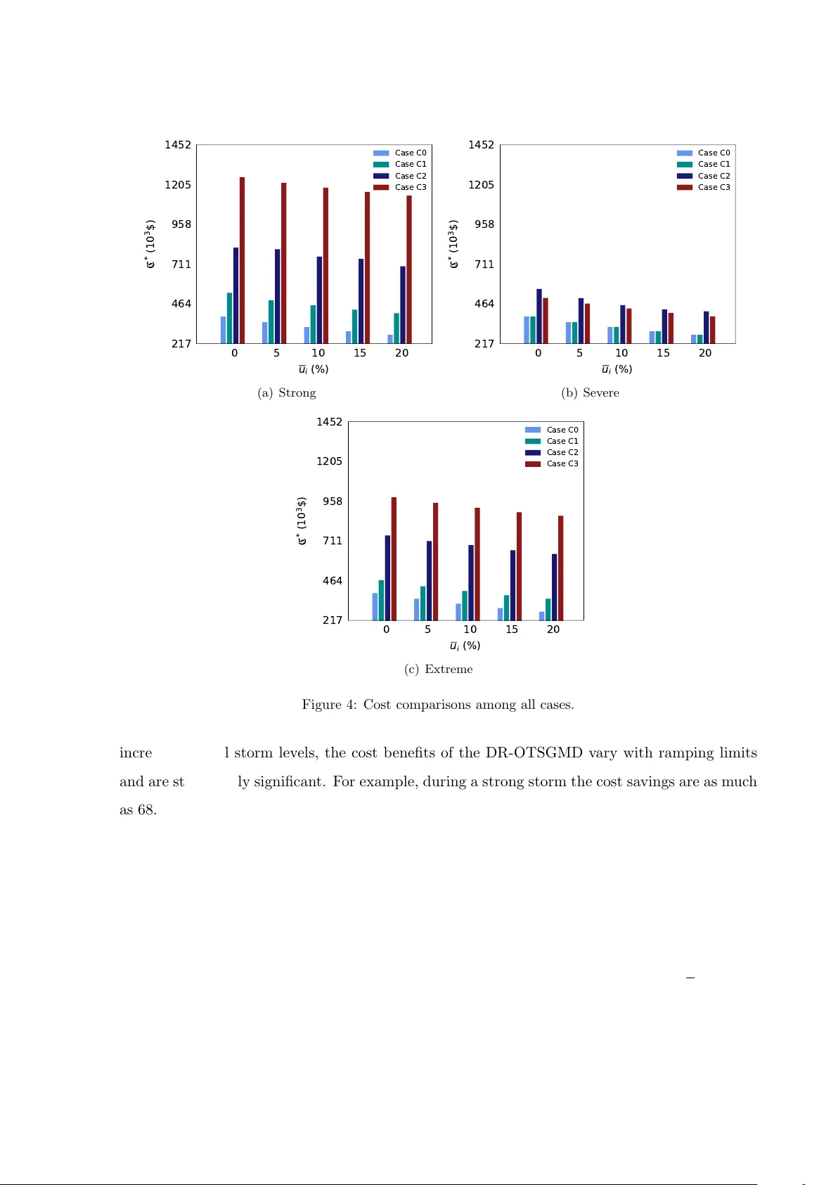
Distributionally Robust Optimization for a Resilien t T ransmission Grid During Geomagnetic Disturbances Mo wen Lu : , Sandra D. Eksioglu : , Scott J. Mason : , Russell Ben t ; , Harsha Nagara jan ; : Departmen t of Industrial Engineering, Clemson Univ ersit y , SC, United States. ; Applied Mathematics and Plasma Ph ysics Group (T-5), Los Alamos National Lab oratory , NM, United States. Abstract In recent years, there ha ve been increasing concerns about the impacts of geomagnetic disturbances (GMDs) on electrical p o wer systems. Geomagnetically-induced curren ts (GICs) can saturate transformers, induce hot-sp ot heating and increase reactiv e p o wer losses. Un- predictable GMDs caused by solar storms can signiﬁcantly increase the risk of transformer failure. In this pap er, we dev elop a tw o-stage, distributionally robust (DR) optimization form ulation that mo dels uncertain GMDs and mitigates the eﬀects of GICs on p ow er sys- tems through existing system con trols (e.g., line switching, generator re-dispatc h, and load shedding). This mo del assumes an ambiguit y set of probability distributions for induced geo-electric ﬁelds which capture uncertain magnitudes and orien tations of a GMD even t. W e emplo y state-of-the-art linear relaxation metho ds and reform ulate the problem as a tw o-stage DR mo del. W e use this formulation to develop a decomp osition framework for solving the problem. W e demonstrate the approach on the mo diﬁed Epri21 system and show that the DR optimization method eﬀectively handles prediction errors of GMD even ts. Key wor ds: distributionally robust optimization, uncertain GMDs, transmission line switc hing, linearizations, A C Po w er Flo w 1 In tro duction Solar ﬂares and coronal mass ejections form solar storms where charged particles escape from the sun, arriv e at Earth, and cause geomagnetic disturbances (GMDs). GMDs lead to c hanges in the Earth’s magnetic ﬁeld, which then create geo-electric ﬁelds. These low-fr equency , 1 geo-electric ﬁelds induce quasi-DC curren ts, also known as Geomagnetically-Induced Currents (GICs), in grounded sections of electric p o w er systems [1 – 3]. GICs are sup erimp osed on the existing alternating curren ts (AC) and bias the A C in transformers. This bias leads to half-cycle saturation and magnetic ﬂux loss in regions outside of the transformer core. The energy stored in the stra y ﬂux increases the reactive p ow er consumption of transformers, whic h can lead to load shedding since, in general, generators are not designed to handle suc h unexp ected losses. In addition, the stray ﬂux also driv es eddy currents that can cause excessive transformer heating. Excess heating leads to reduced transformer life and, p otentially , immediate damage [4]. As a result, when GMD ev ents o ccur on large-scale electric p ow er systems, the resulting p o wer outages can b e catastrophic. F or example, the GMD ev ent in Queb ec in 1989 led to the sh utdown of the Hydro-Queb ec p ow er system. As a consequence, six million p eople lost access to p ow er for nine hours. By some estimates the net cost of this ev ent was $ 13.2 million, with damaged equipment accoun ting for $ 6.5 million of the cost [5]. The potential GMD impacts to transformers in the bulk electric pow er system hav e mo- tiv ated the United States go vernmen t to sp onsor researc h to impro v e understanding of GMD ev ents and iden tify strategies for mitigating the impacts of GMDs on p ow er systems [6, 7]. T o mo del the p oten tial risks in tro duced b y GICs, research institutes and electric p ow er industries ha ve actively impro ved GIC modeling and GIC monitoring [8 – 12]. F or example, the North American Electric Reliability Corp oration (NERC) dev elop ed a pro cedure to quan tify GICs in a system based on the exp osure to geo-electric ﬁeld [13]. These mo dels are used to conduct risk analyses whic h estimate the sensitivit y of reactiv e p ow er losses from GICs. These studies indicate that risk mitigation warran ts further study . The recent literature mainly fo cuses on mitigating t wo risks introduced by GICs. The ﬁrst is voltage sag caused b y increased reactive p o wer consumption in transformers [4]. The second is transformer damage caused by excessive hot-sp ot thermal heating [14]. One mitigation is DC-curren t blo c king devices that preven t the GIC from accessing transformer neutrals [15]. Unfortunately , these devices are exp ensiv e; a single unit can cost $ 500K [16 – 18]. The high cost is a barrier to wide-scale adoption of this tec hnology . T o address this issue, Lu et al. [19] dev elop ed a GIC-aw are optimal AC p o wer ﬂow (A COPF) mo del that uses existing top ology con trol (line switching) and generator dispatch to mitigate the risks of GIC. This work show ed that top ology reconﬁguration can eﬀectively protect pow er systems from GIC impacts, whic h w as also later observed in [20]. Ho wev er, these pap ers assumed a deterministic GMD ev ent (i.e., the induced geo-electric ﬁeld is known). In reality , solar storms, such as solar ﬂares and coronal 2 mass ejections (CMEs), are diﬃcult to predict. Although ground- and space-based sensors and imaging systems hav e b een utilized by the National Aeronautics and Space Administration (NASA) to observe these activities at v arious depths in the solar atmosphere, the intensit y of a storm cannot b e measured until the released particles reac h Earth and interact with its geomagnetic ﬁeld [21]. As a result, there is often uncertaint y in predictions of solar storms and the induced geo-electric ﬁeld, whic h in tro duce op erational c hallenges for mitigating the potential risks b y GIC to p ow er systems. This pap er extends the study of GIC mitigation of [19] in tw o w ays. The mo del (1) uses line switching and generator ramping to mitigate GIC impacts and (2) assumes uncertain mag- nitude and orien tation of a GMD. W e form ulate this problem as a tw o-stage distributionally robust (DR) optimization model that we refer to as DR-OTSGMD. The ﬁrst-stage problem selects a set of transmission lines and generators to serve pow er in a p ow er system ahead of an imminen t GMD even t. The second-stage problem ev aluates the p erformance of the netw ork giv en the status of transmission lines, the reserv ed electricity for daily p ow er service, and a realized GMD. In this mo del, the uncertain magnitude and direction of a GMD are mo deled with an am biguit y set of probabilit y distributions of the induced geo-electric ﬁeld. The ob jectiv e is to minimize the exp ected total cost of the w orst-case distribution deﬁned in the ambiguit y set. Instead of assuming a sp eciﬁc candidate distribution, the ambiguit y set is describ ed b y statistical prop erties of uncertain ty , such as the supp ort and moment information. As a result, the DR optimization approac h yields less conserv ativ e solutions than prev alent robust optimiza- tion approaches [22, 23]. In comparison to stochastic programming, the DR metho d does not require complete information of the exact probability distribution, i.e., the decisions do not rely on assumptions ab out unkno wn distributions [24]. Additionally , the reliability of the solutions found w ith DR metho ds does not require a large n umber of random samples, whic h can lead to computational tractabilit y and scalabilit y issues for large-scale problems [25]. In the litera- ture, DR optimization approac hes hav e been used to mo del a v ariety of problems [26 – 31], such as con tingency-constrained unit commitment [22, 32, 33], optimal p o wer ﬂow with uncertain re- new able energy generation [25, 34 – 36], planning and sc heduling of pow er systems [37, 38], and energy managemen t [39, 40]. These observ ations and the lac k of studies ab out probabilit y dis- tributions for GMD ev ents mak es a DR mo del an attractiv e choice for mo deling uncertaint y in this problem. Given the computational complexit y (nonlinear ph ysics and trilev el mo deling) of this problem, we fo cus on dev eloping metho ds for computing DR op erating points based on lo wer b ounding techniques. T ec hniques for computing upp er b ound solutions and the globally 3 optimal solution are left for future w ork. The main con tributions of this pap er include: • A t w o-stage DR-OTSGMD mo del that captures the uncertaint y of the GMD-induced geo- electric ﬁeld. This formulation considers the AC ph ysics of p o wer ﬂo w and reactiv e p ow er consumption at transformers due to uncertain GICs. • A relaxation and reformulation of the tw o-stage DR-OTSGMD problem whic h facilitates the problem decomp osition and application of eﬃcient decomp osition algorithms. W e show that solutions of the resulting problem are a v alid lo wer b ound to the original problem. • Extensiv e numerical analysis using the Epri21 test system to v alidate the mo del and demon- strates its eﬀectiveness in generating robust solutions. The remainder of this pap er is organized as follo ws. In section 2.2.2, w e discuss the t w o-stage DR-OTSGMD form ulation and the ambiguit y set of probability distributions for the induced geo-electric ﬁeld. W e describe linear relaxations of nonlinear and non-con vex functions in the problem, then deriv e a decomp osition framework for solving the relaxation. In Section 3, we presen t a column-and-constraint generation algorithm and demonstrate the eﬀectiveness of the approac h using the Epri21 test system in Section 4. Finally , we conclude and provide directions for future research in Section 5. 2 Problem F orm ulation Here, we describe the DR-OTSGMD. W e ﬁrst introduce the AC pow er ﬂow model. W e then introduce the mo deling of the GIC. W e note that the A C and GIC ﬂows exist on the same ph ysical pow er system, how ever, they require diﬀerent representations of that system. The t wo representations are tied through deﬁned interactions of the A C and GIC currents. Third, we discuss the coupling b etw een the AC pow er ﬂow model and the GIC. Next, w e discuss the uncertain ty mo del. W e then discuss our conv ex (linear) relaxation of the problem and reform ulate this relaxation as a distributionally robust optimization problem. 2.1 Electric P o w er Mo del–AC The ob jective function for operating the A C electric pow er systems minimizes total gen- eration dispatc h cost as form ulated b y a quadratic function (1a). In this cost function, f p i denotes the real p o wer generation from generator i . The ﬁxed generation cost is incurred when 4 a generator is switched on (i.e., z g i “ 1). min ÿ i P G z g i c 0 i ` c 1 i f p i ` c 2 i p f p i q 2 (1a) The AC physics of electric p ow er systems are go v erned b y Kirc hoﬀ ’s and Ohm’s laws. Here, Kirchoﬀ ’s law is mo deled as constraints (2a)-(2b) and Ohms law is mo deled as constraints (2c)-(2f). ÿ e ij P E i p ij “ ÿ k P G i f p k ´ d p i ´ v 2 i g i @ i P N a (2a) ÿ e ij P E i q ij “ ÿ k P G i f q k ´ d q i ` v 2 i b i @ i P N a (2b) p ij “ 1 α 2 ij g e v 2 i ´ 1 α ij v i v j ` g e cos p θ i ´ θ j q ` b e sin p θ i ´ θ j q ˘ @ e ij P E a (2c) q ij “ ´ 1 α 2 ij p b e ` b c e 2 q v 2 i ` 1 α ij v i v j ` b e cos p θ i ´ θ j q ´ g e sin p θ i ´ θ j q ˘ @ e ij P E a (2d) p j i “ g e v 2 j ´ 1 α ij v i v j ` g e cos p θ j ´ θ i q ` b e sin p θ j ´ θ i q ˘ @ e ij P E a (2e) q j i “ ´p b e ` b c e 2 q v 2 j ` 1 α ij v i v j ` b e cos p θ j ´ θ i q ´ g e sin p θ j ´ θ i q ˘ @ e ij P E a (2f ) Here, p ij and q ij are the real and reactive ﬂo w b et ween buses i and j , as measured at no de i , resp ectiv ely . Similarly , f p j and f q j are the real and reactive generation at generator j and d p i and d q i are the real and reactiv e load at i . Finally , v i and θ i are the v oltage magnitude and phase angle at bus i , resp ectively . The ﬂow on lines is restricted by the ph ysical limits of the grid and are modeled with constrain ts (3a)-(3c). Constraints (3a) limit the v oltage magnitude at buses, while constrain ts (3b) apply b ounds on the phase angle diﬀerence b etw een tw o buses. Constraints (3c) model op erational thermal limits of lines at b oth sides. v i ď v i ď v i @ i P N a (3a) | θ i ´ θ j | ď θ @ e ij P E a (3b) p 2 ij ` q 2 ij ď s 2 e , p 2 j i ` q 2 j i ď s 2 e @ e ij P E a (3c) Generator outputs are limited b y the commitment of that generator and capacity upper and lo wer b ounds which are mo deled as constraints (4a)-(4c). Discrete v ariables z g i indicate the 5 generator’s on-oﬀ status and are incorp orated in to generator p o wer limits. z g i g p i ď f p i ď z g i g p i @ i P G (4a) z g i g q i ď f q i ď z g i g q i @ i P G (4b) z g i P t 0 , 1 u @ i P G (4c) F or mitigating GIC eﬀects, transmission lines are allow ed to b e switched on or oﬀ. W e mo del switc hing by mo difying constrain ts (2e)-(2f) and (3b)-(3c) with: p ij “ z a e ´ 1 α 2 ij g e v 2 i ´ 1 α ij v i v j ` g e cos p θ i ´ θ j q ` b e sin p θ i ´ θ j q ˘ ¯ @ e ij P E a (5a) q ij “ z a e ´ ´ 1 α 2 ij p b e ` b c e 2 q v 2 i ` 1 α ij v i v j ` b e cos p θ i ´ θ j q ´ g e sin p θ i ´ θ j q ˘ ¯ @ e ij P E a (5b) p j i “ z a e ´ g e v 2 j ´ 1 α ij v i v j ` g e cos p θ j ´ θ i q ` b e sin p θ j ´ θ i q ˘ ¯ @ e ij P E a (5c) q j i “ z a e ´ ´ p b e ` b c e 2 q v 2 j ` 1 α ij v i v j ` b e cos p θ j ´ θ i q ´ g e sin p θ j ´ θ i q ˘ ¯ @ e ij P E a (5d) z a e | θ i ´ θ j | ď θ @ e ij P E a (5e) p 2 ij ` q 2 ij ď z a e s 2 e , p 2 j i ` q 2 j i ď z a e s 2 e @ e ij P E a (5f ) z a e P t 0 , 1 u @ e P E a (5g) where z a e denotes the on-oﬀ status of transmission line e in the AC model. Constraints (5a)-(5d) mo del A C pow er ﬂo w on eac h line when the line is closed and force the ﬂo w to zero when the line is op en. Similarly , constrain ts (5e) and (5f) place phase angle diﬀerence limits and thermal limits on active lines, resp ectively . Giv en that generators can respond in a limited w ay to GIC, we mo del this resp onse with ramping constraints (6a)-(6b). Here, ρ i is the setp oin t of generator i P G . Constraints (6b) limit the deviation of real p ow er generation from ρ i when generator i is online. z g i g p i ď ρ i ď z g i g p i i P G (6a) | f p i ´ ρ i | ď z g i u R i g p i @ i P G (6b) The ob jectiv e function is then reformulated with the generator set p oints, i.e., min ÿ i P G z g i c 0 i ` c 1 i ρ i ` c 2 i p ρ i q 2 (7) 6 In addition, to ensure feasibility at all times, we introduce slack v ariables for ov er (i.e., l p ` i , l q ` i ) and under (i.e., l p ´ i , l q ´ i ) load consumption. This changes equations (2a)-(2b) to (8a)-(8b). ÿ e ij P E i p ij “ ÿ k P G i f p k ´ d p i ` l p ` i ´ l p ´ i ´ v 2 i g i @ i P N a (8a) ÿ e ij P E i q ij “ ÿ k P G i f q k ´ d q i ` l q ` i ´ l q ´ i ` v 2 i b i @ i P N a (8b) Similarly , the ob jective function is also mo diﬁed to p enalize the slackness with high cost ( κ i ), i.e., ÿ i P G z g i c 0 i ` c 1 i ρ i ` c 2 i p ρ i q 2 ` ÿ i P N a κ i p l p ` i ` l q ` i ` l p ´ i ` l q ´ i q (9) The slac k is in terpreted as an indication for the need to shed loads or to o ver generate. 2.2 Electric P o w er Mo del–GIC 2.2.1 r ν d e calculation The GIC calculation depends on induced voltage sources p r ν d e q on eac h p ow er line, e P E d , in the netw ork whic h are determined b y the geo-electric ﬁeld in tegrated along the transmission line. This relationship is mo deled in Eq. (10) r ν d e “ ¿ ~ E e ¨ d ~ l e , (10) where ~ E e is the geo-electric ﬁeld in the area of transmission line e P E d , and d ~ l e is the incremen tal line segment length including direction [13]. In practice, the actual geo-electric ﬁeld v aries with geographical lo cations. In this paper, w e use a common assumption that the geo-electric ﬁeld in the geographical area of a transmission line is uniformly distributed [12, 13, 17], i.e., ~ E “ ~ E e for an y e P E d . Hence, only the co ordinates of the line end p oin ts are relev an t and ~ E is resolv ed in to its east ward (x axis) and north ward (y axis) comp onen ts [13]. Given ~ L e , the length of line e with direction, equation (10) is reform ulated as: r ν d e “ ~ E ¨ ~ L e “ r ν N L N e ` r ν E L E e , @ e P E d (11) where r ν N and r ν E represen t the geo-electric ﬁelds (V/km) in the north ward and east ward di- rections, resp ectively . L N e and L E e denote distances (km) along the north ward and eastw ard directions, respectively , whic h dep end on the geographical lo cation (i.e., latitude and longi- 7 tude) [13]. 2.2.2 T ransformer mo deling The t wo most common transformers in electrical transmission systems are generator step-up (GSU) transformers and net w ork transformers. GSUs connect the output terminals of generators to the transmission net w ork. In con trast, netw ork transformers are generally lo cated relatively far from generators and transform voltage betw een diﬀerent sections of the transmission system. In this section, w e discuss how to mo del these tw o classes of transformers in the DC circuit induced by a GMD. F or notation brevity , we use subscripts h and l to represents the high- v oltage (HV) and low-v oltage (L V) buses of all transformers. Additionally , we deﬁne N x and I d x as the num b er of turns and GICs in the transformer winding x , resp ectiv ely , and let Θ p¨q denote a linear function of I d x . In this paper, w e model tw o types of GSU transformers: (1) GWye-Delta and (2) Delta- GWy e. Consisten t with common engineering practice, we assume that eac h GSU is grounded on the HV side that connects the generator to the transmission netw ork. Figure 1(a) shows the DC represen tation of the GSU transformer. It sho ws that the eﬀectiv e GICs (denoted as r I d ) dep end on GICs in the HV primary winding, i.e., r I d “ ˇ ˇ ˇ Θ p I d h q ˇ ˇ ˇ “ ˇ ˇ ˇ I d h ˇ ˇ ˇ (12) F or net work transformers, w e model (1) t wo-winding transformers: GWye-GWy e An to- and Gwy e-Gwye transformers and (2) three-winding transformers including Delta-Delta, Delta-Wy e, Wy e-Delta, and Wy e-Wye conﬁgurations. The DC-equiv alent circuits of GWye-GWy e An to- and Gwye-Gwy e transformers are shown in Figures 1(b) and 1(c), resp ectiv ely , where subscripts s and c denote the series and common sides of the auto-transformer. F or an auto-transformer, as sho wn in Figure 1(b), the eﬀec tiv e GICs are determined b y GIC ﬂows in the series and common windings, i.e., r I d “ ˇ ˇ ˇ Θ p I d s q ` Θ p I d c q ˇ ˇ ˇ “ ˇ ˇ ˇ p α ´ 1 q I d s ` I d c α ˇ ˇ ˇ (13) where turns ratio α “ N s ` N c N c . Similarly , the eﬀectiv e GICs for a Gwye-Gwy e transformer (Figure 1(c)) models GICs on the HV and L V sides, i.e., r I d “ ˇ ˇ ˇ Θ p I d h q ` Θ p I d l q ˇ ˇ ˇ “ ˇ ˇ ˇ αI d h ` I d l α ˇ ˇ ˇ (14) 8 where transformer turns ratio α “ N h N l . F or all three-winding transformers we assume that their windings are ungrounded. Hence, their asso ciated eﬀective GICs are zero b ecause ungrounded transformers do not provide a path for GIC ﬂow [13]. v d h v d l v d n a hn a nl = 0 high-side winding lo w-side winding I d h h l n a m (a) GWye-Delta/Delta-GWy e GSUs v d h a s a c a m v d n v d l I d s I d c series winding common winding h l n (b) GWye-GWy e Auto v d h v d l v d n a hn a nl high-side winding lo w-side winding I d h I d l h n l a m (c) Gwye-Gwy e Figure 1: DC equiv alent circuits for diﬀeren t types of transformers. h , l , and n (blue fon t) represent high-side bus, low-side bus, and neutral bus, resp ectively . 2.2.3 GIC Modeling The GMD-induced equiv alent DC circuit is mo deled through constrain ts (15a)-(15b). These constrain ts calculate the GIC ﬂo w on each line in the DC represenation of the ph ysical system. Equations (15a) model Kirchoﬀ ’s la w and equations (15b) mo del Ohm la w, where r ν d e denotes the DC-v oltage source of line e induced b y the geo-electric ﬁeld (see Section 2.2.1). ÿ e P E m I d e “ a m v d m @ m P N d (15a) I d e “ a e p v d m ´ v d n ` r ν d e q @ e mn P E d (15b) Constrain ts (16a)-(16b) mo del the eﬀectiv e GIC v alue of eac h transformer, r I d e , whic h de- p ends on the t yp e of transformer e P E τ . Instead of in tro ducing additional discrete v ariables, constrain ts (16a) mo del and relax the absolute value of ÿ p e ij P E w e Θ p I d p e q deﬁned in (12)–(14). This relaxation is often tight as larger DC current typically causes problems and drives the ob jective v alue up. Constrain t set (16b) denotes the maximum allow ed v alue of GIC ﬂowing through 9 transformers. W e assume this limit is twice the upp er b ound of the AC in the net work. r I d e ě ÿ p e ij P E w e Θ p I d p e q , r I d e ě ´ ÿ p e ij P E w e Θ p I d p e q @ e P E τ (16a) 0 ď r I d e ď max @ p e P E a 2 I a ˆ e @ e P E τ (16b) Constrain t set (17a) computes the reactiv e p ow er load due to transformer saturation [1, 11, 17, 41] by using the eﬀectiv e GICs for each transformer type. Here, d q loss i denotes the total reactiv e p ow er loads at bus i whic h is the high-voltage side of transformer e P E τ i . d q loss i “ ÿ e P E τ i k e v i r I d e @ i P N a (17a) Similar to the AC mo del, lines are switc hed on and oﬀ by mo difying constraints (15b) with on-oﬀ v ariables z d e as follo ws. I d e “ z d e a e p v d m ´ v d n ` r ν d e q @ e mn P E d (18a) z d e P t 0 , 1 u @ e P E d (18b) 2.3 Electric P o w er Mo del–Coupled GIC and A C The GIC and A C are tied in t wo w a ys. First, switching lines on and oﬀ impact b oth the A C and GIC formulation. W e use the AC switching v ariables (i.e., z a e and z g i ) and tie these v ariables to GIC switc hing by linking an edge e P N d in the DC circuit to an edge in the AC circuit and dropping the z d e v ariables. Sp eciﬁcally , for e P E d , we use Ý Ñ e to denote the asso ciated A C line of e . This is a one-to-one mapping for transmission lines and a man y-to-one mapping for transformers [19]. This is a one-to-one mapping for transmission lines and a man y-to-one mapping for transformers (i.e., both high and low-side windings of a transformer are linked to one and only one line in the AC circuit). Using this notation, constraints (18a) are mo diﬁed to constrain ts (19). I d e “ z a Ý Ñ e a e p v d m ´ v d n ` r ν d e q @ e mn P E d (19) Second, the reactive losses induced b y the GIC are added to the AC Kirchoﬀ equations b y 10 mo difying constrain ts (8b) to (20). ÿ e ij P E i q ij “ ÿ k P G i f q k ´ d q i ´ d q loss i ` l q ` i ´ l q ´ i ´ v 2 i b i @ i P N a (20) 2.4 A Tw o-stage OTSGMD Model Assuming that the induced geo-electric ﬁeld is constan t (i.e., r ν d e are kno wn parameters), the OTSGMD problem is deterministic and it is natural to formulate the problem with tw o stages. In the ﬁrst stage, generator setp oin ts and the on/oﬀ status of generators and edges are determined prior to an imminent GMD even t. The second stage determines op erational decisions of the p ow er system in resp onse to the giv en ev ent. The formulation of this t wo-stage OTSGMD model is presented with: min ÿ i P N g z g i c 0 i ` c 1 i ρ i ` c 2 i p ρ i q 2 ` H p z a , z g , ρ , r ν d q (21a) s.t. (4c) , (5g) , (6a) (21b) Where H p z a , z g , ρ , r ν d q “ min ÿ i P N g c R 2 i p ∆ p i q 2 ` c R 1 i ∆ p i ` ÿ i P N a κ i p l p ` i ` l q ` i ` l p ´ i ` l q ´ i q (22a) s.t. ∆ p i ě 0 , ∆ p i ě f p i ´ ρ i @ i P G (22b) (3a) , (4a) ´ (4b) , (5a) ´ (5f) , (6b) , (8a) , (11) , (15a) , (16a) ´ (17a) , (19) ´ (20) (22c) The ﬁrst-stage problem (21) speciﬁes a system top ology and real-p ow er generation set p oin ts for daily electricit y consumption. The ob jective function (21a) minimizes the total cost including the ﬁxed cost for keeping generators on, the fuel cost for the settled generator outputs, and the op erating cost H p z a , z g , ρ , r ν d q of the second stage. The second-stage problem is formulated as (22) which minimizes H p z a , z g , ρ , r ν d q as function of the fuel cost for the ramp-up generation and a p enalt y for o v er and under load. Constrain ts (22b) mo del the ramp-up generation (i.e., p ositiv e deviation) of real p o wer at each generator. If generator i P G ramps up, the minim um ∆ p i is equal to f p i ´ ρ i ; 0 otherwise. Note that the cost function (22a) tak es in to account only the ramp-up p ow er generation, th us there is no cost if generator i P G ramps do wn. 11 2.5 A Tw o-stage DR-OTSGMD Model with Uncertain t y In practice, solar storms are unpredictable, whic h in turn leads to uncertain geo-electric ﬁelds ~ E . Speciﬁcally , the north ward and eastw ard geo-electric ﬁelds (V/km), r ν N and r ν E , are random v ariables and aﬀect the induced voltage sources on transmission lines ν d e as equation (11). Hence, w e replace the ob jective function (21a) with its exp ectation equiv alen t as follo ws: Q o : “ min ÿ i P N g z g i c 0 i ` c 1 i ρ i ` c 2 i p ρ i q 2 ` sup P P Q E P r H p z a , z g , ρ , r ν d qs (23) Where sup P P Q E P r H p z a , z g , ρ , r ν d qs is the worst-case exp ected op erating cost incurred in the second stage ov er an ambiguit y set Q of an unknown probabilit y measure P of random v ariables r ν N and r ν E , whic h w e discuss in detail in Section 2.7. 2.6 Con v ex Relaxations The tw o-stage DR-OTSGMD mo del is a v ery hard mixed-integer non-con vex problem be- cause of constrain ts (5a)-(5d), (8a), (8b), (17a), and (19)-(20). One of the fo cuses of this pap er is the deriv ation of lo wer b ounds to DR-OTSGMD, so we relax each of these constraints. F or notation brevity , in the follo wing sections, L x denotes a set of uniformly located p oin ts within the bounds of the v ariable x . Quadratic F uel Cost F unction. In this paper, the fuel cost is form ulated as a quadratic function of the real p o wer generation from generator i P G (i.e., c 1 i ρ i ` c 2 i p ρ i q 2 ). By applying the p ersp ective reform ulation describ ed in [42 – 44], the quadratic term c 2 i p ρ i q 2 is reform ulated as: z g i q ρ i ě ρ 2 i @ i P G (24) Constrain ts (24) guaran tees that the minim um (optimal) v alue of q ρ i is zero if generator i is switc hed oﬀ (i.e., z g i “ 0). Otherwise q ρ i is equal to ρ 2 i when z g i “ 1 because this is a minimization problem. Next, we replace constrain ts (24) with a set of piecewise linear constraints whic h outer appro ximate (relax) q ρ i as follo ws: q ρ i ě 2 ρ i ` ´ z g i p ` q 2 @ i P N g , ` P L ρ i (25) Constrain ts (25) describ e a set of linear inequalities that are tangent to the quadratic curve ρ 2 i 12 at points l P L ρ i . As a result, the ob jectiv e function is mo diﬁed as follows. min ÿ i P N g z g i c 0 i ` c 1 i ρ i ` c 2 i q ρ i ` sup P P Q E P r H p z a , z g , ρ , r ν d qs (26) Similarly , we use the same metho d to relax the quadratic term ∆ 2 i and replace equations (22) with equations (27). H p z a , z g , ρ , r ν d q “ min ÿ i P G c R 2 i q ∆ i ` c R 1 i ∆ i ` ÿ i P N a κ i p l p ` i ` l q ` i ` l p ´ i ` l q ´ i q (27a) q ∆ i ě 2 ` p ∆ i q ´ z g i p ` q 2 @ i P N g , ` P L ∆ i (27b) A C P ow er Flow Ph ysics. In constrain ts (5a)-(5d), (8a) and (20), the nonlinearities are expressed with the following terms [45]: p 1 q w i : “ v 2 i , p 2 q w z ie : “ z e v 2 i p w z j e : “ z e v 2 j q , p 3 q w c e : “ z e v i v j cos p θ i ´ θ j q , p 4 q w s e : “ z e v i v j sin p θ i ´ θ j q The auxiliary v ariables w i , w z ie , w z j e , w c e and w s e are introduced to relax each of these quantities. First, the quadratic term w i : “ v 2 i , is con v exiﬁed b y applying the second-order conic (SOC) relaxation deﬁned in equation (29). w i ě v 2 i @ i P N a (29a) w i ď p v i ` v i q v i ´ v i v i @ i P N a (29b) F urther, we outer appro ximate (relax) the conv ex env elope of v 2 i using a set of piecewise linear constrain ts which replace constrain ts (29a) with constrain ts (30): w i ě 2 `v i ´ p ` q 2 @ i P N a , ` P L v i (30) Next, to relax non-conv ex constraints w z ie : “ z e v 2 i and w z j e : “ z e v 2 j , w e introduce the follow- ing notation: Giv en any tw o v ariables x i , x j P R , the McCormick (MC) relaxation [46] is used to relax a bilinear product x i ¨ x j b y in tro ducing an auxiliary v ariable x ij P x x i , x j y M C . The feasible region of x ij is giv en b y: x ij ě x i x j ` x j x i ´ x i x j (31a) x ij ě x i x j ` x j x i ´ x i x j (31b) x ij ď x i x j ` x j x i ´ x i x j (31c) 13 x ij ď x i x j ` x j x i ´ x i x j (31d) x i ď x i ď x i , x j ď x j ď x j (31e) Applying the relaxations in (29) to v 2 i and v 2 j , results in auxiliary v ariables, w i and w j , resp ec- tiv ely . Thus, the constrain ts w z ie : “ z e v 2 i and w z j e : “ z e v 2 j can b e expressed as w z ie : “ x z e , w i y M C and w z j e : “ x z e , w j y M C , resp ectiv ely . It is also imp ortant to notice that the MC relaxation is exact when one v ariable in the pro duct is binary [47]. Finally , to deal with nonlinear terms w c e : “ z e v i v j cos p θ i ´ θ j q and w s e : “ z e v i v j sin p θ i ´ θ j q , though there are numerous tight con v ex relaxations in the literature [48 – 52], we apply state- of-the-art SOC relaxations of [53] considering it’s computational eﬀectiv eness, as formulated in constrain ts (32). z e w c e ď w c e ď z e w c e , z e w s e ď w s e ď z e w s e @ e ij P E a (32a) tan p θ q w c e ď w s e ď tan p θ q w c e @ e ij P E a (32b) p w c e q 2 ` p w s e q 2 ď w z ie w z j e @ e ij P E a (32c) Note that constrain t set (32b) is equiv alent to the phase angle limit constrain ts (3b). Constraint set (32c) is the SOC relaxations of equation z a e ` p w c e q 2 ` p w s e q 2 ´ w i w j ˘ “ 0 whic h is obtained b y linking w c e and w s e through the trigonometric iden tit y cos 2 p θ i ´ θ j q ` sin 2 p θ i ´ θ j q “ 1. F urther, we use a set of piecewise linear constrain ts to outer appro ximate (relax) the rotated SOC constrain ts (32c) suc h that: 2 ´ w c e ` c ` w s e ` s ¯ ´ w z ie ` t ´ w z j e ` f ď z e ` p ` c q 2 ` p ` s q 2 ´ ` f ` t ˘ @ e ij P E a ` c P L w c e , ` s P L w s e , ` f P L w i , ` t P L w j (33) Based on these relaxations, w e replace the non-con vex constraints in (5a)-(5d), (8a) and (20) with constrain ts (34). Constrain ts (34c)–(34f) force line ﬂo ws to b e zero when the line is switc hed-oﬀ and tak e the asso ciated v alues otherwise. ÿ e ij P E ` i p ij ` ÿ e j i P E ´ i p ij “ ÿ k P G i f p k ` l p ` i ´ l p ´ i ´ d p i ´ w i g i @ i P N a (34a) ÿ e ij P E ` i q ij ` ÿ e j i P E ´ i q ij “ ÿ k P G i f q k ` l q ` i ´ l q ´ i ´ d q i ´ d q loss i ` w i b i @ i P N a (34b) 14 p ij “ g e w z ie ´ g e w c e ´ b e w s e @ e ij P E a (34c) q ij “ ´p b e ` b c e 2 q w z ie ` b e w c e ´ g e w s e @ e ij P E a (34d) p j i “ g e w z j e ´ g e w c e ` b e w s e @ e ij P E a (34e) q j i “ ´p b e ` b c e 2 q w z j e ` b e w c e ` g e w s e @ e ij P E a (34f ) w z ie : “ x z e , w i y M C , w z j e : “ x z e , w j y M C @ e ij P E a (34g) (29b) , (30) , (32a) ´ (32b) , (33) (34h) Line Thermal Limits. Similar to constraints (30), w e replace constrain ts (5f) with (35) which outer appro ximate (relax) quadratic terms p 2 ij ` q 2 ij and p 2 j i ` q 2 j i . 2 p ij ` p ` 2 q ij ` q ď z a e ` s 2 e ` p ` p q 2 ` p ` q q 2 ˘ @ e ij P E a , ` p P L p e , ` q P L q e (35a) 2 p j i ` p ` 2 q j i ` q ď z a e ` s 2 e ` p ` p q 2 ` p ` q q 2 ˘ @ e ij P E a , ` p P L p e , ` q P L q e (35b) GIC-Asso ciated Eﬀects. In the second stage, given geo-electric ﬁelds induced by a realized GMD, all nonlinearities and non-conv exities are in the bilinear form as: (1) z a Ý Ñ e p v d m ´ v d n q , and (2) v i I d e . Using MC relaxations as describ ed in (31), w e replace constrain ts (17a) with (36a)-(36b) and replace constraints (19) with (36c)-(36d). d q loss i “ ÿ e P E τ i k e u d ie @ i P N a (36a) u d ie P x v i , p I d e y M C @ i P N a , e P E τ i (36b) I d e “ a e v z d mn ` z a Ý Ñ e a e r ν d e @ e mn P E d (36c) v z d mn P x z g Ý Ñ i , v d m ´ v d n y M C @ e mn P E d (36d) where v z d mn and u d ie are in tro duced as v z d mn : “ z a Ý Ñ e p v d m ´ v d n q and u d ie : “ v i I d e . 2.7 Mo del of Uncertain t y This section fo cuses on constructing an ambiguit y set (denoted by Q ) of probabilit y distri- butions for the random geo-electric ﬁeld induced by a GMD ev en t. The notation r ω is used to denote the v ector of all random v ariables (i.e., r ω “ r r ν E , r ν N s T ) and the notation µ “ r µ E , µ N s T is used to denote the mean v ector of the east w ard and north w ard geo-electric ﬁelds. The am biguit y set Q is then formulated with: 15 Q “ $ ’ ’ ’ ’ ’ & ’ ’ ’ ’ ’ % r ω P R 2 P P P 0 p R q : E P p r ω q “ µ P ´ r ω P Ω ¯ “ 1 (37) where P 0 p R q denotes the set of all probability distributions on R and P denotes a probabilit y measure in P 0 . It is important to note that random v ariables r ω are not asso ciated with an y sp eciﬁc probability distribution. The second line of equation (37) forces the expectation of r ω to be µ . The third line deﬁnes the support of the random v ariables, Ω, and contains all the p ossible outcomes of r ω . W e form ulate this supp ort set based on v alid bounds of geo-electric ﬁelds in eastw ard and northw ard directions, suc h that: Ω : “ ! p r ν N , r ν E q P R : 0 ď r ν N ď ν M , ´ ν M ď r ν E ď ν M , p r ν N q 2 ` p r ν E q 2 ď p ν M q 2 ) (38) As introduced in Section 2.2.1, the geo-electric ﬁeld Ý Ñ E is form ulated as a vector and represen ted b y its t w o components r ν E and r ν N . Here, w e assume the direction of Ý Ñ E is orientated from 0 ° to 180 ° . The ﬁrst tw o constrain ts in Ω deﬁne individual b ounds of r ν N and r ν E , resp ectively . Giv en a presp eciﬁed upp er b ound on the geo-electric ﬁeld amplitude (denoted by ν M ), the third inequalit y further limits the feasible v alues of r ν N and r ν E whic h is form ulated as a quadratic constrain t and inferred by the geometric representation of Ý Ñ E . T o b etter demonstrate set Ω, ﬁgure 2 giv es tw o examples that illustrate feasible domains of r ν E and r ν N , where v ector ~ E represen ts the geo-electric ﬁeld in the area of a transmission system. In the ﬁgure, the half circle represen ts the quadratic b oundary of ~ E (i.e., p r ν E q 2 ` p r ν N q 2 ď p ν M q 2 ) E W e ν N ~ E e ν E N (a) r ν E ă 0, | ~ E | “ ν M E N W e ν N e ν E ~ E (b) r ν E ą 0, | ~ E | ă ν M Figure 2: Examples of feasible regions of r ν E and r ν N . The geo-electric ﬁeld ~ E is formed by r ν E and r ν N . In Fig. 2(a), the magnitude of ~ E equals ν M and angle relative to east is larger than π 2 . In Fig. 2(b), the magnitude of ~ E is less than ν M and the angle is smaller than π 2 . 16 2.8 Reform ulation of the Tw o-Stage DR-OTSGMD Using the relaxation methods describ ed in Section 2.6, the subproblem is linear and is a lower b ound of the original ob jectiv e. Adopting the notation of [32], we present the linearized program in a succinct form as follo ws: min y a T y ` sup P P Q E P r H p y , r ω qs (39a) Ay ě b (39b) where H p y , r ω q “ min x c T x (39c) s.t. Gy ` E x ě h (39d) T p r ω q y “ W x (39e) where y denotes the ﬁrst-stage v ariables and x denotes the second-stage recourse v ariables that dep end on random v ariables r ω “ r r ν E , r ν N s T . Constrain t set (39b) represen ts constrain ts (6a) and (25) in standard form. Constraint set (39d) represents constrain ts (3a), (4a)-(4b), (6b), (15a), (16), (22b), (34)-(36). Constraint set (39e) represents constraints (11) and (36c) that are the equations that include random v ariables in the problem. Here, T p r ω q is an aﬃne function of r ω such that T p r ω q “ ř | r ω | i “ 1 T i r ω i . In the rest of this section, w e deriv e a reform ulation of the t wo-stage DR-OTSGMD problem which can b e solved by applying a decomp osition framework. 2.8.1 Handling the w orst-case exp ected cost According to Zhao and Jiang [32], an equiv alen t problem to (39) rewrites the w orst-case exp ected cost sup P P Q E P r H p y , r ω qs in the ob jectiv e function (39a) as problem (40). sup P P Q E P r H p y , r ω qs “ max P ż Ω H p y , r ω q P p d r ω q (40a) s.t. ż Ω r ω P p d r ω q “ µ (40b) ż Ω P p d r ω q “ 1 (40c) Here, constrain ts (40b)–(40c) precisely describ e the am biguit y set deﬁned in (37). Constraint (40b) deﬁnes the mean v alue of random v ariables r ω . Equation (40c) form ulates the supp ort set Ω whic h con tains all the p ossible outcomes of r ω . Then, based on duality theory [54], the problem 17 is equiv alen tly reform ulated as (41) by incorp orating the dual problem of (40) in form ulation (39). Q d : “ min y , λ ,η a T y ` µ T λ ` η (41a) s.t. (39b) η ě H p y , r ω q ´ λ T r ω @ r ω P Ω (41b) where H p y , r ω q “ min x c T x : Gy ` E x ě h , T p r ω q y “ W x ( (41c) where λ and η are dual v ariables asso ciated with constraints (40 b ) and (40 c ), resp ectively . In addition, since constraints (41b) m ust b e satisﬁed for all realizations of r ω o v er support Ω, the equiv alent formulation of constraints (41b) is expressed as: η ě max @ r ω P Ω H p y , r ω q ´ λ T r ω ( (42) F urther, by applying standard duality theory , the right-hand side of constraint (42) is rewritten as the inner maximization problem: max @ r ω P Ω ! H p y , r ω q ´ λ T r ω ) “ max @p γ , π qP Γ , r ω P Ω ! p h ´ Gy q T γ ` y T ` | r ω | ÿ i “ 1 p T i q T π r ω i ˘ ´ λ T r ω ) (43a) Γ “ $ & % E T γ ` W T π ď c γ ě 0 (43b) where γ and π are dual v ariables asso ciated with constrain ts (39d) and (39e), resp ectively . Γ denotes the feasible domain of the dual v ariables. 2.8.2 Relaxing bilinear terms in the reformulation F or ﬁxed y and λ , the ob jectiv e function (43a) contains bilinear terms π r ω i . The liter- ature presen ts sev eral metho ds to solv e robust optimization (RO) mo dels with bilinear terms in the inner (sub-) problem, including heuristics [55] and mixed-integer programming (MIP) reform ulations [56 – 58]. The former ﬁnds lo cal optima for t w o-stage robust problems for which the uncertaint y set is a general p olyhedron (e.g., non-conv ex regular p olyhedra [59]). The latter ﬁnds exact solutions for R O problems by exploiting the sp ecial structure of the uncertaint y set. 18 A recen t w ork by Zhao and Zeng [23] dev elops an exact algorithm for tw o-stage R O problems for which the uncertain t y set is a general p olyhedron. The authors derive an equiv alen t MIP form ulation for the inner problem b y using strong Karush–Kuhn–T uck er (KKT) conditions. Ho wev er, this MIP formulation is c hallenging to solv e when binary v ariables are in tro duced to linearize complementary slackness constraints. Hence, it is diﬃcult to derive exact solutions for R O mo dels for whic h the uncertain ty set is a general polyhedron. Thus, w e lea ve the exploration of exact solution methods as future w ork. In this researc h, we focus on generating a lo wer b ound for the reformulation of Q d describ ed in (41). F rom formulation (43), we observe that r ω only app ears in the ob jective function (43a), th us diﬀerent realizations of r ω do not aﬀect the feasible region of the dual v ariables, Γ (43b). W e note that Γ is nonempty , since formulation (41c) is feasible for any given ﬁrst-stage solution due to load shedding and ov er-generation options. Let p p π , p γ q P Γ be an y feasible dual solution to form ulation (43). It follows that p y and p λ are solutions of ﬁrst-stage v ariables y and λ , resp ectiv ely . Giv en a solution p y , p λ , p π and p γ , the maximum v alue of (43a) is the optimal ob jectiv e v alue of (44) where r ω are the only decision v ariables: max @ r ω P Ω ! p h ´ G p y q T p γ ` p y T ` | r ω | ÿ i “ 1 p T i q T p π r ω i ˘ ´ p λ T r ω ) (44) Based on LP geometry [54, 60], if Ω is a b ounded and nonempty p olyhedron, then there exists an optimal (w orst-case) solution of r ω which is an extreme p oin t of Ω. Ho wev er, as describ ed in Eq. (38), Ω is conv ex set b ounded by a quadratic curve that has an inﬁnite num b er of extreme p oin ts. Thus, we discretize the curve and create a p olyhedral supp ort set Ω 1 that is b ounded by a piecewise linear relaxation of the curve. Hence, w e mo dify formulation (44) to b e (45). Under this form ulation there m ust b e a v ertex of Ω 1 whic h is an optimal r ω for (45). max @ r ω P Ω 1 ! p h ´ G p y q T p γ ` p y T ` | r ω | ÿ i “ 1 p T i q T p π r ω i ˘ ´ p λ T r ω ) (45) W e formalize the prop erties of Ω 1 with Lemma 2.1. Lemma 2.1. Given that Ω 1 is a line ar r elaxation of Ω and Ω 1 P Ω . Then, for any given ﬁrst- stage de cisions y and λ , ther e exists an extr eme p oint of Ω 1 which is an optimal (worst-c ase) solution of r ω P Ω 1 . Pr o of. Giv en that Ω is bounded and nonempt y as deﬁned in (38) and Ω is part of a max function 19 in a minimization problem, Ω 1 is a linear relaxation of Ω. As illustrated in Figure 3, Ω 1 is a nonempt y p olyhedron that is b ounded by linear cuts going through a series of p oints on the curv e (i.e., the b oundary of Ω). Then, for ﬁxed decisions p y and p λ , the problem (45) is a linear programming problem of ﬁnding the w orst-case p ω o ver a nonempt y and b ounded p olyhedron Ω 1 . Th us, based on LP geometry [54, 60], there exists an extreme p oint of Ω 1 whic h is optimal. . E N W ω ∗ 1 ω ∗ 2 ω ∗ 3 ω ∗ 4 ω ∗ 5 Figure 3: A linear relaxation of supp ort set Ω. The blue shadow represen ts Ω 1 and ω ˚ i for i P t 1 , 2 , .., 5 u denote the v ertices of Ω 1 . 2.8.3 A MIP reform ulation of the t w o-stage DR O-OTSGMD problem Based on prop osition 2.1, w e deriv e a MIP form ulation (denoted as Q v ) by introducing binary v ariables associated with eac h extreme p oint of Ω 1 . The formulation is describ ed as follo ws. Q v : “ min y , λ ,η a T y ` µ T λ ` η (46a) s.t. (39b) where η ě max γ , π , r ω p h ´ Gy q T γ ` y T ` | r ω | ÿ i “ 1 | K | ÿ j “ 1 p T i q T ζ j r ω ˚ ij ˘ ´ λ T r ω (46b) s.t. E T γ ` W T π ď c (46c) γ ě 0 (46d) ζ j l P x β j , π l y M C @ j P K , @ l P t 1 , ..., |p 39 e q|u (46e) r ω “ | K | ÿ j “ 1 β j r ω ˚ j (46f ) 20 | K | ÿ j “ 1 β j “ 1 (46g) β j P t 0 , 1 u , @ j P K (46h) where K is the set of v ertices (denoted as r ω ˚ ) of set Ω 1 β j are binary v ariables used to con trol the selection of an extreme p oin t r ω ˚ j . ζ j are contin uous v ariables introduced for linearizing bilinear pro ducts β j π via McCormic k Relaxations as described in (31). Note that this linearization is exact due to β j P t 0 , 1 u [61, 62]. The underlying idea of this MIP mo del is that we only consider the extreme p oints of Ω as candidate solutions for r ω . Hence, for any given ﬁrst-stage decision p y , λ q , the resulting w orst-case r ω is a vertex of Ω 1 . Since K collects the vertices of Ω 1 and K ‰ H , lemma 2.1 pro ves that there exists a vertex p ω ˚ j P K which is the w orst-case scenario of p ω P Ω 1 , suc h that: max @ r ω P K H p y , r ω q ´ λ T r ω ( “ max @ r ω P Ω 1 H p y , r ω q ´ λ T r ω ( (47) In other w ords, we reduce the feasible set of p ω to a series of extreme p oints in K and solve the reform ulation Q v in (46) to identify the minimum w orst-case expected total cost. Recall that form ulation (41) (denoted as Q d ) minimizes the w orst-case exp ected total cost ov er am biguity set Ω. Th us, the optimal solution of problem Q v (46) is less than the minim um cost obtained b y solving Q d , as Ω 1 is a subset of Ω. In addition, since the initial DR-OTSGMD mo del Q o is nonlinear and model Q d is a linear relaxation of Q o as describ ed in Section 2.6, the optimal solution of Q d is a lo wer bound of Q o . Ov erall, Q v returns a lo wer bound of Q d , while Q d generates a lo wer b ound of Q o . W e prov e this conclusion in prop osition 1 and 2 as follows. Prop osition 1. The worst-c ase exp e cte d total c ost obtaine d fr om formulation Q v is a lower b ound to the r eformulate d two-stage DR-OTSGMD pr oblem Q d . Pr o of. Let Q ˚ d and Q ˚ v b e the optimal ob jectiv e v alues to form ulations Q d and Q v , respectively . η ˚ d and η ˚ v represen t the optimal v alues of η to mo dels Q d and Q v , respectively . Since K represen ts the v ertexes of Ω 1 , then K Ď Ω 1 Ď Ω and the following holds: max @ r ω P Ω H p y , r ω q ´ λ T r ω ( ě max @ r ω P K H p y , r ω q ´ λ T r ω ( (48) As a result, for any given ﬁrst-stage decisions y and λ , the following is true: a T y ` µ T λ ` η ˚ d ě a T y ` µ T λ ` η ˚ v (see constrain ts (41b) and (46b)), i.e., Q ˚ v ď Q ˚ d . 21 Prop osition 2. Solving formulation Q v yields a lower b ound of the worst-c ase exp e cte d total c ost to the two-stage DR-OTSGMD pr oblem Q o . Pr o of. Let Q ˚ o , Q ˚ d , and Q ˚ v b e the optimal ob jectiv e function v alues of formulations Q o , Q d , and Q v , resp ectively . As described in Section 2.6, Q d is a linear relaxation of Q o . Hence, Q d yields a low er b ound for Q o , i.e., Q ˚ d ď Q ˚ o . F urther, Q ˚ v ď Q ˚ d based on prop osition 1. Th us, Q ˚ v ď Q ˚ d ď Q ˚ o . 3 Solution Metho dology: A column-and-constrain t generation algorithm T o solv e the t wo-stage DR-OTSGMD problem, we use the column-and-constraint generation (C&CG) algorithm describ ed in [57]. Similar to Benders’ decomp osition, the C&CG algorithm is a cutting plane metho d. It iterativ ely reﬁnes the feasible domain of a problem b y sequen tially generating a set of recourse v ariables and their asso ciated constraints. The algorithmic descrip- tion of the C&CG pro cedure is presen ted in Algorithm 1. In this algorithm, the notation O is used to denote a subset of K . LB and UB represen t incum b ent low er and an upp er b ounds of form ulation (46), resp ectively . Here,  is a suﬃciently small p ositiv e constant used to determine con vergence. Lines 3-10 are the main b o dy of the C&CG and they describ e a cutting plane pro cedure for the ﬁrst K iterations. In lines 4-5, the LB is ev aluated during iteration K using the incumbent solution p y K ` 1 , p λ K ` 1 and p η K ` 1 . Note that in the initial iteration ( K “ 0), set O is empty and master problem P p¨q lacks constraints (49a)-(49c). In lines 6-7, the subproblem Q p¨q is solved, the UB is estimated, and the w orst-case scenario p r ω K ` 1 is generated using the incum b ent decision ( p y K ` 1 , p λ K ` 1 ). Line 8 generates a new set of recourse v ariables x K ` 1 and asso ciated constrain ts (51) for P p¨q . Note that constrain t (51a) is v alid only if subproblem Q p¨q is b ounded (i.e., complete recourse). Line 9 expands set O and adds these newly-generated v ari- ables and constraints to the master problem P p¨q to tighten the feasible domain of the ﬁrst-stage v ariables (line 4). The pro cess is rep eated un til the ob jective v alues of the upp er and low er b ound con verge (line 3). Note that the optimal solution of the relaxed reform ulation (46) is obtained b y en umerating all the p ossible uncertain scenarios (v ertexes) in K . How ever, even though the n umber extreme p oin ts is linear in the problem size, full en umeration is computationally intractable when subset K is large. One adv antage of the C&CG is that the computational eﬀorts is often signiﬁcan tly 22 Algorithm 1 Column-and-Constraint Generation (CCG) 1: function CCG 2: Set K Ð 0, LB Ð ´8 , U B Ð `8 , O “ H 3: while | U B ´ LB | LB ď  do 4: Solv e the follo wing master problem P p p r ω P O q “ min y , λ ,η, x a T y ` µ T λ ` η s.t. p 39 b q η ě c T x l ´ λ T p r ω l @ l ď K (49a) Gy ` E x l ě h @ l ď K (49b) T p p r ω l q y “ W x l @ l ď K (49c) 5: Use the optimal solution p y K ` 1 , p λ K ` 1 and p η K ` 1 to calculate LB Ð P p p r ω P O q 6: Solv e Q p p y K ` 1 , p λ K ` 1 q “ max γ , π , r ω p h ´ G p y K ` 1 q T γ ` p p y K ` 1 q T ` | r ω | ÿ i “ 1 | K | ÿ j “ 1 p T i q T ζ j r ω ˚ ij ˘ ´ p p λ K ` 1 q T r ω (50a) s.t. p 46 c q ´ p 46 h q 7: Use the optimal solution p r ω K ` 1 to calculate U B Ð LB ´ p η K ` 1 ` Q p p y K ` 1 , p λ K ` 1 q 8: Generate a new set of recourse v ariables x K ` 1 and the following constraints for P p¨q η ě c T x K ` 1 ´ λ T p r ω K ` 1 (51a) Gy ` E x K ` 1 ě h (51b) T p p r ω K ` 1 q y “ W x K ` 1 (51c) 9: Up date O Ð O Ť p r ω K ` 1 and K Ð K ` 1 10: end while 11: return p y K ` 1 12: end function reduced by using a partial en umeration of non-trivial scenarios of the random v ariables r ω . Additionally , the C&CG algorithm is known to conv erge in a ﬁnite n umber of iterations since the n umber of extreme p oints in K is ﬁnite [23]. 4 Case Study This section analyzes the p erformance of our approac h on a p o wer system that is exposed to uncertain geo-electric ﬁelds induced b y GMDs. W e use a mo diﬁed v ersion of the Epri21 sys- tem [63]. The size of this net work is comparable to previous w ork [17] that considered minimiza- tion of quasi-static GICs and did not consider A COPF with top ology con trol. Computational exp erimen ts were p erformed using the HPC P almetto cluster at Clemson Univ ersit y with In tel 23 Xeon E5-2665, 24 cores and 120GB of memory . All algorithms and mo dels are implemented in Julia using using JuMP [64]. All problems are solved using CPLEX 12.7.0 (default options). 4.1 Data Collection and Analysis The main source of historical data for GMDs is recent w ork b y W o o droﬀe et al. [65]. The authors analyzed 100 y ears of data related to storms and their pap er indicates that the magnitude of the corresp onding induced geo-electric ﬁelds v aries with the magnetic latitudes. The authors also categorized geomagnetic storms in to three classes, strong, sev ere and extreme, according to the range of geo electromagnetic disturbances (Dst). T able 1 summarizes parameters used for describing the uncertain electric ﬁelds induced by GMDs. In this table, ν M denotes the maxim um amplitude of geo-electric ﬁelds induced b y GMDs (see Section 2.7). Its v alue is based on a 95% conﬁdence in terv al (CI) of 100-y ear p eak GMD magnitudes [65] (T able 1-3 in [65]). The v alues of µ N and µ E are estimated via extreme v alue analysis of electric ﬁelds from 15 geomagnetic storms using a Generalized Extreme V alue Distribution mo del for b oth north ward and east ward comp onen ts (i.e., r ν N and r ν E ). W e also generate the vertexes of Ω by partitioning ﬁeld directions b etw een 0 ° and 180 ° spaced by 2 ° , resulting in 90 GMD extreme p oints. T able 1: P eak GMD amplitudes for geomagnetic storms with diﬀeren t magnetic latitudes based on 100 y ears of historical data. µ E and µ N are the mean v alues of geo-electric ﬁelds in the eastw ard and north ward directions. MLA T denotes the geomagnetic latitude. Dst denotes geo electromagnetic disturbances. ν M ( µ N , µ E ) (V/km) Strong Sev ere Extreme MLA T p´ 100 nT ě D st ą ´ 200 nT q p´ 200 nT ě D st ą ´ 300 nT q p´ 300 nT ě D st q 40 ° –45 ° 1 . 6 p 0 . 9 , 0 . 8 q 2 . 0 p 0 . 9 , 0 . 8 q 3 . 5 p 1 . 1 , 0 . 9 q 45 ° –50 ° 1 . 2 p 0 . 7 , 0 . 7 q 1 . 6 p 0 . 8 , 0 . 7 q 3 . 5 p 1 . 5 , 1 . 3 q 50 ° –55 ° 3 . 5 p 2 . 1 , 1 . 8 q 5 . 0 p 2 . 5 , 2 . 1 q 6 . 0 p 3 . 1 , 2 . 7 q 55 ° –60 ° 11 . 5 p 6 . 6 , 5 . 6 q 6 . 6 p 3 . 7 , 3 . 1 q 9 . 1 p 4 . 2 , 3 . 6 q 60 ° –65 ° 6 . 6 p 5 . 0 , 4 . 3 q 6 . 6 p 4 . 3 , 3 . 6 q 12 . 7 p 5 . 9 , 5 . 1 q 65 ° –70 ° 8 . 8 p 6 . 1 , 5 . 2 q 8 . 8 p 5 . 3 , 4 . 5 q 10 . 6 p 5 . 8 , 4 . 9 q 70 ° –75 ° 7 . 7 p 5 . 1 , 4 . 3 q 6 . 3 p 3 . 9 , 3 . 3 q 16 . 1 p 6 . 8 , 5 . 8 q While most of the parameters for mo deling GIC are presen t in the Epri21 test case, there was some missing data. W e next discuss the data we added or modiﬁed in the Epri21 system (T ables 2 – 4). First, we geolo cated the system in Queb ec, Canada. T o conv ert Queb ec’s geographic latitudes in to magnetic latitudes w e used the method describ ed in App endix A, whic h yields a magnetic latitude of 55 ° ´ 60 ° . In this mo del, the cost of load shedding and ov er-consuming load is ten times the most exp ensiv e generation cost; and the fuel cost co eﬃcients of additional 24 real-p o wer generation (i.e., ∆ i ) is 20% more than the reserv ed generation prior to a storm. T able 2: (a) T ransformer winding resistance and k are estimated based on the test cases provided in [12, 13]. (b) The nominal line length for the Epri21 system [63] is used to deriv e an approximate geospatial la yout of the p o wer system no des. (a) T ransformer data Resistance Resistance Name T yp e W1(Ohm) Bus No. W2(Ohm) Bus No. Line No. k (p.u.) T 1 Wy e-Delta 0.1 1 0.001 2 16 1.2 T 2 Gwye-Gwy e 0.2 4 0.1 3 17 1.6 T 3 Gwye-Gwy e 0.2 4 0.1 3 18 1.6 T 4 Auto 0.04 3 0.06 4 19 1.6 T 5 Auto 0.04 3 0.06 4 20 1.6 T 6 Gwye-Gwy e 0.04 5 0.06 20 21 1.6 T 7 Gwye-Gwy e 0.04 5 0.06 20 22 1.6 T 8 GSU 0.15 6 0.001 7 23 0.8 T 9 GSU 0.15 6 0.001 8 24 0.8 T 10 GSU 0.1 12 0.001 13 25 0.8 T 11 GSU 0.1 12 0.001 14 26 0.8 T 12 Auto 0.04 16 0.06 15 27 1.1 T 13 Auto 0.04 16 0.06 15 28 1.1 T 14 GSU 0.1 17 0.001 18 29 1.2 T 15 GSU 0.1 17 0.001 19 30 1.2 (b) T ransmission line data F rom T o Length Line Bus Bus (km) 1 2 3 122.8 2 4 5 162.1 3 4 5 162.1 4 4 6 327.5 5 5 6 210.7 6 6 11 97.4 7 11 12 159.8 8 15 4 130.0 9 15 6 213.5 10 15 6 213.5 11 16 20 139.2 12 16 17 163.2 13 17 20 245.8 14 17 2 114.5 15 21 11 256.4 T able 3: (a) The substation grounding resistance p GR q is estimated from t ypical v alues of grounding resistance of substations provided in [66]. (b) The original line parameters r o e and x o e are scaled by β e , a ratio from new to original line lengths. (a) Substation data Name Latitude Longitude GR(Ohm) SUB 1 46.61 -77.87 0.20 SUB 2 47.31 -76.77 0.20 SUB 3 46.96 -74.68 0.20 SUB 4 46.55 -76.27 1.00 SUB 5 45.71 -74.56 0.10 SUB 6 46.38 -72.02 0.10 SUB 7 47.25 -72.09 0.22 SUB 8 47.20 -69.98 0.10 (b) Other parameters κ ` i $ 1000 /MW (or MV ar) κ ´ i $ 1000 /MW (or MV ar) v i 0.9 p.u. v i 1.1 p.u. c R 1 i 120% c 1 i c R 2 i 120% c 2 i I a e s e { min t v i , v j u θ 30 ° 4.2 Exp erimen tal Results T o ev aluate the p erformance of the Epri21 system under the inﬂuence of uncertain geo- magnetic storms, w e use the three diﬀerent storm levels describ ed in T able 1: extreme, severe and strong. W e also consider results where generator ramping limits range from 0% to 20% of its maxim um real p o w er generation ( g p ) in 5% steps. W e use ramping limits to lo osely model 25 T able 4: Generator Data Name Bus No. g p (MW) g p (MW) g q (MV ar) g q (MV ar) c 2 , c 1 , c 0 ( $ ) G 1 1 472.3 782.3 51.57 61.57 0.11, 5, 60 G 2 7 595.0 905.0 -56.56 46.56 0.11, 5, 60 G 3 8 595.0 905.0 -56.56 46.56 0.11, 5, 60 G 4 13 195.0 505.0 -10.61 -0.61 0.11, 5, 60 G 5 14 195.0 505.0 -10.61 -0.61 0.11, 5, 60 G 6 18 295.0 605.0 18.78 28.78 0.11, 5, 60 G 7 19 295.0 605.0 18.78 28.78 0.11, 5, 60 w arning time, i.e., ho w muc h time is av ailable for generators to resp ond once the full c haracter- istics of the storm are known. T o analyze the b eneﬁts of capturing uncertain even ts via the DR optimization, w e study the following four cases: 1. C0: The ACOTS with GIC eﬀects induced by the mean geo-electric ﬁelds (i.e., µ E and µ N ): M mean : “ Min ! a T y ` c T x : (39b), (39d)-(39e); r ω “ r µ E , µ N s T ) ô z ˚ mean , ρ ˚ mean , C ˚ mean 2. C1: The tw o-stage DR-OTSGMD: M dr : “ Min ! (46a): (39b), (46b)-(46h) ) ô z ˚ dr , ρ ˚ dr , C ˚ dr 3. C2: The tw o-stage DR-OTSGMD with ﬁxed top ology conﬁguration and generator setp oints: M f m : “ Min ! (46a): (39b), (46b)-(46h) ) ; z “ z ˚ mean , ρ “ ρ ˚ mean ) ô z ˚ mean , ρ ˚ mean , C ˚ f m 4. C3: The tw o-stage DR-OTSGMD with ﬁxed top ology conﬁguration: M f t : “ Min ! (46a): (39b), (46b)-(46h) ) ; z “ 1 u ) ô 1 , ρ ˚ f t , C ˚ f t where M α is the optimization mo del for case α ; z ˚ α and ρ ˚ α represen t the optimal ﬁrst-stage decisions, resp ectiv ely , and C ˚ α is the ob jective function v alue. The v alues of z ˚ α , ρ ˚ α and C ˚ α are obtained b y solving M α . Case C0 identiﬁes the optimal ﬁrst-stage decisions (i.e., generation and top ology) and ev aluates the ob jective according to the mean geo-electric ﬁelds (V/km) in the north ward and eastw ard directions. Case C2 identiﬁes a solution for the t wo-stage DR-OTSGMD mo del assuming uncertain GMDs. Case C3 ﬁnds a solution to the worst-case exp ected cost C ˚ f m of the DR optimization mo del using the generation and top ology decisions of Case C0. Finally , Case C3 is similar to Case C2, but top ology reconﬁguration is not allow ed. 4.2.1 Case C0: GIC mitigation for the mean geo-electric ﬁelds Case C0 assumes that p o w er system op erators use the mean v alue of a storm lev el (i.e., strong, severe and extreme) to optimize p ow er generation and system top ology . In T able 5, w e summarize the computational results for Case C0 under diﬀerent storm levels and ramping limits. The results suggest that the cost of mitigating the impacts of a storm decreases as ramping limits (w arning times) increase. The highest cost occurs when generator ramping in 26 not allow ed (i.e., u R i “ 0). This is the reason wh y increasing ramping limits from 0 to 20% leads to a 42.1% cost decrease for strong GMD even ts. Additionally , the total cost v aries with storm lev els; increasing the in tensity of geo electric ﬁeld induces a higher cost. Costs increase with storm lev el; ho wev er, this increase is not signiﬁcan t, mainly b ecause the cost c hanges due to generator dispatch are small. F or example, the cost diﬀerence b etw een strong and sev ere storms is only 0.02% when the ramping limit is 10%. T able 5: Computational results for Case C0 with resp ect to diﬀeren t storm lev els (SL) and ramping limits ( u R i ). TC denotes the minimum total cost for generator dispatch and load shedding. µ E and µ N are the mean v alues of geo-electric ﬁelds for northw ard and east ward comp onents, resp ectively . z ˚ represen ts the optimal line switching decisions. SL(55 ° –60 ° ) u R i (%) TC ( $ ) µ E , µ N (V/km) z ˚ W all Time (sec) Strong 0 386,143 5.6, 6.6 2, 17, 19-22, 28 28 5 351,124 5.6, 6.6 2, 18-22, 28 21 10 320,425 5.6, 6.6 2, 17, 19-22 24 15 294,077 5.6, 6.6 2, 17, 19-22, 27 29 20 271,751 5.6, 6.6 2, 17, 19-22, 28 27 Severe 0 386,091 3.1, 3.7 2, 13, 15, 18, 21, 22 16 5 351,066 3.1, 3.7 15, 18, 20-22 6 10 320,363 3.1, 3.7 2, 15, 18, 21, 22 19 15 294,022 3.1, 3.7 2, 15, 19-22 19 20 271,696 3.1, 3.7 15, 19-22, 28 22 Extreme 0 386,099 3.6, 4.2 2, 15, 19-22, 27 17 5 351,079 3.6, 4.2 15, 17, 19-22, 27 23 10 320,379 3.6, 4.2 2, 15, 17, 19-22 19 15 294,039 3.6, 4.2 15, 17-19, 21, 22, 27 6 20 271,709 3.6, 4.2 2, 15, 19-22, 28 17 4.2.2 Case C1: DR optimization for GIC mitigation under uncertain t y In Case C1, uncertain GMD ev en ts are modeled via an am biguit y set and w e relax the curv e of maxim um storm strength to 90 extreme points. Similar to Case C0, w e conduct sensitivity analysis with resp ect to storm lev els and ramping limits. T able (6) summarizes these compu- tational results. The results sho w that, similar to Case C0, the worst-case exp ected total cost (WETC) decreases as the ramping limits (warning times) increase. This decrease is as large as 31.4% for a strong storm (i.e., u R i “ 20% versus u R i “ 0%). Moreo ver, w e observ ed that, for a giv en storm lev el, the w orst-case geo-electric ﬁeld remains the same at diﬀeren t ramping limits. F or example, in extreme storms, r ν ˚ E and r ν ˚ N is alw ays 8.4 and 3.4 V/km, respectively . This indicates that, for a given storm lev el, the worst scenario 27 T able 6: Computational results for Case C1 with resp ect to diﬀeren t strom lev els (SL) and ramping limits ( u R i ). WETC denotes the worst-case expected total cost. r ν ˚ E , r ν ˚ N represen t the worst-case geo-electric ﬁelds for east ward and northw ard comp onents, respectively . z ˚ represen ts the optimal line switc hing decisions. SL(55 ° –60 ° ) u R i (%) WETC ( $ ) r ν ˚ E , r ν ˚ N (V/km) z ˚ W all Time (sec) Strong 0 533,625 4.3, 10.7 8, 9, 17-22, 27 3,995 5 486,038 4.3, 10.7 8, 9, 17-22, 28 8,738 10 4 55,694 4.3, 10.7 8, 9, 17-22, 28 7,596 15 4 28,500 4.3, 10.7 8, 10, 17-22, 28 9,693 20 4 06,176 4.3, 10.7 8, 9, 17-22, 28 8,049 Severe 0 386,342 4.7, 4.6 2, 8, 18-20, 22, 27, 28 1,242 5 351,323 4.7, 4.6 2, 8, 18-21, 27, 28 1,061 10 3 20,622 4.7, 4.6 2, 8, 17, 19, 20, 22, 27, 28 1,364 15 2 94,249 4.7, 4.6 2, 8, 17, 19, 20, 22, 27, 28 1,347 20 2 71,923 4.7, 4.6 2, 8, 18-21, 27, 28 1,101 Extreme 0 467,117 8.4, 3.4 2, 3, 17-20, 22, 27, 28 4,896 5 429,554 8.4, 3.4 2, 3, 17-21, 27, 28 3,146 10 3 99,898 8.4, 3.4 2, 3, 17-21, 27, 28 3,138 15 3 73,116 8.4, 3.4 2, 3, 17-20, 22, 27, 28 4,838 20 3 51,579 8.4, 3.4 2, 3, 17-21, 27, 28 4,185 (empirically) for this system is the same extreme p oint of Ω. In addition, the diﬀerence in the WETC b etw een strong and extreme (and severe) ev ents is considerable. F or example, the cost diﬀerence b etw een strong and severe even ts is 27.6% when u R i “ 0. T able 7 rep orts the amount and p ercen tage of the WETC due to load shedding. The results suggest that, for Case C1, the increase in WETC under a strong ev en t is primarily due to changes in load shedding. An a verage 13.11% of the WETC is due to load shedding. 4.2.3 Case Comparisons: Cost Beneﬁts of the DR optimization Figure 4 summarizes the total cost C ˚ for all cases deﬁned in Section (4.2). The DR optimization mo del results in higher costs for all problems solv ed. These costs are highest when the storm level is strong. T ables 5 and 6 indicate that the computation time required for solving Case C1 is higher than Case C0. Hence, mo deling uncertain ty in geo-electric ﬁelds results in a signiﬁcant increases in computational eﬀorts, but it also pro vides signiﬁcan t robustness when compared to deterministic mo dels which ignore uncertain ty . W e next compare the cost of making ﬁrst stage decisions based on the mean GIC distri- butionally robust (C2) with ﬁrst stage decision based on the full distributionally robust mo del (C1). Similar to Case C1, the w orst-case exp ected cost of Case C2 decreases as ramping limits 28 0 5 10 15 20 u i ( % ) 217 464 711 958 1205 1452 * ( 1 0 3 $ ) Case C0 Case C1 Case C2 Case C3 (a) Strong 0 5 10 15 20 u i ( % ) 217 464 711 958 1205 1452 * ( 1 0 3 $ ) Case C0 Case C1 Case C2 Case C3 (b) Severe 0 5 10 15 20 u i ( % ) 217 464 711 958 1205 1452 * ( 1 0 3 $ ) Case C0 Case C1 Case C2 Case C3 (c) Extreme Figure 4: Cost comparisons am ong all cases. increase. F or all storm levels, the cost beneﬁts of the DR-OTSGMD v ary with ramping limits and are statistically signiﬁcan t. F or example, during a strong storm the cost sa vings are as m uch as 68.6% (i.e., p C ˚ f m ´ C ˚ dr q{ C ˚ f m ). This is b ecause the generation and top ology decisions in Case C1 are determined by the DR mo del; how ev er, these decisions for Case C2 are ﬁxed to Case C0. W e also compare Case C1 with C3 to ev aluate the b eneﬁts of netw ork reconﬁguration. The results display ed in Figure 4 suggest that line switc hing decisions signiﬁcantly low er the cost of GIC mitigation under uncertain ty , in particular for strong and extreme storms. F or example, Figure 4(a) shows that the WETC is higher than Case C2 and has signiﬁcan tly increased when line switc hing is not allo w ed in the tw o-stage DR-OTSGMD mo del. Notice that when u R i “ 10%, the cost increase in Case C3, as compared to C1, is 88.4% and the increase in cost in Case C2, as compared to C1, is 42.8%. 29 T able 7 demonstrates the impacts of load shedding on cost. The results indicate that the cost diﬀerences b et ween any tw o cases are primarily because of load shedding. F or example, in the case of extreme storms, the total cost of Case C 2 is muc h higher than Case C1. This is due to the observ ation that the topology control in Case C1 leads to a load shedding cost of 6.99% on a verage. In contrast, the ﬁxed top ology in Case C2 and C3 results in a load shedding cost of 23.51% and 61.78% (on av erage), resp ectiv ely . Similarly , for severe storms, load shedding is observ ed only in Case C2 and C3. As a consequence, Case C2 yields the highest cost in comparison to the other three cases. T able 7: Load shedding costs for all cases. The av erage (Avg.), minim um (Min.), maximum (Max.) and the standard deviation (Std.) of load shedding cost (LSC) are computed ov er ramping limits from 0% – 20%. F or Case C1, C2 and C3, LSC is asso ciated with the w orst-case geo-electric ﬁelds. Solutions displa yed in paren theses denote the p ercentage of the total cost ( C ˚ ) due to load shedding. “-” indicates that no load shedding is observ ed. LSC(% of the C ˚ ) SL(55 ° –60 ° ) Case Avg. Min. Max. Std. Strong C0 - - - - C1 72,566 (13.11) 52,190 (12.23) 105,943 (19.85) 20,600 (2.87) C2 160,174 (23.51) 148,672 (20.95) 166,419 (26.40) 6,135 (2.07) C3 735,028 (61.78) 734,609 (58.70) 735,337 (64.57) 263 (2.07) Severe C0 - - - - C1 - - - - C2 701 (0.15) 520 (0.11) 983 (0.20) 179 (0.03) C3 67 (0.01) - 333 (0.07) 133 (0.03) Extreme C0 - - - - C1 30,058 (6.99) - 75,932 (17.68) 36,814 (8.57) C2 140,909 (18.45) 122,134 (17.20) 155,781 (20.53) 11,367 (1.17) C3 431,128 (45.07) 374,709 (40.90) 485,665 (49.46) 45,865 (3.65) 4.2.4 P erformance of the CCG Algorithm One adv antage of the CCG algorithm is the reduced computational cost associated with partial en umeration of signiﬁcant extreme p oints. T able 8 summarizes the computational per- formance of en umerating all v ertexes of Ω to ev aluate the worst-case expected total cost. In other w ords, all second-stage v ariables and constrain ts are added to the master problem sim ul- taneously , P K . P K “ min y , λ ,η , x a T y ` µ T λ ` η s.t. p 39 b q η ě c T x l ´ λ T r ω l @ l P K (52a) 30 Gy ` E x l ě h @ l P K (52b) T p r ω l q y “ W x l @ l P K (52c) In T able 8, we fo cus on severe storms and solv e this problem with diﬀerent size of extreme p oin ts: 3, 9 and 90 (whic h are generated b y partitioning ﬁeld directions b et ween 0 ° and 180 ° spaced b y 60 ° , 20 ° and 2 ° , resp ectiv ely). W e also set the “time-out” parameter to 3000 seconds whic h is ab out t wo times the maximum computational time for severe storms in T able 6. The results show that when | K | is 90, no solution is found for all v alues of µ R i when the time limit is reached. In con trast, optimal solutions can b e found b y the CCG within 1400 seconds. In addition, the problem can not ev en be solv ed to optimalit y when there are only 9 extreme points. Ev en worse, when u R i equals 10%, no solution can b e found within the time limit. Note that the ob jectiv e sho wn in T able 8 is the b est kno wn lo wer b ound for P K , th us a larger v alue indicate a b etter p erformance. W e also observ e that all optimal solutions can b e found when the size of extreme p oin ts is reduced to 3. How ever, the solution quality is signiﬁcantly worse (i.e., the ob jectiv e v alue is lo w er than the results in T able 6) since the relaxation of the uncertain t y set is too lo ose. T able 8: Computational results obtained by en umerating all extreme p oints of Ω. T represents the computation time in seconds and ”TO” indicates time-out. The best ob jectiv e v alue (b ound) found within the time limit is sho wn under column C ˚ and its relative MIP gap (%) is in parentheses. 3 extreme p oints 9 extreme p oints 90 extreme p oints SL(55 ° –60 ° ) u R i (%) C ˚ (gap%) T C ˚ (gap%) T C ˚ (gap%) T Severe 0 386,255 (0.0) 1365 386,067 (11.1) TO NaN (–) TO 5 351,236 (0.0) 1003 351,048 (12.6) TO NaN (–) TO 10 320,536 (0.0) 592 NaN (-) TO NaN (–) TO 15 294,174 (0.0) 634 294,010 (8.9) TO NaN (–) TO 20 271,849 (0.0) 617 271,685 (39.3) TO NaN (–) TO 5 Conclusions and F uture Researc h In this pap er, w e dev elop ed a t w o-stage DR-OTSGMD form ulation for solving OTS prob- lems that include reactive p ow er consumption induced by uncertain geo-electric ﬁelds. Given a lac k of probabilit y distributions to mo del geo-magnetic storms, w e construct an am biguity set to c haracterize a set of probabilit y distributions of the geo-electric ﬁelds, and to minimize the w orst-case expected total cost ov er all geo-electric ﬁeld distributions deﬁned in the ambiguit y 31 set. Since the DR form ulation is hard to solve, w e deriv e a relaxed reform ulation that yields a decomposition framework for solving our problem based on the CCG algorithm. W e pro ve that solving this reform ulation yields a low er b ound of the original DR mo del. The case studies based on the mo diﬁed Epri21 system show that mo deling the uncertain ty in the GMD-induced geo-electric ﬁeld is crucial and the DR optimization method is an eﬀectiv e approac h for handling this uncertain ty . There remain a n umber of in teresting future directions. F or example, considering additional momen t information, suc h as the v ariations of random v ariables, could enhance the mo deling of the ambiguit y set. Additionally , new approac hes are needed to scale the algorithm to larger scale instances. Another p otential extension extends the form ulation to integrate N-1 security (con tingency) constrain ts in order to increase the resiliency of transmission systems [67] during GMD extreme even ts. Ac kno wledgemen ts The work was funded by the Los Alamos National Lab oratory LDRD pro ject Imp acts of Extr eme Sp ac e We ather Events on Power Grid Infr astructur e: Physics-Base d Mo del ling of Ge omagnetic al ly-Induc e d Curr ents (GICs) During Carrington-Class Ge omagnetic Storms . Los Alamos National Lab oratory is op erated by T riad National Securit y , LLC, for the National Nu- clear Security Administration of U.S. Department of Energy (Con tract No. 89233218CNA000001). under the auspices of the NNSA of the U.S. DOE at LANL under Con tract No. DE- A C52- 06NA25396. 32 App endix A Conv ersion from Magnetic to Geographic Co ordi- nates T able 9: The dip ole co eﬃcients ( g 0 1 , g 1 1 , h 1 1 ) from the International Geophysical Reference Field (IGRF). Ep o ch g 0 1 g 1 1 h 1 1 1965 -30334 -2119 5776 1970 -30220 -2068 5737 1975 -30100 -2013 5675 1980 -29992 -1956 5604 1985 -29873 -1905 5500 1990 -29775 -1848 5406 1995 -29692 -1784 5306 2000 -29619 -1728 5186 2005 -29554 -1669 5077 2010 -29496 -1586 4944 2015 -29442 -1501 4797 W e denote geomagnetic (MAG) and geographic (GEO) co ordinates as Q m “ r x m , y m , z m s T and Q g “ r x g , y g , z g s T , respectively . In some co ordinate systems the p osition r x, y , z s T is often deﬁned b y latitudes ϕ , longitude Θ and radial distance R , suc h that: x “ R cos p ϕ q cos p Θ q , y “ R cos p ϕ q sin p Θ q , z “ R sin p ϕ q (53a) And R “ a p x 2 ` y 2 ` z 2 q , ϕ “ arctan ˜ z a x 2 ` y 2 ¸ , Θ “ $ ’ ’ & ’ ’ % arccos ˆ x ? x 2 ` y 2 ˙ , if y ě 0 ´ arccos ˆ x ? x 2 ` y 2 ˙ , otherwise (54a) Using this notation, as describ ed in [68], the MA G coordinates are conv erted to the GEO co ordinates using the following equation: Q m “ T ¨ Q g (55a) where T “ x ϕ ´ 90 ° , Y y ¨ x Θ , Z y (56a) x ϕ ´ 90 ° , Y y “ » — — — – cos p ϕ ´ 90 ° q 0 sin p ϕ ´ 90 ° q 0 1 0 ´ sin p ϕ ´ 90 ° q 0 cos p ϕ ´ 90 ° q ﬁ ﬃ ﬃ ﬃ ﬂ , x Θ , Z y “ » — — — – cos p Θ q sin p Θ q 0 ´ sin p Θ q cos p Θ q 0 0 0 1 ﬁ ﬃ ﬃ ﬃ ﬂ (56b) Θ “ arctan ˆ h 1 1 g 1 1 ˙ , ϕ “ 90 ° ´ arcsin ˆ g 1 1 cos p Θ q ` h 1 1 sin p Θ q g 0 1 ˙ (56c) 33 References [1] V. D. Alb ertson, J. M. Thorson Jr, R. E. Clayton, and S. C. T ripathy , “Solar-induced- curren ts in p o wer systems: cause and eﬀects,” Power App ar atus and Systems, IEEE T r ans. on , no. 2, pp. 471–477, 1973. [2] A. VD, J. THORSON, and S. MISKE, “Eﬀects of geomagnetic storms on electrical p ow er- systems,” IEEE TRANS. ON PO WER APP ARA TUS AND SYSTEMS , no. 4, pp. 1031– 1044, 1974. [3] V. Albertson, B. Bozoki, W. F eero, J. Kappenman, E. Larsen, D. Nordell, J. P onder, F. Prabhak ara, K. Thompson, and R. W alling, “Geomagnetic disturbance eﬀects on p ow er systems,” IEEE T r ans. on p ower delivery , vol. 8, no. 3, pp. 1206–1216, 1993. [4] “Eﬀects of geomagnetic disturbances on the bulk p ow er system - technical rep ort,” North A meric an Ele ctric R eliability Corp or ation , 2013. [5] L. Bolduc, “GIC observ ations and studies in the hydro-qu ´ ebec p ow er system,” Journal of A tmospheric and Solar-T err estrial Physics , vol. 64, no. 16, pp. 1793–1802, 2002. [6] “Executiv e order–co ordinating eﬀorts to prepare the nation for space w eather ev en ts,” White House Oﬃc e of the Pr ess Se cr etory , 2016. [7] F ederal Energy Regulatory Commission, “156 FERC 61,215: Reliabilit y Standard for T rans- mission System Planned P erformance for Geomagnetic Disturbance Even ts,” T ech. Rep., 2016. [8] I. A. Erinmez, J. G. Kapp enman, and W. A. Radasky , “Managemen t of the geomagnetically induced curren t risks on the national grid compan y’s electric pow er transmission system,” Journal of A tmospheric and Solar-T err estrial Physics , vol. 64, no. 5, pp. 743–756, 2002. [9] P . Cannon, M. Angling, L. Barclay , C. Curry , C. Dyer, R. Edwards, G. Greene, M. Hapgo o d, R. B. Horne, D. Jackson et al. , Extr eme sp ac e we ather: imp acts on engine er e d systems and infr astructur e . Roy al Academ y of Engineering, 2013. [10] Q. Qiu, J. A. Fleeman, and D. R. Ball, “Geomagnetic disturbance: A comprehensiv e ap- proac h b y american electric pow er to address the impacts.” Ele ctriﬁc ation Magazine, IEEE , v ol. 3, no. 4, pp. 22–33, 2015. 34 [11] T. J. Ov erby e, K. S. Shet ye, T. R. Hutc hins, Q. Qiu, and J. D. W eb er, “Po wer grid sensitiv- it y analysis of geomagnetically induced currents,” Power Systems, IEEE T r ans. on , vol. 28, no. 4, pp. 4821–4828, 2013. [12] R. Horton, D. Boteler, T. J. Ov erb ye, R. Pirjola, and R. C. Dugan, “A test case for the calculation of geomagnetically induced currents,” Power Delivery, IEEE T r ans. on , v ol. 27, no. 4, pp. 2368–2373, 2012. [13] “Computing geomagnetically-induced current in the bulk-p ow er system - application guide,” North Americ an Ele ctric R eliability Corp or ation , 2013. [14] “C57.163-2015 - IEEE guide for establishing p o w er transformer capabilit y while under ge- omagnetic disturbances.” [15] L. Bolduc, M. Granger, G. Pare, J. Saintonge, and L. Brophy , “Dev elopment of a DC curren t-blo cking device for transformer neutrals,” Power Delivery, IEEE T r ans on , v ol. 20, no. 1, pp. 163–168, 2005. [16] Y. Liang, H. Zh u, and D. Chen, “Optimal block er placemen t for mitigating the eﬀects of geomagnetic induced currents using branch and cut algorithm,” in North Americ an Power Symp osium (NAPS), 2015 . IEEE, 2015, pp. 1–6. [17] H. Zh u and T. J. Ov erby e, “Blo cking device placemen t for mitigating the eﬀects of geomag- netically induced currents,” Power Systems, IEEE T r ans. on , v ol. 30, no. 4, pp. 2081–2089, 2015. [18] B. Ko v an and F. de Le´ on, “Mitigation of geomagnetically induced curren ts b y neutral switc hing,” Power Delivery, IEEE T r ans. on , vol. 30, no. 4, pp. 1999–2006, 2015. [19] M. Lu, H. Nagara jan, E. Y amangil, R. Ben t, S. Bac khaus, and A. Barnes, “Optimal trans- mission line switc hing under geomagnetic disturbances,” IEEE T r ansactions on Power Sys- tems , v ol. 33, no. 3, pp. 2539–2550, Ma y 2018. [20] M. Kazero oni and T. J. Ov erby e, “T ransformer protection in large-scale pow er systems dur- ing geomagnetic disturbances using line switching,” IEEE T r ansactions on Power Systems , v ol. 33, no. 6, pp. 5990–5999, Nov 2018. [21] NASA, “Solar storm and space weather,” accessed: 2016-09-30. 35 [22] P . Xiong, P . Jirutitijaro en, and C. Singh, “A distributionally robust optimization model for unit commitment considering uncertain wind p o wer generation,” IEEE T r ansactions on Power Systems , vol. 32, no. 1, pp. 39–49, 2017. [23] L. Zhao and B. Zeng, “Robust unit commitment problem with demand resp onse and wind energy ,” in Power and Ener gy So ciety Gener al Me eting, 2012 IEEE . IEEE, 2012, pp. 1–8. [24] M. Bansal, K.-L. Huang, and S. Mehrotra, “Decomp osition algorithms for tw o-stage distri- butionally robust mixed binary programs,” SIAM Journal on Optimization , v ol. 28, no. 3, pp. 2360–2383, 2018. [25] B. Li, R. Jiang, and J. L. Mathieu, “Distributionally robust risk-constrained optimal p o w er ﬂo w using moment and unimodality information,” in De cision and Contr ol (CDC), 2016 IEEE 55th Confer enc e on . IEEE, 2016, pp. 2425–2430. [26] H. E. Scarf, “A min-max solution of an inv en tory problem,” RAND CORP SANT A MON- ICA CALIF, T ech. Rep., 1957. [27] E. Delage and Y. Y e, “Distributionally robust optimization under momen t uncertain ty with application to data-driv en problems,” Op er ations r ese ar ch , v ol. 58, no. 3, pp. 595–612, 2010. [28] F. J. F ab ozzi, D. Huang, and G. Zhou, “Robust portfolios: con tributions from operations researc h and ﬁnance,” A nnals of Op er ations R ese ar ch , vol. 176, no. 1, pp. 191–220, 2010. [29] R. Jiang and Y. Guan, “Data-driv en c hance constrained stochastic program,” Mathematic al Pr o gr amming , v ol. 158, no. 1-2, pp. 291–327, 2016. [30] J. Goh and M. Sim, “Distributionally robust optimization and its tractable approxima- tions,” Op er ations r ese ar ch , vol. 58, no. 4-part-1, pp. 902–917, 2010. [31] J. Dupa ˇ cov´ a, “The minimax approach to sto chastic programming and an illustrativ e ap- plication,” Sto chastics: An International Journal of Pr ob ability and Sto chastic Pr o c esses , v ol. 20, no. 1, pp. 73–88, 1987. [32] C. Zhao and R. Jiang, “Distributionally robust con tingency-constrained unit commitmen t,” IEEE T r ansactions on Power Systems , vol. 33, no. 1, pp. 94–102, 2018. [33] Y. Chen, Q. Guo, H. Sun, Z. Li, W. W u, and Z. Li, “A distributionally robust optimization mo del for unit commitment based on kullback-leibler divergence,” IEEE T r ansactions on Power Systems , 2018. 36 [34] Y. Zhang, S. Shen, and J. L. Mathieu, “Distributionally robust c hance-constrained optimal p o wer ﬂo w with uncertain renewables and uncertain reserves provided b y loads,” IEEE T r ansactions on Power Systems , vol. 32, no. 2, pp. 1378–1388, 2017. [35] M. Lubin, Y. Dv orkin, and S. Bac khaus, “A robust approach to c hance constrained optimal p o wer ﬂow with renewable generation,” IEEE T r ansactions on Power Systems , vol. 31, no. 5, pp. 3840–3849, 2016. [36] W. Xie and S. Ahmed, “Distributionally robust c hance constrained optimal pow er ﬂo w with renew ables: A conic reformulation,” IEEE T r ansactions on Power Systems , v ol. 33, no. 2, pp. 1860–1867, 2018. [37] Q. Bian, H. Xin, Z. W ang, D. Gan, and K. P . W ong, “Distributionally robust solution to the reserv e scheduling problem with partial information of wind pow er,” IEEE T r ansactions on Power Systems , vol. 30, no. 5, pp. 2822–2823, 2015. [38] Z. W ang, Q. Bian, H. Xin, and D. Gan, “A distributionally robust co-ordinated reserve sc heduling mo del considering cv ar-based wind pow er reserv e requiremen ts,” IEEE T r ans- actions on Sustainable Ener gy , v ol. 7, no. 2, pp. 625–636, 2016. [39] F. Qiu and J. W ang, “Distributionally robust congestion managemen t with dynamic line ratings,” IEEE T r ansactions on Power Systems , vol. 30, no. 4, pp. 2198–2199, 2015. [40] W. W ei, F. Liu, and S. Mei, “Distributionally robust co-optimization of energy and reserve dispatc h,” IEEE T r ansactions on Sustainable Ener gy , v ol. 7, no. 1, pp. 289–300, 2016. [41] K. Zheng, D. Boteler, R. J. Pirjola, L.-g. Liu, R. Bec ker, L. Marti, S. Boutilier, and S. Guil- lon, “Eﬀects of system c haracteristics on geomagnetically induced currents,” Power Deliv- ery, IEEE T r ans. on , vol. 29, no. 2, pp. 890–898, 2014. [42] O. G¨ unl ¨ uk and J. Linderoth, “P ersp ective reformulations of mixed integer nonlinear pro- grams with indicator v ariables,” Mathematic al pr o gr amming , vol. 124, no. 1-2, pp. 183–205, 2010. [43] J. Ostrowski, M. F. Anjos, and A. V annelli, “Tigh t mixed in teger linear programming form ulations for the unit commitment problem,” IEEE T r ansactions on Power Systems , v ol. 27, no. 1, pp. 39–46, 2012. 37 [44] A. F rangioni, C. Gen tile, and F. Lacalandra, “Tighter approximated MILP formulations for unit commitment problems,” IEEE T r ansactions on Power Systems , vol. 24, no. 1, pp. 105–113, 2008. [45] H. Hijazi, C. Coﬀrin, and P . V an Hentenryc k, “Conv ex quadratic relaxations for mixed- in teger nonlinear programs in p ow er systems,” Mathematic al Pr o gr amming Computation , v ol. 9, no. 3, pp. 321–367, 2017. [46] G. P . McCormic k, “Computability of global solutions to factorable noncon vex programs: P art I– con vex underestimating problems,” Mathematic al pr o gr amming , vol. 10, no. 1, pp. 147–175, 1976. [47] H. Nagara jan, M. Lu, E. Y amangil, and R. Ben t, “Tigh tening McCormic k relaxations for nonlinear programs via dynamic m ultiv ariate partitioning,” in International Confer enc e on Principles and Pr actic e of Constr aint Pr o gr amming . Springer, 2016, pp. 369–387. [48] D. K. Molzahn, I. A. Hiskens et al. , “A surv ey of relaxations and appro ximations of the p o wer ﬂo w equations,” F oundations and T r ends ® in Ele ctric Ener gy Systems , v ol. 4, no. 1-2, pp. 1–221, 2019. [49] C. Coﬀrin, H. L. Hijazi, and P . V an Hen tenryc k, “The QC relaxation: A theoretical and computational study on optimal p o w er ﬂo w,” IEEE T r ansactions on Power Systems , v ol. 31, no. 4, pp. 3008–3018, 2016. [50] M. Lu, H. Nagara jan, R. Ben t, S. Eksioglu, and S. Mason, “Tigh t piecewise conv ex re- laxations for global optimization of optimal p o wer ﬂo w,” in Power Systems Computation Confer enc e (PSCC) . IEEE, 2018, pp. 1–7. [51] M. R. Narimani, D. K. Molzahn, H. Nagara jan, and M. L. Crow, “Comparison of V arious T rilinear Monomial En velopes for Con v ex Relaxations of Optimal Po w er Flow Problems,” in IEEE Glob al Confer enc e on Signal and Information Pr o c essing (Glob alSIP) . IEEE, 2018. [52] K. Sundar, H. Nagara jan, S. Misra, M. Lu, C. Coﬀrin, and R. B en t, “Optimization-based b ound tightening using a strengthened QC-relaxation of the optimal p ow er ﬂow problem,” arXiv pr eprint arXiv:1809.04565 , 2018. 38 [53] B. Ko cuk, S. S. Dey , and X. A. Sun, “New formulation and strong MISOCP relaxations for AC optimal transmission switching problem,” IEEE T r ansactions on Power Systems , v ol. 32, no. 6, pp. 4161–4170, 2017. [54] D. Bertsimas and J. N. Tsitsiklis, Intr o duction to line ar optimization . A thena Scientiﬁc Belmon t, MA, 1997, v ol. 6. [55] F. W u, H. Nagara jan, A. Zlotnik, R. Sioshansi, and A. M. Rudk evich, “Adaptive con v ex relaxations for gas pipeline net work optimization,” in Americ an Contr ol Confer enc e, 2017 . IEEE, 2017, pp. 4710–4716. [56] R. M ´ ınguez and R. Garc ´ ıa-Bertrand, “Robust transmission netw ork expansion planning in energy systems: Improving computational p erformance,” Eur op e an Journal of Op er ational R ese ar ch , v ol. 248, no. 1, pp. 21–32, 2016. [57] B. Zeng and L. Zhao, “Solving t w o-stage robust optimization problems using a column-and- constrain t generation metho d,” Op er ations R ese ar ch L etters , vol. 41, no. 5, pp. 457–461, 2013. [58] Z. W ang, B. Chen, J. W ang, J. Kim, and M. M. Begovic, “Robust optimization based optimal dg placement in microgrids,” IEEE T r ansactions on Smart Grid , v ol. 5, no. 5, pp. 2173–2182, 2014. [59] B. Gr ¨ unbaum, “Regular p olyhedra—old and new,” ae quationes mathematic ae , vol. 16, no. 1-2, pp. 1–20, 1977. [60] S. Boyd and L. V andenberghe, Convex optimization . Cam bridge univ ersity press, 2004. [61] H. Nagara jan, K. Sundar, H. Hijazi, and R. Ben t, “Conv ex h ull form ulations for mixed- in teger multilinear functions,” in Pr o c e e dings of the XIV International Glob al Optimization Workshop (LEGO 18) , 2018. [Online]. Av ailable: [62] H. Nagara jan, M. Lu, S. W ang, R. Bent, and K. Sundar, “An adaptive, multiv ariate partitioning algorithm for global optimization of noncon v ex programs,” Journal of Glob al Optimization , Jan 2019. [Online]. Av ailable: https://doi.org/10.1007/s10898- 018- 00734- 1 [63] “P o werModelsGMD.jl,” h ttps://github.com/lanl- ansi/Po w erMo delsGMD.jl/tree/master/ test/data, accessed: 2017-10-10. 39 [64] I. Dunning, J. Huchette, and M. Lubin, “JuMP: A modeling language for mathematical optimization,” SIAM R eview , v ol. 59, no. 2, pp. 295–320, 2017. [65] J. R. W o o droﬀe, S. Morley , V. Jordanov a, M. Henderson, M. Cow ee, and J. Gjerloev, “The latitudinal v ariation of geoelectromagnetic disturbances during large (dst ď -100 n t) geomagnetic storms,” Sp ac e We ather , v ol. 14, no. 9, pp. 668–681, 2016. [66] A. Morstad, “Grounding of outdo or high voltage substation: Samnanger substation,” 2012. [67] H. Nagara jan, E. Y amangil, R. Bent, P . V an Hentenryc k, and S. Bac khaus, “Optimal re- silien t transmission grid design,” in Power Systems Computation Confer enc e, 2016 . IEEE, 2016, pp. 1–7. [68] M. Hapgo o d, “Space physics co ordinate transformations: A user guide,” Planetary and Sp ac e Scienc e , vol. 40, no. 5, pp. 711–717, 1992. 40

Distributionally Robust Optimization for a Resilient Transmission Grid During Geomagnetic Disturbances

Original Paper

Comments & Academic Discussion

Leave a Comment

Original Paper

Related Papers

Comments & Academic Discussion

Leave a Comment