Bioequivalence Design with Sampling Distribution Segments

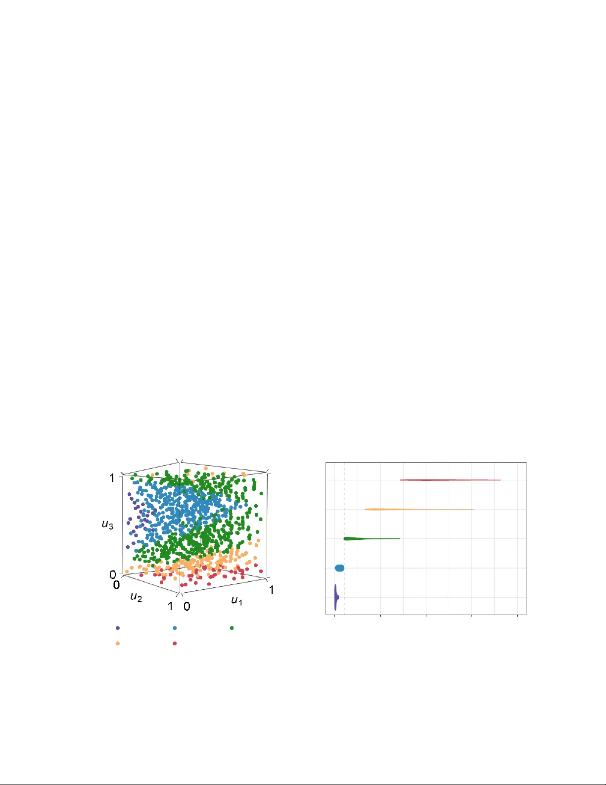
Bio equiv alence Design with Sampling Distribution Segmen ts Luk e Hagar ∗ Nathaniel T. Stev ens Dep artment of Statistics & A ctuarial Scienc e University of Waterlo o, Waterlo o, ON, Canada, N2L 3G1 Abstract In bio equiv alence design, p ow er analyses dictate ho w muc h data must be collected to detect the ab- sence of clinically important eﬀects. Po wer is computed as a tail probability in the sampling distribution of the p ertinen t test statistics. When these test statistics cannot b e constructed from pivotal quan tities, their sampling distributions are approximated via rep etitiv e, time-intensiv e computer simulation. W e prop ose a no v el sim ulation-based metho d to quickly approximate the p o wer curve for man y such bio e- quiv alence tests b y eﬃciently exploring segments (as opp osed to the en tirety) of the relev ant sampling distributions. Despite not estimating the en tire sampling distribution, this approach prompts unbiased sample size recommendations. W e illustrate this method using t wo-group bioequiv alence tests with un- equal v ariances and ov erview its broader applicabilit y in clinical design. All metho ds proposed in this w ork can b e implemented using the developed dent pack age in R. Keyw ords: Average bio equiv alence; p o w er analysis; scalable design; Sob ol’ sequences; W elc h’s t -test 1 In tro duction Bio equiv alence studies require a substantial inv estmen t of time, funding, and h uman capital. It is imp ortant to ensure these resources are inv ested in w ell-designed studies that are capable of achieving their intended ob jectives. Bio equiv alence study ob jectives in volv e establishing the absence of a clinically imp ortan t diﬀer- ence b et ween treatment eﬀects to exp edite the approv al pro cess for reform ulations of existing drugs. The p o w er of a bio equiv alence study is the probability of correctly establishing the absence of such eﬀects ( Cho w and Liu , 2008 ). The study pow er generally increases with the sample size, and a pow er analysis is typically used to ﬁnd the minim um sample size that achiev es the desired p o wer for a study . A p o wer analysis considers the sampling distributions of a relev ant test statistic under tw o hypotheses: the null hypothesis H 0 and alternative hypothesis H 1 . F or bio equiv alence studies, H 0 supp oses that there exists a clinically imp ortant diﬀerence b et ween tw o treatmen ts, and the alternative hypothesis H 1 assumes the absence of suc h a diﬀerence. Under the assumption that H 0 is true, this sampling distribution is called the null distribution. F or most parametric frequentist bio equiv alence te sts, the n ull distribution coincides with a kno wn statistical distribution based on pivotal quantities ( Shao , 2003 ) that do es not dep end on the unkno wn model parameters. In con trast, the sampling distribution of the test statistic under H 1 do es dep end on the magnitude of the eﬀect size, expressed as a function of the mo del parameters. Po w er is deﬁned as a tail ∗ Luke Hagar is the corresp onding author and may b e contacted at lmhagar@uwaterloo.ca . 1 probabilit y in the sampling distribution under H 1 , where the threshold for this tail probability is called the critical v alue. This tail probability is straightforw ard to compute via integration when the n ull distribution is based on a pivotal quan tity , but more complex methods must b e used to perform p o wer analysis otherwise. The null distribution is not based on piv otal quantities for man y bio equiv alence studies, particularly those that leverage the W elch-Satterth waite equation ( Satterthw aite , 1946 ; W elc h , 1947 ) to appro ximate the degrees of freedom for linear combinations of indep enden t sample v ariances. This equation is applied to assess bio equiv alence based on crossov er designs ( Lui , 2016 ), sev eral treatmen ts ( Jan and Shieh , 2020 ), and sequen tial testing ( T artak ovsky et al. , 2015 ). Additionally , the most common application of this equation is to compare t wo normal population means with unequal population v ariances via W elc h’s t -test ( W elc h , 1938 ): the default t -test in the programming language R. Even for this most basic use case, the null distribution is not based on a pivotal quantit y . The null distribution for W elch’s t -test approximately coincides with the standard normal distribution for large sample sizes, but this approximation based on asymptotic pivotal quan tities is of limited utility since t -tests are most useful when the sample sizes are small (e.g., in early phases of clinical trials). This pap er presents a general framew ork for p o wer analysis without the use of pivotal quan tities that is primarily illustrated via t wo-group bio equiv alence tests with unequal v ariances. W e fo cus on this setting for three reasons. First, these tests commonly assess av erage bio equiv alence ( Chow and Liu , 2008 ) of t wo phar- maceutical drugs. Average bio equiv alence compares the me an clinical responses for tw o or more treatments. Second, this setting allo ws for clear visualization of our metho dology . Third, existing metho ds for p o wer analysis with these designs (see e.g., P ASS ( NCSS, LLC. , 2023 )) pro duce unreliable results as demonstrated in this pap er. While this pap er emphasizes t wo-group bio equiv alence tests with unequal v ariances, we later illustrate the use of the prop osed metho ds with crosso ver designs. The metho ds are also generally appli- cable with equiv alence, noninferiority , and one-sided hypothesis tests in nonclinical settings. The metho ds prop osed in this pap er (as well as several extensions) can all b e implemen ted using the dent pack age in R ( Hagar and Stev ens , 2024 ). P ow er analysis requires practitioners to c ho ose anticipated eﬀect sizes and v ariability estimates based on previous studies ( Chow et al. , 2008 ). The recommended sample sizes achiev e desired statistical p o wer when the selected resp onse distributions, an ticipated eﬀect sizes, and v ariabilit y estimates accurately char- acterize the underlying data generation pro cess. Empirical p o wer analysis prompts more ﬂexible metho ds for bio equiv alence study design when the n ull distribution is not based on piv otal quantities. Ho wev er, sim ulation-based methods for pow er analysis hav e computational dra wbac ks. Standard practice requires sim ulating many samples of data to reliably approximate the sampling distribution needed to estimate p o w er for each sample size n considered. This standard practice of estimating entir e sampling distributions of test statistics is w asteful becaus e study p o wer is a tail probability in the sampling distribution under H 1 2 deﬁned by a critical v alue. It would b e more computationally eﬃcient if we could accurately assess p o wer for a sample size n by only exploring a se gment of the sampling distribution that is near the critical v alue. The metho ds for pow er analysis prop osed in this pap er adopt such an approach. The remainder of this article is structured as follows. In Section 2 , we presen t a metho d to map sampling distributions of test statistics for tw o-group bio equiv alence tests with unequal v ariances to the unit cub e. This mapping prompts unbiased p o wer estimates given a pseudorandom or low-discrepancy sequence dis- p ersed throughout the unit cub e. In Section 3 , we prop ose a nov el sim ulation-based metho d that com bines the mapping from Section 2 with ro ot-ﬁnding algorithms to quickly facilitate p ow er curve approximation. This approach is fast b ecause for a given sample size, we only explore test statistics corresp onding to sub- spaces of the unit cub e – and hence only consider a segment of the sampling distribution. Even without estimating entire sampling distributions, we show this metho d yields unbiased sample size recommenda- tions. T o illustrate the wide applicabilit y of the prop osed metho dology , we extend this approac h for use with crosso ver bio equiv alence designs in Section 4 . Throughout the pap er, we also describ e how the metho ds can b e applied with more complex study designs. W e provide concluding remarks and a discussion of extensions to this w ork in Section 5 . 2 Mapping the Sampling Distribution to the Unit Cube 2.1 Three-Dimensional Simulation Rep etitions The results in this section are used to appro ximate p ow er curves with segments of the relev ant sampling distributions in Section 3 . In this section, we describ e ho w to map the sampling distribution of test statis- tics for tw o-group bio equiv alence tests to an appropriate unit hypercub e [0 , 1] w with lo w dimension w . This mapping allo ws us to implemen t pow er analyses without necessitating the high-dimensional simulation asso ci- ated with rep eatedly generating data. W e consider a con text which prompts a three-dimensional simulation corresp onding to the unit cub e for illustration. In particular, w e supp ose w e collect bioa v ailabilit y data y ij , i = 1 , ..., n j , j = 1 , 2 from the i th sub ject in group j . The sub jects in group 1 are assigned to take the new (test) drug formulation, whereas the sub jects in group 2 are assigned to take the established (reference) drug. W e assume for illustration that the data y j = { y ij } n j i =1 for group j = 1 , 2 are generated indep endently from a N ( µ j , σ 2 j ) distribution where σ 2 1  = σ 2 2 . In terest lies in comparing µ 1 and µ 2 while accounting for unequal v ariances. Bio equiv alence limits ( δ L , δ U ) are deﬁned to determine whether diﬀerences b et ween the formulations are clinically imp ortan t. Guidance for choosing clinically imp ortan t diﬀerences is often provided by regulatory b odies, such as the U.S. F o od and Drug Administration (FDA) ( FD A , 2003 , 2022 ). Ho wev er, the metho ds in this section accommo date any real −∞ < δ L < δ U < ∞ . Given bio equiv alence limits δ L and δ U , we aim to conclude that µ 1 − µ 2 ∈ ( δ L , δ U ) to supp ort av erage bio equiv alence of the tw o drug formulations. 3 W e do so by rejecting the comp osite null hypothesis H 0 : µ 1 − µ 2 ∈ ( −∞ , δ L ] ∪ [ δ U , ∞ ) in fa vour of the alternativ e h yp othesis H 1 : µ 1 − µ 2 ∈ ( δ L , δ U ). F or suc h analyses, Sch uirmann ( 1981 ) and Dannen b erg et al. ( 1994 ) resp ectiv ely prop osed tw o one-sided test (TOST) pro cedures based on Studen t’s and W elch’s t -tests, with the W elc h-based TOST pro cedure p erforming b etter than the standard v ersion in the presence of unequal v ariances ( Gruman et al. , 2007 ; Rusticus and Lo v ato , 2014 ). W e henceforth refer to the W elch- based TOST pro cedure as the TOST pro cedure. F or completeness, Bay esian ( Mandallaz and Mau , 1981 ; Ghosh and Rosner , 2007 ; Griev e , 2023 ) and nonparametric ( Hausc hk e et al. , 1990 ; W ellek , 1996 ; Meier , 2010 ) alternativ es to the TOST pro cedure for concluding a verage bioequiv alence also exist, though this is not our fo cus. The TOST pro cedure decomp oses the interv al n ull hypothesis H 0 in to t wo one-sided h yp otheses. These h yp otheses are H 0 L : µ 1 − µ 2 ≤ δ L vs. H 1 L : µ 1 − µ 2 > δ L and H 0 U : µ 1 − µ 2 ≥ δ U vs. H 1 U : µ 1 − µ 2 < δ U . T o conclude µ 1 − µ 2 ∈ ( δ L , δ U ), both H 0 L and H 0 U m ust b e rejected at the nominal level of signiﬁcance α . With W elch’s t -tests, w e therefore require that t L = ( ¯ y 1 − ¯ y 2 ) − δ L p s 2 1 /n 1 + s 2 2 /n 2 ≥ t 1 − α ( ν ) and t U = δ U − ( ¯ y 1 − ¯ y 2 ) p s 2 1 /n 1 + s 2 2 /n 2 ≥ t 1 − α ( ν ) , where s 2 j is the sample v ariance for group j = 1 , 2 and t 1 − α ( ν ) is the upp er α -quantile of the t -distribution with ν degrees of freedom. The degrees of freedom for b oth t -tests are ν =  s 2 1 n 1 + s 2 2 n 2  2 ×  s 4 1 n 2 1 ( n 1 − 1) + s 4 2 n 2 2 ( n 2 − 1)  − 1 . (1) Because ν is a function of the sample v ariances, the null distribution is not based on exact pivotal quan tities. The critical v alue t 1 − α ( ν ) for the test statistics t L and t U therefore dep ends on the data. The data are unknown a priori, whic h complicates an analytical p o wer analysis that uses in tegration. Jan and Shieh ( 2017 ) considered analytical p o wer analysis for the TOST pro cedure with unequal v ariances by expressing the test statistics in terms of simpler normal, chi-square, and b eta random v ariables. Ho wev er, the consistency of their p o wer estimates dep ends on the numerical in tegration settings as demonstrated in Section SM2 of the online supplemen t. W e instead use simulation to obtain consistent pow er estimates. T o compute the test statistics t L and t U , w e need only simulate three sample summary statistics: ¯ y 1 − ¯ y 2 , s 2 1 , and s 2 2 . When the data are indeed generated from the an ticipated N ( µ j , σ 2 j ) distributions, these sample summary statistics are suﬃcien t and can be expressed in terms of kno wn normal and c hi-square distributions. W e generate these summary statistics using three-dimensional (3D) randomized Sob ol’ sequences of length m : u r = ( u 1 r , u 2 r , u 3 r ) ∈ [0 , 1] 3 for r = 1 , ..., m . Sobol’ sequences ( Sob ol’ , 1967 ) are low-discrepancy se- quences based on integer expansion in base 2 that induce negativ e dependence betw een the points U 1 , ..., U m . Sob ol’ sequences are regularly incorp orated into quasi-Monte Carlo metho ds, and they can b e randomized via digital shifts ( Lemieux , 2009 ). W e generate and randomize Sob ol’ sequences in R using the qrng pack age ( Hofert and Lemieux , 2020 ). 4 When using randomized Sob ol’ sequences, each p oin t in the sequence is such that U r ∼ U  [0 , 1] 3  for r = 1 , ..., m . It follo ws that randomized Sobol’ sequences can be used similarly to pseudorandom sequences in Monte Carlo simulation to prompt unbiased estimators: E 1 m m X r =1 Ψ( U r ) ! = Z [0 , 1] 3 Ψ( u ) d u , (2) for some function Ψ( · ). Due to the negative dep endence b et ween the p oin ts, the v ariance of the estimator in ( 2 ) is typically reduced by using low-discrepancy sequences. W e hav e that V ar 1 m m X r =1 Ψ( U r ) ! = V ar (Ψ( U r )) m + 2 m 2 m X r =1 m X t = r +1 Co v (Ψ( U r ) , Ψ( U t )) , (3) where the the ﬁrst term on the right side of ( 3 ) is the v ariance of the corresp onding estimator based on pseudorandom sequences of indep enden tly generated p oin ts. While underutilized in simulation-based study design, low-discrepancy sequences give rise to eﬀective v ariance reduction metho ds when the dimension of the sim ulation is m oderate. W e can therefore use fewer simulation rep etitions m to obtain unbiased p ow er estimates with Sob ol’ sequences in lieu of pseudorandom alternatives. Algorithm 1 outlines our pro cedure for unbiased empirical p o wer estimation at sample sizes n 1 and n 2 using a Sob ol’ sequence of length m and signiﬁcance level α for each t -test. F or each of the m p oin ts from the 3D Sob ol’ sequence, we obtain v alues for the summary statistics ¯ y 1 − ¯ y 2 , s 2 1 , and s 2 2 using cumulativ e distribution function (CDF) inv ersion. W e let F ( · ; ν ) and Φ − 1 ( · ) b e the inv erse CDFs of the χ 2 ( ν ) and standard normal distributions, resp ectiv ely . Given these summary statistics, we determine whether the sample for a giv en sim ulation repetition corresp onds to the bioequiv alence test’s rejection region. The proportion of the m Sob ol’ sequence p oin ts for which this o ccurs estimates the p ow er of the test. The test statistic for each t -test is comprised of tw o random comp onents: (1) ¯ d = ¯ y 1 − ¯ y 2 in the n umerator and (2) se = p s 2 1 /n 1 + s 2 2 /n 2 in the denominator. The rejection region for the TOST pro cedure is a triangle in the ( ¯ d, se )-space with v ertices ( δ L , 0), ( δ U , 0), and (0 . 5 ( δ L + δ U ) , 0 . 5 ( δ U − δ L ) /t 1 − α ( ν )). The pro cedure in Algorithm 1 along with this rejection region is visualized in Figure 1 . Algorithm 1 Pro cedure to Compute Empirical Po wer 1: pro cedure EmpiricalPower ( µ 1 − µ 2 , σ 1 , σ 2 , δ L , δ U , α, n 1 , n 2 , m ) 2: reject ← null 3: Generate a Sobo l’ sequence of length m : u r = ( u 1 r , u 2 r , u 3 r ) ∈ [0 , 1] 3 for r = 1 , ..., m . 4: for r in 1: m do 5: Let s 2 j r = ( n j − 1) − 1 σ 2 j F ( u j r ; n j − 1) for j = 1 , 2 6: Let ¯ d r = ( µ 1 − µ 2 ) + Φ − 1 ( u 3 r ) p σ 2 1 /n 1 + σ 2 2 /n 2 7: Use s 2 1 r and s 2 2 r to compute se r and ν r via ( 1 ) 8: reject [w] ← ifelse( t 1 − α ( ν r ) se r < min { ¯ d r − δ L , δ U − ¯ d r } , 1, 0) 9: return mean(reject) as empirical pow er T o apply this approach with more complex (bio equiv alence) study designs, sampling distributions for h yp othesis tests can b e mapp ed to [0 , 1] w , where w is the num b er of suﬃcient statistics required to compute 5 s 1 s 2 d 0 δ U − δ L 2t 1 −α ( ν ) δ L δ U d s e Figure 1: Left: Example p oin t (0 . 785 , 0 . 009 , 0 . 694) ∈ [0 , 1] 3 . Cen ter: Mapping from this p oin t to suﬃcient statistics. Right: The rejection region for the TOST pro cedure. the relev ant test statistics. T o design Ba y esian p osterior analyses, Hagar and Stev ens ( 2023 ) leveraged maxim um lik eliho o d estimates when low-dimensional suﬃcien t statistics did not exist or w ere diﬃcult to generate. Those metho ds rely on large-sample results but could b e applied in frequen tist settings. The sim ulation dimension w may b e large if using these mappings to design sequen tial tests with many interim analyses or facilitate extensive m ulti-group comparisons. If w ≥ 32, caution should b e exercised when using quasi-Mon te Carlo metho ds; high-dimensional low-discrepancy sequences may ha ve p o or low-dimensional pro jections, whic h can lead to a deterioration in p erformance ( Lemieux , 2009 ). Pseudorandom sequences could instead be used to implement such large-dimensional mappings. F or tw o-group bio equiv alence tests, p o wer analysis could b e implemented by estimating p o wer via Algo- rithm 1 at v arious sample sizes un til the desired study p o wer of 1 − β is achiev ed for some type I I error rate β . Ho wev er, that approach w ould b e ineﬃcien t since we w ould need to thoroughly explore [0 , 1] 3 – and hence consider the en tire sampling distribution – at each com bination of sample sizes considered. Low-discrepancy sequences already allow us to obtain precise p o wer estimates using fewer p oin ts from [0 , 1] 3 than pseudo- random sequences. W e can further improv e this eﬃciency by only exploring subspaces of [0 , 1] 3 that help us estimate p o wer. W e develop a metho dology for this in Section 3 . But ﬁrst, we introduce a motiv ating example that will b e used to assess the p erformance of our metho d for p o wer curve approximation prop osed later. W e illustrate the use of Algorithm 1 in this context. 2.2 Motiv ating Example This motiv ating example is adapted from P ASS 2023 do cumen tation ( NCSS, LLC. , 2023 ). P ASS is a paid soft ware solution that facilitates p o wer analysis and sample size calculations for tw o-group (bio)equiv alence tests with unequal v ariances. The motiv ating example is represen tative of a standard tw o-group bioequiv a- 6 Estimated Po wer n P AS S Alg 1 Na ¨ ıv e Sim ulation 3 0.1073 0.0414 (1 . 43 × 10 − 4 ) 0.0414 (7 . 85 × 10 − 4 ) 5 0.1778 0.1283 (1 . 70 × 10 − 4 ) 0.1282 (1 . 27 × 10 − 3 ) 8 0.4094 0.3801 (2 . 60 × 10 − 4 ) 0.3800 (2 . 03 × 10 − 3 ) 10 0.5527 0.5366 (2 . 68 × 10 − 4 ) 0.5368 (2 . 03 × 10 − 3 ) 15 0.7723 0.7699 (1 . 49 × 10 − 4 ) 0.7700 (1 . 88 × 10 − 3 ) 20 0.8810 0.8815 (1 . 65 × 10 − 4 ) 0.8816 (1 . 39 × 10 − 3 ) 30 0.9679 0.9687 (9 . 32 × 10 − 5 ) 0.9688 (6 . 66 × 10 − 4 ) 40 0.9924 0.9922 (5 . 28 × 10 − 5 ) 0.9922 (3 . 24 × 10 − 4 ) 50 0.9982 0.9982 (3 . 45 × 10 − 5 ) 0.9982 (1 . 67 × 10 − 4 ) 60 0.9996 0.9996 (2 . 10 × 10 − 5 ) 0.9996 (7 . 22 × 10 − 5 ) T able 1: P ow er estimates presen ted in the P AS S do cumen tation along with the mean of 100 empirical p o w er estimates obtained via Algorithm 1 (Alg 1) and simulating normal data (Na ¨ ıve Sim ulation). Standard deviations of the 100 empirical p o wer estimates are giv en in parentheses. lence design and seeks to compare the impact of t wo drugs on diastolic bloo d pressure, measured in mmHg (millimeters of mercury). The mean diastolic blo od pressure is known to b e roughly µ 2 = 96 mmHg with the reference drug ( j = 2), and it is hypothesized to b e ab out µ 1 = 92 mmHg with the test drug ( j = 1). Sub ject matter exp erts use past studies to hypothesize within-group diastolic blo od pressure standard de- viations of σ 1 = 18 mmHg and σ 2 = 15 mmHg, resp ectively . The bio equiv alence limits for the study are δ U = 0 . 2 × 96 = 19 . 2 and δ L = − δ U to comply with the FDA’s ± 20 rule ( FD A , 2006 ). The signiﬁcance level for the test is α = 0 . 05. The P ASS documentation considers p o wer for the motiv ating example at n = n 1 = n 2 = { 3 , 5 , 8 , 10 , 15 , 20 , 30 , 40 , 50 , 60 } . F or eac h sample size n , we estimated p ow er 100 times using Algorithm 1 with m = 2 16 = 65536. W e also obtained 100 empirical p ow er estimates for each sample size n by generating m samples of size n from the N ( µ 1 , σ 2 1 ) and N ( µ 2 , σ 2 2 ) distributions and recording the prop ortion of samples for which w e concluded that µ 1 − µ 2 ∈ ( δ L , δ U ). T able 1 summarizes these n umerical results and the p o wer estimates presen ted in the P ASS do cumentation. In recognition of their licensing agreemen t, P ASS soft ware was not used nor accessed to conﬁrm these p ow er estimates. The tw o simulation-based approaches provide unbiased p ow er estimates. How ever, T able 1 sho ws that the p o w er estimates obtained via Algorithm 1 are m uch more precise than those obtained via na ¨ ıv e simulation with pseudorandom sequences. Moreo ver, eac h p o wer estimate was obtained in roughly a quarter of a second when using Algorithm 1 . It to ok b et ween 20 and 30 seconds to obtain each p o wer estimate using na ¨ ıv e sim ulation. This o ccurs b ecause – regardless of the sample size n considered – Algorithm 1 reduces the p ow er calculation to a three-dimensional problem that can b e eﬃciently v ectorized. W e must use for lo ops to estimate p o wer when directly generating the higher-dimensional data y 1 and y 2 . Moreo v er, the p o w er estimates presented in the P ASS documentation do not coincide with those returned via simulation for sample sizes less than 15, suggesting that it is v aluable to develop more accurate metho ds for p o w er 7 analysis with bioequiv alence designs. 3 P o w er Curv e Appro ximation with Segmen ts of the Sampling Distribution 3.1 An Eﬃcient Approach to P ow er Analysis In this section, we leverage the mapping betw een the unit cub e and the test statistics presented in Section 2 to facilitate p o wer curve approximation while estimating only segments of the sampling distribution. F or giv en sample sizes n 1 and n 2 , we previously mapp ed each Sob ol’ sequence p oin t u r ( r = 1 , ..., m ) to a mean diﬀerence, standard error, and degrees of freedom for its test statistic: ¯ d r , se r , and ν r . T o compute empirical p o w er in Algorithm 1 , we ﬁxed the sample sizes n 1 and n 2 and allow ed the Sob ol’ sequence p oin t to v ary . W e no w sp ecify a constant q > 0 such that n = n 1 = q n 2 to allow for imbalanced sample sizes. When appro ximating the p o wer curve, we ﬁx the Sobol’ sequence p oin t u r and let the sample size n v ary . W e in tro duce the notation ¯ d ( n,q ) r , se ( n,q ) r , and ν ( n,q ) r to mak e this clear. F or ﬁxed q and r , these quan tities are only functions of the sample size n . As n → ∞ , ¯ d ( n,q ) r , se ( n,q ) r , and ν ( n,q ) r approac h µ 1 − µ 2 , 0, and ∞ , resp ectiv ely . W e consider the b eha viour of these functions when H 1 is true, i.e., when µ 1 − µ 2 ∈ ( δ L , δ U ). The upper v ertex of the triangular rejection region for the TOST procedure is  0 . 5( δ L + δ U ) , 0 . 5 ( δ U − δ L ) /t 1 − α ( ν ( n,q ) r )  . First, ν ( n,q ) r almost alwa ys increases for ﬁxed r and q as n increases. Th us as n → ∞ , the vertical co ordinate of this rejection region vertex increases to 0 . 5 ( δ U − δ L ) / Φ − 1 (1 − α ), and the remaining tw o v ertices do not c hange. The rejection region then deﬁnes a threshold for the standard error se ( n,q ) r : Λ ( n,q ) r = min { ¯ d ( n,q ) r − δ L , δ U − ¯ d ( n,q ) r } /t 1 − α ( ν ( n,q ) r ). W e conclude µ 1 − µ 2 ∈ ( δ L , δ U ) if and only if se ( n,q ) r do es not exceed this threshold. F or ﬁxed r and q , this threshold is also a function of n : Λ ( n,q ) r :=                ( µ 1 − µ 2 ) − δ L t 1 − α ( ν ( n,q ) r ) + Φ − 1 ( u 3 r ) p σ 2 1 + σ 2 2 /q √ nt 1 − α ( ν ( n,q ) r ) if δ L < ¯ d ( n,q ) r ≤ 0 . 5( δ L + δ U ) δ U − ( µ 1 − µ 2 ) t 1 − α ( ν ( n,q ) r ) − Φ − 1 ( u 3 r ) p σ 2 1 + σ 2 2 /q √ nt 1 − α ( ν ( n,q ) r ) if 0 . 5 ( δ L + δ U ) < ¯ d ( n,q ) r < δ U 0 otherwise. (4) W e supp ose that a given p oin t u r yields se ( n,q ) r ≤ Λ ( n,q ) r , which corresp onds to the rejection region of the TOST pro cedure. In Appendix A , we discuss wh y se ( n +1 ,q ) r ≤ Λ ( n +1 ,q ) r generally also holds true for the same p oin t u r . In light of this, our metho d to approximate the p o wer curve generates a single Sob ol’ sequence of length m . W e use ro ot-ﬁnding algorithms ( Brent , 1973 ) to ﬁnd the smallest v alue of n such that se ( n,q ) r ≤ Λ ( n,q ) r for eac h p oin t r = 1 , ..., m . W e then use the empirical CDF of these m sample sizes to appro ximate the p o wer curve as describ ed in Algorithm 2 . W e now elab orate on several of the steps in Algorithm 2 . Lines 2 to 6 describ e a pro cess that would yield an unbiased p o wer curv e and sample size recommendation if se ( n,q ) r = Λ ( n,q ) r w ere guaranteed to hav e a unique solution in terms of n for ﬁxed r and q . How ever, se ( n,q ) r and Λ ( n,q ) r ma y infrequently in tersect 8 Algorithm 2 Pro cedure for Po wer Curve Approximation 1: pro cedure PowerCur ve ( µ 1 − µ 2 , σ 1 , σ 2 , δ L , δ U , α , β , q , m ) 2: sampSobol ← null 3: for r in 1: m do 4: Generate Sob ol’ sequence point u r 5: Let sampSobol [ r ] solve se ( n,q ) r − Λ ( n,q ) r = 0 in terms of n 6: Let n ∗ b e the (1 − β )-quan tile of sampSobol 7: for r in 1: m do 8: if sampSobol [ r ] ≤ n ∗ then 9: if se ( n,q ) r > Λ ( n,q ) r then 10: Rep eat Line 5, initializing the root-ﬁnding algorithm at n ∗ 11: else 12: if se ( n,q ) r ≤ Λ ( n,q ) r then 13: Rep eat Line 5, initializing the root-ﬁnding algorithm at n ∗ 14: powerCurve ← empirical CDF of sampSobol 15: Let n ∗ b e the (1 − β )-quan tile of sampSobol 16: return powerCurve , n 1 = ⌈ n ∗ ⌉ and n 2 = ⌈ q n ∗ ⌉ as the recommended sample sizes more than once. Given the reasoning in App endix A and the numerical studies in Section SM1 of the online supplemen t, these multiple intersections do not o ccur frequently enough to deter us from using ro ot-ﬁnding algorithms to explore sample sizes. With ro ot-ﬁnding algorithms, we explore only subspaces of [0 , 1] 3 for eac h sample size inv estigated since diﬀerent v alues of n are considered for eac h p oint u r in Line 4. Ro ot- ﬁnding algorithms therefore give rise to computational eﬃciency as the entire sampling distribution is not estimated when exploring sample sizes n . In particular, the ro ot-ﬁnding algorithm computes test statistics corresp onding to O (log 2 B ) p oin ts from [0 , 1] 3 , where B is the maxim um sample size considered for the pow er curv e. W e w ould require O ( B ) such p oin ts to explore a similar range of sample sizes using p ow er estimates from Algorithm 1 . When B ≥ 59, this approac h reduces the num b er of test statistics we must estimate b y at least an order of magnitude b ecause O (log 2 B ) < O ( B ) / 10. Using lo w-discrepancy sequences instead of pseudorandom ones further reduces the num b er of test statistics we must estimate as demonstrated in Section 3.2 . If we skipp ed Lines 7 to 14 of Algorithm 2 , the unbiasedness of the sample size recommendation in Line 16 is not guaranteed due to the p oten tial for multiple intersections b etw een se ( n,q ) r and Λ ( n,q ) r . T o ensure our sample size recommendations are unbiased despite using subspaces of [0 , 1] 3 to consider sample sizes, we estimate the en tire sampling distribution of test statistics at the sample size n = n ∗ in Lines 7 to 13. If the statemen ts in Lines 9 or 12 are true, this implies that se ( n,q ) r = Λ ( n,q ) r for at least tw o distinct sample sizes n . F or these points u r , w e can reinitialize the ro ot-ﬁnding algorithm at n ∗ to obtain a solution for eac h p oin t that will make the p o wer curve unbiased at n ∗ . Our numerical studies in Section 3.2 show that the if statemen ts in Lines 9 and 12 are very rarely true for any point u r ∈ [0 , 1] 3 . In those situations, n ∗ = n ∗ and b oth the p o wer estimate at n ∗ and the sample size recommendations ⌈ n ∗ ⌉ and ⌈ q n ∗ ⌉ are unbiased. It is incredibly unlik ely that n ∗ and n ∗ w ould diﬀer substantially , but Lines 7 to 13 of Algorithm 2 could 9 b e rep eated in that even t, where the ro ot-ﬁnding algorithm is initialized at n ∗ instead of n ∗ . Even when se ( n,q ) r and Λ ( n,q ) r in tersect more than once, the p o wer curves from Algorithm 2 are unbiased near the target p o w er 1 − β , but their global unbiasedness at all sample sizes n is not strictly guaranteed. Nevertheless, our n umerical studies in Section 3.2 highligh t goo d global estimation of the p o wer curve. The metho ds we lev eraged to select subspaces of [0 , 1] 3 for tw o-group bio equiv alence tests are tailored to the functions se ( n,q ) r and Λ ( n,q ) r . How ever, these metho ds rely more generally on the weak law of large n umbers since most suﬃcien t statistics are based on sample means. Up on mapping the unit h yp ercube [0 , 1] w to suﬃcien t statistics, the b eha viour of the test statistics as a function of the sample size n can generally b e studied to dev elop analogs to Algorithm 2 for other tests and designs. Ro ot-ﬁnding algorithms are generally useful when the rejection region is conv ex. Rejection regions for the TOST pro cedure in Figure 1 , other (bio)equiv alence tests, and one-sided h yp othesis tests are t ypically con vex, whereas hypothesis tests with p oin t null hypotheses often ha ve non-conv ex rejection regions. 3.2 Numerical Study with the Motiv ating Example W e reconsider the motiv ating example from Section 2.2 to illustrate the reliable p erformance of our eﬃcient metho d for p o wer curve approximation. F or this example, we approximate the p o wer curve 1000 times with q = 1 (i.e., n = n 1 = n 2 ). Each of the 1000 p o wer curves are appro ximated using Algorithm 2 with a target p ow er of 1 − β = 0 . 8 and a Sob ol’ sequence of length m = 2 10 = 1024. W e recommend using shorter Sob ol’ sequences when appro ximating the p o w er curve than when computing empirical p o wer for a sp eciﬁc ( n 1 , n 2 ) combination ( m = 65536 w as used in Section 2.2 ). Whereas all computations in Algorithm 1 can b e v ectorized, w e must use a for lo op to implement the root-ﬁnding algorithm for eac h Sob ol’ sequence p oin t. W e compare these 1000 p o wer curves to the un biased p o wer estimates from Algorithm 1 in T able 1 . The left plot of Figure 2 demonstrates that Algorithm 2 yields suitable global p o wer curve approximation when comparing its results to these p o wer estimates. Eac h p o wer curve was approximated without estimating the entire sampling distribution for all sample sizes n 1 and n 2 explored as emphasized in Section 3.3 . T o further inv estigate the p erformance of Algorithm 2 , we rep eated the pro cess from the previous paragraph to estimate 1000 p ow er curves for the motiv ating example with 1 − β = { 0 . 2 , 0 . 3 , . . . , 0 . 7 , 0 . 9 } . In total, we appro ximated 8000 p o wer curves for this example. Using the ro ot-ﬁnding algorithm to explore the sample size space did not lead to p erformance issues. W e did not need to reinitialize the ro ot-ﬁnding algorithm in Lines 7 to 13 of Algorithm 2 for any of the 8 . 192 × 10 6 p oin ts used to generate these 8000 curves. The suitable p erformance of Algorithm 2 is corrob orated b y more extensiv e n umerical studies detailed in Section SM1 of the online supplement. T o assess the impact of using Sob ol’ sequences with Algorithm 2 , w e approximated 1000 p o wer curv es for the motiv ating example using ro ot-ﬁnding algorithms with 1 − β = 0 . 8 and sequences from a pseudorandom n umber generator. W e then used the 1000 p o wer curves corresp onding to each sequence type (Sob ol’ and 10 0.00 0.25 0.50 0.75 1.00 0 20 40 60 n P ow er −0.04 −0.02 0.00 0.02 0.04 20 40 60 n Centered 95% Confidence Inter v al Sobol' PRNG Long PRNG Figure 2: Left: 1000 p o wer curv es estimated for the motiv ating example (gray) and the p o wer estimates obtained via Algorithm 1 (red). Right: Endp oin ts of the cen tered 95% conﬁdence in terv als for pow er obtained with Sob ol’ ( m = 1024) and pseudorandom (PRNG) sequences ( m = 1024 , 10 4 ). pseudorandom) to estimate p o wer for the sample sizes considered in Section 2.2 : n = { 3 , 5 , 8 , 10 , 15 , 20 , 30 , 40 , 50 , 60 } . F or eac h sample size and sequence type, we obtained a 95% conﬁdence interv al for p o wer using the p ercen tile b ootstrap metho d ( Efron , 1982 ). W e then created centered conﬁdence interv als by subtracting the p o w er estimates pro duced by Algorithm 1 from each conﬁdence in terv al endpoint. The right plot of Figure 2 depicts these results for the 10 sample sizes n and tw o sequence types considered. Figure 2 illustrates that the Sob ol’ sequence gives rise to muc h more precise p o wer estimates than pseudorandom sequences – particularly when p ow er is not near 0 or 1. W e rep eated this pro cess to generate 1000 p o wer curv es via Algorithm 2 with pseudorandom sequences of length m = 10 4 . The p o wer estimates obtained using Sob ol’ sequences with length m = 1024 are roughly as precise as those obtained with pseudorandom sequences of length m = 10 4 . Using Sob ol’ sequences therefore allows us to estimate p o wer with the same precision using appro ximately an order of magnitude fewer poin ts from [0 , 1] 3 . Each pow er curve for this example with m = 1024 took just under one second to appro ximate. It would tak e roughly 10 times as long to appro ximate the p o wer curve with the same precision using pseudorandom p oin ts in lieu of Sob ol’ sequences. 3.3 Exploring Subspaces of the Unit Cub e Here, w e demonstrate how segmen ts of the sampling distribution are leveraged when exploring only subspaces of the unit cub e [0 , 1] 3 for most sample sizes considered. The left plot of Figure 3 decomp oses the results of the ro ot-ﬁnding algorithm for one approximated p o wer curve from Section 3.2 with 1 − β = 0 . 8 for the motiv ating example. Even when the root-ﬁnding algorithm is initialized at the same sample size for all { u r } m r =1 , diﬀerent n are considered for each p oin t u r when determining the solution to se ( n,q ) r = Λ ( n,q ) r . The v alue of n is noninteger in most iterations of the ro ot-ﬁnding algorithm, and the colors in the left plot of 11 Figure 3 indicate which p oin ts from the unit cub e w ere considered for v arious ranges of n . F or instance, the purple p oin ts were such that their test statistics corresp onded to the rejection region for the smallest p ossible sample size of n = 2. Moreov er, only the blue p oin ts in [0 , 1] 3 w ere used to estimate test statistics for at least one sample size n ∈ (2 , 8) when exploring v alues of n via the root-ﬁnding pro cedure. The p oin ts that were used to explore the smallest sample sizes generally hav e mo derate u 3 r v alues and smaller u 1 r and u 2 r v alues. The mean diﬀerence ¯ d ( n,q ) r is therefore small in absolute v alue and the sample v ariances for groups 1 and 2 are small, which implies that the numerators of the test statistics t L and t U are large and their denominators are small. The p oin ts used to explore larger sample sizes generally hav e more extreme u 3 r v alues, so ¯ d ( n,q ) r ma y not substan tially diﬀer from one of δ L or δ U for small sample sizes. While the pattern in the left plot of Figure 3 depends on the inputs for Algorithm 2 , the root-ﬁnding algorithm correctly iden tiﬁes which subspaces of [0 , 1] 3 to prioritize for a given sample size n with an arbitrary bio equiv alence design. Our metho ds can b e extended to more complex designs, but it is diﬃcult to visualize the prioritized subspaces of the unit h yp ercube when the sim ulation dimension w is greater than 3. The righ t plot of Figure 3 visualizes the sampling distribution of p -v alues for n = n 1 = n 2 = 8 conditional on the categorizations from the left plot. F or the TOST pro cedure, the p -v alue is the maximum of the p - v alues corresp onding to t L and t U . This p -v alue do es not exceed the signiﬁcance lev el α if and only if se ( n,q ) r ≤ Λ ( n,q ) r . This plot demonstrates why it is w asteful to use the purple p oin ts to consider n ≈ 8 b ecause those p oin ts satisfy se ( n,q ) r ≤ Λ ( n,q ) r for n = 2. It follo ws from App endix A that se ( n,q ) r ≤ Λ ( n,q ) r generally holds true for n ≈ 8 with those p oin ts, and the corresp onding p -v alues are hence smaller than α = 0 . 05. By n 2 (2, 8) (8, 16) (16, 26) (26, 60) 0.00 0.25 0.50 0.75 1.00 p −value ( n = 8) Figure 3: Left: Visualization of which p oin ts in [0 , 1] 3 w ere used to explore at least one n v alue in the v arious sample size ranges via the ro ot-ﬁnding algorithm. Right: Violin plots for the sampling distribution of p -v alues corresp onding to n = 8 conditional on the colored categorization of p oin ts. The dotted vertical line is at α = 0 . 05. 12 similar logic, it is w asteful to consider the red p oin ts for n ≈ 8 since the p -v alues for those p oin ts will b e m uch larger than α . Although these colored categorizations are not used in Algorithm 2 , they illustrate the targeted nature of how w e consider sample sizes n with segments of the relev an t sampling distributions. 4 Eﬃcien t Po w er Analysis for Crosso ver Designs The method for pow er curv e approximation in Algorithm 2 w as tailored to a standard parallel bio equiv alence study with unequal v ariances. How ev er, the underlying ideas generalize to other study designs. In particular, w e describe here how to extend Algorithm 2 for use with crossov er designs. Po wer analysis for crossov er designs is of particular in terest because regulatory agencies often recommend using them to conclude a verage bio equiv alence ( FDA , 2006 ). In crossov er designs, eac h sub ject receiv es more than one formulation of a drug during diﬀerent p eriods ( Chow and Liu , 2008 ). This is adv an tageous in that in ter-sub ject v ariability is remov ed from b et ween-form ulation comparisons. W e describ e how to use our design metho ds based on sampling distribution segmen ts with tw o-sequence, tw o-p eriod crossov er designs in Section SM3 of the online supplemen t. W e also highlight discrepancies (of up to 33%) b et ween the sample sizes recommended b y the p o w er curves from Algorithm 2 and those endorsed in p opular textb ooks on bio equiv alence study design ( Cho w and Liu , 2008 ). The implemen tation of suc h extensions for these and other crosso v er designs is supp orted in the dent pac k age developed in conjunction with this paper. F urthermore, our metho d for p o w er analysis is ﬂexible and could readily accommo date additional (bio equiv alence) designs not discussed in this article. 5 Discussion In this pap er, we developed a framework for p o wer analysis that estimates p o wer curves using sampling distribution segments. Our prop osed metho ds are useful when the relev ant test statistics are not based on exact piv otal quantities, which is the case for v arious bioe quiv alence designs. This framework for p o wer analysis maps the unit hypercub e [0 , 1] w to suﬃcient statistics and lev erages this mapping to select sampling distribution segmen ts. Using segmen ts of sampling distributions improv es the scalability of our simulation- based design pro cedures without compromising the unbiasedness of the sample size recommendations. Our framew ork is predominantly illustrated with three-dimensional sim ulation for tw o-group bio equiv alence tests with unequal v ariances, but we describ ed how to apply our metho ds more generally throughout the pap er and now elab orate on several additional extensions. F uture work could apply the framework prop osed in this pap er to design bio equiv alence studies that compare more than tw o form ulations. F or suc h designs, the sim ulation dimension w w ould need to be increased, and the multiple comparisons problem would need to b e considered. It would also b e imp ortan t to extend this design framework to accommo date sequen tial analyses that allow for early termination of the 13 (bio equiv alence) study . Sequential designs consider the o verall p ow er to reject H 0 across all analyses: interim or ﬁnal. T o obtain ov erall p o wer, we require the joint sampling distribution of the test statistics across all analyses to aggregate their marginal p o wers. In sequential settings, w e w ould lik ely need to deﬁne analogues to se ( n,q ) r and Λ ( n,q ) r for each interim analysis and synthesize the results for each p oin t u r . Ho wev er, it is not trivial to create a mapping betw een points in [0 , 1] w and suﬃcien t statistics that main tain the desired level of dep endence b et ween interim analyses for arbitrary sample sizes. Since the design of sequen tial tests requires that w e consider sampling distributions for each planned analysis, the computational sa vings asso ciated with using sampling distribution segments w ould b e comp ounded in these settings. Finally , we could explore ho w this framew ork migh t b e applied to quic kly and reliably recommend sample sizes for nonparametric bio equiv alence testing metho ds ( Meier , 2010 ). The exact null distributions for those tests are not based on pivotal quantities, and it is not p ossible to generate suﬃcient statistics in nonparametric settings. Sample size determination for these studies typically utilizes na ¨ ıve simulation. In nonparametric settings, we may b e able to map the unit hypercub e [0 , 1] w to insuﬃcient statistics, such as sample totals, and use lo w-discrepancy sequences to impro ve the scalability and precision of empirical p o w er analysis. Supplemen tary Material These materials detail additional numerical studies, discussion of comp eting approac hes for p o wer analysis, and considerations for crossov er designs referred to in the pap er. The co de to conduct the numerical studies in the paper is av ailable online: https://github.com/lmhagar/BioDesignSegments . F unding Ac knowledgemen t This work was supp orted by the Natural Sciences and Engineering Research Council of Canada (NSERC) b y w ay of a PGS D sc holarship as well as Grant RGPIN-2019-04212. References Bren t, R. P . (1973). An algorithm with guaranteed con vergence for ﬁnding the minimum of a function of one v ariable. A lgorithms for Minimization without Derivatives, Pr entic e-Hal l, Englewo o d Cliﬀs, NJ , 61–80. Cho w, S. C. and J. P . Liu (2008). Design and A nalysis of Bio availability and Bio e quivalenc e Studies . Chapman and Hall/CRC. Cho w, S. C., J. Shao, and H. W ang (2008). Sample size c alculations in clinic al r ese ar ch . Chapman & Hall/CR C. Dannen b erg, O., H. Dette, and A. Munk (1994). An extension of Welch’s appro ximate t -solution to com- parativ e bio equiv alence trials. Biometrika 81 (1), 91–101. 14 Efron, B. (1982). The jackknife, the b o otstr ap and other r esampling plans . SIAM. FD A (2003). Guidance on bioav ailability and bio equiv alence studies for orally administered drug pro ducts — General considerations. Center for Drug Ev aluation and Researc h, U.S. F oo d and Drug Administration, Ro c kville, MD. FD A (2006). Guidance for industry - Bio equiv alence guidance. Center for Drug Ev aluation and Researc h, U.S. F o o d and Drug Administration, Ro c kville, MD. FD A (2022). Bioav ailabilit y studies submitted in ND As or INDs — General considerations. Center for Drug Ev aluation and Research, U.S. F o od and Drug Administration, Ro c kville, MD. Fisher, R. A. (1934). Statistic al metho ds for r ese ar ch workers (5th ed.). Oliver and Boyd, Edinburgh and London. Ghosh, P . and G. L. Rosner (2007). A semi-parametric Ba yesian approac h to a verage bio equiv alence. Statis- tics in Me dicine 26 (6), 1224–1236. Griev e, A. P . (2023). On implementing Jeﬀreys’ substitution likelihoo d for Bay esian inference concerning the medians of unknown distributions. Pharmac eutic al Statistics 22 (2), 365–377. Gruman, J. A., R. Cribbie, and C. A. Arpin-Cribbie (2007). The eﬀects of heteroscedasticity on tests of equiv alence. Journal of Mo dern Applie d Statistic al Metho ds 6 (1), 133–140. Hagar, L. and N. T. Stev ens (2023). F ast p o wer curve approximation for p osterior analyses. https://arxiv. org/abs/2310.12427 . Hagar, L. and N. T. Stev ens (2024). dent: Design of equiv alence and noninferiorit y tests. R pack age version 0.0.1. https://github.com/lmhagar/dent . Hausc hke, D., V. W. Steinijans, and E. Diletti (1990). A distribution-free pro cedure for the statistical analysis of bioequiv alence studies. International Journal of Clinic al Pharmac olo gy, Ther apy, and T oxic olo gy 28 (2), 72–78. Hofert, M. and C. Lemieux (2020). qrng: (R andomize d) Quasi-R andom Numb er Gener ators . R pack age v ersion 0.0-8. Jan, S.-L. and G. Shieh (2017). Optimal sample size determinations for the heteroscedastic tw o one-sided tests of mean equiv alence: Design schemes and softw are implementations. Journal of Educ ational and Behavior al Statistics 42 (2), 145–165. Jan, S.-L. and G. Shieh (2020). On the extended Welch test for assessing equiv alence of standardized means. Statistics in Biopharmac eutic al R ese ar ch 12 (3), 344–351. 15 Lemieux, C. (2009). Using quasi–monte carlo in practice. In Monte Carlo and Quasi-Monte Carlo Sampling , pp. 1–46. Springer. Lui, K.-J. (2016). Cr ossover Designs: T esting, Estimation, and Sample Size . John Wiley & Sons. Mandallaz, D. and J. Mau (1981). Comparison of diﬀerent metho ds for decision-making in bio equiv alence assessmen t. Biometrics 37 (2), 213–222. Meier, U. (2010). Nonparametric equiv alence testing with resp ect to the median diﬀerence. Pharmac eutic al Statistics 9 (2), 142–150. NCSS, LLC. (2023). Chapter 529 - Tw o-sample t -tests for equiv alence allowing unequal v ariance. Power Anal- ysis and Sample Size (P ASS) 2023 Do cumentation . https://www.ncss.com/wp- content/themes/ncss/ pdf/Procedures/PASS/Two- Sample_T- Tests_for_Equivalence_Allowing_Unequal_Variance.pdf . Rusticus, S. A. and C. Y. Lo v ato (2014). Impact of sample size and v ariability on the p ow er and type i error rates of equiv alence tests: A simulation study . Pr actic al Assessment, R ese ar ch, and Evaluation 19 (1), 11. Satterth waite, F. E. (1946). An approximate distribution of estimates of v ariance comp onents. Biometrics bul letin 2 (6), 110–114. Sc huirmann, D. J. (1981). On hypothesis-testing to determine if the mean of a normal-distribution is con tained in a kno wn in terv al [abstract]. Biometrics 37 (3), 617. Shao, J. (2003). Mathematic al statistics . Springer Science & Business Media. Sob ol’, I. M. (1967). On the distribution of p oints in a cub e and the approximate ev aluation of integrals. Zhurnal Vychislitel’noi Matematiki i Matematicheskoi Fiziki 7 (4), 784–802. T artako vsky , A., I. Nikiforov, and M. Basseville (2015). Se quential A nalysis: Hyp othesis T esting and Change- p oint Dete ction . CRC press. W elch, B. L. (1938). The signiﬁcance of the diﬀerence b et ween tw o means when the p opulation v ariances are unequal. Biometrika 29 (3/4), 350–362. W elch, B. L. (1947). The generalization of ‘Student’s’ problem when several diﬀerent population v arlances are inv olved. Biometrika 34 (1-2), 28–35. W ellek, S. (1996). A new approach to equiv alence assessmen t in standard comparative bioav ailability trials b y means of the Mann-Whitney statistic. Biometric al Journal 38 (6), 695–710. 16 A Justiﬁcation for Using Ro ot-Finding Algorithms Here, we discuss why using ro ot-ﬁnding algorithms to appro ximate the p ow er curve yields suitable results – ev en though se ( n,q ) r and Λ ( n,q ) r can (although infrequently) in tersect more than once. The threshold Λ ( n,q ) r approac hes Λ ∗ = min { ( µ 1 − µ 2 ) − δ L , δ U − ( µ 1 − µ 2 ) } / Φ − 1 (1 − α ) > 0 as n increases. The standard error se ( n,q ) r generally decreases as n → ∞ , but it is not necessarily a strictly decreasing function of n . W e ﬁrst consider the case where se ( n,q ) r do es strictly decrease as n increases. F or small sample sizes, Λ ( n,q ) r is typically an increasing function of n due to the decrease in t 1 − α ( ν ( n,q ) r ). If the Sob ol’ sequence p oin t u r is suc h that sign( u 3 r − 0 . 5) = sign(( µ 1 − µ 2 ) − 0 . 5( δ L + δ U )), then Λ ( n,q ) r is also an increasing function of n for large sample sizes. This o ccurs b ecause ¯ d ( n,q ) r is nev er closer than µ 1 − µ 2 to the horizon tal center of the rejection region at ¯ d = 0 . 5( δ L + δ U ). Therefore, the increasing Λ ( n,q ) r and decreasing se ( n,q ) r t ypically intersect once. If sign( u 3 r − 0 . 5)  = sign(( µ 1 − µ 2 ) − 0 . 5 ( δ L + δ U )), then Λ ( n,q ) r is a decreasing function of n for large sample sizes. This o ccurs b ecause ¯ d ( n,q ) r approac hes µ 1 − µ 2 from the horizontal center of the rejection region. How ever, Λ ( n,q ) r decreases to a nonzero constan t Λ ∗ , while se ( n,q ) r decreases to 0 as n → ∞ . Again, the functions Λ ( n,q ) r and se ( n,q ) r t ypically in tersect only once. W e next consider the case where se ( n,q ) r is not a strictly decreasing function of n . Line 5 of Algorithm 1 prompts the ﬁrst line of ( A1 ): se ( n,q ) r = 1 √ n  σ 2 1 n − 1 F ( u 1 r ; n − 1) + σ 2 2 q ( q n − 1) F ( u 2 r ; q n − 1)  1 / 2 (A1) ≈ 1 √ 2 n  σ 2 1 n − 1  Φ − 1 ( u 1 r ) + p 2( n − 1)  2 + σ 2 2 q ( q n − 1)  Φ − 1 ( u 2 r ) + p 2( q n − 1)  2  1 / 2 . Because quantiles from the chi-squared distribution do not hav e closed forms, the second line of ( A1 ) lever- ages the approximation from Fisher ( 1934 ) for illustrative purp oses. When Φ − 1 ( u 1 r ) ∈ ( − p 2( n − 1) ± 1) or Φ − 1 ( u 2 r ) ∈ ( − p 2( q n − 1) ± 1), the square function resp ectiv ely makes the (Φ − 1 ( u 1 r ) + p 2( n − 1)) 2 or (Φ − 1 ( u 2 r ) + p 2( q n − 1)) 2 term in ( A1 ) smaller. As n increases in those situations, the relative increase in the squared terms ma y oﬀset the decreasing impact of the term s in the denominators of ( A1 ). How- ev er, this increasing trend cannot p ersist as se ( n,q ) r is O  n − 1 2  and P r (Φ − 1 ( u 1 r ) ∈ ( − p 2( n − 1) ± 1)) and P r (Φ − 1 ( u 2 r ) ∈ ( − p 2( q n − 1) ± 1)) b oth approach 0 as n → ∞ . W e show via simulation in Section SM1 of the online supplement that this increasing trend is rare for n > 5. F or n ≤ 5, Λ ( n,q ) r is generally also an increasing function of n as mentioned in Section 3.1 . If Λ ( n,q ) r is a decreasing function of n , it follows from ( 4 ) that ¯ d ( n,q ) r = 0 . 5( δ L + δ U ) when n = (Φ − 1 ( u 3 r )) 2 ( σ 2 1 + σ 2 2 /q ) (0 . 5( δ L + δ U ) − ( µ 1 − µ 2 )) 2 . (A2) The threshold Λ ( n,q ) r should therefore not b e decreasing for sample sizes smaller than n given in ( A2 ). By ( A1 ), se ( n,q ) r appro ximates n − 1 2 p σ 2 1 + σ 2 2 /q for large sample sizes n . It follo ws b y ( 4 ) that Λ ( n,q ) r ≈ Λ ∗ + | Φ − 1 ( u 3 r ) | Φ − 1 (1 − α ) se ( n,q ) r , (A3) 17 when sign( u 3 r − 0 . 5)  = sign(( µ 1 − µ 2 ) − 0 . 5 ( δ L + δ U )) for large n . W e note that Λ ( n,q ) r and se ( n,q ) r ma y intersect for a v alue of n that is smaller than the one given in ( A2 ). If se ( n,q ) r is instead larger than Λ ( n,q ) r o ver the en tire range of n v alues for which Λ ( n,q ) r increases, then ( A3 ) suggests that Λ ( n,q ) r and se ( n,q ) r are likely to in tersect only once when Λ ( n,q ) r is decreasing. The functions se ( n,q ) r and Λ ( n,q ) r therefore typically hav e one in tersection for all cases discussed in this app endix, but w e illustrate an o ccurrence of multiple intersections in Section SM1 of the online supplement. 18 Bio equiv alence Design with Sampling Distribution Segmen ts Supplemen tary Material Luk e Hagar Nathaniel T. Stev ens Dep artment of Statistics & A ctuarial Scienc e University of Waterlo o, Waterlo o, ON, Canada, N2L 3G1 SM1 F urther Justiﬁcation for Using Ro ot-Finding Algorithms SM1.1 Illustration of Multiple Intersections W e reconsider the motiv ating example from Section 2.2 of the main text with q = 1. In Figure SM1 , we sho w that se ( n,q ) r and Λ ( n,q ) r in tersect more than once for the Sob ol’ sequence p oin t u r = ( u 1 r , u 2 r , u 3 r ) = (0 . 184 , 0 . 231 , 0 . 449). W e note that both Φ − 1 (0 . 184) ∈ ( − p 2( n − 1) ± 1) and Φ − 1 (0 . 231) ∈ ( − p 2( n − 1) ± 1) when n = 2; se ( n,q ) r is therefore small for n = 2 and increases un til n = 4 before decreasing to 0. This trend is evident in the righ t plot of Figure SM1 , which displays the functions for sample sizes n b et ween 2 and 10. This plot sho ws that se ( n,q ) r and Λ ( n,q ) r in tersect twice: once b et ween n = 2 and 3 and again betw een n = 3 and 4. This means that for this p oin t u r , ¯ d ( n,q ) w , se ( n,q ) r , and ν ( n,q ) r corresp ond to the rejection region of the TOST pro cedure for n = 2 and n ≥ 4, but not for n = 3. The scenario visualized in Figure SM1 arose from using a Sob ol’ sequence of length m = 1024. Of these 1024 Sob ol’ sequence p oints, there was only one other p oin t where se ( n,q ) r and Λ ( n,q ) r in tersected more than once. The intersections for this other p oin t were also 2 4 6 8 0 25 50 75 100 n 2 4 6 8 2 4 6 8 10 n Λ r ( n , q ) s e r ( n , q ) Figure SM1: Visualization of Λ ( n,q ) r and se ( n,q ) r as functions of n for the motiv ating example with u r = (0 . 184 , 0 . 231 , 0 . 449) and q = 1. Left: Sample sizes 2 to 100. Right: Sample sizes 2 to 10. 1 b et w een n = 2 and 3 and b et ween n = 3 and 4. SM1.2 The Poten tial for Multiple In tersections Here, we conduct more extensive numerical studies to justify using ro ot-ﬁnding algorithms in our eﬃcient approac h to p o wer curv e appro ximation. W e reconsider the motiv ating example from Section 2.2 of the main text, originally adapted from P ASS 2023 do cumen tation ( NCSS, LLC. , 2023 ). In this example, bioa v ailabilit y data were generated indep enden tly and identically for groups j = 1 (test) and 2 (reference) according to N ( µ 1 = 92 , σ 2 1 = 18 2 ) and N ( µ 2 = 96 , σ 2 2 = 15 2 ) distributions, resp ectiv ely . The bio equiv alence limits w ere ( δ L , δ U ) = ( − 19 . 2 , 19 . 2). The signiﬁcance level for the test was α = 0 . 05. W e now extend this example to admit three scenarios. These three scenarios are deﬁned b y ( σ 1 , σ 2 ) ∈ { (16 . 5 , 16 . 5) , (18 , 15) , (19 . 5 , 13) } . W e considered each scenario with q = { 1 , σ 2 /σ 1 , σ 1 /σ 2 } . F or eac h scenario and q combination, we now consider sample sizes n 1 = { 2 , 3 , ..., 100 } . W e require that n 1 , n 2 ≥ 2 to estimate the standard deviation for eac h group. F or the example from Section 2.2 of the main text, µ 1 − µ 2 = − 4. W e also consider the motiv ating example where µ 1 − µ 2 = { 0 , − 8 , − 12 , − 16 } with maxim um n 1 v alues of { 100 , 200 , 500 , 2500 } . As µ 1 − µ 2 approac hes δ L = − 19 . 2, we must consider larger sample sizes to appro ximate the entire p o wer curve for those settings. Given v alues for µ 1 − µ 2 , q , σ 1 , and σ 2 , we generated a Sob ol’ sequence u r = ( u 1 r , u 2 r , u 3 r ) ∈ [0 , 1] 3 for r = 1 , ..., m . W e used m = 1024 for this study . F or each Sob ol’ sequence p oint, w e computed se ( n,q ) r and Λ ( n,q ) r at all ( n 1 , n 2 ) = ( n, ⌊ qn ⌉ ) pairs considered with the relev ant µ 1 − µ 2 sp eciﬁcation. W e rep eated this pro cess 1000 times for eac h µ 1 − µ 2 , q , σ 1 , and σ 2 com bination. The results from this numerical study are detailed in T able SM1 . This numerical study allows us to consider (i) scenarios where se ( n,q ) r and Λ ( n,q ) r in tersect more than once for a giv en Sob ol’ sequence p oin t u r and (ii) the nondecreasing behaviour of se ( n,q ) r as a function of n . The center section of T able SM1 concerns scenarios where se ( n,q ) r = Λ ( n,q ) r ha ve nonunique solutions. The prev alence column indicates the mean p ercen tage of the m = 1024 Sob ol’ sequence p oin ts that had multiple solutions for se ( n,q ) r = Λ ( n,q ) r . This p ercen tage is very low, particularly when µ 1 − µ 2 is close to the center of the equiv alence region 0 . 5( δ U − δ L ) = 0. The prev alence of multiple intersections increases as µ 1 − µ 2 approac hes δ L = − 19 . 2, but se ( n,q ) r and Λ ( n,q ) r in tersect only once for roughly 99% of the Sob ol’ sequence p oin ts when µ 1 − µ 2 = − 16. F or the Sob ol’ sequence p oints with nonunique solutions, the departure column details the mean v alue of n such that e se ( n − 1 ,q ) r < Λ ( n − 1 ,q ) r but se ( n,q ) r > Λ ( n,q ) r . That is, this column summarizes the mean v alue at which this Sobol’ sequence p oint lea ves the rejection region for the TOST pro cedure. This sample size is v ery small for all scenarios considered. In the v ast ma jorit y of situations, this departure o ccurs at a sample size of 3 (i.e., u r prompts a sample that is in the rejection region when n = 2 but not when n = 3). The duration column summarizes the mean v alue for the smallest ζ ∈ Z + suc h that e se ( n + ζ ,q ) r < Λ ( n + ζ ,q ) r for the departing sample size n (i.e., the n umber of sample sizes b efore the sample corresp onding to u r returns 2 µ 1 − µ 2 = 0 Non unique se ( n,q ) r = Λ ( n,q ) r argmax n for se ( n,q ) r Scenario q Prev alence Departure Duration Mean n > 5 n > 10 1 1 0.03% 3.00 1.04 2.54 2.25% 0.03% 2 1 0.03% 3.00 1.04 2.55 2.31% 0.03% 1 . 2 − 1 0.09% 3.07 1.12 2.89 3.58% 0.07% 1.2 0.01% 3.00 1.00 2.47 1.83% 0.02% 3 1 0.04% 3.00 1.06 2.58 2.58% 0.04% 1 . 5 − 1 0.10% 3.01 1.11 2.94 5.84% 0.15% 1.5 0.09% 3.00 1.01 2.48 2.22% 0.04% µ 1 − µ 2 = − 4 Non unique se ( n,q ) r = Λ ( n,q ) r argmax n for se ( n,q ) r Scenario q Prev alence Departure Duration Mean n > 5 n > 10 1 1 0.06% 3.00 1.76 2.54 2.25% 0.03% 2 1 0.06% 3.01 1.81 2.55 2.31% 0.03% 1 . 2 − 1 0.13% 3.31 1.61 2.89 3.58% 0.07% 1.2 0.05% 3.00 1.71 2.47 1.82% 0.02% 3 1 0.07% 3.01 1.78 2.58 2.58% 0.04% 1 . 5 − 1 0.14% 3.31 1.65 2.94 5.84% 0.15% 1.5 0.16% 3.00 1.34 2.48 2.21% 0.04% µ 1 − µ 2 = − 8 Non unique se ( n,q ) r = Λ ( n,q ) r argmax n for se ( n,q ) r Scenario q Prev alence Departure Duration Mean n > 5 n > 10 1 1 0.16% 3.14 3.35 2.54 2.25% 0.03% 2 1 0.17% 3.13 3.42 2.55 2.31% 0.04% 1 . 2 − 1 0.23% 3.76 3.18 2.89 3.58% 0.07% 1.2 0.15% 3.12 3.27 2.47 1.82% 0.02% 3 1 0.18% 3.14 3.42 2.58 2.56% 0.04% 1 . 5 − 1 0.31% 4.08 3.07 2.94 5.84% 0.16% 1.5 0.33% 3.05 2.42 2.48 2.22% 0.03% µ 1 − µ 2 = − 12 Non unique se ( n,q ) r = Λ ( n,q ) r argmax n for se ( n,q ) r Scenario q Prev alence Departure Duration Mean n > 5 n > 10 1 1 0.36% 3.46 8.03 2.54 2.25% 0.03% 2 1 0.38% 3.46 8.15 2.55 2.32% 0.03% 1 . 2 − 1 0.49% 4.47 7.78 2.89 3.58% 0.07% 1.2 0.38% 3.39 7.34 2.47 1.82% 0.02% 3 1 0.41% 3.48 8.02 2.58 2.57% 0.04% 1 . 5 − 1 0.65% 5.06 6.88 2.94 5.84% 0.15% 1.5 0.60% 3.26 5.89 2.48 2.22% 0.04% µ 1 − µ 2 = − 16 Non unique se ( n,q ) r = Λ ( n,q ) r argmax n for se ( n,q ) r Scenario q Prev alence Departure Duration Mean n > 5 n > 10 1 1 0.77% 4.33 35.72 2.54 2.25% 0.04% 2 1 0.79% 4.37 35.38 2.55 2.31% 0.04% 1 . 2 − 1 1.01% 5.79 33.17 2.89 3.58% 0.07% 1.2 0.84% 4.24 31.50 2.47 1.82% 0.02% 3 1 0.86% 4.36 35.54 2.58 2.57% 0.05% 1 . 5 − 1 1.24% 6.66 29.49 2.94 5.85% 0.15% 1.5 1.20% 4.22 25.87 2.48 2.22% 0.04% T able SM1: Simulation results for 1000 repetitions of all scenario and q com binations when µ 1 − µ 2 = { 0 , − 4 , − 8 , − 12 , − 16 } with m = 1024. The center section of the table concerns scenarios where se ( n,q ) r = Λ ( n,q ) r ha ve a nonunique solution. The righ t section of the table concerns nondecreasing b ehaviour of se ( n,q ) r . to the TOST rejection region). The mean duration of these departures increases as µ 1 − µ 2 approac hes δ L = − 19 . 2 but so do the sample sizes n 1 and n 2 required to achiev e the desired target p o w er. F or instance, 3 w e require n b etw een roughly 200 and 450 to obtain 80% p o wer for the settings where µ 1 − µ 2 = − 16. Therefore, the mean duration of these departures is small with resp ect to the recommended sample sizes. The righ t section of T able SM1 concerns the nondecreasing b eha viour of se ( n,q ) r , whic h do es not dep end on the v alue for µ 1 − µ 2 . The mean column indicates the a verage sample size n at whic h se ( n,q ) r p eaks o ver all simulation rep etitions. Because a minimum n v alue of 2 is required to estimate σ 1 and σ 2 , se ( n,q ) r is a generally decreasing function of n for the ma jority of Sob ol’ sequence p oin ts. As indicated in the tw o righ tmost columns of T able SM1 , it is un common for se ( n,q ) r to peak at sample sizes n > 5, and nondecreasing b eha viour of se ( n,q ) r is incredibly rare for n > 10. These results are encouraging b ecause the nondecreasing b eha viour of se ( n,q ) r driv es man y of the m ultiple in tersections b et w een se ( n,q ) r and Λ ( n,q ) r . SM1.3 The Impact of Multiple In tersections on Po w er Curve Appro ximation As visualized in Section 3.3 of the main text, Algorithm 2 approximates p o wer curves without estimating the en tire sampling distribution of test statistics for all sample sizes. The segments of the relev an t sampling distributions are selected using root-ﬁnding algorithms under the assumption that the functions se ( n,q ) r and Λ ( n,q ) r ha ve a unique solution for eac h p oin t u r , r = 1 , ..., m . Reinitializing the ro ot-ﬁnding algorithm in Lines 7 to 13 of Algorithm 2 allows us to obtain an un biased sample size recommendation in the presence of multiple intersections. In Section 3.2 of the main text, w e conducted a n umerical study with 8000 pow er curv es for the motiv ating example in which the root-ﬁnding algorithm nev er needed to b e reinitialized. W e no w extend that n umerical study to the expanded set of scenarios deﬁned in Section SM1.2 . W e considered the 35 scenarios from T able SM1 . These scenarios detail ﬁv e v alues for µ 1 − µ 2 : { 0 , − 4 , − 8 , − 12 , − 16 } . F or each µ 1 − µ 2 v alue, seven ( σ 1 , σ 2 , q ) combinations explored bio equiv alence with unequal v ari- ances and imbalanced sample sizes: { 1 = (16 . 5 , 16 . 5 , 1) , 2 = (18 , 15 , 1) , 3 = (18 , 15 , 1 . 2 − 1 ) , 4 = (18 , 15 , 1 . 2) , 5 = (19 . 5 , 13 , 1) , 6 = (19 . 5 , 13 , 1 . 5 − 1 ) , 7 = (19 . 5 , 13 , 1 . 5) } . F or each of these 35 scenarios, w e considered eigh t v alues for the target pow er 1 − β = { 0 . 2 , 0 . 3 , . . . , 0 . 9 } . The remaining inputs for Algorithm 2 are α = 0 . 05, δ L = − 19 . 2, δ U = 19 . 2, and m = 1024 as used in Section 3.2. F or eac h of the 35 × 8 = 280 scenario and target pow er com binations, w e appro ximated 100 p o wer curv es using Algorithm 2. W e only needed to reinitialize the ro ot-ﬁnding algorithm in Lines 7 to 13 of Algorithm 2 for four of the 2 . 867 × 10 7 p oin ts used to generate these 28000 curves. Those four p oin ts were used for scenarios where 1 − β = 0 . 2 and µ 1 − µ = − 12; tw o of those p oin ts were used with the ﬁrst ( σ 1 , σ 2 , q ) combination, and one of those p oin ts was used with each of the third and ﬁfth ( σ 1 , σ 2 , q ) combinations. Those four p oints prompted m ultiple intersections betw een se ( n,q ) r and Λ ( n,q ) r , one of which occurred b efore n ∗ in Line 6 of Algorithm 2 and the other of which o ccurred after. W e needed to choose the other in tersection to obtain an un biased p o w er estimate – ev en though ⌈ n ∗ ⌉ and ⌈ n ∗ ⌉ from Algorithm 2 were the same for the four p o w er curv es created using these p oin ts. W e therefore very rarely need to adjust for multiple intersections, esp ecially for high-p o w ered studies since the ro ot-ﬁnding algorithm never needed to b e reimplemen ted for 1 − β ≥ 0 . 3. 4 Ho wev er, we cannot guarantee that it is unnecessary to adjust for multiple in tersections with an arbitrary (bio equiv alence) design, so that is why we incorp orated Lines 7 to 13 into Algorithm 2 to ensure un biased sample size recommendations. SM2 Comp eting Metho ds for P o w er Analysis In this section, w e consider alternativ e methods for p o w er analysis with the W elch-based TOST procedure. W e illustrate that the consistency of the p o wer estimates pro duced by suc h metho ds dep ends on the numerical in tegration settings. F or the W elc h-based TOST pro cedure, Jan and Shieh ( 2017 ) prop osed an analytical metho d to compute p o wer given sample sizes n 1 and n 2 . They accoun ted for the degrees of freedom b eing unkno wn a priori by expressing the test statistic in terms of simpler normal, chi-square, and b eta random v ariables. The sum of the sample v ariances for the tw o groups is related to a chi-square distribution, and the prop ortion of total v ariabilit y arising from the ﬁrst group is related to a b eta distribution. Po w er was computed by integrating with resp ect to the exp ectation of these (indep endent) c hi-square and b eta random v ariables. Shieh et al. ( 2022 ) provided R co de to implement exact p o wer calculations for the W elch-based TOST pro cedure using t wo-dimensional quadrature with Simpson’s rule ( S¨ uli and Ma yers , 2003 ). W e computed p o wer estimates using Jan and Shieh ’s ( 2017 ) metho d for the motiv ating example from Section 2.2 of the main text with n = { 3 , 5 , 8 , 10 , 15 , 20 , 30 , 40 , 50 , 60 } . When the n umerical integration parameters for Simpson’s rule are prop erly tuned, these p o w er estimates coincided with those obtained b y Algorithm 1 in T able 1 of the main text to four decimal places. With n = 2, Jan and Shieh ’s ( 2017 ) metho d pro vided a p o wer estimate of 2.0838 using the recommended quadrature settings with 5 × 10 5 p oin ts. When using the default settings with 5 × 10 6 , 5 × 10 7 , and 2 . 5 × 10 8 p oin ts, their metho d resp ectiv ely estimated p o w er to be 0.2296, 0.0443, and 0.0278. The ﬁnal estimate to ok roughly 56 seconds to compute on a standard laptop. F or n = 2, we estimated p o wer 100 times using Algorithm 1 with m = 65536 as done in T able 1. This ga ve rise to an empirical p ow er estimate of 0.0238 and a 95% conﬁdence interv al of (0 . 0236 , 0 . 0240) created using the p ercen tile b ootstrap metho d ( Efron , 1982 ); this conﬁdence in terv al do es not contain the ﬁnal estimate returned by Jan and Shieh ’s ( 2017 ) method of 0.0278. W e also note that when fewer than 5 × 10 7 p oin ts are used with their default settings, p o wer is not a strictly nondecreasing function of the sample size n for the motiv ating example. This o ccurs b ecause the quadrature rule has not conv erged. This lac k of conv ergence is problematic – even for the smallest p ossible sample size of n = 2. T o ﬁnd a suitable sample size, p o w er is often computed successively for n = { 2 , 3 , 4 , ... } un til the target p o wer 1 − β for the study is achiev ed. If sample sizes are explored using a bisection metho d, this process is initialized by computing p o wer at low er and upper b ounds for n . This lo wer bound is t ypically n = 2. Dep ending on the chosen quadrature settings, using either approach for this example could lead us to incorrectly conclude that a sample size of n = 2 is suﬃcient for a high-pow ered bioequiv alence study . 5 Alternativ e n umerical integration tec hniques ma y also yield unstable results when com bined with Jan and Shieh ’s ( 2017 ) metho d. W e mo dify Shieh et al. ’s ( 2022 ) co de to compute p o wer using tw o-dimensional n umerical integration tec hniques in R. This requires us to integrate ov er a b eta v ariable with domain (0 , 1) and a chi-square v ariable with domain R + . In practice, w e often need to choose a ﬁnite upp er b ound of in tegration for the chi-square v ariable. Figure SM2 illustrates that the estimated p o wer for the motiv ating example at v arious sample sizes n is sensitive to this choice of upp er b ound when implementing n umerical in tegration via R’s pracma pack age ( Borc hers , 2021 ). 0.00 0.05 0.10 0.15 0 250 500 750 1000 Upper Bound ( n = 5) Estimated P ower 0.25 0.30 0.35 0.40 0 250 500 750 1000 Upper Bound ( n = 8) Estimated P ower 0.40 0.45 0.50 0.55 0 250 500 750 1000 Upper Bound ( n = 10) Estimated P ower 0.65 0.70 0.75 0.80 0 250 500 750 1000 Upper Bound ( n = 15) Estimated P ower Figure SM2: Estimated p ow er (black) for the motiv ating example with n = { 5 , 8 , 10 , 15 } and v arious upp er b ounds of integration for the c hi-square v ariable. Actual p o wer for these designs is visualized in red. Th us, the consistency of the p o w er estimates returned by comp eting metho ds dep ends on the c hosen in tegration b ounds or p oint grid for the quadrature rule. These issues with consistency can b e diagnosed when considering v arious v alues for the numerical in tegration parameters, but these considerations might not b e made when exploring p o wer at diﬀerent sample sizes using an automated pro cess. Jan and Shieh ’s ( 2017 ) metho d computes p o wer for ﬁxed sample sizes n 1 and n 2 , so it is comparable to Algorithm 1 from the main text. Algorithm 1’s equiv alent of the numerical in tegration parameters is the length m of the Sob ol’ sequence. W e emphasize that this choice for m only impacts the precision – and not the consistency – of the p o w er estimates. SM3 P o w er Analysis for Crosso v er Designs While certain studies assess a verage bio equiv alence via parallel designs, the FD A and other regulatory agencies often recommend that crosso ver designs b e used instead. In crossov er designs, each sub ject receives more than one formulation of a drug during diﬀerent perio ds ( Chow and Liu , 2008 ). Eac h group (or blo c k) 6 of sub jects receiv es a diﬀerent sequence of formulations. Crossov er designs p ossess sev eral adv antages o ver their parallel counterparts. First, eac h sub ject can serve as their own con trol, which facilitates within- sub ject comparison b et ween drug formulations. Crossov er designs also remov e in ter-sub ject v ariability from b et w een-formulation comparisons. Although crossov er designs often require few er sub jects to obtain desired p ow er for the equiv alence test, they tak e longer to implement than parallel designs b ecause eac h sub ject is analyzed ov er m ultiple treatment p eriods. Moreov er, there are typically rest p eriods b et ween consecutiv e treatmen t p erio ds so that the eﬀect of the formulation administered in one treatmen t p erio d do es not p ersist in the next. These rest p erio ds are called washout p eriods, and they should b e long enough for the eﬀect of one formulation to wear oﬀ so that there is no c arryover eﬀect in the next treatment p eriod. If the w ashout p erio d length is to o short relativ e to the persistence of the formulation eﬀects, w e must distinguish betw een the eﬀect of the drug b eing administered in a giv en p erio d (direct drug eﬀect) and the carry ov er eﬀect. First-order carryo ver eﬀects are those that last a single treatment perio d. Generally , higher-order carryo v er eﬀects that last m ultiple treatmen t p eriods are not considered in bio equiv alence studies. There are many crossov er designs that assess av erage bio equiv alence, the most common of which is the t wo-sequence, tw o-p eriod (2 × 2) crosso ver design. In the 2 × 2 crosso ver design, sub jects are assigned to sequence 1 (R T) or 2 (TR). The acron yms in parentheses denote which order the sub jects in that sequence receiv e the test and reference formulations. There is a washout p erio d betw een the tw o treatment p erio ds. W e consider the statistical mo del for the 2 × 2 crosso ver design describ ed in Cho w and Liu ( 2008 ). W e let Y ij k b e the resp onse from the i th sub ject in the k th sequence at the j th p eriod suc h that Y ij k = µ + S ik + P j + F ( j,k ) + C ( j − 1 ,k ) + e ij k , (1) where i = 1 , ..., n k , j = 1 , 2, and k = 1 , 2. Here, n k is the n umber of sub jects in the k th sequence, and µ is the ov erall mean. S ik is the random eﬀect for the i th sub ject in the k th sequence, and we assume that these terms are indep enden tly and iden tically distributed (i.i.d.) according to a normal distribution with mean 0 and v ariance σ 2 S . P j is the ﬁxed eﬀect of the j th p eriod such that P 1 + P 2 = 0. F ( j,k ) is the direct ﬁxed eﬀect of the formulation administered to sub jects in sequence k during the j th p eriod. F or the 2 × 2 crosso ver design, w e hav e that F ( j,k ) = F R if j = k and F T otherwise. W e assume that F T + F R = 0. C ( j − 1 ,k ) is the ﬁxed ﬁrst-order carryo ver eﬀect of the formulation administered in the ( j − 1) th p eriod of sequence k , where C (0 ,k ) = 0 for k = 1 , 2. F urthermore, we hav e that C (1 , 1) = C R , C (1 , 2) = C T , and C T + C R = 0. Finally , e ij k is the within-sub ject random error, where these terms are assumed to b e i.i.d. normal with mean 0 and v ariance σ 2 T or σ 2 R dep ending on the formulation administered. W e further assume that the S ik and e ij k terms are m utually independent. The 2 × 2 crosso ver design allo ws us to consider the presence of carryo ver eﬀects b y testing the h yp othesis that C T − C R = 0 ( Chow and Liu , 2008 ). How ever, we cannot uniquely estimate mo del ( 1 ) using a 2 × 2 7 crosso ver design if carryo v er eﬀects are presen t. In such scenarios, we also cannot obtain an unbiased estimator for the direct drug eﬀect F = F T − F R based on data from both p erio ds. If carry ov er eﬀects are presen t, only the data from the ﬁrst p eriod is t ypically used. This eﬀectively reverts the design in to a parallel study , and the metho ds from the main text can be applied. Here, we assume the absence of carry ov er eﬀects (i.e., C T = C R = 0) and consider p o wer analysis with carryo ver eﬀects in the dent pack age. W e deﬁne p eriod diﬀerences for each sub ject within each sequence as D ik = 1 2 ( Y i 2 k − Y i 1 k ) , (2) for i = 1 , 2 , ..., n k and k = 1 , 2. In the absence of carryo ver eﬀects, an un biased estimator for the direct drug eﬀect is ˆ F = ¯ D · 1 − ¯ D · 2 . Under mo del ( 1 ), σ 2 Dk = V ar ( D ik ) = ( σ 2 T + σ 2 R ) / 4 for b oth sequences k = 1 , 2, and the equal v ariance assumption is theoretically sound. How ever, this assumption ma y b e inappropriate if we allow the within-sub ject random errors to v ary by treatmen t and sequence (i.e., V ar ( e ij k ) is σ 2 T k or σ 2 Rk dep ending on the formulation administered in p erio d j of sequence k ). The equal v ariance assumption ma y also b e inappropriate for crossov er designs that accoun t for carryo ver eﬀects, such as tw o-sequence dual designs ( Chow and Liu , 2008 ). It is therefore useful to hav e W elch-based design metho ds for crossov er studies that allow for unequal v ariances. Algorithms 1 and 2 from the main text can readily b e extended to serve this purp ose. F or parallel designs, an anticipated v alue for the drug eﬀect µ 1 − µ 2 is chosen. In the 2 × 2 crossov er design, a similar input for the sample size calculation is speciﬁed for F = F T − F R . Instead of h yp othesizing v alues for in ter-sub ject standard deviations σ 1 and σ 2 , practitioners guess v alues for the standard deviations of the in tra-sub ject diﬀerences in sequences 1 and 2: σ D 1 and σ D 2 . Algorithms 1 and 2 can b e directly applied with the 2 × 2 crossov er design by substituting µ 1 − µ 2 with F , σ 1 with σ D 1 / 2, and σ 2 with σ D 2 / 2. The in tra-sub ject standard deviations are divided by tw o due to the factor of 1 / 2 in ( 2 ). W e illustrate the v alue of this approach using an example from Chow et al. ( 2008 ). This example concerns a clinical trial that assesses av erage bio equiv alence betw een a test formulation of a drug that is inhaled and a reference formulation that is injected. The formulations are compared using log-transformed area under the curve (AUC), which measures total drug exp osure across time in pharmacokinetics con texts. The bioav ailability data are assumed to b e normal after this logarithmic transformation. The mean diﬀerence of AUC is assumed to b e F = 0 . 05. The bio equiv alence limits are c hosen to b e δ U = − δ L = 0 . 223 to comply with FDA requirements ( FDA , 2003 ). Balanced samples are to b e collected ( n = n 1 = n 2 ), and past studies giv e rise to an ticipated in tra-sub ject standard deviations of σ D 1 = σ D 2 = σ D = 0 . 4. The in vestigator w ants to ﬁnd the sample size n that achiev es 100 × (1 − β )% = 80% p ow er at the signiﬁcance level of α = 0 . 05. Cho w et al. ( 2008 ) recommended conserv ativ ely choosing the smallest sample size n that satisﬁes n ≥ ( t α, 2 n − 2 + t β / 2 , 2 n − 2 ) 2 σ 2 D 2( δ U − | F | ) 2 . (3) 8 Because ( 3 ) do es not admit an explicit solution for the sample size p er sequence, the desired n must b e found n umerically . As such, tables populated with n v alues corresponding to v arious F , β , and σ D com binations are often used to select sample sizes. One such table in Chow et al. ( 2008 ) recommended a sample size of n = 24 p er sequence with this example. W e ﬁrst implemen ted Algorithm 2 from the main text for unequal v ariances with σ D 1 = σ D 2 = 0 . 4. F or comparison, we also implemen ted an equal v ariance v ersion of this approac h that uses tw o-dimensional Sobol’ sequences and the TOST procedure with Student’s t -tests. Both the equal and unequal v ariance versions of our approach return a recommended sample size of n = 18. Giv en that n 1 = n 2 and σ D 1 = σ D 2 , it is not surprising that b oth approaches recommend the same sample size based on n umerical studies from Gruman et al. ( 2007 ) and Rusticus and Lo v ato ( 2014 ). A crossov er study with 2 × 24 = 48 total sub jects takes substantially more resources to conduct than one with only 36 sub jects. Chow et al. ( 2008 ) ackno wledged that ( 3 ) returns a conserv ativ e sample size, but the degree of conserv atism is not transparen t. Their sample size recommendation is conserv ativ e when δ U − | F | < | δ L | as in this example. F or this example, using ( 3 ) to choose a sample size eﬀectively changes the low er bio equiv alence limit to δ L = F − ( δ U − F ) = − 0 . 123. Both versions of Algorithm 2 with equal and unequal v ariances align with ( 3 ) and recommend n = 24 when ( δ L , δ U ) = ( − 0 . 123 , 0 . 223). Our approaches therefore b etter accommo date scenarios where F  = 0 . 5 ( δ L + δ U ) than certain design metho ds that leverage static tables or analytical form ulas – ev en when the equal v ariance assumption is appropriate. Since our design methods lev erage sampling distribution segments, this better p erformance do es not come with a substan tial computational cost. References Borc hers, H. W. (2021). pr acma: Pr actic al Numeric al Math F unctions . R pack age v ersion 2.3.3. Cho w, S. C. and J. P . Liu (2008). Design and A nalysis of Bio availability and Bio e quivalenc e Studies . Chapman and Hall/CRC. Cho w, S. C., J. Shao, and H. W ang (2008). Sample size c alculations in clinic al r ese ar ch . Chapman & Hall/CR C. Efron, B. (1982). The jackknife, the b o otstr ap and other r esampling plans . SIAM. FD A (2003). Guidance on bioav ailability and bio equiv alence studies for orally administered drug pro ducts — General considerations. Center for Drug Ev aluation and Researc h, U.S. F oo d and Drug Administration, Ro c kville, MD. Gruman, J. A., R. Cribbie, and C. A. Arpin-Cribbie (2007). The eﬀects of heteroscedasticity on tests of equiv alence. Journal of Mo dern Applie d Statistic al Metho ds 6 (1), 133–140. 9 Jan, S.-L. and G. Shieh (2017). Optimal sample size determinations for the heteroscedastic tw o one-sided tests of mean equiv alence: Design schemes and softw are implementations. Journal of Educ ational and Behavior al Statistics 42 (2), 145–165. NCSS, LLC. (2023). Chapter 529 - Tw o-sample t -tests for equiv alence allowing unequal v ariance. Power A nal- ysis and Sample Size (P ASS) 2023 Do cumentation . https://www.ncss.com/wp- content/themes/ncss/ pdf/Procedures/PASS/Two- Sample_T- Tests_for_Equivalence_Allowing_Unequal_Variance.pdf . Rusticus, S. A. and C. Y. Lo v ato (2014). Impact of sample size and v ariability on the p ow er and type i error rates of equiv alence tests: A simulation study . Pr actic al Assessment, R ese ar ch, and Evaluation 19 (1), 11. Shieh, G., S.-L. Jan, and C.-S. Leu (2022). Exact prop erties of some heteroscedastic tost alternativ es for bio equiv alence. Statistics in Biopharmac eutic al R ese ar ch 14 (4), 651–660. S ¨ uli, E. and D. F. May ers (2003). An Intr o duction to Numeric al Analysis . Cambridge universit y press. 10

Bioequivalence Design with Sampling Distribution Segments

Original Paper

Comments & Academic Discussion

Leave a Comment

Original Paper

Related Papers

Comments & Academic Discussion

Leave a Comment