Exact recovery of the support of piecewise constant images via total variation regularization

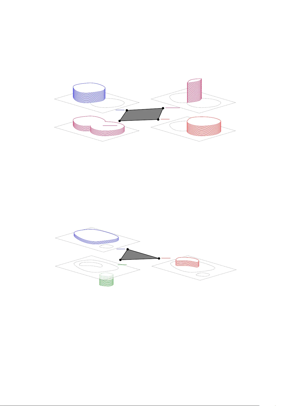
Exact reco v ery of the supp ort of piecewise constan t images via total v ariation regularization Y ohann De Castro 1 , Vincen t Duv al 2,3 , and Romain P etit ∗ 4 1 Institut Camille Jordan, CNRS UMR 5208, ´ Ecole Cen trale de Ly on, F-69134 ´ Ecully , F rance 2 CEREMADE, CNRS, UMR 7534, Univ ersit ´ e P aris-Dauphine, PSL Univ ersit y , 75016 P aris, F rance 3 INRIA-P aris, MOKAPLAN, 75012 P aris, F rance 4 MaLGa Cen ter, Departmen t of Mathematics, Univ ersit y of Genoa, 16146 Genoa, Italy April 1, 2024 Abstract This w ork is concerned with the reco v ery of piecewise constant images from noisy linear measuremen ts. W e study the noise robustness of a v ariational reconstruction method, whic h is based on total (gradien t) v ariation regularization. W e show that, if the unknown image is the sup erposition of a few simple shap es, and if a non-degenerate source condition holds, then, in the low noise regime, the reconstructed images hav e the same structure: they are the sup erposition of the same num b er of shapes, each a smo oth deformation of one of the unkno wn shap es. Moreov er, the reconstructed shapes and the asso ciated in tensities con v erge to the unknown ones as the noise go es to zero. 1 In tro duction 1.1 Reconstruction of images from noisy linear measuremen ts In their seminal work [ Rudin et al., 1992 ], Rudin, Osher and F atemi prop osed a celebrated de- noising method, whic h has the striking feature of removing noise from images while preserving their edges. This is ac hiev ed b y minimizing a functional with a regularization term, the to- tal (gradient) v ariation, whic h penalizes oscillations in the reconstructed image, while allowing for discon tin uities. This approac h was later applied outside the denoising setting, in order to solve general linear in verse problems (see e.g. [ Acar and V ogel, 1994 , Cha ven t and Kunisc h, 1997 ]). Although state of the art algorithms no w ha v e m uch better performance, this work pioneered the use of the total v ariation in imaging, and is still an imp ortan t baseline for image reconstruc- tion metho ds. It is well known that using the total v ariation as a regularizer promotes piecewise constant solutions. In denoising, for instance, Nik olov a has explained in [ Nikolo v a, 2000 ] that the non- diﬀeren tiabilit y of the regularizer tends create large ﬂat zones instead of oscillating regions (see also [ Ring, 2000 , Jalalzai, 2016 ]), whic h is known as the stair c asing eﬀe ct . Alternativ ely , in in v erse problems with few linear measuremen ts, it is possible to pro ve that some solutions to the v ariational problem are indeed piecewise constant, by appealing to a representation principle ∗ Most of this work was conducted when Romain Petit was aﬃliated with 2 , 3. 1 deriv ed in [ Boy er et al., 2019 , Bredies and Carioni, 2019 ] . Considering v ariational problems with a conv ex regularization term, they p ointed out the link b et w een the structural properties of the solutions on the one hand, and the structure of the unit ball deﬁned by the regularizer on the other hand. In the con text of total v ariation regularization, these results show that, under a few assumptions, some solutions are of the form P N i =1 a i 1 E i . This suggests that such functions are the sparse ob jects naturally asso ciated to this regularizer. In the presen t article, we follow this line of work and analyze total v ariation regularization from a new p ersp ectiv e, by drawing connections with the ﬁeld of sparse reco very . 1.2 Problem form ulation W e consider an unkno wn function u 0 ∈ L 2 ( R 2 ) whic h mo dels the image to reconstruct. W e assume that, in order to reco ver u 0 , w e hav e access to a set of linear observ ations y 0 = Φ u 0 , where Φ is deﬁned by: Φ : L 2 ( R 2 ) → H u 7→ ˆ R 2 ϕ ( x ) u ( x ) dx , with ϕ ∈ L 2 ( R 2 , H ) and H a separable Hilb ert space (typically R m or L 2 ( R 2 )). T o account for the presence of noise in the observ ations, we also consider the reco very of u 0 from y 0 + w where w ∈ H is an additive noise. F ollowing the abov e-mentioned w orks, we aim at reco v ering u 0 from y 0 b y solving inf u ∈ L 2 ( R 2 ) TV( u ) s.t. Φ u = y 0 , ( P 0 ( y 0 )) where TV ( u ), deﬁned b elow, denotes the total (gradient) v ariation of u . T o recov er u 0 from y 0 + w , w e solve instead, for some λ > 0, the following problem: inf u ∈ L 2 ( R 2 ) 1 2 ∥ Φ u − y ∥ 2 H + λ TV ( u ) , ( P λ ( y )) with y = y 0 + w . The question this work is concerned with is the follo wing: if w is small and λ well chosen, are the solutions of ( P λ ( y 0 + w ) ) close to some solutions of ( P 0 ( y 0 )) ? If u 0 is the unique so- lution to ( P 0 ( y 0 )) (in this case, we say that u 0 is identiﬁable ), answering p ositively amounts to proving that the considered v ariational metho d enjoys some noise robustness, i.e. that solv- ing ( P λ ( y 0 + w ) ) yields go o d approximations of u 0 in the low noise regime. T o our kno wledge, ﬁnding suﬃcient conditions for the iden tiﬁablity of u 0 is mostly open. Still, let us p oint out that, in [ Bredies and Vicente, 2019 ], an identiﬁabilit y result is obtained for the reco v ery of u 0 from its image under a linear partial diﬀerential op erator with unknown b oundary conditions. An exact recov ery result is also obtained in [ Holler and Wirth, 2022 ] in a diﬀeren t setting, where the regularizer is the so-called anisotr opic total v ariation. 1.3 Motiv ation In order to motiv ate our analysis, w e presen t in this subection a simple experiment show casing the phenomenon w e wish to analyze. W e consider an unknown image of the form u 0 = P N i =1 a i 1 E i , and deﬁne Φ as the conv olution with a Gaussian ﬁlter follo wed b y a subsampling on a regular grid of size 50 × 50. The noise is drawn from a m ultiv ariate Gaussian with a zero mean and an isotropic co v ariance matrix. Giv en these noisy observ ations y 0 + w , w e n umerically appro ximate a solution u λ,w of ( P λ ( y 0 + w ) ) using the metho d introduced in [ Condat, 2017 ], which is a discrete 2 (a) u 0 (b) y 0 + w (c) appro x. of u λ,w Figure 1: Numerical resolution of ( P λ ( y 0 + w ) ) for u 0 = 1 B (0 ,R ) . (a) u 0 (b) y 0 + w (c) appro x. of u λ,w Figure 2: Numerical resolution of ( P λ ( y 0 + w ) ) for u 0 = 1 E 1 + 2 1 E 2 − 2 1 E 3 . image deﬁned a grid 5 times ﬁner than the observ ation grid. W e notice that, for tw o diﬀerent c hoices of u 0 , the appro ximation of u λ,w has a structure whic h is close to that of u 0 . Up to discretization artifcats, it is the sup erp osition of the same num b er of shap es, each b eing close to one of the unknown shap es. In the present article, we wish to theoretically analyze this phenomenon. Our aim is to in v estigate whether, if u 0 is the sup erp osition of a few simple shap es, solutions of ( P λ ( y 0 + w ) ) ha v e the same structure. 1.4 Previous w orks T otal v ariation minimization in imaging. The theoretical study of total v ariation regu- larization in imaging was initiated in [ Cham b olle and Lions, 1997 , Ring, 2000 ]. Then, a lot of atten tion w as fo cused on the denoising case, which can be regarded as one step of the total v aria- tion gradient ﬂow, see [ Bellettini et al., 2002 , Alter et al., 2005b ]. Its connection to the Cheeger problem w as observ ed in [ Alter e t al., 2005a , Alter and Case lles, 2009 ] and w as the key to under- standing the prop erties of the Cheeger sets of conv ex b o dies. Let us also mention the landmark result [ Caselles et al., 2007 ], which shows that the jump set of the reconstructions is included in the jump set of the noisy input. Indep enden tly , Allard ga ve a precise description of the prop erties of the minimizers in the series of articles [ Allard, 2008a , Allard, 2008b , Allard, 2009 ]. W e refer to [ Cham b olle et al., 2010 ] for an in tro duction to total v ariation references and a m uch more comprehensiv e list of bibliographical references. Piecewise constan t images. Let us emphasize that the ab o ve-men tioned represen tation prin- ciple [ Bo yer et al., 2019 , Bredies and Carioni, 2019 ] only applies to inv erse problems with a ﬁ- 3 nite n umber of measurements. It do es not cov er the case of denoising or related tasks inv olving inﬁnite-dimensional observ ations. F or such cases, sev eral authors hav e prop osed sp eciﬁc ap- proac hes to promote piecewise constant solutions [ F ornasier, 2006 , F ornasier and March, 2007 , F onseca et al., 2010 , Cristoferi and F onseca, 2019 ]. These metho ds rely on the minimization of non-con v ex functionals which resem ble the ℓ 0 norm, while the total v ariation relates to the ℓ 1 norm. Noise robustness. The general conv ergence results presented in [ Burger and Osher, 2004 , Hofmann et al., 2007 ] apply to the case of total v ariation regularization, and lo osely sp eaking pro vide (under mild assumptions) strict con vergence in BV loc of solutions of ( P λ ( y 0 + w ) ) to- w ards solutions of ( P 0 ( y 0 )) . Moreo ver, in sp eciﬁc cases, the analysis in [ Burger and Osher, 2004 ] ensures that the v ariation of solutions to ( P λ ( y 0 + w ) ) is mostly concentrated in a neighborho o d of the supp ort of D u 0 . In [ Chambolle et al., 2017 , Iglesias et al., 2018 ], improv ed conv ergence guaran tees are derived b y exploiting the optimality of level sets of solutions of ( P λ ( y 0 + w ) ) for the prescribed curv ature problem. The main ﬁnding of these w orks is that, under a few assumptions, the b oundaries of the level sets conv erge in the Hausdorﬀ sense. Supp ort reco v ery in v ariational sparse regularization. In the litterature on v ariational sparse regularization, a line of work has sp eciﬁcally fo cused on strong noise robustness guarantees, called exact supp ort r e c overy or mo del identiﬁc ation . They were ﬁrst studied in the case of ﬁnite- dimensional ℓ 1 regularization. In this setting, it was prov ed in [ F uchs, 2004 ] and [ T ropp, 2006 ] that, under some conditions (called “irrepresentabilit y conditions” in the statistics comm unity , see [ Zhao and Y u, 2006 ]), solving the celebrated Lasso problem (the analog of ( P λ ( y ) )) allo ws to exactly recov er the support of the unkno wn sparse vector. Subsequen tly , it was shown in the landmark paper [ Candes et al., 2006 ] that these conditions are satisﬁed in the case of subsampled F ourier measurements. Later w orks established the exact recov ery of the group-supp ort for group-sparse vectors [ Bac h, 2008a ], of the rank for low-rank matrices [ Bach, 2008b ], or of more general structures enco ded in the singularities of partly-smo oth regularizers [ V aiter et al., 2018 ] or mirror-stratiﬁable functions [ F adili et al., 2018 ]. Oﬀ-the-grid sparse spik es recov ery and non-degeneracy assumptions. Bey ond ﬁnite- dimensional examples, sev eral works hav e inv estigated the case of total v ariation regulariza- tion on the space of Radon measures, where the unkno wn signal is a linear combination of Dirac masses (see [ De Castro and Gam b oa, 2012 ] and [ Bredies and Pikk arainen, 2013 ]). In that setting (contrary to that of the presen t pap er), suﬃcient iden tiﬁability conditions ha ve b een extensiv ely studied (see the landmark pap er [ Cand` es and F ernandez-Granda, 2014 ] and its gen- eralization [ Poon et al., 2023 ]). In [ Duv al and Peyr ´ e, 2015 ], a slight y stronger condition was in tro duced, called the non-de gener ate sour c e c ondition , whic h ensures the exact supp ort recov- ery prop erty in this inﬁnite-dimensional setting. More precisely , at low noise, the solutions to the Beurling Lasso problem (the analog of ( P λ ( y ) ) for measures) hav e the same num b er of atoms as the unkno wn measure, each close to one of the unknown atoms. Ensuring this condi- tion is a delicate issue. It was ﬁrst inv estigated numerically in [ Duv al and Peyr ´ e, 2015 ] for the decon v olution by the ideal low-pass ﬁlter with cutoﬀ frequency f c . Numerical evidence suggests that it is satisﬁed for measures whose atoms are separated by a distance of at least O (1 /f c ). The sp ecial case of p ositive atoms is somewhat simpler, and was inv estigated in dimension one in [ Deno yelle et al., 2017 , Duv al, 2019 ] and in higher dimension in [ Poon and Peyr ´ e, 2019 ]. Ev en tually , a general theoretical framew ork ensuring that condition pro vided the lo cations of the Dirac masses are suﬃcien tly separated was provided in [ Poon et al., 2023 ]. One striking feature of the non-de gener ate sour c e c ondition , compared to the standard ℓ 1 iden tiﬁabilit y condition, 4 is that it inv olves the second order deriv atives of some solution of the dual problem. It is not kno wn whether the stability of the supp ort holds under weak er assumptions, but there are coun- terexamples of measures which are identiﬁable (i.e., they are the unique solution to the noiseless problem) but their supp ort is not stable at any noise level, see [ Duv al, 2022 , Chapter 5]. Thus, some additional assumption is needed, and the condition on the second deriv atives ﬁlls that gap. It is therefore natural that, in the present pap er, our analysis of the total (gradien t) v ariation supp ort recov ery prop ert y relies on the non-degeneracy of some second deriv atives. Let us men- tion, inciden tally , that the recen t work [ Carioni and Grande, 2023 ], which studies the stability of sparse representations in conv ex optimization in volv es a similar criterion 1 . 1.5 Con tributions The ab o ve-men tioned w orks on total (gradien t) v ariation regularization provide little information ab out the structure of solutions to ( P λ ( y 0 + w ) ) in the lo w noise regime. Ho wev er, in light of the n umerical evidence presen ted in Section 1.3 , the following question is natural: if u 0 is iden tiﬁable and is the sum of a few indicator functions, do the solutions of ( P λ ( y 0 + w ) ) hav e a similar prop ert y? Moreo ver, are these decomp ositions stable, i.e. are they made of the same num b er of atoms, and are their atoms related? In this work, we answer these questions by using tw o main to ols. The ﬁrst is a set of results ab out the faces of the unit ball deﬁned by the total v ariation, which provide useful information on the ab ov e-mentioned decomp ositions. The second is an analysis of the b ehaviour of solutions to the prescrib ed curv ature problem under v ariations of the curv ature functional. T o state our main result, we introduce a non-degenerate version of the source condition, whic h relies on a regularity assumption on the measurement op erator Φ, namely that ϕ ∈ C 1 ( R 2 , H ). This cov ers a wide v ariet y of forward op erators that are of particular in terest for applications. T o name only a few, let us cite the case of the conv olution with a Gaussian blur (or more generally , with any C 1 ﬁlter) p ossibly follow ed by a subsampling, or a motion blur, of particular in terest in computational photography . Let us also mention the case of subsampled F ourier measuremen ts, of particular in terest in X-ray tomography , magnetic resonance imaging and radio interferometry . Ho w ever, it do es not cov er the case of denoising, 2 whic h corresp onds to H = L 2 ( R 2 ) and Φ = Id. In all the follo wing, except in Section 2 in which we review existing results, we assume that ϕ ∈ C 1 ( R 2 , H ). Our main result, whic h is Theorem 5.4 , informally states that, if the unkno wn image mo deled b y u 0 is the sup erp osition of a few simple shap es and the non-degenerate source condition holds, then, in the low noise regime, every solution u λ,w of ( P λ ( y 0 + w ) ) is made of the same num b er of shap es as u 0 , eac h shap e in u λ,w con v erging smo othly to the corresp onding shap e in u 0 as the noise go es to zero (see Figure 3 for an illustration). 2 Preliminaries 2.1 Smo oth sets and normal deformations Our analysis mainly concerns the level sets of the solutions to ( P 0 ( y 0 ) ) and ( P λ ( y ) ). As w e strongly rely on their regularity , we recall here several deﬁnitions and prop erties related to 1 How ever, as underlined by the authors of [ Carioni and Grande, 2023 ], their analysis do es not co ver our setting. 2 Although it is counterin tuitive, we conjecture that the denoising case is less fa vorable to support recov ery . F or instance, it is known that when u 0 is the indicator of a square (with rounded corners), the solution of ( P λ ( y ) ) has inﬁnitely many level lines for any λ > 0 small enough, see [ Chambolle et al., 2010 ]. 5 A B (a) u 0 A λ,w B λ,w (b) u λ,w Figure 3: Illustration of the result stated in Theorem 5.4 . Here u 0 is equal to 0 in A and B . The v alues taken by u λ,w in A λ,w and B λ,w are close (but not necessarily equal) to 0. smo oth sets and their normal deformations. W e refer to [ Delfour and Zolesio, 2011 ] for more details. Smo oth set. Let E ⊂ R 2 b e an op en set such that ∂ E  = ∅ and k ∈ N ∗ , where N ∗ def. = { 1 , 2 , ... } denotes the set of p ositive integers. W e say that the set E is of class C k if, for ev ery x ∈ ∂ E , there exists r x > 0, a rotation matrix R x , and a function u x ∈ C k ([ − r x , r x ]) such that ( R − 1 x ( E − x ) ∩ C (0 , r x ) = { ( z , t ) ∈ C (0 , r x ) | t < u x ( z ) } def. = h yp ograph( u x ) , R − 1 x ( ∂ E − x ) ∩ C (0 , r x ) = { ( z , t ) ∈ C (0 , r x ) | t = u x ( z ) } def. = graph( u x ) , where C (0 , r ) def. = ( − r, r ) 2 . In that case, one can c ho ose u x (0) = 0 and ∇ u x (0) = 0. Moreov er, if ∂ E is compact, r x can b e taken independent of x , and the family { u x } x ∈ ∂ E uniformly equicon- tin uous (see [ Delfour and Zolesio, 2011 , Theorem 5.2]). In lo cal co ordinates, the outw ard unit normal to E at ( z , u x ( z )) is given by ν E ( z , u x ( z )) = 1 p 1 + u ′ x ( z ) 2  − u ′ x ( z ) 1  . It is a geometric quantit y , which does not depend on the choice of r , x and u x . Lik ewise, the signed curv ature of E at ( z , u x ( z )) is given by H E ( z , u x ( z )) = − u ′ x p 1 + u ′ 2 x ! ′ ( z ) = − u ′′ x ( z ) (1 + u ′ ( z ) 2 ) 3 / 2 . 6 Remark 2.1 The same deﬁnitions and pr op erties hold when r eplacing C k with C k,ℓ the sp ac e of k -times c ontinuously diﬀer entiable functions whose k -th derivative is ℓ -H¨ older ( 0 < ℓ ≤ 1 ). Leb esgue equiv alence classes and smo oth sets. If E ⊂ R 2 is an open set of class C 1 and x ∈ R 2 , then its Leb esgue density exists ev erywhere and it is given b y θ E ( x ) def. = lim r → 0 + | E ∩ B ( x, r ) | | B ( x, r ) | =      1 if x ∈ E , 1 / 2 if x ∈ ∂ E , 0 if x ∈ R 2 \ E . (1) When working with measurable sets, it is common to regard them mo dulo L eb esgue ne gligible sets . The ab o v e equality sho ws that if a measurable set ˜ E ∈ R 2 is equiv alent to a C 1 op en set E , then E is unique and can be reco vered as the set of Lebesgue points of ˜ E , that is { θ ˜ E = 1 } . In the following, we usually w ork with Leb esgue equiv alence classes. When E has a C 1 op en represen tativ e, we say that E is of class C 1 , and we denote by ∂ E the top ological b oundary of that representativ e. Con vergence. Let us deﬁne the square of axis ν ∈ S 1 and side r > 0 centered at x ∈ R 2 : C ( x, r, ν ) def. = x + R ν C (0 , r ) . (2) where R ν : R 2 → R 2 is the rotation that maps (0 , 1) to ν . Let E b e a set of class C k suc h that ∂ E is compact. W e say that a sequence ( E n ) n ∈ N con v erges to E in C k if there exists r > 0 and n 0 ∈ N such that • for every n ≥ n 0 w e hav e ∂ E n ⊂ S x ∈ ∂ E C ( x, r, ν E ( x )) • for every n ≥ n 0 and x ∈ ∂ E there exists u n,x ∈ C k ([ − r , r ]) such that: ( R − 1 ν E ( x ) ( ∂ E n − x ) ∩ C (0 , r ) = graph( u n,x ) R − 1 ν E ( x ) (in t E n − x ) ∩ C (0 , r ) = hypograph( u n,x ) • denoting ( u x ) x ∈ ∂ E some functions satisfying ( R − 1 ν E ( x ) ( ∂ E − x ) ∩ C (0 , r ) = graph( u x ) R − 1 ν E ( x ) (in t E − x ) ∩ C (0 , r ) = hypograph( u x ) w e hav e lim n → + ∞ sup x ∈ ∂ E ∥ u n,x − u x ∥ C k ([ − r,r ]) = 0 Normal deformation. W e state b elow some useful results regarding normal deformations of a smooth set E . First, let us stress that such sets are parametrized b y real-v alued functions on ∂ E , which leads us to use the notion of tangen tial gradient, tangen tial Jacobian, and the spaces C k ( ∂ E ), L p ( ∂ E ) and H 1 ( ∂ E ) (along with their asso ciated norms). W e refer to the reader to [ Henrot and Pierre, 2018 , Section 5.4.1, 5.4.3 and 5.9.1] for precise deﬁnitions. Lemma 2.2 If E is a b ounde d set of class C k ( k ≥ 2 ), then ther e exists C > 0 such that, for every φ in C k − 1 ( ∂ E ) , the mapping φ ν E c an b e extende d to ξ φ ∈ C k − 1 ( R 2 , R 2 ) with ∥ ξ φ ∥ C k − 1 ( R 2 , R 2 ) ≤ C ∥ φ ∥ C k − 1 ( ∂ E ) . 7 Prop osition 2.3 L et E b e a b ounde d op en set of class C k (with k ≥ 2 ). Ther e exists c > 0 such that, for every φ ∈ C k − 1 ( ∂ E ) with ∥ φ ∥ C k − 1 ( ∂ E ) ≤ c , ther e is a unique b ounde d op en set of class C k − 1 , denote d E φ , satisfying ∂ E φ = ( I d + φ ν E )( ∂ E ) . (3) Mor e over, ther e exists an extension ξ φ of φ ν E such that E φ = ( I d + ξ φ )( E ) and ∥ ξ φ ∥ C k − 1 ( R 2 , R 2 ) < 1 . In p articular, E φ is C k − 1 -diﬀe omorphic to E . Prop osition 2.4 If ( E n ) n ≥ 0 c onver ges to a b ounde d set E in C k with k ≥ 2 , then for n lar ge enough ther e exists φ n ∈ C k − 1 ( ∂ E ) such that E n = E φ n , and ∥ φ n ∥ C k − 1 ( ∂ E ) → 0 . 2.2 F unctions of b ounded v ariation and sets of ﬁnite p erimeter W e recall here a few prop erties of functions of bounded v ariation and sets of ﬁnite perimeter. More details can b e found in the monogaphs [ Ambrosio et al., 2000 , Maggi, 2012 ]. The total v ariation. The total v ariation of a function u ∈ L 1 loc ( R 2 ) is given by TV( u ) def. = sup  − ˆ R 2 u div z     z ∈ C ∞ c ( R 2 , R 2 ) , ∥ z ∥ ∞ ≤ 1  . If TV( u ) is ﬁnite, then u is said to ha ve b ounded v ariation, and its distributional gradient D u is a ﬁnite Radon measure. In that case, w e ha v e | D u | ( R 2 ) = TV ( u ). In all the following, we consider TV as a mapping from L 2 ( R 2 ) to R ∪ { + ∞} . This mapping is conv ex, prop er and low er semi-con tin uous. Sets of ﬁnite p erimeter. If a measurable set E ⊂ R 2 is such that P ( E ) def. = TV( 1 E ) < + ∞ , it is said to b e of ﬁnite p erimeter. If E is an op en set of class C 1 , then P ( E ) is simply the length of its top ological b oundary , P ( E ) = H 1 ( ∂ E ), where H 1 denotes the one-dimensional Hausdorﬀ measure. Coarea form ula F unctions with b ounded v ariation and sets of ﬁnite perimeter are related through the coarea formula [ Ambrosio et al., 2000 , Thm. 3.40]. F or u ∈ L 1 loc ( R 2 ) and t ∈ R , we consider the level sets of u , U ( t ) def. = ( { x ∈ R 2 | u ( x ) ≥ t } if t ≥ 0 , { x ∈ R 2 | u ( x ) ≤ t } otherwise. (4) It is worth noting that, if u ∈ L 2 ( R 2 ), then | U ( t ) | < + ∞ for all t  = 0. The coarea formula states that ∀ u ∈ L 2 ( R 2 ) , TV( u ) = ˆ + ∞ −∞ P ( U ( t ) )d t. (5) 8 The isop erimetric inequality . F or every set of ﬁnite p erimeter E , the isop erimetric inequal- it y states that p min( | E | , | E c | ) ≤ c 2 P ( E ) , (6) with equality if and only if E is a ball, and where c 2 def. = 1 / √ 4 π is the isop erimetric constant (see e.g. [ Maggi, 2012 , Chapter 14]). In particular, if E is a set of ﬁnite p erimeter, either E or E c has ﬁnite measure. As a consequence of ( 6 ) and the coarea formula, the following Poincar ´ e-t yp e inequalit y holds (see [ Ambrosio et al., 2000 , Theorem 3.47]), ∀ u ∈ L 2 ( R 2 ) , ∥ u ∥ 2 ≤ c 2 TV( u ) . (7) Indecomp osable and simple sets. A set of ﬁnite p erimeter E ⊂ R 2 is said to be decom- p osable if there exists a partition of E in tw o sets of p ositive Leb esgue measure A and B with P ( E ) = P ( A ) + P ( B ). W e sa y that E is indecomposable if it is not decomp osable. W e sa y that a measurable set E is simple if E = R 2 , or | E | < + ∞ and b oth E and R 2 \ E are indecomp osable. The imp ortance of simple sets stems from their connection with the extreme p oin ts of the total v ariation unit ball. Prop osition 2.5 ([ Fleming, 1957 , Ambrosio et al., 2001 ]) The extr eme p oints of the c onvex set { TV ≤ 1 } def. =  u ∈ L 2 ( R 2 )   TV( u ) ≤ 1  ar e the functions of the form ± 1 E /P ( E ) , wher e E is a simple set with 0 < | E | < + ∞ . Ho w ever, it is worth noting that the exp ose d p oints of { TV ≤ 1 } in the L 2 top ology (i.e. p oin ts that are the only maximizer ov er { TV ≤ 1 } of a contin uous linear form on L 2 ( R 2 )) hav e m uc h more structure (see Sections 3 and 3.3 ). 2.3 Sub diﬀeren tial of the total v ariation Let us now collect several results on the subdiﬀerential of TV , which are useful to deriv e and analyze the dual problems of ( P 0 ( y 0 )) and ( P λ ( y )) . Since TV : L 2 ( R 2 ) → R ∪ { + ∞} is the supp ort function of the conv ex set C def. =  div z   z ∈ C ∞ c ( R 2 , R 2 ) , ∥ z ∥ ∞ ≤ 1  , its sub diﬀeren tial at 0 is the closure of C in L 2 ( R 2 ), that is ∂ TV(0) = C =  div z   z ∈ L ∞ ( R 2 , R 2 ) , div z ∈ L 2 ( R 2 ) , || z || ∞ ≤ 1  . (8) W e also hav e the following useful iden tity: ∂ TV(0) =  η ∈ L 2 ( R 2 )     ∀ u ∈ L 2 ( R 2 ) ,     ˆ R 2 η u     ≤ TV ( u )  . (9) Finally , the sudiﬀerential of TV at some u ∈ L 2 ( R 2 ) is given by: ∂ TV( u ) =  η ∈ ∂ TV(0)     ˆ R 2 η u = TV ( u )  . (10) Hence, if η ∈ ∂ TV( u ), then η is an elemen t of ∂ TV (0) = C for whic h the suprem um in the deﬁnition of the total v ariation is attained. 9 2.4 Dual problems and dual certiﬁcates The backbone of our main result is the relation b etw een the solutions of ( P 0 ( y 0 )) or ( P λ ( y )) and the solutions of their dual problems. W e gather here several properties of these dual problems whic h can b e found in [ Chambolle et al., 2017 ] (for the denoising case) and [ Iglesias et al., 2018 , Section 2] (for the general case). Dual problems. The F enchel-Rock afellar dual problems to ( P 0 ( y 0 )) and ( P λ ( y )) are resp ec- tiv ely sup p ∈H ⟨ p, y 0 ⟩ H s.t. Φ ∗ p ∈ ∂ TV (0) , ( D 0 ( y 0 )) sup p ∈H ⟨ p, y ⟩ H − λ 2 || p || 2 H s.t. Φ ∗ p ∈ ∂ TV (0) . ( D λ ( y )) The existence of a solution to ( D 0 ( y 0 )) does not alw ays hold. On the contrary , ( D λ ( y )) can be reform ulated as the problem of pro jecting y /λ onto the closed conv ex set { p ∈ H | Φ ∗ p ∈ ∂ TV (0) } , whic h has a unique solution. Strong dualit y . F rom [ Iglesias et al., 2018 , Theorem 1], the v alues of ( P 0 ( y 0 )) and ( D 0 ( y 0 )) are equal. Moreo ver, if there exists a solution p to ( D 0 ( y 0 )) , then for every solution u of ( P 0 ( y 0 )) w e hav e Φ ∗ p ∈ ∂ TV ( u ) . (11) Con v ersely , if ( u, p ) ∈ L 2 ( R 2 ) × H with Φ u = y 0 and (11) holds, then u and p resp ectively solv e ( P 0 ( y 0 )) and ( D 0 ( y 0 )) . F rom the p ersp ective of in verse problems, given some unkno wn image u 0 ∈ L 2 ( R 2 ) and observ ation y 0 = Φ u 0 , it is therefore suﬃcient to assume the existence of p ∈ H with Φ ∗ p ∈ ∂ TV ( u 0 ) to ensure that u 0 is a solution to ( P 0 ( y 0 )) . This prop erty is kno wn as the sour c e c ondition [ Neubauer, 1989 , Burger and Osher, 2004 ]. If, moreov er, Φ is injective on the cone { u ∈ L 2 ( R 2 ) | Φ ∗ p ∈ ∂ TV ( u ) } , then u 0 is the unique solution to ( P 0 ( y 0 )) . As in the noiseless case, the v alues of ( P λ ( y )) and ( D λ ( y )) are equal. Moreov er, denoting b y p the unique solution to ( D λ ( y )) , for ev ery solution u of ( P λ ( y )) we ha v e ( Φ u = y − λ p , Φ ∗ p ∈ ∂ TV ( u ) . (12) Con v ersely , if (12) holds, then u and p resp ectively solv e ( P λ ( y )) and ( D λ ( y )) . Although there migh t not b e a unique solution to ( P λ ( y )) , (12) yields that all of them ha v e the same image b y Φ and the same total v ariation. Dual certiﬁcates. If η = Φ ∗ p and η ∈ ∂ TV( u ), we call η a dual certiﬁcate for u with resp ect to ( P 0 ( y 0 )) , as its existence certiﬁes the optimality of u for ( P 0 ( y 0 )) , pro vided y 0 = Φ u . Similarly , if η = − Φ ∗ (Φ u − y ) /λ and η ∈ ∂ TV ( u ), we call η a dual certiﬁcate for u with resp ect to ( P λ ( y )) . There could b e multiple dual certiﬁcates asso ciated to ( P 0 ( y 0 )) . One of them, the minimal norm certiﬁcate, plays a crucial role in the analysis of the low noise regime. A quic k lo ok at the ob jectiv e of ( D λ ( y )) indeed suggests that, as λ go es to 0, its solution conv erges to the solution to the limit problem ( D 0 ( y 0 )) with minimal norm. This is Proposition 2.7 b elow. Deﬁnition 2.6 If ther e exists a solution to ( D 0 ( y 0 )) , the minimal norm dual c ertiﬁc ate asso ci- ate d to ( P 0 ( y 0 )) , denote d η 0 , is deﬁne d as η 0 = Φ ∗ p 0 with p 0 = argmin ∥ p ∥ H s.t. p solves ( D 0 ( y 0 )) . 10 If λ > 0, w e denote p λ,w the unique solution to ( D λ ( y 0 + w ) ), and η λ,w = Φ ∗ p λ,w the asso ciated dual certiﬁcate. Noise robustness results extensively rely on the b ehaviour of η λ,w as λ and w go to zero. This b ehaviour is describ ed b y the following results. Prop osition 2.7 ([ Chambolle et al., 2017 , Prop.6],[ Iglesias et al., 2018 , Prop. 3]) If ther e exists a solution to ( D 0 ( y 0 )) , then p λ, 0 c onver ges str ongly to p 0 as λ → 0 . Since p λ,w is the pro jection of ( y 0 + w ) /λ onto the closed conv ex set { p ∈ H | Φ ∗ p ∈ ∂ TV (0) } , the non-expansiveness of the pro jection mapping yields ∀ ( λ, w ) ∈ R ∗ + × H , ∥ p λ,w − p λ, 0 ∥ H ≤ ∥ w ∥ H λ , (13) and hence ∀ ( λ, w ) ∈ R ∗ + × H , ∥ η λ,w − η λ, 0 ∥ L 2 ( R 2 ) ≤ ∥ Φ ∗ ∥ ∥ w ∥ H λ . As a result, if λ → 0 and ∥ w ∥ H /λ → 0, the dual certiﬁcate η λ,w con v erges strongly in L 2 ( R 2 ) to the minimal norm certiﬁcate η 0 . 2.5 Noise robustness results Let us now review existing noise robustness results, whic h we use in v arious parts of this w ork. F rom Prop osition 3.1 and the results of Section 2.4 , we know that the levels sets of solutions to ( P λ ( y 0 + w ) ) are solution to the prescribed curv ature problem asso ciated to η λ,w . In [ Chambolle et al., 2017 , Iglesias et al., 2018 ], this fact is exploited to obtain uniform prop er- ties of the lev el sets in the lo w noise regime. W e collect the byproducts of this analysis in the follo wing lemma. Lemma 2.8 ([ Cham b olle et al., 2017 , Section 5]) L et ( η n ) n ≥ 0 ⊂ ∂ TV (0) b e a se quenc e c onver g- ing str ongly in L 2 ( R 2 ) to η ∞ , and let E b e deﬁne d by E def. =  E ⊂ R 2 , 0 < | E | < + ∞     ∃ n ∈ N ∪ {∞} , P ( E ) =     ˆ E η n      . Then the fol lowing holds: 1. inf E ∈E P ( E ) > 0 and sup E ∈E P ( E ) < + ∞ , 2. inf E ∈E | E | > 0 and sup E ∈E | E | < + ∞ , 3. ther e exists R > 0 such that, for every E ∈ E , it holds E ⊂ B (0 , R ) , 4. ther e exists r 0 > 0 and C ∈ (0 , 1 / 2) such that for every r ∈ (0 , r 0 ] and E ∈ E : ∀ x ∈ ∂ E , C ≤ | E ∩ B ( x, r ) | | B ( x, r ) | ≤ 1 − C . 11 In the ab ov e-mentioned works, Lemma 2.8 is used to obtain the conv ergence result of Prop o- sition 2.9 . It indeed allows to sho w that, in the low noise regime, the solutions to ( P λ ( y 0 + w ) ) ha v e b ounded supp ort, and therefore b elong to L 1 ( R 2 ). This can in turn b e used to sho w their strict conv ergence in BV( R 2 ) tow ards a solution u ∗ of ( P 0 ( y 0 )) , whic h in particular imply the w eak-* con vergence of their gradient (see e.g. [ Ambrosio et al., 2000 , Prop osition 3.13 and Def- inition 3.14]). Finally , one obtains the conv ergence of their level set tow ards those of u ∗ in the Hausdorﬀ sense, whic h corresp onds to the uniform conv ergence of the associated distance functions (see Theorem 6.1 and its proof in [ Ambrosio et al., 2000 ]). Prop osition 2.9 Assume ( D 0 ( y 0 )) has a solution, λ n → 0 and ∥ w n ∥ H λ n ≤ 1 4 c 2 ∥ Φ ∗ ∥ . Then, if u n is a solution of ( P λ n ( y 0 + w n ) ) for al l n ∈ N , we have that (Supp( u n )) n ≥ 0 is b ounde d and that, up to the extr action of a subse quenc e (not r elab ele d), ( u n ) n ≥ 0 c onver ges strictly in BV ( R 2 ) to a solution u ∗ of ( P 0 ( y 0 )) . Mor e over, for almost every t ∈ R , we have:   U ( t ) n △ U ( t ) ∗   − → 0 and ∂ U ( t ) n − → ∂ U ( t ) ∗ , wher e the last limit holds in the Hausdorﬀ sense 3 . 3 The exp osed faces of the total v ariation unit ball W e recall that, in the remaining of this w ork, we assume that ϕ ∈ C 1 ( R 2 , H ), so that Φ ∗ is con tin uous from H to C 1 ( R 2 ). In order to tak e adv antage of the extremality relations ( 11 ) and ( 12 ), it is imp ortant to understand the prop erties of u implied by the relation η ∈ ∂ TV ( u ), for a given η ∈ ∂ TV (0). In other words, our goal is to study the set ∂ TV ∗ ( η ) =  u ∈ L 2 ( R 2 )   η ∈ ∂ TV( u )  = Argmax u ∈ L 2 ( R 2 )  ˆ R 2 η u − TV ( u )  , (14) where TV ∗ denotes the F enchel conjugate of TV. 3.1 Subgradien ts and exp osed faces It is p ossible to relate ( 14 ) to the faces of the total v ariation unit ball, in connection with Fleming’s result (i.e. Prop osition 2.5 ). W e sa y that a set F ⊆ { TV ≤ 1 } is an exp osed face of { TV ≤ 1 } if there exists η ∈ L 2 ( R 2 ) such that F = Argmax u ∈{ TV ≤ 1 } ˆ R 2 η u . (15) Exp osed faces are closed conv ex subsets of { TV ≤ 1 } , and they are faces in the classical sense: if u ∈ F and I ⊂ { TV ≤ 1 } is an op en line segment containing u , then I ⊂ F . W e refer the reader to [ Ro ck afellar, 1970 , Chapter 18] for more detail on faces and exp osed faces. T o emphasize the dep endency on η we sometimes write F η for F , and w e note that F 0 = { TV ≤ 1 } and F tη = F η for all t > 0 . 3 See e.g. [ Ro ck afellar and W ets, 1998 , Chapter 4] for a deﬁnition. 12 It is also worth considering the corresp onding v alue, which is sometimes called the G -norm 4 in the literature [ Meyer, 2001 , Aujol et al., 2005 , Kindermann et al., 2006 , Haddad, 2007 ], ∀ η ∈ L 2 ( R 2 ) , ∥ η ∥ G def. = sup u ∈{ TV ≤ 1 } ˆ R 2 η u . In view of ( 9 ), we see that η ∈ ∂ TV (0) if and only if ∥ η ∥ G ≤ 1. Assuming that ∥ η ∥ G ≤ 1, the condition ´ R 2 η u = TV( u ) in ( 10 ) is equiv alent to u = 0 or ˆ R 2 η  u TV( u )  = 1 , (16) the latter equalit y implying that ∥ η ∥ G = 1 and u/ TV ( u ) ∈ F η . As a result, we obtain the follo wing description, TV ∗ ( η ) =      ∅ if ∥ η ∥ G > 1 , { 0 } ∪  S t> 0 ( t F η )  , if ∥ η ∥ G = 1, { 0 } if ∥ η ∥ G < 1 . (17) T o summarize the connection betw een subgradients and exp osed faces, if F is a face of { TV ≤ 1 } exp osed b y some η ∈ L 2 ( R 2 ) \ { 0 } , its conic h ull R + F is equal to ∂ TV ∗ ( η / ∥ η ∥ G ). Conv ersely , if ∥ η ∥ G = 1, then ∂ TV ∗ ( η ) ∩ { TV = 1 } is F η , the face of { TV ≤ 1 } exp osed by η . In the rest of this section, we ﬁx some η ∈ L 2 ( R 2 ) such that ∥ η ∥ G = 1 (the only in teresting case), and we study TV ∗ ( η ). Equiv alently , w e describ e all the faces of { TV ≤ 1 } exp osed by nonzero vectors. 3.2 Exp osed v ersus non-exp osed faces The extreme p oints of { TV ≤ 1 } are describ ed b y Prop osition 2.5 : those are the (signed, renormalized) indicators of simple sets. The k -dimensional faces ( k ∈ N ) are more complex, and they in volv e functions whic h are piecewise constan t on some partition of R 2 (see for in- stance [ Duv al, 2022 ], or the monographs [ F ujishige, 2005 , Bach, 2013 ] in a ﬁnite-dimensional setting). Ev en though it is known that the k -dimensional faces hav e a ﬁnite num b er of extreme p oin ts and are thus p olytop es (see [ Duv al, 2022 , Theorem 2.1]), the corresp onding partition can b e singular and counter-in tuitive [ Boy er et al., 2023 ]. Ho w ever, the faces inv olved in ( 17 ) are the exp ose d faces, and we emphasize in this section that they hav e a simpler structure than arbitray faces, esp ecially if η ∈ C 1 , as is the case in the extremalit y conditions ( 11 ) and ( 12 ). W e prov e in Theorem 3.8 that, under this assumption, the k -dimensional exposed faces of { TV ≤ 1 } are k -simplices. A t the core of our discussion is the reformulation of the sub diﬀerential prop erty into a geo- metric v ariational problem using level sets and the coarea formula (see ( 4 ) and ( 5 )). Prop osition 3.1 ([ Kindermann et al., 2006 , Chambolle et al., 2017 ]) L et u ∈ L 2 ( R 2 ) b e such that TV ( u ) < + ∞ , and let η ∈ L 2 ( R 2 ) . Then the fol lowing c onditions ar e e quivalent. (i) η ∈ ∂ TV ( u ) . 4 The G -norm is the p olar of the total v ariation (see [ Ro ck afellar, 1970 , Ch. 15]). It is p ossible to prov e that the G -norm is indeed a norm on L 2 ( R 2 ), in particular 0 < ∥ η ∥ G < + ∞ for all η ∈ L 2 ( R 2 ) \ { 0 } , see [ Haddad, 2007 ]. 13 (ii) η ∈ ∂ TV (0) and the level sets of u satisfy ∀ t > 0 , P ( U ( t ) ) = ˆ U ( t ) η and ∀ t < 0 , P ( U ( t ) ) = − ˆ U ( t ) η . (iii) The level sets of u satisfy ∀ t > 0 , U ( t ) ∈ Argmin E ⊂ R 2 , | E | < + ∞  P ( E ) − ˆ E η  , ∀ t < 0 , U ( t ) ∈ Argmin E ⊂ R 2 , | E | < + ∞  P ( E ) + ˆ E η  . 3.3 The prescrib ed curv ature problem The geome tric v ariational problem app earing in Prop osition 3.1 , inf E ⊂ R 2 , | E | < + ∞ J ( E ) def. = P ( E ) − ˆ E η , ( P C ( η )) is called the pr escrib e d curvatur e pr oblem asso ciated to η . This terminology stems from the fact that, if η is suﬃciently regular, every solution to ( P C ( η )) has a (scalar) distributional curv ature (see [ Maggi, 2012 , Section 17.3] for a deﬁnition) equal to η . This problem plays a crucial role in the analysis of total v ariation regularization, as explained b elo w. F or no w, let us gather some prop erties of that problem. Existence of minimizers. Solutions to ( P C ( η )) exist provided η ∈ ∂ TV(0). Indeed, the ob jectiv e J is nonnegativ e, and equal to zero for E = ∅ . F rom Prop osition 3.1 , we also kno w there is a non-empty solution as so on as η ∈ ∂ TV ( u ) for some u ∈ L 2 ( R 2 ) \ { 0 } . Boundedness. By [ Cham b olle et al., 2017 , Lemma 4], all solutions of ( P C ( η )) are included in some common ball, i.e. there exists R > 0 such that, for every solution E of ( P C ( η )) , w e ha v e E ⊂ B (0 , R ). Regularit y of the solutions. The regularit y of the solutions to ( P C ( η )) is well understo o d. If η is only assumed to b e square integrable, the solutions can b e singular but they ha ve some w eak form of regularit y , as shown in [ Gonzales et al., 1993 ]. In particular, it is known that the square C = [0 , 1] 2 is not a solution to ( P C ( η )) for an y η ∈ L 2 ( R 2 ) (see, e.g. [ Meyer, 2001 ]). As a result, the function 1 C /P ( C ) is an extr eme p oint of { TV ≤ 1 } which is not exp ose d. More regularit y can b e obtained by strengthening the integrabilit y and smo othness of η . If, in addition to being square integrable, η ∈ L ∞ loc ( R 2 ) (which ensures that η ∈ L ∞ ( B (0 , R ))), then any solution to ( P C ( η ) ) is a strong quasi-minimizer of the p erimeter, and, consequen tly , is equiv alent to an open set of class C 1 , 1 (see e.g. [ Ambrosio, 2010 , Deﬁnition 4.7.3 and Theorem 4.7.4]). F urthermore, if η is con tin uous, then the b oundary of an y solution is lo cally the graph of a function u whic h solves (in the sense of distributions) the Euler-Lagrange equation asso ciated to ( P C ( η ) ), that is (up to a translation and a rotation): u ′ p 1 + u ′ 2 ! ′ ( z ) = η ( z , u ( z )) . (18) This in turn implies that u is C 2 (C k +2 ,α if η ∈ C k,α ( R 2 )) and solves (18) in the classical sense. 14 3.4 Indicator functions corresp onding to a giv en face W e ﬁx η ∈ L 2 ( R 2 ) suc h that ∥ η ∥ G = 1 (hence η ∈ ∂ TV (0)), and w e study the face F of { TV ≤ 1 } exp osed b y η . W e assume in addition that η ∈ C 1 ( R 2 ). As we kno w that the extreme p oints of F m ust b e (signed, renormalized) indicators of simple sets, it is natural to fo cus on suc h functions. The main result w e pro ve in this section is the follo wing. Prop osition 3.2 F or any extr eme p oint u of F , ther e exists a unique p air ( s, E ) , wher e E is a simply c onne cte d op en set of class C 3 and s ∈ {− 1 , 1 } , such that u = s 1 E /P ( E ) . If u 1 and u 2 ar e two distinct extr eme p oints of F , and { ( s i , E i ) } i =1 , 2 ar e their c orr esp onding de c omp ositions, then ∂ E 1 ∩ ∂ E 2 = ∅ . T o obtain this result, we study the elements of F whic h are (prop ortional to) indicator functions, and we introduce the collection E def. = E + ∪ E − ∪ {∅ , R 2 } , where E + def. =  E ⊂ R 2     | E | < + ∞ , 0 < P ( E ) < + ∞ , 1 E P ( E ) ∈ F  , E − def. =  E ⊂ R 2     | E c | < + ∞ , 0 < P ( E c ) < + ∞ , − 1 E c P ( E c ) ∈ F  . (19) If | E | < + ∞ (resp. | E | = + ∞ ), Prop osition 3.1 ab ov e shows that E ∈ E + (resp. E ∈ E − ) if and only if E is a solution to ( P C ( η ) ) (resp. E c is a solution to P C ( − η )). 3.4.1 Structure of E The collection E has the remark able prop erty of being closed under union and intersection. Prop osition 3.3 L et E ∈ E and F ∈ E . Then E ∩ F ∈ E and E ∪ F ∈ E . In fact, E is ev en closed under c ountable union and intersection, but we do not need this prop ert y here. Pr o of. If E ∈ E + and F ∈ E + the submo dularity of the p erimeter (see e.g. [ Ambrosio et al., 2001 , Prop osition 1]) yields: P ( E ∩ F ) + P ( E ∪ F ) ≤ P ( E ) + P ( F ) = ˆ E η + ˆ F η = ˆ E ∩ F η + ˆ E ∪ F η . W e hence obtain:  P ( E ∩ F ) − ˆ E ∩ F η  +  P ( E ∪ F ) − ˆ E ∪ F η  ≤ 0 . By ( 9 ), the ab ov e tw o terms are nonnegative, whic h yields E ∩ F ∈ E + (unless E ∩ F = ∅ ) and E ∪ F ∈ E + . The same argumen t applies to the complemen ts, when b oth E and F are 15 in E − . No w, if E ∈ E + and F ∈ E − , P ( E ∩ F ) + P (( E ∪ F ) c ) = P ( E ∩ F ) + P ( E ∪ F ) ≤ P ( E ) + P ( F ) = P ( E ) + P ( F c ) = ˆ E η − ˆ F c η = ˆ E ∩ F η − ˆ ( E ∪ F ) c η Reasoning as ab ov e, we obtain that E ∩ F ∈ E + (unless E ∩ F = ∅ ) and E ∪ F ∈ E − (un- less E ∪ F = R 2 ). 3.4.2 Relativ e p osition of elemen ts of E In view of the regularity results of Section 3.3 and the assumption that η ∈ C 1 , the solutions of the prescrib ed curv ature problem asso ciated to ± η (and hence the elements of E ) are equiv alent to open sets of class C 3 . This prop erty , together with Prop osition 3.3 , imp oses strong constrain ts on the intersection of the b oundaries of elements of E , as the next prop osition sho ws. Prop osition 3.4 L et E , F ∈ E . Then ∂ E ∩ ∂ F = { ν E = ν F } ∪ { ν E = − ν F } . (20) Mor e over, the sets { ν E = − ν F } and { ν E = ν F } ar e b oth op en and close d in ∂ E and ∂ F . Let us recall that the top ological boundaries and the normals mentioned ab ov e are those of the unique op en representativ e of E (resp. F ), see Section 2.1 . The pro of of Prop osition 3.4 follo ws from the next tw o Lemmas. Lemma 3.5 L et E and F b e two sets of class C 1 . If E ∩ F and E ∪ F (mo dulo a L eb esgue- ne gligible set) ar e trivial or C 1 , then ∂ E ∩ ∂ F = { ν E = ν F } ∪ { ν E = − ν F } and { ν E = − ν F } is b oth op en and close d in ∂ E and ∂ F Pr o of. The regularity of E , F , E ∩ F and E ∪ F implies that the densities θ E , θ F , θ E ∩ F and θ E ∪ F (deﬁned in Section 2.1 ) are w ell-deﬁned on R 2 and tak e v alues in { 0 , 1 / 2 , 1 } . Moreo ver, since | E ∩ B ( x, r ) | + | F ∩ B ( x, r ) | = | ( E ∩ F ) ∩ B ( x, r ) | + | ( E ∪ F ) ∩ B ( x, r ) | , w e hav e: θ E + θ F = θ E ∩ F + θ E ∪ F . Since E and F are C 1 , for every x ∈ ∂ E ∩ ∂ F we hav e θ E ( x ) = θ F ( x ) = 1 / 2, which yields θ E ∩ F ( x ) + θ E ∪ F ( x ) = 1 . Since θ E ∩ F ≤ θ E ∪ F , we obtain ( θ E ∩ F ( x ) , θ E ∪ F ( x )) = (0 , 1) or ( θ E ∩ F ( x ) , θ E ∪ F ( x )) = (1 / 2 , 1 / 2). 16 E F Figure 4: An example of tw o smooth sets E (blue region) and F (hatched region) such that E ∩ F and E ∪ F are smo oth but { ν E = ν F } is neither op en in ∂ E nor in ∂ F . No w, by a blow-up argument as in the pro of of [ Maggi, 2012 , Theorem 16.3], we note that: ( E ∩ F ) − x r ∩ B (0 , 1) =  E − x r ∩ B (0 , 1)  ∩  F − x r ∩ B (0 , 1)  r → 0 + − − − − → B − ν E ( x ) ∩ B − ν F ( x ) , with B − ν def. = { x ∈ B (0 , 1) | ⟨ x, ν ⟩ ≤ 0 } , and where the conv ergence is in measure. Since, for any measurable set A ,     A − x r ∩ B (0 , 1)     = | A ∩ B ( x, r ) | r d , w e deduce that, if θ E ∩ F ( x ) = 0, then | B − ν E ( x ) ∩ B − ν F ( x ) | = 0, hence ν E ( x ) = − ν F ( x ). Similarly , if θ E ∩ F ( x ) = 1 / 2, then | B − ν E ( x ) ∩ B − ν F ( x ) | = π / 2 and ν E ( x ) = ν F ( x ). Let us now prov e that { ν E = − ν F } is b oth op en and closed in ∂ E (similar arguments hold for ∂ F ). Since ν E and ν F are con tinuous, the set { ν E = − ν F } is closed. Now, w e show that { ν E = − ν F } is op en in ∂ E . Let x ∈ ∂ E . Since b oth E and F are of class C 1 , the ab ov e blo w-up argument shows that x ∈ { ν E = − ν F } ⇐ ⇒ θ E ∩ F ( x ) = 0 and θ E ∪ F ( x ) = 1 . Since E ∩ F is (equiv alent to) the empty set or an op en set of class C 1 , the set { θ E ∩ F = 0 } is op en. Similarly , since E ∪ F is (equiv alent to) R 2 or an op en set of class C 1 , the set { θ E ∪ F = 1 } is op en. As a result { ν E = − ν F } = ( ∂ E ) ∩ { θ E ∩ F = 0 } ∩ { θ E ∪ F = 1 } is op en in ∂ E . In the next lemma, we prov e that { ν E = ν F } is b oth open and closed in ∂ E and ∂ F . Con trary to the results of Lemma 3.5 , this do es not hold in general if we only assume that E and F are sets of class C 1 suc h that E ∩ F and E ∪ F are also of class C 1 , as the example given in Figure 4 sho ws. Lemma 3.6 If E , F ∈ E then { ν E = ν F } is b oth op en and close d in ∂ E and ∂ F . Pr o of. The set { ν E = ν F } is closed, b y contin uity of the normals. Let us pro v e that it is op en in ∂ E and ∂ F . W e b egin with the case E , F ∈ E + . Let x ∈ { ν E = ν F } , and let us denote ν def. = ν E ( x ) = ν F ( x ). There exists r > 0 suc h that, in C ( x, r , ν ), ∂ E and ∂ F coincide with the graphs of tw o C 3 functions which solve the prescrib ed curv ature equation u ′′ ( z ) (1 + u ′ ( z ) 2 ) 3 / 2 = H ( z , u ( z )) with H ( z , t ) = η ( x + R ν ( z , t )) (21) 17 on ( − r, r ), with Cauc h y data u (0) = u ′ (0) = 0. The prescrib ed curv ature equation can b e reduced to a ﬁrst order ODE on R × R 2 deﬁned by the mapping ( t, x ) ∈ R × R 2 7→  x 2 H ( t, x 1 )(1 + x 2 2 ) 3 / 2  Since this mapping is locally Lipsc hitz contin uous with resp ect to its second v ariable, the Cauch y- Lipsc hitz theorem ensures that the tw o functions mentioned ab ov e coincide on ( − r, r ). In par- ticular, as ν E ( x + R ν ( z , u ( z ))) = ( u ′ ( z ) , − 1) / p 1 + ( u ′ ( z )) 2 = ν F ( x + R ν ( z , u ( z ))) , the outer unit normals coincide in C ( x, r, ν ). As a result, { ν E = ν F } ∩ C ( x, r , ν ) = ∂ E ∩ C ( x, r, ν ) = ∂ F ∩ C ( x, r, ν ) . whic h shows that { ν E = ν F } is op en in ∂ E and ∂ F . If E , F ∈ E − , then E c and F c are solutions to P C ( − η ), hence we ma y apply the ab ov e argumen t to E c and F c , with ob vious adaptations, to deduce that { ν E c = ν F c } = { ν E = ν F } is op en in ∂ E and ∂ F . If E ∈ E + and F ∈ E − , let ν def. = ν E ( x ) = ν F ( x ) = − ν F c ( x ). As ab o ve, for r > 0 small enough, ∂ E coincides in C ( x, r, ν ) with the graph of some function u which satisﬁes ( 21 ), with u (0) = 0, u ′ (0) = 0. On the other hand, F c is a solution to P C ( − η ), so that for r > 0 small enough, it coincides in C ( x, r, − ν ) with the solution to v ′′ ( z ) (1 + v ′ ( z ) 2 ) 3 / 2 = G ( z , v ( z )) with G ( z , t ) = − η ( x + R − ν ( z , t )) , (22) with v (0) = 0, v ′ (0) = 0. Since C ( x, r, − ν ) = C ( x, r, ν ) and R − ν ( z , t ) = R ν ( z , − t ) for all t ∈ ( − r, r ), we observ e that ∂ F coincides in C ( x, r, ν ) with the graph of some function ˜ u = − v whic h satisﬁes ( 21 ) with ˜ u (0) = 0, ˜ u ′ (0) = 0. W e conclude as b efore that u and ˜ u coincide in ( − r, r ), so that the set { ν E = ν F } is op en in ∂ E and ∂ F . No w, we conclude this section by proving Prop osition 3.2 , whose statement is recalled b elow. Prop osition 3.2 F or any extr eme p oint u of F , ther e exists a unique p air ( s, E ) , wher e E is a simply c onne cte d op en set of class C 3 and s ∈ {− 1 , 1 } , such that u = s 1 E /P ( E ) . If u 1 and u 2 ar e two distinct extr eme p oints of F , and { ( s i , E i ) } i =1 , 2 ar e their c orr esp onding de c omp ositions, then ∂ E 1 ∩ ∂ E 2 = ∅ . Pr o of. If u is an extreme p oint of F , it must b e an extreme p oint of { TV ≤ 1 } , hence Fleming’s re- sult ( Prop osition 2.5 ) implies that u = s 1 E /P ( E ) for some simple set E ⊂ R 2 with 0 < | E | < + ∞ . No w, by Prop osition 3.1 , E is a solution to P C ( sη ), so that E is (equiv alent to) an op en set of class C 3 . Since E is simple, that op en set is the in terior of a rectiﬁable Jordan curv e, as a con- sequence of [ Am brosio et al., 2001 , Theorem 7]. Then, the Jordan-Sc ho enﬂies theorem implies that E is homeomorphic to a disk, hence simply connected. No w, let u 1 and u 2 b e tw o distinct extreme p oints. First, w e note that E 1  = E 2 . Otherwise, w e would hav e s 1 = − s 2 , hence 0 = 1 2 s 1 1 E 1 /P ( E 1 ) + 1 2 s 2 1 E 2 P ( E 2 ) ∈ F , so that 0 = max u ∈{ TV ≤ 1 } ˆ R 2 η u = ∥ η ∥ G = 1 , 18 a contradiction. Hence, E 1  = E 2 , and we recall that E i ∈ E + if s i = 1 and E c i ∈ E − if s i = − 1. F rom Propo- sition 3.4 , we know that, in any case, ∂ E 1 ∩ ∂ E 2 is op en and closed in ∂ E 1 and ∂ E 2 . Since ∂ E 1 and ∂ E 2 are Jordan curv es (in particular, they are connected) this implies ∂ E 1 ∩ ∂ E 2 = ∅ or ∂ E 1 = ∂ E 2 . No w, if we had ∂ E 1 = ∂ E 2 , the Jordan curve theorem w ould yield E 1 = E 2 , whic h is imp ossible. As a result, w e obtain ∂ E 1 ∩ ∂ E 2 = ∅ . 3.5 Structure of ﬁnite-dimensional exp osed faces As a consequence of Prop osition 3.2 , w e obtain the following result. Corollary 3.7 Every family of p airwise distinct extr eme p oints of F is line arly indep endent. Pr o of. Let ( u i = s i 1 E i /P ( E i )) i ∈ I b e a family of pairwise distinct extreme p oints of F . If there exists λ ∈ R I (if I is inﬁnite, we assume that λ v anishes except on a ﬁnite set) such that P i ∈ I λ i u i = 0, then P i ∈ I λ i D u i = 0. Since, for every i  = j , w e hav e Supp(D u i ) ∩ Supp(D u j ) = ∂ E i ∩ ∂ E j = ∅ , w e obtain that the measures (D u i ) i ∈ I ha v e disjoint supp ort, which yields λ i = 0 for ev ery i ∈ I . W e even tually deduce the main result of this section. Theorem 3.8 If dim( F ) = d < + ∞ then F has exactly d + 1 extr eme p oints. It is a d -simplex. Pr o of. Let u 1 , ..., u m b e distinct extreme points of F . F rom Corollary 3.7 , we know that u 1 , ..., u m are linearly independent, which is hence also the case of u 2 − u 1 , ..., u m − u 1 . But since this last family is contained in the direction space of Aﬀ ( F ), w e obtain m − 1 ≤ dim( F ) = d . Con v ersely , F has at least d + 1 extreme p oints, otherwise, by Carath´ eo dory’s theorem, it w ould b e contained in a d − 1-dimensional aﬃne space, a contradiction. Theorem 3.8 is illustrated in Figure 5 and Figure 6 . The 2-face depicted in Figure 5 has more than 3 extreme p oints, therefore it is not exp osed by any C 1 function. On the contrary , Figure 6 illustrates a typical 2-face of { TV ≤ 1 } exp osed by some C 1 function: it is a triangle (2-simplex). If dim( F ) = d < + ∞ , Carath´ eo dory’s theorem implies that every function u ∈ F is of the form u = X i ∈ I a i 1 E i , where 1 ≤ card I ≤ d + 1 , a ∈ ( R \ { 0 } ) I , (23) and { E i } i ∈ I is a collection of simple sets with p ositive ﬁnite measure that satisfy TV( u ) = X i ∈ I | a i | P ( E i ) . As a consequence of Corollary 3.7 and Theorem 3.8 , the decomposition ( 23 ) is unique (the E ′ i s m ust form a sub collection of the extreme p oints of F , and the corresp onding a i ’s are then uniquely determined). 19 1 A P ( A ) 1 B P ( B ) 1 A ∩ B P ( A ∩ B ) 1 A ∪ B P ( A ∪ B ) Figure 5: An example of 2-face of the total v ariation unit ball { TV ≤ 1 } . Such a face has more than 3 extreme p oints and therefore it is not exp osed b y any C 1 function, by virtue of Theorem 3.8 (notice that A ∩ B and A ∪ B are not smo oth). 1 A P ( A ) 1 B P ( B ) − 1 C P ( C ) Figure 6: An example of 2-face of the total v ariation unit ball { TV ≤ 1 } that is exp osed b y some C 1 function. Suc h a face has exactly 3 extreme p oints. 20 Coming back to our inv erse problem, we deduce that, if some dual certiﬁcate η = Φ ∗ p , with p a solution to ( D 0 ( y 0 )) , exp oses some face F of { TV ≤ min ( P 0 ( y 0 ) ) } with dimension d , every solution to ( P 0 ( y 0 ) ) has the form ( 23 ). If, moreo ver, the op erator Φ F : R d +1 → H a 7→ Φ d +1 X i =1 a i 1 E i ! , is injective, the solution is unique. W e see that, in that case, total (gradien t) v ariation mini- mization b ehav es similarly to ℓ 1 (syn thesis) minimization [ Chen et al., 1998 ] or total v ariation (of Radon measures) minimization [ Cand` es and F ernandez-Granda, 2014 ], in the sense that the only faces F that are inv olved are simplices. In the next sections, w e sho w that, under some stability assumption giv en b elo w, that similarity also holds at low noise: not only F (the face of the un- kno wn), but all the faces inv olved in the solutions of ( P λ ( y ) ) for small λ and small ∥ w ∥ H are sim- plices, with the same dimension. Hence, with low noise and regularization, the problem ( P λ ( y ) ) b eha v es lik e the Lasso [ Tibshirani, 1996 ] or the Beurling Lasso [ Bredies and Pikk arainen, 2013 , Aza ¨ ıs et al., 2015 , Duv al and Peyr ´ e, 2015 ]. In our con text, the equiv alent notion to k -sparse vectors (or measures) is the follo wing class of piecewise constant functions. Deﬁnition 3.9 ( k -simple functions) If k ∈ N ∗ , we say that a function u : R 2 → R is k -simple if ther e exists a c ol le ction { E i } 1 ≤ i ≤ k of simple sets of class C 1 with p ositive ﬁnite me asur e such that ∂ E i ∩ ∂ E j = ∅ for every i  = j , and a ∈ R k such that u = k X i =1 a i 1 E i . In particular 1-simple functions are (prop ortional to) indicators of simple sets. The next step is thus to study the stability of k -simple functions with resp ect to noise and regularization: if u 0 is k -simple and identiﬁable, with w and λ small enough, are the solutions of ( P λ ( y 0 + w ) ) k -simple? What is the n um b er of atoms app earing in their decomp osition, and ho w are they related to those app earing in the decomp osition of u 0 ? 4 Stabilit y analysis of the prescrib ed curv ature problem The simple sets app earing in the decomposition of an y solution to ( P λ ( y 0 + w ) ) are all solutions of the prescrib ed curv ature problem asso ciated to η λ,w . In Section 2.4 , we hav e also seen that, under a few assumptions, η λ,w con v erges to the minimal norm certiﬁcate η 0 when w and λ go to zero. It is therefore natural to inv estigate how solutions of the prescrib ed curv ature problem b eha v e under v ariations of the curv ature functional. In this s ection, we consider the prescrib ed curv ature problem ( P C ( η )) asso ciated to some function η ∈ ∂ TV(0) ∩ C 1 ( R 2 ). W e inv estigate ho w the solution set of ( P C ( η )) b ehav es when η v aries. T o b e more sp eciﬁc, given tw o suﬃciently close curv ature functionals η and η ′ , we address the following tw o questions. (i) Are the solutions to ( P C ( η ′ ) ) close to some solutions to ( P C ( η ) )? (ii) How many solutions to ( P C ( η ′ ) ) are there in a neigh b orho o d of a given solution to ( P C ( η ) )? 21 W e answ er the ﬁrst question using the notion of quasi-minimizers of the p erimeter, as w ell as ﬁrst order optimality conditions for ( P C ( η )) . Then, under a strict stability assumption on solutions to ( P C ( η )) , we answ er the second question using second order shap e deriv atives. Con vergence result. First, we tac kle Question (i) with the following proposition which states that any neighborho o d (in terms of C 2 -normal deformations) of the solution set of ( P C ( η 0 ) ) con tains the solution set of ( P C ( η )) provided η is suﬃcien tly close to η 0 in C 1 ( R 2 ) and L 2 ( R 2 ). The proof, whic h relies on standard compactness results for quasi-minimizers of the p erimeter, is p ostp oned to App endix A . Prop osition 4.1 L et η 0 ∈ ∂ TV(0) ∩ C 1 ( R 2 ) . F or every ϵ > 0 ther e exists r > 0 such that for every η ∈ ∂ TV (0) ∩ C 1 ( R 2 ) with ∥ η − η 0 ∥ L 2 ( R 2 ) + ∥ η − η 0 ∥ C 1 ( R 2 ) ≤ r , the fol lowing holds: every non-empty solution F of ( P C ( η )) is a C 2 -normal deformation of size at most ϵ of a non-empty solution E of ( P C ( η 0 ) ) , i.e., using the notation of Pr op osition 2.3 , F = E φ with ∥ φ ∥ C 2 ( ∂ E ) ≤ ϵ . 4.1 Stabilit y result Question (ii) is closely linked to the stability of minimizers to ( P C ( η )) , that is to the b ehaviour of the ob jectiv e J in a neighborho o d of a solution. T o analyze this b eha viour, we use the general framew ork presen ted in [ Dam brine and Lamboley , 2019 ], which relies on the notion of second order shap e deriv ative. In this section, unless otherwise stated, E denotes a non-empty b ounded op en set of class C 2 . Approac h. The natural path to obtain our main stability result, which is Prop osition 4.5 , is to prov e that J is in some sense of class C 2 , i.e. that its second order shap e deriv ativ e is con tin uous at zero (see Prop osition 4.3 for a precise statement). Although it is likely to b e kno wn, we could not ﬁnd this result in the literature. W e p ostp one its pro of to App endix A.2 . T o obtain Proposition 4.5 , we had to use a stronger condition than the “impro ved con tinuit y condition” ( IC H 1 , C 2 ) of [ Dambrine and Lamboley , 2019 ], which is satisﬁed b y our functional. The latter only requires some uniform con trol of second order directional deriv atives at zero, whic h is weak er than the result of Prop osition 4.3 . Structure of shap e deriv atives. W e introduce the following mapping, where E φ denotes the normal deformation of E asso ciated to φ , deﬁned in Prop osition 2.3 : j E : C 1 ( ∂ E ) → R φ 7→ J ( E φ ) . With this notation, the following result holds. Prop osition 4.2 (See e.g. [ Henrot and Pierre, 2018 , Chapter 5]) If η ∈ C 1 ( R 2 ) , then j E is twic e F r ´ echet diﬀer entiable at 0 and, for every ψ ∈ C 1 ( ∂ E ) , we have: j ′ E (0) . ( ψ ) = ˆ ∂ E [ H − η ] ψ d H 1 j ′′ E (0) . ( ψ , ψ ) = ˆ ∂ E  |∇ τ ψ | 2 −  H η + ∂ η ∂ ν  ψ 2  d H 1 22 wher e H denotes the curvatur e of E and ∇ τ ψ def. = ∇ ψ − ( ∇ ψ · ν ) ν is the tangential gr adient of ψ with r esp e ct to E . F rom the expression of j ′ E (0) and j ′′ E (0) given ab ov e, we immediately notice that j ′ E (0) can b e extended to a con tinuous linear form on L 1 ( ∂ E ), and j ′′ E (0) to a con tinuous bilinear form on H 1 ( ∂ E ). Strict stability . F ollowing [ Dam brine and Lam b oley , 2019 ], we sa y that a non-empty open solution E of ( P C ( η ) ) is strictly stable if j ′′ E (0) is co ercive in H 1 ( ∂ E ), i.e. if the following prop ert y holds: ∃ α > 0 , ∀ ψ ∈ H 1 ( ∂ E ) , j ′′ E (0) . ( ψ , ψ ) ≥ α ∥ ψ ∥ 2 H 1 ( ∂ E ) . As noticed by Dambrine and Lam b oley , this strict stability condition is a k ey ingredien t (together with several assumptions) to ensure that E is a strict lo cal minimizer of J (see Theorem 1.1 in the ab ov e-mentioned reference), and is hence the only minimizer among the sets E φ with φ in a neigh b orho o d of 0. It plays a crucial role in our answer to Question (ii). Con tinuit y results. Now, w e state tw o imp ortant results concerning the con vergence of j ′′ E to w ards j ′′ 0 ,E and the contin uit y of φ 7→ j ′′ E ( φ ), where j E and j 0 ,E are the functionals resp ectively asso ciated to η and η 0 . Their pro of is p ostp oned to App endix A.2 . In all the following, if X is a (real) vector space, w e denote by Q ( X ) the set of quadratic forms ov er X , and deﬁne ∥ · ∥ Q ( X ) as follows: ∥ q ∥ Q ( X ) def. = sup x ∈ X \{ 0 } | q ( x, x ) | ∥ x ∥ 2 X Prop osition 4.3 If η ∈ C 1 ( R 2 ) , the mapping j ′′ E : C 2 ( ∂ E ) → Q (H 1 ( ∂ E )) φ 7→ j ′′ E ( φ ) is c ontinuous at 0 . Prop osition 4.4 L et η 0 ∈ C 1 ( R 2 ) . Ther e exists ϵ > 0 such that lim ∥ η − η 0 ∥ C 1 ( R 2 ) → 0 sup ∥ φ ∥ C 2 ( ∂ E ) ≤ ϵ   j ′′ E ( φ ) − j ′′ 0 ,E ( φ )   Q (H 1 ( ∂ E )) = 0 . Stabilit y result. W e are now able to state the ﬁnal result of this section, which states that if E is a strictly stable solution to ( P C ( η 0 ) ), there is at most one φ in a neigh b orho o d of 0 suc h that E φ is a solution to ( P C ( η ) ), provided ∥ η − η 0 ∥ C 1 ( R 2 ) is small engouh. Prop osition 4.5 L et η 0 ∈ ∂ TV (0) ∩ C 1 ( R 2 ) and E b e a strictly stable solution to ( P C ( η 0 ) ) . Then ther e exists ϵ > 0 and r > 0 such that for every η ∈ ∂ TV (0) with ∥ η − η 0 ∥ C 1 ( R 2 ) ≤ r ther e is at most one φ ∈ C 2 ( ∂ E ) such that ∥ φ ∥ C 2 ( ∂ E ) ≤ ϵ and E φ solves ( P C ( η ) ) . Pr o of. The fact that E is a strictly stable solution to ( P C ( η 0 ) ) and the results abov e giv e the exis- tence of ϵ > 0, r > 0 and α > 0 suc h that, for ev ery ( φ, η ) ∈ C 2 ( ∂ E ) × C 1 ( R 2 ) with ∥ φ ∥ C 2 ( ∂ E ) ≤ ϵ and ∥ η − η 0 ∥ C 1 ( R 2 ) ≤ r , we hav e: sup ψ ∈ H 1 ( ∂ E ) \{ 0 } j ′′ E ( φ ) . ( ψ , ψ ) ∥ ψ ∥ 2 H 1 ( ∂ E ) ≥ α 23 As a result, j ′′ E ( φ ) is co ercive (and hence p ositive deﬁnite) for ev ery φ suc h that ∥ φ ∥ C 2 ( ∂ E ) ≤ ϵ . W e therefore obtain that j E is strictly conv ex on this set and the result follows. Summary . Combining the results of Propositions 4.1 and 4.5 , w e ha v e prov ed that, pro vided η is suﬃciently close to η 0 in C 1 ( R 2 ) and L 2 ( R 2 ), ev ery solution to ( P C ( η )) b elongs to a neighbor- ho o d (in terms of C 2 -normal deformations) of a solution to ( P C ( η 0 ) ), and that, under a strict stabilit y assumption, eac h of these neighborho o ds con tains at most one solution to ( P C ( η )) . In Section 4.2 b elow, we discuss this strict stability assumption in greater details. Then, in The- orem 5.4 , we prov e (under suitable assumptions) that, if η = η λ,w is the dual certiﬁcate associated to ( P λ ( y 0 + w ) ) and η 0 the minimal norm dual certiﬁcate asso ciated to ( P 0 ( y 0 )) , then eac h neigh- b orho o d of a solution to ( P C ( η 0 ) ) contains exactly one solution to ( P C ( η λ,w ) ). 4.2 A suﬃcien t condition for strict stability As men tioned ab o v e, w e here discuss how to ensure that a non-empty op en solution to ( P C ( η )) is strictly stable. W e derive a suﬃcien t condition for this prop erty to hold, and then discuss to what extent it is necessary . Setting. W e ﬁx η ∈ ∂ TV(0) ∩ C 1 ( R 2 ) and E a non-empty open solution to ( P C ( η )) . W e recall that, necessarily , H E = η on ∂ E , and the quadratic form j ′′ E (0) is positive semi-deﬁnite. By deﬁnition, the set E is a strictly stable solution to ( P C ( η )) if and only if j ′′ E (0) is co ercive in H 1 ( ∂ E ), with ∀ ψ ∈ H 1 ( ∂ E ) , j ′′ E (0) . ( ψ , ψ ) = ˆ ∂ E  |∇ τ E ψ | 2 −  H 2 E + ∂ η ∂ ν E  ψ 2  d H 1 . Equiv alence of co ercivity and p ositiv e deﬁniteness. As explained (in a more general con text) in [ Dam brine and Lamboley , 2019 ], the bilinear form j ′′ E (0) is in fact coercive if and only if it is p ositive deﬁnite. Our functional J ﬁts the assumptions of Lemma 3.1 in the ab ov e reference. Indeed, writing j ′′ E (0) = ℓ m + ℓ r with ℓ m ( ψ , ψ ) = ˆ ∂ E |∇ τ E ψ | 2 , ℓ r ( ψ , ψ ) = − ˆ ∂ E  H 2 E + ∂ η ∂ ν E  ψ 2  d H 1 , w e see that j ′′ E (0) satisﬁes ( C H s 2 ) with s 1 = s 2 = 1. W e consequently obtain the following result, whic h we do not use in the following but which is in teresting in itself. Lemma 4.6 ([ Dambrine and Lam b oley , 2019 , Lemma 3.1]) The fol lowing two pr op ositions ar e e quivalent: (i) j ′′ E (0) is p ositive deﬁnite, i.e. ∀ ψ ∈ H 1 ( ∂ E ) \ { 0 } , j ′′ E (0) . ( ψ , ψ ) > 0 , (ii) j ′′ E (0) is c o er cive, i.e. ∃ α > 0 , ∀ ψ ∈ H 1 ( ∂ E ) , j ′′ E (0) . ( ψ , ψ ) ≥ α ∥ ψ ∥ 2 H 1 ( ∂ E ) . 24 A suﬃcien t condition for co ercivit y . Using the expression of j ′′ E (0), the following result can b e directly obtained. Prop osition 4.7 If sup x ∈ ∂ E  H E ( x ) 2 + ∂ η ∂ ν E ( x )  < 0 , (24) then j ′′ E (0) is c o er cive. Necessit y of the condition? A natural question is whether the condition in Prop osition 4.7 is necessary . W e conjecture that it is not the case. Indeed, assuming that E is simple and γ is an arc-length parametrization of ∂ E , we hav e: ∀ ψ ∈ H 1 ( ∂ E ) , j ′′ E (0) . ( ψ , ψ ) = ˆ I ( ψ ◦ γ ) ′ 2 −  H 2 E + ∂ η ∂ ν E  ◦ γ  ( ψ ◦ γ ) 2 , (25) where I def. = (0 , H 1 ( ∂ E )). The existence of ψ  = 0 suc h that j ′′ E (0) . ( ψ , ψ ) = 0 5 is hence equiv alen t to the existence of a non-zero minimizer of ´ I φ ′ 2 + V φ 2 under p erio dicit y constraint, where V def. = −  H 2 E + ∂ η ∂ ν E  ◦ γ . The ﬁrst order optimality condition associated to this problem writes − φ ′′ + V φ = 0. The co- ercivit y of j ′′ E (0) can hence b e related to the sp ectrum of the Schr¨ odinger op erator with p erio dic b oundary conditions asso ciated to V . It is known that there exist p otentials V which are not p ositiv e and y et corresp ond to p ositive deﬁnite Schr¨ odinger operators. Therefore, it might b e p ossible to construct examples where ( 24 ) do es not hold and yet j ′′ E (0) is p ositive deﬁnite. Ho w ever, as w e explain in Prop osition 4.8 , if H 2 E + ∂ η ∂ ν E ≥ α on a connected p ortion Γ of ∂ E and α ≥ ( π / H 1 (Γ)) 2 , we are able to prov e that j ′′ E (0) is not coercive. Let us consider a C 1 simple op en curve Γ with ﬁnite length. W e deﬁne the ﬁrst Dirichlet eigenv alue of the Laplacian asso ciated to Γ 6 b y: λ 1 (Γ) def. = inf ψ ∈ H 1 0 (Γ) \{ 0 } ∥∇ τ Γ ψ ∥ 2 L 2 (Γ) ∥ ψ ∥ 2 L 2 (Γ) . (26) Using a c hange of v ariable as in (25) , one can see that the inﬁm um in (26) is attained and is actually equal to the Diric hlet eigenv alue of the in terv al I = (0 , H 1 (Γ)) ⊂ R , which is ( π/ H 1 (Γ)) 2 . Using this fact, we can now pro v e the following result. Prop osition 4.8 If ther e exists α > 0 such that H 2 E + ∂ η ∂ ν E ≥ α on a c onne cte d subset Γ of ∂ E with α ≥ ( π / H 1 (Γ)) 2 , then j ′′ E (0) is not c o er cive. Pr o of. Since the inﬁmum in the deﬁnition of λ 1 (Γ) is attained, we hav e the existence of a nonzero function φ ∈ H 1 0 (Γ) such that ∥∇ τ Γ φ ∥ 2 L 2 (Γ) ∥ φ ∥ 2 L 2 (Γ) = λ 1 (Γ) =  π H 1 (Γ)  2 ≤ α . 5 W e recall that j ′′ E (0) is p ositive semi-deﬁnite, and hence that it is p ositive deﬁnite (or by Lemma 4.6 , equiv- alently , co ercive) if and only if j ′′ E (0) . ( ψ , ψ ) = 0 implies ψ = 0. 6 W e refer the reader to e.g. [ Kuttler and Sigillito, 1984 ] for the more classical case of op en b ounded sets. 25 W e hence obtain ˆ Γ  |∇ τ Γ φ | 2 −  H 2 E + ∂ η ∂ ν E  φ 2  d H 1 ≤ ˆ Γ  |∇ τ Γ φ | 2 − α φ 2  d H 1 ≤ 0 . W e can then extend φ to ψ ∈ H 1 ( ∂ E ) whose supp ort is compactly included in Γ, which yields ˆ ∂ E  |∇ τ E ψ | 2 −  H 2 E + ∂ η ∂ ν E  ψ 2  d H 1 ≤ 0 . W e can therefore conclude that j ′′ E (0) is not co ercive. 5 Exact supp ort reco v ery T o obtain our supp ort recov ery result, which is Theorem 5.4 , we ﬁrst prov e a stability result for the exp osed faces of the total v ariation unit ball, which is Theorem 5.1 . 5.1 Stabilit y of the exp osed faces of the total v ariation unit ball Notations and deﬁnitions. In the following, if η (resp. η n ) b elongs to ∂ TV(0) ∩ C 1 ( R 2 ), we denote b y F (resp. by F n ) the face of { TV ≤ 1 } exp osed by η . W e sa y that s 1 E /P ( E ) ∈ extr( F ) is strictly stable if s = 1 and E is a strictly stable solution to ( P C ( η ) ) or s = − 1 and E is a strictly stable solution to ( P C ( − η ) ). Theorem 5.1 L et η 0 ∈ ∂ TV(0) ∩ C 1 ( R 2 ) b e such that F 0 has ﬁnite dimension, with al l its extr eme p oints strictly stable. Then for every ϵ > 0 , ther e exists r > 0 such that, for ev- ery η ∈ ∂ TV (0) ∩ C 1 ( R 2 ) with ∥ η − η 0 ∥ L 2 ( R 2 ) + ∥ η − η 0 ∥ C 1 ( R 2 ) ≤ r , ther e exists an inje ctive mapping θ : extr( F ) → extr( F 0 ) such that, for every u = s 1 F /P ( F ) in extr( F ) , we have θ ( u ) = s 1 E /P ( E ) with F = E φ and ∥ φ ∥ C 2 ( ∂ E ) ≤ ϵ . In p articular dim( F ) ≤ dim( F 0 ) . T o prov e Theorem 5.1 , we rely on Lemma 5.2 b elow and its corollary . Lemma 5.2 L et ( η n ) n ∈ N ∗ b e a se quenc e of functions in ∂ TV(0) ∩ C 1 ( R 2 ) c onver ging in L 2 ( R 2 ) and C 1 ( R 2 ) to η 0 . Assume that F 0 has ﬁnite dimension, with al l its extr eme p oints strictly stable, and that ther e ar e inﬁnitely many n ∈ N ∗ such that F n has at le ast m p airwise distinct extr eme p oints, say ( s n,i 1 E n,i /P ( E n,i )) 1 ≤ i ≤ m . Then ther e exists ( s i ) 1 ≤ i ≤ m and p airwise distinct sets ( E i ) 1 ≤ i ≤ m such that s i 1 E i /P ( E i ) ∈ extr( F 0 ) for al l i ∈ { 1 , ..., m } and, up to the extr action of a (not r elab ele d) subse quenc e, ∀ n ∈ N ∗ , ∀ i ∈ { 1 , ..., m } , ( s n,i = s i , E n,i = ( E i ) φ n,i with lim n → + ∞ ∥ φ n,i ∥ C 2 ( ∂ E i ) = 0 . (27) In p articular m ≤ card(extr( F 0 )) . 26 Pr o of. F or every i ∈ { 1 , ..., m } , there are inﬁnitely man y n ∈ N ∗ suc h that s n,i = 1, or in- ﬁnitely many n ∈ N ∗ suc h that s n,i = − 1. Hence, there exists ( s i ) 1 ≤ i ≤ m suc h that, up to the extraction of a (not relab eled) subsequence , s n,i = s i for all n ∈ N ∗ and i ∈ { 1 , ..., m } . No w, from Prop osition 4.1 , up to the extraction of a subsequence, for ev ery i ∈ { 1 , ..., m } , the sequence ( E n,i ) n ∈ N ∗ con v erges in C 3 to w ards a solution E i of ( P C ( s i η 0 ) ), which yields (27) . Moreo v er, since E n,i is simple and diﬀeomorphic to E i for n large enough, we obtain that E i is simple and hence s i 1 E i /P ( E i ) ∈ extr( F 0 ). No w, let us prov e that the ( E i ) 1 ≤ i ≤ m are pairwise distinct. By con tradiction, if E i = E j for some i  = j , then 7 s i = ´ E i η 0 P ( E i ) = ´ E j η 0 P ( E j ) = s j . Th us, there w ould exist tw o distinct solutions of ( P C ( ϵ i η n ) ) (namely E n,i and E n,j ) in arbitrarily small neighborho o ds of E i , which would contradict its strict stability ( Prop osition 4.5 ). Pr o of of The or em 5.1 . By con tradiction, we assume the existence of some ϵ > 0 and of some sequence ( η n ) n ∈ N ∗ in ∂ TV(0) ∩ C 1 ( R 2 ) con verging in L 2 ( R 2 ) and C 1 ( R 2 ) to η 0 , and suc h that, for all n ∈ N ∗ , the claimed prop erty do es not hold. Let m = lim sup n → + ∞ card(extr( F n )). Lemma 5.2 ensures that m ≤ card(extr( F 0 )) and that, up to the extraction of a subsequence, there exists an injection θ n : extr( F n ) → extr( F 0 ) suc h that for every u = s 1 F /P ( F ) in extr( F n ), we hav e θ n ( u ) = s 1 E /P ( E ) with F = E φ u , and lim n → + ∞  max u ∈ extr( F n ) ∥ φ u ∥ C 2 ( ∂ E )  = 0 . In particular, for all n large enough ∥ φ u ∥ C 2 ( ∂ E ) ≤ ϵ for all deformations φ u , so that the conclusion of Theorem 5.1 holds. W e hence obtain a contradiction. 5.2 Main result W e are no w able to introduce a non-degenerate version of the source condition, which ultimately allo ws us to state our supp ort reco very result. Deﬁnition 5.3 (Non-degenerate source condition) L et u 0 = P N i =1 a i 1 E i b e a simple function. We say that u 0 satisﬁes the non-de gener ate sour c e c ondition if 1. the sour c e c ondition Im Φ ∗ ∩ ∂ TV ( u 0 )  = ∅ holds, 2. for every i ∈ { 1 , ..., N } , the set E i is a strictly stable solution to ( P C (sign( a i ) η 0 ) ) , 3. for every simple set E ⊂ R 2 s.t. | E △ E i | > 0 for al l i ∈ { 1 , ..., N } , we have   ´ E η 0   < P ( E ) . In that c ase, we say that η 0 is non-de gener ate. Theorem 5.4 Assume that u 0 = P N i =1 a i 1 E i is a simple function satisfying the non-de gener ate sour c e c ondition, and that Φ F 0 is inje ctive. Then ther e exist c onstants α, λ 0 ∈ R ∗ + such that, for every ( λ, w ) ∈ R ∗ + × H with λ ≤ λ 0 and ∥ w ∥ H /λ ≤ α , every solution u λ,w of ( P λ ( y )) is such that u λ,w = N X i =1 a λ,w i 1 E λ,w i (28) 7 The fact that P ( E i ) > 0 follows from E i being nonempty and not R 2 , see Proposition 4.1 . 27 with ∀ i ∈ { 1 , ..., N } , ( sign( a λ,w i ) = sign( a i ) E λ,w i = ( E i ) φ λ,w i with φ λ,w i ∈ C 2 ( ∂ E i ) . (29) Mor e over, lim ( λ,w ) → (0 , 0) , 0 <λ ≤ λ 0 , ∥ w ∥ H ≤ αλ a λ,w i = a i , and lim ( λ,w ) → (0 , 0) , 0 <λ ≤ λ 0 , ∥ w ∥ H ≤ αλ   φ λ,w i   C 2 ( ∂ E i ) = 0 . (30) Pr o of. W e ﬁx δ > 0 small enough to hav e ( ∂ E i ) δ ∩ ( ∂ E j ) δ = ∅ for every i  = j , where A δ def. = ∪ x ∈ A B ( x, δ ) . W e also ﬁx ϵ > 0 small enough to hav e ϵ < | a i | P ( E i ) for all i ∈ { 1 , ..., N } and ( I d + φ ν E i )( ∂ E i ) ⊂ ( ∂ E i ) δ as so on as ∥ φ ∥ C 2 ( ∂ E i ) ≤ ϵ . Finally , w e take r > 0 such that the assumptions of Theorem 5.1 hold. Our assumptions imply that u 0 is the unique solution to ( P 0 ( y 0 )) . He nce, by Proposition 2.9 , w e get that D u λ,w and | D u λ,w | resp ectively conv erge tow ards D u 0 and | D u 0 | in the weak-* top ology when λ → 0 and ∥ w ∥ H /λ → 0. Since | D u 0 | do es not charge the b oundary of the op en set ( ∂ E i ) δ for 1 ≤ i ≤ N , there exist α > 0 and λ 0 > 0 such that for every ( λ, w ) ∈ R ∗ + × H with λ ≤ λ 0 and ∥ w ∥ H /λ ≤ α , ∀ i ∈ { 1 , ..., N } ,   | D u λ,w | (( ∂ E i ) δ ) − | D u 0 | (( ∂ E i ) δ )   ≤ ϵ. (31) Moreo v er, p ossibly reducing α and λ 0 , we may also require that ∥ η λ,w − η 0 ∥ L 2 ( R 2 ) + ∥ η λ,w − η 0 ∥ C 1 ( R 2 ) ≤ r , whic h is p ossible by the contin uity of Φ ∗ : H → C 1 ( R 2 ), Prop osition 2.7 and (13) . Let us ﬁx such a pair ( λ, w ), and write extr( F λ,w ) = ( s λ,w i 1 E λ,w i P ( E λ,w i ) ) 1 ≤ i ≤ N λ,w where F λ,w is the face of { TV ≤ 1 } exp osed b y η λ,w . By Theorem 5.1 , there exists an injective mapping θ λ,w : { 1 , ..., N λ,w } → { 1 , ..., N } such that ∀ i ∈ { 1 , ..., N λ,w } , ( s λ,w i = s θ λ,w ( i ) , E λ,w i = ( E θ λ,w ( i ) ) φ λ,w i with ∥ φ λ,w i ∥ C 2 ( ∂ E θ λ,w ( i ) ) ≤ ϵ . Let us show that N λ,w = N . F or all j ∈ { 1 , ..., N } , since | D u λ,w | (( ∂ E j ) δ ) ≥ | D u 0 | (( ∂ E j ) δ ) − ϵ = | a j | P ( E j ) − ϵ > 0 , w e note that Supp(D u λ,w ) ∩ ( ∂ E j ) δ  = ∅ . On the other hand, the sets { ( ∂ E j ) δ } N j =1 are pairwise disjoin t and Supp(D u λ,w ) ⊆ N λ,w [ i =1 ∂ E λ,w i ⊆ N λ,w [ i =1 ( ∂ E θ λ,w ( i ) ) δ . 28 Therefore, θ λ,w m ust b e surjective, and N λ,w = N . Moreo ver, up to a permutation, ∀ i ∈ { 1 , ..., N } , s λ,w i = s i and E λ,w i = ( E i ) φ λ,w i . No w, the fact that   φ λ,w i   C 2 ( ∂ F i ) → 0 as ( λ, ∥ w ∥ H /λ ) → (0 , 0) follows from Proposition 4.1 . Moreo v er, since s λ,w i = s i implies that sign( a λ,w i ) = sign( a i ), we hav e || D u λ,w | (( ∂ E i ) δ ) − | D u 0 | (( ∂ E i ) δ ) | = | a λ,w i P ( E λ,w i ) − a i P ( E i ) | . (32) Finally , the weak-* con vergence mentioned ab ov e implies that the left hand side of ( 32 ) v anishes as ( λ, ∥ w ∥ H /λ ) → (0 , 0). Since P ( E λ,w i ) → P ( E i ) > 0, we deduce that a λ,w i → a i . Discussion on the non-degenerate source condition. The non-degenerate source condi- tion we in tro duce in Deﬁnition 5.3 is the natural analog, for total (gradient) v ariation regu- larization, of the one introduced in [ Duv al and Peyr ´ e, 2015 ]. As in the latter case, w e expect its veriﬁcation to b e a delicate issue, which should b e further inv estigated in future works. In particular, one could hop e to prov e that the condition is satisﬁed as so on as the unknown shap es are smo oth enough and suﬃcien tly separated from one another. In Section 5.3 , w e numerically in v estigate the v alidity of the non-degenerate source condition in a simpliﬁed setting, where Φ is a conv olution op erator and the unkno wn u 0 is a radial simple function. 5.3 V eriﬁcation of the non-degenerate source condition Giv en u an admissible function for ( P 0 ( y 0 )) , one ma y prov e its optimality b y ﬁnding some p ∈ H suc h that Φ ∗ p ∈ ∂ TV ( u ). W e adopt here a strategy whic h is common in the literature on sparse reco v ery (see, e.g., [ Duv al and Peyr ´ e, 2015 , Section 4] and references therein), which is to deﬁne a dual pr e-c ertiﬁc ate , that is, some “go o d candidate” p ∈ H for solving Φ ∗ p ∈ ∂ TV( u ), usually deﬁned b y linearizing the dual problem. In this subsection, we introduce the natural analog of the vanishing derivatives pr e-c ertiﬁc ate of [ Duv al and Peyr ´ e, 2015 ]. W e show that, if it is a v alid dual certiﬁcate, then it is the one of minimal norm. In this case, it can hence be used to c heck the v alidity of the non-degenerate source condition. W e numerically inv estigate the b eha viour of this pre-certiﬁcate when the unknown function is simple and radial. All the plots and exp eriments con tained in this section can b e repro duced using the co de av ailable online at https://github.com/rpetit/2023- support- recovery- tv . 5.3.1 The v anishing deriv atives pre-certiﬁcate Let N ∈ N ∗ and u = P N i =1 a i 1 E i b e a N -simple function with a ∈ ( R ∗ ) N . If p ∈ H , then Φ ∗ p is a dual certiﬁcate asso ciated to u if and only if Φ ∗ p ∈ ∂ TV ( u ), that is, Φ ∗ p ∈ ∂ TV (0) and ∀ i ∈ { 1 , ..., N } , E i ∈ Argmin E ⊂ R 2 , | E | < + ∞  P ( E ) − sign( a i ) ˆ E Φ ∗ p  . The optimality conditions at order 0 and 1 resp ectively yield ∀ i ∈ { 1 , ..., N } , ˆ E i Φ ∗ p = sign( a i ) P ( E i ) and Φ ∗ p ∂ E i = sign( a i ) H E i . (33) W e can then deﬁne a candidate dual certiﬁcate as the solution to (33) with minimal norm. 29 Deﬁnition 5.5 We c al l vanishing derivatives pr e-c ertiﬁc ate asso ciate d to some N -simple func- tion u = P N i =1 a i 1 E i the function η v = Φ ∗ p v with p v the unique solution to min p ∈H ∥ p ∥ 2 H s . t . ∀ i ∈ { 1 , ..., N } , ˆ E i Φ ∗ p = sign( a i ) P ( E i ) and Φ ∗ p ∂ E i = sign( a i ) H E i . (34) The admissible set of (34) is weakly closed. Hence, if the source condition holds (i.e. there exists η ∈ Im Φ ∗ suc h that η ∈ ∂ TV ( u )), (34) is feasible and p v is therefore well-deﬁned. Since any dual certiﬁcate satisﬁes (33) , w e hav e the following result. Prop osition 5.6 If (34) is fe asible and η v ∈ ∂ TV (0) , then η v is the minimal norm dual c ertiﬁ- c ate, i.e. η v = η 0 . 5.3.2 Decon v olution of radial simple functions W e now fo cus on the case where H = L 2 ( R 2 ) and Φ = h ⋆ · is the conv olution with the Gaussian k ernel h with v ariance σ , and E i = 1 B (0 ,R i ) for all i ∈ { 1 , ..., N } with 0 < R 1 < ... < R N . Let us in tro duce the following mappings Φ E : R N → H Φ ′ E : R N → H Γ E : R 2 N → H a 7→ N X i =1 a i h ⋆ 1 E i , b 7→ N X i =1 b i h ⋆ ( H 1 ∂ E i ) ,  a b  7→ Φ E a + Φ ′ E b . With these notations, we can show the follo wing. Lemma 5.7 If (34) is fe asible, p v is r adial 8 and is the unique solution of min p ∈H ∥ p ∥ 2 H s . t . Γ ∗ E p =  (sign( a i ) P ( E i )) 1 ≤ i ≤ N (sign( a i )2 π ) 1 ≤ i ≤ N  . (35) T o prov e this, we introduce the radialization ˜ p of any function p ∈ L 2 ( R 2 ), deﬁned by: for a.e. x ∈ R 2 , ˜ p ( x ) = 1 2 π ˆ S 1 p ( ∥ x ∥ e ) d H 1 ( e ) . (36) The radialization op erator is self-adjoint and ∥ ˜ u ∥ L 2 ( R 2 ) ≤ ∥ u ∥ L 2 ( R 2 ) for every u ∈ L 2 ( R 2 ). Pr o of of L emma 5.7 . Let us show that, if p is admissible for (34) , then so is ˜ p . Using the fact that ∥ ˜ p ∥ L 2 ( R 2 ) ≤ ∥ p ∥ L 2 ( R 2 ) and the uniqueness of the solution to ( 34 ), this will conclude that (if it exists) p v is radial. Note that the radialization ( 36 ) can be seen a Bo chner integral in L 2 ( R 2 ): ∀ p ∈ L 2 ( R 2 ) , ˜ p = 1 2 π ˆ S 1 ( p ◦ R e )d H 1 ( e ) , where R e is the rotation which maps (0 , 1) to e , and the in tegral is well-deﬁned since e 7→ p ◦ R e is contin uous from S 1 to L 2 ( R 2 ). Moreo ver, since h is radial, for all e ∈ S 1 and x ∈ R 2 , ⟨ p ◦ R e , φ ( x ) ⟩ = ˆ R 2 p ◦ R e ( x − t ) h ( t )d t = ˆ R 2 p ( R e ( x ) − t ′ ) h ( t ′ )d t ′ = ⟨ p, φ ( R e ( x )) ⟩ . 8 W e say that a function f ∈ L 2 ( R 2 ) is radial if there exists g : R + → R such that f ( x ) = g ( ∥ x ∥ ) for almost every x ∈ R 2 . 30 As a result, if p is admissible for (34) , since the sets ( E i ) 1 ≤ i ≤ N are radial, we get ˆ E i ⟨ ˜ p, φ ( x ) ⟩ d x = 1 2 π ˆ S 1  ˆ E i ⟨ p, φ ( R e ( x )) ⟩ d x  d H 1 ( e ) = ˆ E i ⟨ p, φ ( x ) ⟩ d x = sign( a i ) P ( E i ) , and for all x ∈ ∂ E i , ⟨ ˜ p, φ ( x ) ⟩ = 1 2 π ˆ S 1 ⟨ ( p, φ ( R e ( x )) ⟩ d H 1 ( e ) = 1 R i . Hence ˜ p is admissible to o. The reform ulation ( 35 ) follows from the fact that the con volution with h is self-adjoint. Prop osition 5.8 The op er ator Γ E is inje ctive. Mor e over, if (35) is fe asible, then η v = Φ ∗ Γ + , ∗ E  (sign( a i ) P ( E i )) 1 ≤ i ≤ N (sign( a i )2 π ) 1 ≤ i ≤ N  . wher e Γ + , ∗ E = Γ E (Γ ∗ E Γ E ) − 1 . Pr o of. First, we prov e that Γ E is injective. Let ( a, b ) ∈ R 2 N b e such that Φ E a + Φ ′ E b = 0. W e get that h ⋆ ( P N i =1 a i 1 E i + b i H 1 ∂ E i ) = 0, which, using the injectivity of h ⋆ · , yields N X i =1 a i 1 E i + b i H 1 ∂ E i = 0 . In tegrating b oth sides of this equality against a test function compactly supp orted in the op en set B (0 , R N ) \ B (0 , R N − 1 ) shows that a N = 0. Apply this argumen t rep eatedly also allows to obtain a 1 = ... = a N = 0. Then, since the measures ( H 1 ∂ E i ) 1 ≤ i ≤ N ha v e disjoin t supp ort, we obtain b 1 = ... = b N = 0. No w, (35) reformulates p v as the least-norm solution of a linear system, therefore p v = (Γ ∗ E ) +  (sign( a i ) P ( E i )) 1 ≤ i ≤ N (sign( a i )2 π ) 1 ≤ i ≤ N  where (Γ ∗ E ) + is the Mo ore-Penrose pseudoinv erse (see [ Engl et al., 1996 ]) of the (closed-range) op erator Γ ∗ E : H → R 2 N . Since Γ E is injective (hence Γ ∗ E is surjective), it is standard that the normal equations imply that (Γ ∗ E ) + = Γ E (Γ ∗ E Γ E ) − 1 = (Γ + E ) ∗ . Prop osition 5.8 asserts that there exist Lagrange multipliers ( a, b ) ∈ R 2 N suc h that p v = N X i =1  a i h ⋆ 1 E i + b i h ⋆ ( H 1 ∂ E i )  . W e pro vide in Figure 7 a plot of Φ ∗ ( h ⋆ 1 E ) = h ⋆ h ⋆ 1 E and Φ ∗ ( H 1 ∂ E ) = h ⋆ h ⋆ ( H 1 ∂ E ) for E = B (0 , 1), which are the t wo “basis functions” from whic h η v is built. 31 x − 2 − 1 0 1 2 y − 2 − 1 0 1 2 z 0 . 02 0 . 04 0 . 06 h ? h ? 1 E x − 2 − 1 0 1 2 y − 2 − 1 0 1 2 z 0 . 02 0 . 04 0 . 06 0 . 08 h ? h ? H 1 ∂ E Figure 7: Plots of h ⋆ h ⋆ 1 E and h ⋆ h ⋆ ( H 1 ∂ E ) for E = 1 B (0 , 1) and h the Gaussian k ernel with v ariance σ = 0 . 2. Ensuring η v is a v alid dual certiﬁcate. F rom (8) , we know that to show η v ∈ ∂ TV (0), it is suﬃcien t to ﬁnd z ∈ L ∞ ( R 2 , R 2 ) such that ∥ z ∥ ∞ ≤ 1 and div z = η v . Since p v is radial, so is η v . It is hence natural to lo ok for a radial vector ﬁeld z (i.e. such that there exists z r : R + → R with z ( x ) = z r ( ∥ x ∥ ) x/ ∥ x ∥ for almost every x ∈ R 2 ). In this case w e hav e div z = η v if and only if, for every r > 0: ˜ η v ( r ) = 1 r ∂ ∂ r ( r z r )( r ) ⇐ ⇒ r ˜ η v ( r ) = ∂ ∂ r ( r z r )( r ) ⇐ ⇒ z r ( r ) = 1 r ˆ r 0 ˜ η v ( s ) s ds , where, abusing notation, we hav e denoted by ˜ η v ( r ) the v alue of η v ( x ) for an y x suc h that ∥ x ∥ = r . Th us, one only needs to ensure that the mapping f v deﬁned by f v : R + → R r 7→ 1 r ˆ r 0 ˜ η v ( s ) s ds (37) satisﬁes ∥ f v ∥ ∞ ≤ 1 to show η v ∈ ∂ TV (0). Remark 5.9 L o oking for a r adial ve ctor ﬁeld is not r estrictive. In fact, if a ve ctor ﬁeld z is suitable, then so is the r adial ve ctor ﬁeld ˜ z deﬁne d by ˜ z ( x ) def. = ˜ z r ( ∥ x ∥ ) x ∥ x ∥ with ˜ z r ( r ) def. = 1 2 π ˆ 2 π 0 z r ( r , θ ) dθ , wher e z r denotes the r adial c omp onent of z . Inde e d, we have | ˜ z ( r ) | ≤ 1 for al l r with e quality if 32 and only if z r ( r , θ ) = 1 for almost every θ or z r ( r , θ ) = − 1 for almost every θ . Mor e over η v ( r ) = 1 2 π ˆ 2 π 0 η v ( r ) dr = 1 r ∂ ∂ r  r 1 2 π ˆ 2 π 0 z r ( r , θ ) dθ  + 1 r 1 2 π ˆ 2 π 0 ∂ z θ ∂ θ ( r , θ ) dθ = 1 r ∂ ∂ r ( r ˜ z r ) = div ˜ z . V eriﬁcation of the non-degenerate source condition. Finally , w e can inv estigate the v alidit y of the non-degenerate source condition. In this setting, it holds if and only if the follo wing three conditions are simultaneously satisﬁed: ∀ R ∈ R + \ { R 1 , ..., R N } , | f v ( R ) | < 1 , ∀ i ∈ { 1 , ..., N } , f v ( R i ) = sign( a i ) , ∀ i ∈ { 1 , ..., N } , E i is a strictly stable solution to ( P C (sign( a i ) η v ) ) . (38) As explained in Section 4.2 , the last prop erty holds provided that ∀ i ∈ { 1 , ..., N } , − sign( a i ) sup x ∈ ∂ E i  H 2 E i ( x ) + ∂ η v ∂ ν E i ( x )  > 0 . In our case H E i is constan t equal to 1 /R i , and, since η v is radial, ∂ η v ∂ ν E i is constan t on ∂ E i . Pro ving that ∀ i ∈ { 1 , ..., N } , − sign( a i )  1 R 2 i + ∂ η v ∂ r ( R i )  > 0 (39) is hence suﬃcient. Moreo ver, a direct computation also shows that, if (35) is feasible, then ∀ i ∈ { 1 , ..., N } , f ′′ v ( R i ) = 1 R 2 i + ∂ η v ∂ r ( R i ) , so that (39) can b e directly c heck ed by lo oking at the graph of f v . Numerical exp eriment ( N = 1). Here, w e inv estigate the case where N = 1, R 1 = 1 and sign( a 1 ) = 1. Figure 8 sho ws the graph of f v for several v alues of σ . This suggests that there exists σ 0 > 0 such that η v is a dual certiﬁcate (and hence the one with minimal norm) for ev ery σ < σ 0 . It even seems that σ 0 ≥ 0 . 75. In Figure 9 , we n umerically compute f ′′ v ( R 1 ) and notice it is (strictly) negative, even when η v / ∈ ∂ TV (0). This suggests that there exists σ 0 > 0 suc h that, for ev ery σ ≤ σ 0 , the non-degenerate source condition holds (and, from our exp eri- men ts, it seems that σ 0 ≥ 0 . 75). Surprisingly , σ 7→ f ′′ v ( R 1 ) do es not seem to b e monotonous, ev en on [0 , σ 0 ). Numerical exp erimen ts ( N ≥ 2). Now, we inv estigate the case where N = 2. Our exp eri- men ts suggest the existence of tw o completely diﬀerent regimes. If sign( a 1 )  = sign( a 2 ), then η v is non-degenerate only if R 1 and R 2 are not to o close (see Figure 10 ). On the contrary , the case where sign( a 1 ) = sign( a 2 ) seems to corresp ond to a real sup er-resolution regime, as η v is non-degenerate even for arbitrarily close R 1 and R 2 (see Figure 11 ). Still, w e notice that, in this last case, the quantities f ′′ v ( R 1 ) and f ′′ v ( R 2 ), which control the stability of the reco v ery , go to 0 as R 1 and R 2 get close r. 33 0 1 2 3 4 r − 1 . 0 − 0 . 5 0 . 0 0 . 5 1 . 0 f v ( r ) σ = 0 . 1 σ = 0 . 2 σ = 0 . 5 σ = 0 . 75 σ = 1 . 0 σ = 3 . 0 0 . 90 0 . 95 1 . 00 1 . 05 1 . 10 r 0 . 980 0 . 985 0 . 990 0 . 995 1 . 000 Figure 8: Graph of f v deﬁned in (37) when N = 1, R 1 = 1 and sign( a 1 ) = 1 (left: global graph, righ t: zoom around r = 1). 0 . 2 0 . 4 0 . 6 0 . 8 1 . 0 σ − 5 − 4 − 3 − 2 f 00 v ( R 1 ) Figure 9: Graph of f ′′ v ( R 1 ) as a function of σ when N = 1, R 1 = 1 and sign( a 1 ) = 1. 0 1 2 3 r − 1 0 1 f v ( r ) R 1 = 1 , R 2 = 1 . 5 0 1 2 3 r − 1 0 1 f v ( r ) R 1 = 1 , R 2 = 1 . 4 Figure 10: Graph of f v deﬁned in (37) when σ = 0 . 2, N = 2, sign( a 1 ) = − sign( a 2 ), R 1 = 1, R 2 = 1 . 5 (left) and R 2 = 1 . 4 (right). 34 0 1 2 3 r 0 . 00 0 . 25 0 . 50 0 . 75 1 . 00 f v ( r ) 0 . 9 1 . 0 1 . 1 1 . 2 r 1 − 6 . 10 − 5 1 − 4 . 10 − 5 1 − 2 . 10 − 5 1 f v ( r ) Figure 11: Graph of f v deﬁned in (37) when σ = 0 . 2, N = 2, sign( a 1 ) = sign( a 2 ), R 1 = 1 and R 2 = 1 . 1 (left: global graph, right: zo om around 1). Bey ond the radial case. In the general case, to n umerically ensure that η v ∈ ∂ TV(0), one can solve sup u ∈{ TV ≤ 1 } ˆ R 2 η v u , (40) whic h can b e done by relying on standard discretization tec hniques. Indeed, as underlined in Section 3.1 , we hav e that η v ∈ ∂ TV (0) if and only if (40) has a v alue whic h is no greater than 1. T o ensure the non-degenerate source condition holds, one must also show that | ´ E η v | < P ( E ) for ev ery simple set E such that | E △ E i | > 0 for every i ∈ { 1 , ..., N } . This last prop ert y holds if and only if Supp(D u ) ⊆ S N i =1 ∂ E i for ev ery solution u of (40) . It can therefore b e chec ked b y ﬁnding, among all solutions of (40) , the one such that Supp(D u ) is maximal. Finally , one should also verify the strict stability of E i as a solution to ( P C (sign( a i ) η v ) ) for every i ∈ { 1 , ..., N } . Conclusion W e ha ve sho w ed that, in the low noise regime, the supp ort of piecewise constan t images can b e exactly recov ered from noisy linear measurements, provided that the measurement op erator is smo oth enough and some non-degenerate source condition holds. W e hav e also pro vided nu- merical evidence that this last condition is satisﬁed for some radial images in the deconv olution setting. The in v estigation of its v alidity b eyond the radial case, whic h w e brieﬂy discussed, is an interesting av enue for future research. It is also natural to wonder whether some quantitativ e v ersion of our main result could b e prov ed. This might b e achiev ed by studying the stabilit y of solutions to the prescrib ed curv ature problem for non-smo oth p erturbations, p ossibly by adapt- ing the selection principle of [ Cicalese and Leonardi, 2012 ]. Finally , another direction could b e to study the denoising case, whic h is not cov ered by our assumptions. In this setting, dual certiﬁcates are a priori non-smo oth, which is a ma jor source of diﬃculties. Ac kno wledgmen ts The authors warmly thank Jimmy Lamboley and Rapha¨ el Prunier for fruitful discussions ab out con v ergence of smo oth sets and stability in geometric v ariational problems. They are also deeply indebted to Claire Boy er, An tonin Chambolle, F r ´ ed´ eric de Gournay and Pierre W eiss for insightful discussions ab out the faces of the total v ariation unit ball. This work w as supp orted by a gran t from R´ egion Ile-De-F rance, by the ANR CIPRESSI pro ject, grant ANR-19-CE48-0017-01 of the F rench Agence Nationale de la Recherc he and by 35 the European Union (ERC, SAMPDE, 101041040). Views and opinions expressed are how ever those of the authors only and do not necessarily reﬂect those of the Europ ean Union or the Europ ean Researc h Council. Neither the Europ ean Union nor the granting authority can b e held resp onsible for them. References [Acar and V ogel, 1994] Acar, R. and V ogel, C. R. (1994). Analysis of b ounded v ariation p enalt y metho ds for ill-p osed problems. Inverse Pr oblems , 10(6):1217. [Allard, 2008a] Allard, W. K. (2008a). T otal V ariation Regularization for Image Denoising, I. Geometric Theory. SIAM Journal on Mathematic al Analysis , 39(4):1150–1190. Publisher: So ciet y for Industrial and Applied Mathematics. [Allard, 2008b] Allard, W. K. (2008b). T otal V ariation Regularization for Image Denoising, I I. Examples. SIAM Journal on Imaging Scienc es , 1(4):400–417. Publisher: So ciety for Industrial and Applied Mathematics. [Allard, 2009] Allard, W. K. (2009). T otal V ariation Regularization for Image Denoising, I I I. Examples. SIAM Journal on Imaging Scienc es , 2(2):532–568. Publisher: So ciety for Industrial and Applied Mathematics. [Alter and Caselles, 2009] Alter, F. and Caselles, V. (2009). Uniqueness of the Cheeger set of a con v ex b o dy . Nonline ar Analysis: The ory, Metho ds & Applic ations , 70(1):32–44. [Alter et al., 2005a] Alter, F., Caselles, V., and Cham b olle, A. (2005a). A c haracterization of con v ex calibrable sets in Rn. Mathematische Annalen , 332(2):329–366. [Alter et al., 2005b] Alter, F., Caselles, V., and Cham b olle, A. (2005b). Ev olution of character- istic functions of conv ex sets in the plane by the minimizing total v ariation ﬂow. Interfac es and F r e e Boundaries , 7(1):29–53. [Am brosio, 2010] Ambrosio, L. (2010). Corso intr o duttivo al la te oria ge ometric a del la misur a e al le sup erﬁci minime . Scuola Normale Sup eriore. [Am brosio et al., 2001] Ambrosio, L., Caselles, V., Masnou, S., and Morel, J.-M. (2001). Con- nected comp onents of sets of ﬁnite perimeter and applications to image pro cessing. Journal of the Eur op e an Mathematic al So ciety , 3(1):39–92. [Am brosio et al., 2000] Ambrosio, L., F usco, N., and Pallara, D. (2000). F unctions of Bounde d V ariation and F r e e Disc ontinuity Pr oblems . Oxford Mathematical Monographs. Oxford Uni- v ersit y Press, Oxford, New Y ork. [Aujol et al., 2005] Aujol, J.-F., Aub ert, G., Blanc-F´ eraud, L., and Cham b olle, A. (2005). Image Decomp osition into a Bounded V ariation Comp onent and an Oscillating Comp onent. Journal of Mathematic al Imaging and Vision , 22(1):71–88. [Aza ¨ ıs et al., 2015] Aza ¨ ıs, J.-M., de Castro, Y., and Gam b oa, F. (2015). Spik e detection from inaccurate samplings. Applie d and Computational Harmonic Analysis , 38(2):177–195. [Bac h, 2013] Bach, F. (2013). Learning with Submo dular F unctions: A Con v ex Optimization P ersp ectiv e. F oundations and T r ends ® in Machine L e arning , 6(2-3):145–373. 36 [Bac h, 2008a] Bach, F. R. (2008a). Consistency of the Group Lasso and Multiple Kernel Learn- ing. Journal of Machine L e arning R ese ar ch , 9(40):1179–1225. [Bac h, 2008b] Bach, F. R. (2008b). Consistency of T race Norm Minimization. Journal of Ma- chine L e arning R ese ar ch , 9(35):1019–1048. [Bellettini et al., 2002] Bellettini, G., Caselles, V., and Nov aga, M. (2002). The T otal V ariation Flo w in RN. Journal of Diﬀer ential Equations , 184(2):475–525. [Bo y er et al., 2019] Boy er, C., Chambolle, A., De Castro, Y., Duv al, V., De Gournay , F., and W eiss, P . (2019). On Representer Theorems and Con v ex Regularization. SIAM Journal on Optimization , 29(2):1260–1281. [Bo y er et al., 2023] Boy er, C., Chambolle, A., De Castro, Y., Duv al, V., De Gournay , F., and W eiss, P . (2023). in preparation. [Bredies and Carioni, 2019] Bredies, K. and Carioni, M. (2019). Sparsit y of solutions for v ari- ational inv erse problems with ﬁnite-dimensional data. Calculus of V ariations and Partial Diﬀer ential Equations , 59(1):14. [Bredies and Pikk arainen, 2013] Bredies, K. and Pikk arainen, H. K. (2013). Inv erse problems in spaces of measures. ESAIM: Contr ol, Optimisation and Calculus of V ariations , 19(1):190–218. [Bredies and Vicente, 2019] Bredies, K. and Vicente, D. (2019). A p erfect reconstruction prop- ert y for PDE-constrained total-v ariation minimization with application in Quantitativ e Sus- ceptibilit y Mapping. ESAIM: Contr ol, Optimisation and Calculus of V ariations , 25:83. [Burger and Osher, 2004] Burger, M. and Osher, S. (2004). Conv ergence rates of conv ex v aria- tional regularization. Inverse Pr oblems , 20(5):1411–1421. [Candes et al., 2006] Candes, E., Rom b erg, J., and T ao, T. (2006). Robust uncertaint y princi- ples: Exact signal reconstruction from highly incomplete frequency information. IEEE T r ans- actions on Information The ory , 52(2):489–509. [Cand ` es and F ernandez-Granda, 2014] Cand` es, E. J. and F ernandez-Granda, C. (2014). T ow ards a Mathematical Theory of Sup er-resolution. Communic ations on Pur e and Applie d Mathemat- ics , 67(6):906–956. [Carioni and Grande, 2023] Carioni, M. and Grande, L. D. (2023). A general theory for exact sparse representation recov ery in conv ex optimization. [Caselles e t al., 2007] Caselles, V., Chambolle, A., and No v aga, M. (2007). The Discontin uit y Set of Solutions of the TV Denoising Problem and Some Extensions. Multisc ale Mo deling & Simulation , 6(3):879–894. [Cham b olle et al., 2010] Chambolle, A., Caselles, V., Cremers, D., Nov aga, M., and P o ck, T. (2010). An In tro duction to T otal V ariation for Image Analysis. In An Intr o duction to T otal V ariation for Image Analysis , pages 263–340. De Gruyter. [Cham b olle et al., 2017] Chambolle, A., Duv al, V., P eyr´ e, G., and P o on, C. (2017). Geo- metric prop erties of solutions to the total v ariation denoising problem. Inverse Pr oblems , 33(1):015002. [Cham b olle and Lions, 1997] Chambolle, A. and Lions, P .-L. (1997). Image recov ery via total v ariation minimization and related problems. Numerische Mathematik , 76(2):167–188. 37 [Cha v ent and Kunisch, 1997] Chav ent, G. and Kunisch, K. (1997). Regularization of linear least squares problems by total b ounded v ariation. ESAIM: Contr ol, Optimisation and Calculus of V ariations , 2:359–376. [Chen et al., 1998] Chen, S. S., Donoho, D. L., and Saunders, M. A. (1998). Atomic decomp o- sition by basis pursuit. SIAM Journal on Scientiﬁc Computing , 20(1):33–61. [Cicalese and Leonardi, 2012] Cicalese, M. and Leonardi, G. P . (2012). A Selection Principle for the Sharp Quan titative Isop erimetric Inequalit y. Ar chive for R ational Me chanics and Analysis , 206(2):617–643. [Condat, 2017] Condat, L. (2017). Discrete T otal V ariation: New Deﬁnition and Minimization. SIAM Journal on Imaging Scienc es , 10(3):1258–1290. Publisher: So ciet y for Industrial and Applied Mathematics. [Cristoferi and F onseca, 2019] Cristoferi, R. and F onseca, I. (2019). Piecewise constant recon- struction of damaged color images. ESAIM: Contr ol, Optimisation and Calculus of V ariations , 25:37. [Dam brine and Lamboley , 2019] Dambrine, M. and Lamboley , J. (2019). Stabilit y in shap e op- timization with second v ariation. Journal of Diﬀer ential Equations , 267(5):3009–3045. [De Castro and Gamboa, 2012] De Castro, Y. and Gamboa, F. (2012). Exact reconstruction using Beurling minimal extrapolation. Journal of Mathematic al Analysis and Applic ations , 395(1):336–354. [Delfour and Zolesio, 2011] Delfour, M. C. and Zolesio, J.-P . (2011). Shap es and Ge ometries: Metrics, Analysis, Diﬀer ential Calculus, and Optimization, Se c ond Edition . SIAM. [Deno y elle et al., 2017] Denoy elle, Q., Duv al, V., and Peyr ´ e, G. (2017). Supp ort Recov ery for Sparse Sup er-Resolution of P ositive Measures. Journal of F ourier Analysis and Applic ations , 23(5):1153–1194. [Duv al, 2019] Duv al, V. (2019). A characterization of the Non-Degenerate Source Condition in sup er-resolution. Information and Infer enc e: A Journal of the IMA . [Duv al, 2022] Duv al, V. (2022). F ac es and Extr eme Points of Convex Sets for the R esolution of Inverse Pr oblems . Habilitation ` a diriger des rec herches, Universit ´ e Paris Dauphine - PSL. [Duv al and Peyr ´ e, 2015] Duv al, V. and Peyr ´ e, G. (2015). Exact Supp ort Reco very for Sparse Spik es Deconv olution. F oundations of Computational Mathematics , 15(5):1315–1355. [Engl et al., 1996] Engl, H., Hanke, M., and Neubauer, A. (1996). R e gularization of Inverse Pr oblems . Mathematics and Its Applications. Springer Netherlands. [F adili et al., 2018] F adili, J., Malick, J., and Peyr ´ e, G. (2018). Sensitivity Analysis for Mirror- Stratiﬁable Conv ex F unctions. SIAM Journal on Optimization , 28(4):2975–3000. [Fleming, 1957] Fleming, W. H. (1957). F unctions with generalized gradien t and generalized surfaces. A nnali di Matematic a Pur a e d Applic ata , 44(1):93–103. [F onseca et al., 2010] F onseca, I., Leoni, G., Maggi, F., and Morini, M. (2010). Exact recon- struction of damaged color images using a total v ariation mo del. A nnales de l’IHP Analyse non lin´ eair e , 27(5):1291–1331. 38 [F ornasier, 2006] F ornasier, M. (2006). Nonlinear pro jection reco very in digital inpain ting for color image restoration. Journal of Mathematic al Imaging and Vision , 24:359–373. [F ornasier and March, 2007] F ornasier, M. and March, R. (2007). Restoration of color images b y v ector v alued bv functions and v ariational calculus. SIAM Journal on Applie d Mathematics , 68(2):437–460. [F uc hs, 2004] F uchs, J.-J. (2004). On sparse representations in arbitrary redundan t bases. IEEE T r ansactions on Information The ory , 50(6):1341–1344. [F ujishige, 2005] F ujishige, S. (2005). Submo dular F unctions and Optimization . Elsevier. [Gonzales et al., 1993] Gonzales, E. H. A., Massari, U., and T amanini, I. (1993). Boundaries of prescrib ed mean curv ature. Atti del la A c c ademia Nazionale dei Linc ei. Classe di Scienze Fisiche, Matematiche e Natur ali. R endic onti Linc ei. Matematic a e Applic azioni , 4(3):197–206. [Haddad, 2007] Haddad, A. (2007). T exture Separation B V − G and B V − L 1 Mo dels. Mul- tisc ale Mo deling & Simulation , 6(1):273–286. Publisher: So ciety for Industrial and Applied Mathematics. [Henrot and Pierre, 2018] Henrot, A. and Pierre, M. (2018). Shap e V ariation and Optimization : A Ge ometric al Analysis . Num b e r 28 in T racts in Mathematics. European Mathematical So ciet y. [Hofmann et al., 2007] Hofmann, B., Kaltenbac her, B., P¨ oschl, C., and Scherzer, O. (2007). A conv ergence rates result for Tikhono v regularization in Banach spaces with non-smo oth op erators. Inverse Pr oblems , 23(3):987–1010. [Holler and Wirth, 2022] Holler, M. and Wirth, B. (2022). Exact reconstruction and reconstruc- tion from noisy data with anisotropic total v ariation. [Iglesias et al., 2018] Iglesias, J. A., Mercier, G., and Scherzer, O. (2018). A note on conv er- gence of solutions of total v ariation regularized linear in verse problems. Inverse Pr oblems , 34(5):055011. [Jalalzai, 2016] Jalalzai, K. (2016). Some Remarks on the Staircasing Phenomenon in T otal V ariation-Based Image Denoising. Journal of Mathematic al Imaging and Vision , 54(2):256– 268. [Kindermann et al., 2006] Kindermann, S., Osher, S., and Xu, J. (2006). Denoising by BV- dualit y. Journal of Scientiﬁc Computing , 28(2):411–444. [Kuttler and Sigillito, 1984] Kuttler, J. R. and Sigillito, V. G. (1984). Eigenv alues of the Lapla- cian in Two Dimensions. SIAM R eview , 26(2):163–193. [Maggi, 2012] Maggi, F. (2012). Sets of Finite Perimeter and Ge ometric V ariational Pr oblems: A n Intr o duction to Ge ometric Me asur e The ory . Cambridge Studies in Adv anced Mathematics. Cam bridge Universit y Press, Cambridge. [Mey er, 2001] Meyer, Y. (2001). Oscil lating Patterns in Image Pr o c essing and Nonline ar Evo- lution Equations: The Fifte enth De an Jac queline B. L ewis Memorial L e ctur es . American Mathematical So ciet y , Boston, MA, USA. [Neubauer, 1989] Neubauer, A. (1989). Tikhono v regularisation for non-linear ill-p osed problems: Optimal conv ergence rates and ﬁnite-dimensional approximation. Inverse Pr oblems , 5(4):541. 39 [Nik olo v a, 2000] Nikolo v a, M. (2000). Lo cal Strong Homogeneit y of a Regularized Estimator. SIAM Journal on Applie d Mathematics , 61(2):633–658. [P o on et al., 2023] Poon, C., Keriven, N., and Peyr ´ e, G. (2023). The Geometry of Oﬀ-the-Grid Compressed Sensing. F oundations of Computational Mathematics , 23(1):241–327. [P o on and Peyr ´ e, 2019] Poon, C. and Peyr ´ e, G. (2019). Multi-dimensional Sparse Sup er- Resolution. SIAM Journal on Mathematic al Analysis , 51(1):1–44. [Ring, 2000] Ring, W. (2000). Structural Prop erties of Solutions to T otal V ariation Regulariza- tion Problems. ESAIM: Mathematic al Mo del ling and Numeric al A nalysis , 34(4):799–810. [Ro c k afellar, 1970] Ro ck afellar, R. T. (1970). Convex Analysis . Princeton Universit y Press. [Ro c k afellar and W ets, 1998] Ro ck afellar, R. T. and W ets, R. J.-B. (1998). V ariational Analysis . Grundlehren Der Mathematischen Wissenschaften. Springer-V erlag, Berlin Heidelb erg. [Rudin et al., 1992] Rudin, L. I., Osher, S., and F atemi, E. (1992). Nonlinear total v ariation based noise remov al algorithms. Physic a D: Nonline ar Phenomena , 60(1):259–268. [Tibshirani, 1996] Tibshirani, R. (1996). Regression Shrink age and Selection Via the Lasso. Journal of the R oyal Statistic al So ciety: Series B (Metho dolo gic al) , 58(1):267–288. [T ropp, 2006] T ropp, J. (2006). Just relax: Con vex programming metho ds for identifying sparse signals in noise. IEEE T r ansactions on Information The ory , 52(3):1030–1051. [V aiter et al., 2018] V aiter, S., Peyr ´ e, G., and F adili, J. (2018). Model Consistency of P artly Smo oth Regularizers. IEEE T r ansactions on Information The ory , 64(3):1725–1737. [Zhao and Y u, 2006] Zhao, P . and Y u, B. (2006). On mo del selection consistency of lasso. Journal of Machine L e arning R ese ar ch , 7(90):2541–2563. A Pro ofs of Section 4 A.1 Pro of of Prop osition 4.1 W e argue b y contradiction and assume the existence of tw o sequences ( η n ) n ∈ N ∗ and ( F n ) n ∈ N ∗ suc h that • for all n ∈ N ∗ , η n ∈ ∂ TV (0) ∩ C 1 ( R 2 ), • the sequence ( η n ) n ∈ N ∗ con v erges to η 0 in L 2 ( R 2 ) and C 1 ( R 2 ), • for all n ∈ N ∗ , the set F n is a non-empty solution to ( P C ( η n ) ) and cannot be written as a C 2 -normal deformation of size at most ϵ of a non-empty solution to ( P C ( η 0 ) ) . W e hence hav e that ( F n ) n ∈ N ∗ is b ounded (by Lemma 2.8 ) and that F n is a strong (Λ , r 0 )- quasi minimizer of the p erimeter (in short form F n ∈ QM (Λ , r 0 ), see [ Maggi, 2012 , Section 21] and [ Ambrosio, 2010 , Deﬁnition 4.7.3]) for all n ∈ N ∗ , with Λ = sup {∥ η n ∥ ∞ , n ∈ N ∗ } and r 0 an y p ositive real num b er. T aking r 0 small enough to hav e Λ r 0 ≤ 1, from [ Maggi, 2012 , Prop osi- tions 21.13 and 21.14] w e get (up to the extraction of a not relab eled subsequence) that ( F n ) n ∈ N ∗ con v erges in measure to a b ounded set E ∈ QM (Λ , r 0 ), and that ( ∂ F n ) n ∈ N ∗ con v erges to ∂ E in the Hausdorﬀ sense. F rom | F n △ E | → 0 we obtain that E is a solution to ( P C ( η 0 ) ). In addition, 40 since F n is non-empt y for all n , using Lemma 2.8 , w e get that E is non-empty . The conv ergence of ( ∂ F n ) n ∈ N ∗ to w ards ∂ E also yields ∀ r > 0 , ∃ n 0 ∈ N , ∀ n ≥ n 0 , ∂ F n ⊂ [ x ∈ ∂ E C ( x, r, ν E ( x )) , where C ( x, r, ν E ( x )) denotes the square of axis ν E ( x ) and side r centered at x , deﬁned in (2) . F rom [ Am brosio, 2010 , 4.7.4], and arguing as in the pro of of [ Maggi, 2012 , Theorem 26.6], for ev ery x ∈ ∂ E we obtain the existence of r > 0, of n 0 ∈ N , of u ∈ C 1 , 1 ([ − r , r ]) and of a sequence ( u n ) n ≥ n 0 whic h is uniformly b ounded in C 1 , 1 ([ − r , r ]), suc h that, in C ( x, r , ν E ( x )), the set E is the h yp ograph of u and, for every n ≥ n 0 , the set F n is the h yp ograph of u n . Moreo ver, w e hav e that ∥ u n − u ∥ C 1 ([ − r,r ]) → 0. No w, we also ha ve that u and u n (for n ≥ n 0 ) resp ectiv ely solv e (in the sense of distributions) the following equations in ( − r, r ): u ′′ ( z ) (1 + u ′ ( z ) 2 ) 3 / 2 = H ( z , u ( z )) , with H ( z , t ) def. = η 0 ( x + R ν E ( x ) ( z , t )) , u ′′ n ( z ) (1 + u ′ n ( z ) 2 ) 3 / 2 = H n ( z , u n ( z )) , with H n ( z , t ) def. = η n ( x + R ν E ( x ) ( z , t )) . (41) W e hence immediately obtain that u and u n b elong to C 2 ([ − r , r ]). Moreov er, for every z ∈ ( − r, r ) w e hav e: | u ′′ n ( z ) − u ′′ ( z ) | =    H n ( z , u n ( z ))  1 + u ′ n ( z ) 2  3 / 2 − H ( z , u ( z ))  1 + u ′ ( z ) 2  3 / 2    ≤ ( ∥ H n − H ∥ ∞ + | H ( z , u n ( z )) − H ( z , u ( z )) | )  1 + u ′ n ( z ) 2  3 / 2 + ∥ H ∥ ∞ h  1 + u ′ n ( z ) 2  3 / 2 −  1 + u ′ ( z ) 2  3 / 2 i , from which we obtain that ∥ u ′′ n − u ′′ ∥ ∞ → 0. Using these new results in com bination with (41) , we get that u and u n b elong to C 3 ([ − r , r ]). Diﬀeren tiating (41) , we obtain, for ev ery z ∈ ( − r , r ): u (3) ( z ) =  ∂ 1 H ( z , u ( z )) + u ′ ( z ) ∂ 2 H ( z , u ( z ))  (1 + u ′ ( z ) 2 ) 3 / 2 + 3 H ( z , u ( z )) u ′′ ( z ) u ′ ( z ) (1 + u ′ ( z ) 2 ) 3 / 2 , u (3) n ( z ) =  ∂ 1 H n ( z , u n ( z )) + u ′ n ( z ) ∂ 2 H n ( z , u n ( z ))  (1 + u ′ n ( z ) 2 ) 3 / 2 + 3 H n ( z , u n ( z )) u ′′ n ( z ) u ′ n ( z ) (1 + u ′ n ( z ) 2 ) 3 / 2 , from which we can ﬁnally show ∥ u (3) n − u (3) ∥ ∞ → 0. Finally , using the compactness of ∂ E , we obtain that ( F n ) n ≥ 0 con v erges in C 3 to w ards E , and Prop osition 2.4 allows to even tually write F n as a C 2 -normal deformation of E , whose norm con v erges to zero. This yields a contradiction. A.2 Pro ofs of Section 4.1 T o prov e Prop ositions 4.3 and 4.4 , we need to compute j ′′ E ( φ ) for φ ∈ C 1 ( ∂ E ) in a neighborho o d of 0. This may b e done using Lemma A.1 b elow. T o state it, given a b ounded set E of class C 2 and φ in a neighborho o d of 0 in C 1 ( ∂ E ), w e in tro duce the mapping f φ = I d + ξ φ , with ξ φ deﬁned as in Lemma 2.2 . If ∥ φ ∥ C 1 ( ∂ E ) is suﬃcien tly small then f φ is a C 1 -diﬀeomorphism, and w e denote its inv erse by g φ . 41 Lemma A.1 L et E b e a b ounde d set of class C 2 . Then for every φ in a neighb orho o d of 0 in C 1 ( ∂ E ) , and for every ψ ∈ H 1 ( ∂ E ) , we have: j ′′ E ( φ ) . ( ψ , ψ ) = j ′′ E φ (0) . ( ξ ψ ◦ g φ · ν φ , ξ ψ ◦ g φ · ν φ ) + j ′ E φ (0) . ( Z φ,ψ ) (42) wher e ν φ is the unit outwar d normal to E φ and Z φ,ψ = B φ (( ξ ψ ◦ g φ ) τ φ , ( ξ ψ ◦ g φ ) τ φ ) − 2( ∇ τ φ ( ξ ψ ◦ g φ · ν φ )) · ( ξ ψ ◦ g φ ) τ φ , with ζ τ φ and ∇ τ φ ζ the tangential p art and the tangential gr adient of ζ with r esp e ct to E φ , and B φ the se c ond fundamental form of E φ . Pr o of. T o pro ve this result, we need to introduce J E 9 deﬁned by J E : C 1 b ( R 2 , R 2 ) → R ξ 7→ J (( I d + ξ )( E )) . W e denote b y ν the outw ard unit normal to E and B its second fundamental form. W e also de- note ζ τ and ∇ τ ζ the tangential part and the tangential gradien t of ζ with respect to E . The struc- ture theorem (see e.g. [ Henrot and Pierre, 2018 , Theorem 5.9.2] or [ Dambrine and Lamboley , 2019 , Theorem 2.1]) then yields, for ev ery suﬃciently smo oth vector ﬁeld ζ : J ′ E (0) . ( ζ ) = j ′ E (0) . ( ζ ∂ E · ν ) , J ′′ E (0) . ( ζ , ζ ) = j ′′ E (0) . ( ζ ∂ E · ν , ζ ∂ E · ν ) + j ′ E (0) . ( Z ζ ) , where Z ζ def. = B ( ζ τ , ζ τ ) − 2 ( ∇ τ ( ζ · ν )) · ζ τ . No w, we ﬁrst notice that, for every pair of vector ﬁelds ξ , ζ such that I d + ξ is inv ertible, we ha v e: ( I d + ξ + ζ )( E ) = ( I d + ζ ◦ ( I d + ξ ) − 1 )(( I d + ξ )( E )) . Deﬁning F def. = ( I d + ξ )( E ) we hence obtain J E ( ξ + ζ ) = J F ( ζ ◦ ( I d + ξ ) − 1 , ζ ◦ ( I d + ξ ) − 1 ), whic h yields J ′′ E ( ξ ) . ( ζ , ζ ) = J ′′ F (0) . ( ζ ◦ ( I d + ξ ) − 1 ) . Using this with ξ = ξ φ and ζ = ξ ψ , we get: j ′′ E ( φ ) . ( ψ , ψ ) = J ′′ E ( ξ φ )( ξ ψ , ξ ψ ) = J ′′ E φ (0) . ( ξ ψ ◦ g φ , ξ ψ ◦ g φ ) , and we ﬁnally obtain (42) by applying the structure theorem. Most of the results b elow rely on the following tec hnical lemma, whose ﬁrst part is contained in [ Dambrine and Lamboley , 2019 , Lemma 4.7]. Lemma A.2 L et E b e a b ounde d C 2 set. If ∥ φ ∥ C 1 ( ∂ E ) → 0 we have: ( i ) ∥ f φ − I d ∥ C 1 ( ∂ E ) → 0 , ∥ ν φ ◦ f φ − ν ∥ C 0 ( ∂ E ) → 0 , ( iii ) ( ii ) ∥ g φ − I d ∥ C 1 ( ∂ E φ ) → 0 , ∥ Jac τ f φ − 1 ∥ C 0 ( ∂ E ) → 0 . ( iv ) 9 This mapping allows to study the behaviour of the ob jective in a neighborhoo d of E with resp ect to general deformations, while j E is only related to normal deformations. 42 If ∥ φ ∥ C 2 ( ∂ E ) → 0 then we also have: ( v ) ∥ H φ ◦ f φ − H ∥ C 0 ( ∂ E ) → 0 , ∥ B φ ◦ f φ − B ∥ C 0 ( ∂ E ) → 0 . ( v i ) Mor e over, the fol lowing holds: ( a ) lim ∥ φ ∥ C 1 ( ∂ E ) → 0 sup ψ ∈ L 2 ( ∂ E ) \{ 0 } ∥ ( ξ ψ ◦ g φ ) τ φ ∥ L 2 ( ∂ E φ ) ∥ ψ ∥ L 2 ( ∂ E ) = 0 , ( b ) lim ∥ φ ∥ C 1 ( ∂ E ) → 0 sup ψ ∈ H 1 ( ∂ E ) \{ 0 }   ∥∇ τ φ ( ξ ψ ◦ g φ · ν φ ) ∥ L 2 ( ∂ E φ ) − ∥∇ τ ψ ∥ L 2 ( ∂ E )   ∥ ψ ∥ H 1 ( ∂ E ) = 0 , ( c ) lim ∥ φ ∥ C 2 ( ∂ E ) → 0 sup ψ ∈ H 1 ( ∂ E ) \{ 0 } ∥ Z φ,ψ ∥ L 1 ( ∂ E φ ) ∥ ψ ∥ 2 H 1 ( ∂ E ) = 0 . Pr o of. See [ Dambrine and Lamboley , 2019 , Lemma 4.7] for a pro of of the results stated in the ﬁrst part of the lemma. T o pro ve ( a ) we use the fact that ∥ ( ξ ψ ◦ g φ ) τ φ ∥ 2 L 2 ( ∂ E φ ) = ˆ ∂ E ( ν ◦ g φ ) 2 τ φ ◦ f φ Jac τ f φ ψ 2 d H 1 ≤ ∥ Jac τ f φ ∥ C 0 ( ∂ E ) ∥ ( ν ◦ g φ ) τ φ ◦ f φ ∥ 2 C 0 ( ∂ E ) ∥ ψ ∥ 2 L 2 ( ∂ E ) = ∥ Jac τ f φ ∥ C 0 ( ∂ E ) ∥ ν − ( ν · ν φ ◦ f φ ) ν φ ◦ f φ ∥ 2 C 0 ( ∂ E ) ∥ ψ ∥ 2 L 2 ( ∂ E ) . whic h, using ( i ), ( iii ) and ( iv ), yields the result. T o prov e ( b ), we notice that: ∇ τ φ ( ξ ψ ◦ g φ · ν φ ) =  c 1 φ ψ ◦ g φ + c 2 φ · ∇ τ ψ ◦ g φ  τ φ , with τ = ν ⊥ , τ φ = ν ⊥ φ 10 and c 1 φ def. = τ ◦ g φ · ν φ ( J g φ τ φ ) · τ ◦ g φ + τ φ · ν ◦ g φ , c 2 φ def. = ν ◦ g φ · ν φ ( J g φ τ φ ) . W e hence obtain |∇ τ φ ( ξ ψ ◦ g φ · ν φ ) ◦ f φ Jac τ f φ − ∇ τ ψ | ≤ c φ ( | ψ | + |∇ τ ψ | ) with c φ indep endan t of ψ . Moreo ver, using ( ii ) and ( iii ), we hav e: lim ∥ φ ∥ C 1 ( ∂ E ) → 0 ∥ c φ ∥ C 0 ( ∂ E ) → 0 . Denoting A def. =   ∥∇ τ φ ( ξ ψ ◦ g φ · ν φ ) ∥ L 2 ( ∂ E φ ) − ∥∇ τ ψ ∥ L 2 ( ∂ E )   , this ﬁnally yields A ≤ ∥∇ τ φ ( ξ ψ ◦ g φ · ν φ ) ◦ f φ Jac τ f φ − ∇ τ ψ ∥ L 2 ( ∂ E ) ≤ √ 2 ∥ c φ ∥ C 0 ( ∂ E ) ∥ ψ ∥ H 1 ( ∂ E ) . W e now prov e ( c ). Since ∥ B φ (( ξ ψ ◦ g φ ) τ φ , ( ξ ψ ◦ g φ ) τ φ ) ∥ L 1 ( ∂ E φ ) ≤ ∥ B φ ∥ C 0 ( ∂ E φ ) ∥ ( ξ ψ ◦ g φ ) τ φ ∥ 2 L 2 ( ∂ E φ ) and B ≤ ∥∇ τ φ ( ξ ψ ◦ g φ · ν φ )) ∥ L 2 ( ∂ E φ ) ∥ ( ξ ψ ◦ g φ ) τ φ ∥ L 2 ( ∂ E φ ) with B def. = ∥ ( ∇ τ φ ( ξ ψ ◦ g φ · ν φ )) · ( ξ ψ ◦ g φ ) τ φ ∥ L 1 ( ∂ E φ ) , we get the result. 10 These tw o vectors are deﬁned as the application of the rotation of angle π / 2 to ν and ν φ . 43 Using the ab ov e result, we no w prov e the contin uity of φ 7→ j ′′ E ( φ ) by proving the contin uity of the tw o terms app earing in its expression. W e recall that, if E is a (real) vector space, we denote by Q ( E ) the set of quadratic forms ov er E . Prop osition A.3 If E is a b ounde d C 2 set and p E : φ 7→ P ( E φ ) , the mapping p ′′ E : C 2 ( ∂ E ) → Q (H 1 ( ∂ E )) φ 7→ p ′′ E ( φ ) is c ontinuous at 0 . Pr o of. Using Lemma A.2 , for every φ ∈ C 2 ( ∂ E ) in a neighborho o d of 0 and ψ ∈ H 1 ( ∂ E ), we obtain: p ′′ E ( φ ) . ( ψ , ψ ) − p ′′ E (0) . ( ψ , ψ ) = A + p ′ E φ (0) . ( Z φ,ψ ) , with A def. = p ′′ E φ (0) . (( ξ ψ ◦ g φ ) · ν φ , ( ξ ψ ◦ g φ ) · ν φ ) − p ′′ E (0) . ( ψ , ψ ). Now, we also hav e: A = ∥∇ τ φ ( ξ ψ ◦ g φ · ν φ ) ∥ 2 L 2 ( ∂ E φ ) − ∥∇ τ ψ ∥ 2 L 2 ( ∂ E ) , and using Lemma A.2 we obtain lim ∥ φ ∥ C 2 ( ∂ E ) → 0 sup ψ ∈ H 1 ( ∂ E ) \{ 0 }    p ′′ E φ (0) . (( ξ ψ ◦ g φ ) · ν E φ , ( ξ ψ ◦ g φ ) · ν E φ ) − p ′′ E (0) . ( ψ , ψ )    ∥ ψ ∥ 2 H 1 ( ∂ E ) = 0 . Moreo v er | p ′ E (0) . ( Z φ,ψ ) | ≤ ∥ H φ ∥ L ∞ ( ∂ E φ ) ∥ Z φ,ψ ∥ L 1 ( ∂ E φ ) , and Lemma A.2 allows to conclude. Prop osition A.4 If E is a b ounde d C 2 set, η ∈ C 1 ( R 2 ) and g E : φ 7→ ´ E φ η , the mapping g ′′ E : C 2 ( ∂ E ) → Q (H 1 ( ∂ E )) φ 7→ g ′′ E ( φ ) is c ontinuous at 0 . Pr o of. W e proceed as in Prop osition A.3 . Deﬁning A def. = g ′′ E φ (0) . (( ξ ψ ◦ g φ ) · ν E φ , ( ξ ψ ◦ g φ ) · ν E φ ) w e hav e: A = ˆ ∂ E φ  H φ η + ∂ η ∂ ν φ  (( ψ ν ) ◦ g φ · ν E φ ) 2 d H 1 = ˆ ∂ E  H φ η + ∂ η ∂ ν φ  ◦ f φ ( ν · ν φ ◦ f φ ) 2 Jac τ f φ ψ 2 d H 1 . This yields:    g ′′ E φ (0) . (( ξ ψ ◦ g φ ) · ν φ , ( ξ ψ ◦ g φ ) · ν φ ) − g ′′ E (0) . ( ψ , ψ )    ∥ ψ ∥ 2 L 2 ( ∂ E ) ≤ c φ , 44 with c φ def. =      H φ η + ∂ η ∂ ν φ  ◦ f φ ( ν · ν φ ◦ f φ ) 2 Jac τ f φ −  H η + ∂ η ∂ ν      ∞ . Using Lemma A.2 we obtain lim ∥ φ ∥ C 2 ( ∂ E ) → 0 sup ψ ∈ H 1 ( ∂ E ) \{ 0 }    g ′′ E φ (0) . (( ξ ψ ◦ g φ ) · ν φ , ( ξ ψ ◦ g φ ) · ν φ ) − g ′′ E (0) . ( ψ , ψ )    ∥ ψ ∥ 2 H 1 ( ∂ E ) = 0 . Moreo v er | g ′ E φ (0) . ( Z φ,ψ ) | ≤ ∥ η ∥ ∞ ∥ Z φ,ψ ∥ L 1 ( ∂ E φ ) , and using again Lemma A.2 w e ﬁnally obtain the result. Pro of of Prop osition 4.4 : Pr o of. Since | (j E − j 0 ,E ) ′′ ( φ ) . ( ψ , ψ ) | ≤ c 1 φ + c 2 φ with c 1 φ def. =      ˆ ∂ E φ  H φ ( η − η 0 ) + ∂ ( η − η 0 ) ∂ ν φ  ( ξ ψ ◦ g φ · ν φ ) 2 d H 1      , c 2 φ def. =      ˆ ∂ E φ ( η − η 0 ) Z φ,ψ d H 1      , the result readily follows from Lemma A.2 . 45

Exact recovery of the support of piecewise constant images via total variation regularization

Original Paper

Comments & Academic Discussion

Leave a Comment

Original Paper

Related Papers

Comments & Academic Discussion

Leave a Comment