A Bayesian Dirichlet Auto-Regressive Moving Average Model for Forecasting Lead Times

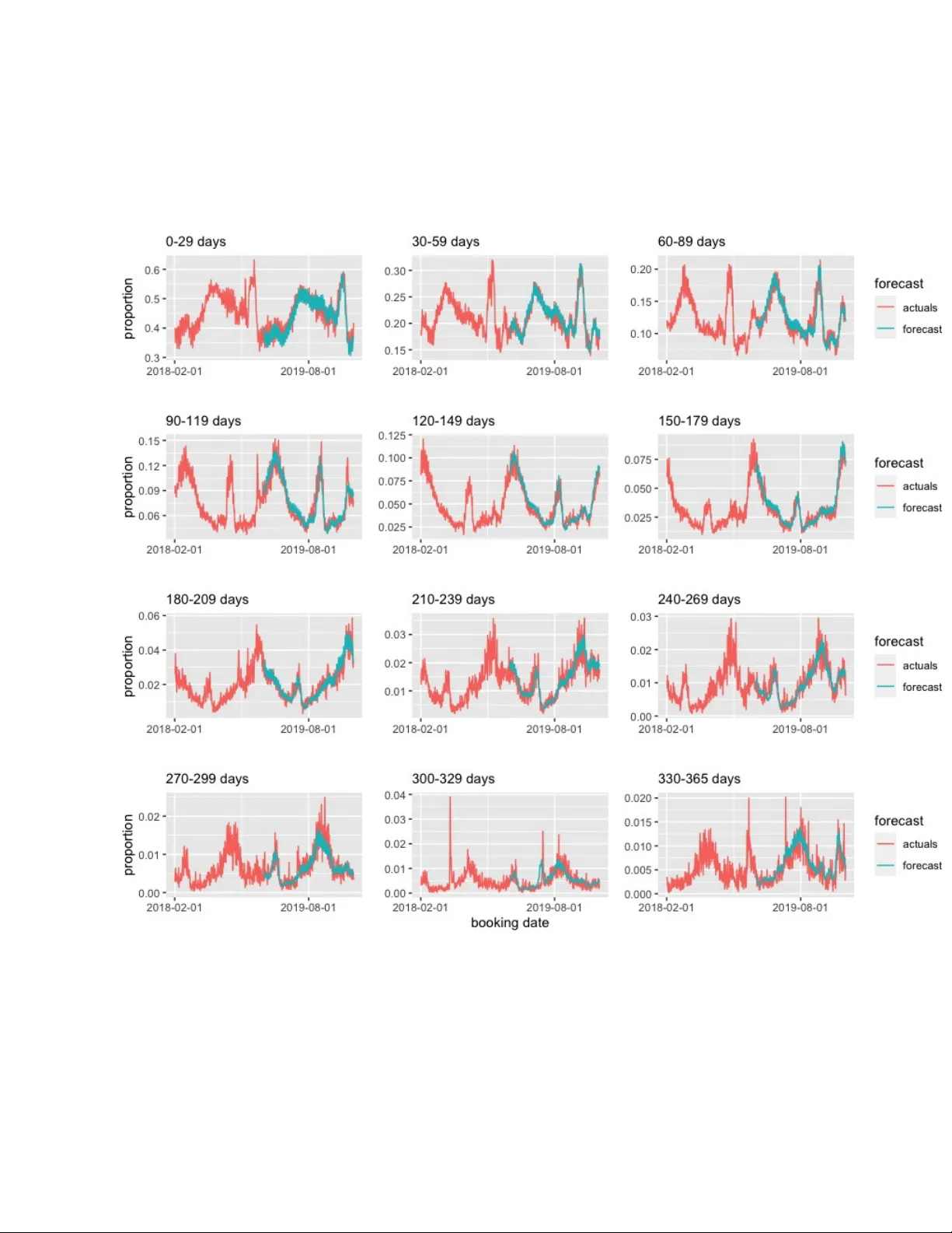
A Ba y esian Diric hlet Auto-Regressiv e Mo ving Av erage Mo del for F orecasting Lead Times Harrison Katz 1,2 , Kai Thomas Brusc h 2 , and Rob ert E. W eiss 3 1 Departmen t of Statistics, UCLA 2 Data Science, F orecasting, Airbnb 3 Departmen t of Biostatistics, UCLA Fielding Sc ho ol of Public Health Abstract In the hospitalit y industry , lead time data is a form of compositional data that is crucial for business planning, resource allocation, and staffing. Hospitality businesses accrue fees daily , but recognition of these fees is often deferred. This pap er presents a no vel class of Ba yesian time series mo dels, the Bay esian Diric hlet Auto-Regressive Mo ving Average (B-DARMA) mo del, designed specifically for comp ositional time se- ries. The mo del is motiv ated b y the analysis of five y ears of daily fees data from Airbn b, with the aim of forecasting the prop ortion of future fees that will b e recog- nized in 12 consecutiv e monthly interv als. Eac h da y’s comp ositional data is mo deled as Dirichlet distributed, giv en the mean and a scale parameter. The mean is mo deled using a V ector Auto-Regressive Mo ving Average pro cess, whic h dep ends on previous comp ositional data, previous comp ositional parameters, and daily co v ariates. The B-D ARMA mo del provides a robust solution for analyzing large comp ositional vec- tors and time series of v arying lengths. It offers efficiency gains through the c hoice of priors, yields in terpretable parameters for inference, and pro duces reasonable fore- casts. The pap er also explores the use of normal and horsesho e priors for the V AR and VMA co efficients, and for regression co efficien ts. The efficacy of the B-DARMA mo del is demonstrated through simulation studies and an analysis of Airbnb data. Keyw ords: Additive Log Ratio, Finance, Lead time, Simplex, Compositional data, Diric hlet distribution, Bay esian multiv ariate time series, Airbnb, V ector ARMA model, Mark ov Chain Mon te Carlo (MCMC), Hospitality Industry , Reven ue F orecasting, Generalized ARMA mo del 1 1 In tro duction T ra vel, entertainmen t, and hospitality businesses earn fees eac h da y , ho wev er these fees cannot b e recognized until later. The le ad time is the amoun t of time un til fees earned on a given da y can b e recognized. F uture dates that fees may b e recognized are allo cated into regular in terv als forming a partition of the future, often w eekly , monthly or annual time in terv als. Eac h da y , another vector of fee allo cations is observed. The distribution of fees in to future in terv als can b e analyzed separately from the total amount of fees; fractional allo cations in to future in terv als sum to one and form a comp ositional time series. The basic comp ositional observ ation is a contin uous vector of probabilities that a dollar earned to da y can b e recognized in each future interv al. W e wish to understand the process generating the comp ositional time series and forecast the series on in to the future. This information can b e used by businesses for the allo cation of resources, for business planning, and for staffing. W e analyze five y ears of daily fees billed at Airbn b that will b e recognized in the future. F uture fees are allo cated to one of 12 consecutiv e mon thly in terv als; fees b ey ond this range are small and ignored in this analysis. More gran ular inference on lead time of rev enue recognition would not improv e business planning or resource allo cation though it substantially complicates mo deling, mo del fitting, and communication of results. T o forecast a curren t day’s allo cations we ha v e all prior da ys’ data and we ha ve deterministic c haracteristics of days suc h as day of the week, season, and sequential da y of the y ear. A lead time comp ositional time series y t = ( y t 1 , . . . , y tJ ) ′ is a m ultiv ariate J -v ector time series with observ ed data y tj where t = 1 , . . . , T , indexes consecutiv e days or other time units, j = 1 , . . . , J indexes the J future reven ue recognition in terv als, 0 < y tj < 1 and P J j =1 y tj = 1 for all t . A natural mo del for comp ositional data is the Diric hlet distribution whic h is in the exp onential family of distributions and th us Dirichlet time series are sp ecial cases of generalized linear time series. Benjamin et al. (2003) prop osed a univ ariate Generalized ARMA data mo del in a frequentist framew ork. 2 There are numerous b o oks on Bay esian Analysis of Time Series Data (Barb er et al., 2011; Berliner, 1996; P ole et al., 2018; Ko op and Korobilis, 2010; W est, 1996; Prado and W est, 2010) as well as pap ers on Ba yesian v ector auto-regressive (AR) (V AR) moving a v erage (MA) (VMA) (ARMA)(V ARMA) time series mo dels (Sp encer, 1993; Uhlig, 1997; Ba ´ nbura et al., 2010; Karlsson, 2013); and on Ba yesian generalized linear time series mo dels (Brandt and Sandler, 2012; Rob erts and P enny, 2002; Nariswari and Pudjihastuti, 2019; Chen and Lee, 2016; McCab e and Martin, 2005; Berry and W est, 2020; Nariswari and Pudjihastuti, 2019; F ukumoto et al., 2019; Silv eira de Andrade et al., 2015; W est, 2013). Diric hlet time series data are less commonly mo deled in the literature. Grun wald et al. (1993) prop osed a Ba yesian compositional state space model with data mo deled as Diric hlet giv en a mean v ector, with the current mean giv en the prior mean also mo deled as Diric hlet. Grun w ald do es not use Marko v chain Monte Carlo (MCMC) for mo del fitting. Similarly , da Silv a et al. (2011) prop osed a state space Ba yesian mo del for a time series of prop ortions, extended in da Silv a and Ro drigues (2015) to Diric hlets with a static scale parameter. Zheng and Chen (2017) propose a frequentist Dirichlet ARMA time series. Muc h of the prior w ork on modeling comp ositional data and compositional time series transforms y t from the original J -dimensional simplex to a Euclidean space where the data is no w mo deled as normal (Aitchison, 1982; Cargnoni et al., 1997; Ra vishanker et al., 2001; Silv a and Smith, 2001; Mills, 2010; Barcelo-Vidal et al., 2011; Koehler et al., 2010; Kynˇ clo v´ a et al., 2015; Sn yder et al., 2017; AL-Dh urafi et al., 2018). It w ould seem preferable to not transform the raw data before modeling and instead mo del the data y t directly as Diric hlet distributed. Th us w e propose a new class of Ba yesian Diric hlet Auto-Regressiv e Moving Average mo dels (B-DARMA) for comp ositional time series. W e mo del the data as Dirichlet given the mean and scale, then transform the J -dimensional mean parameter vector to a J − 1-dimensional v ector. The distributional parameters are then mo deled with v ector auto-regressiv e mo ving a verage structure. W e also mo del the Dirichlet scale parameter as a log linear function of time-v arying predictors. W e giv e a general framew ork, and presen t submodels motiv ated b y our Airbn b lead time 3 data. The B-D ARMA mo del can b e applied to data sets with large comp ositional v ectors or few observ ations, offers efficiency gains through choice of priors and/or submo dels, and pro vides sensible forecasts on the Airbnb data. W e consider normal and horsesho e priors for the V AR and VMA co efficients, and for regression co efficients. Normal priors ha ve long b een a default for co efficients while the horsesho e is a newer choice whic h allows for v arying amounts of shrink age (Carv alho et al., 2009, 2010; Hub er and F eldkirc her, 2019; Kastner and Hub er, 2020; Ba ´ nbura et al., 2010) dep ending on the magnitude of the co efficien ts. The next section presents the B-D ARMA mo del. Section 3 presents simulation studies comparing the B-D ARMA to b oth a frequen tist DARMA data model and a transformed data normal V ARMA mo del. Section 4 presents analysis of the Airbnb data. The pap er closes with a short discussion. 2 A Ba y esian Diric hlet Auto-Regressiv e Mo ving Av- erage Mo del 2.1 Data mo del W e observe a J -comp onen t multiv ariate comp ositional time series y t = ( y t 1 , . . . , y tJ ) ′ , ob- serv ed at consecutive integer v alued times t = 1 up to the most recent time t = T , where 0 < y tj < 1, 1 ′ y t = 1 where 1 is a J − v ector of ones. W e mo del y t as Diric hlet with mean v ector µ µ µ t = ( µ t 1 , . . . , µ tJ ) ′ , with 0 < µ tj < 1, 1 ′ µ µ µ t = 1, and scale parameter ϕ t > 0 y t | µ µ µ t , ϕ t ∼ Diric hlet( ϕ t µ µ µ t ) , (1) with density f ( y t | µ µ µ t , ϕ t ) ∝ Q J j =1 y ϕ t µ tj − 1 tj . W e mo del µ µ µ t as a function of prior observ ations y 1 , . . . , y t − 1 , prior means µ µ µ 1 , . . . , µ µ µ t − 1 and kno wn co v ariates x x x t in a generalized linear model framework. As µ µ µ t and y are con- 4 strained, we mo del µ µ µ t after reducing dimension using the additive lo g r atio (alr) link η η η t ≡ alr( µ µ µ t ) =  log  µ t 1 µ tj ∗  , . . . , log  µ tJ µ tj ∗  (2) where j ∗ is a chosen reference comp onen t 1 ≤ j ∗ ≤ J , and the element of η η η t that w ould corresp ond to the j ∗ th element log( µ j ∗ /µ j ∗ ) = 0 is omitted. The line ar pr e dictor η η η t is a J − 1-v ector taking v alues in R J − 1 . Giv en η η η t , µ µ µ t is defined by the in verse of equation (2) where µ tj = exp( η tj ) / (1 + P J − 1 j =1 exp( η tj )) for j = 1 , . . . , J , j  = j ∗ and for j = j ∗ , η tj ∗ = 1 / (1 + P J − 1 j =1 exp( η tj )). W e mo del η η η t as a V ector Auto-Regressive Moving Average (V ARMA) pro cess η η η t = P X p =1 A A A p (alr( y t − p ) − X X X t − p β β β ) + Q X q =1 B B B q (alr( y t − q ) − η η η t − q ) + X X X t β β β (3) for t = m + 1 , . . . , T where m = max( P , Q ), A A A p and B B B q are ( J − 1) × ( J − 1) co efficient ma- trices of the resp ective V ector Auto-Regressive (V AR) and V ector Moving Av erage (VMA) terms, X X X t is a known ( J − 1) × r β matrix of deterministic cov ariates including an intercept, and including seasonal v ariables and trend as needed, and β β β is an r β × 1 v ector of regression co efficien ts. The form of an intercept in X X X t is the ( J − 1) × ( J − 1) iden tit y matrix I J − 1 as J − 1 columns in X X X t . Giv en an r 0 × 1 v ector of co v ariates x x x t for da y t , the simplest form of X X X t is X X X t = I J − 1 ⊗ x x x t and r β = ( J − 1) ∗ r 0 . The additiv e log ratio in (3) is a m ultiv ariate logit link and leads to elements of matrices A A A p and B B B q and v ector β β β that are log o dds ratios. Given η η η t , µ µ µ t giv es the exp ected allo cations of fees to comp onents. Scale parameter ϕ t is mo deled with log link as a function of an r γ -v ector of co v ariates z z z t , ϕ t = exp( z z z t γ γ γ ) , (4) where γ γ γ is an r γ -v ector of co efficients. In the situation of no cov ariates for ϕ t , log ϕ t = γ for all t . 5 Define the consecutive observ ations y a : b = ( y a , . . . , y b ) ′ for p ositive integers a < b . T o b e w ell defined, linear predictor (3) requires having m previous observ ations y ( t − m ):( t − 1) , and corresp onding linear predictors η η η t − m , . . . , η η η t − 1 . In computing p osteriors, we condition on the first m observ ations y 1: m whic h then do not contribute to the lik eliho o d. F or the corresp onding first m linear predictors, on the righ t hand side of (3), w e set η η η 1 , . . . , η η η m equal to alr( y 1 ) , . . . , alr( y m ) which effectively omits the VMA terms B B B l (alr( y t − l )) from (3) when t − l ≤ m . In con trast, in (3) the V AR terms and X X X t β β β are well defined for t = 1 , . . . , m . Define the C -v ector θ θ θ of all unknown parameters θ θ θ = ( A A A prs , B B B q rs , β β β ′ , γ γ γ ′ ) ′ , where r , s = 1 , . . . , J − 1 index all elemen ts of matrices A A A p and B B B q , p = 1 , . . . , P , q = 1 , . . . , Q and C = ( P + Q ) ∗ ( J − 1) 2 + r β + r γ . Prior b eliefs p ( θ θ θ ) ab out θ θ θ are up dated by Bay es’ theorem to give the p osterior p ( θ θ θ | y 1: T ) = p ( θ θ θ ) p ( y ( m +1): T | θ θ θ , y 1: m ) p ( y ( m +1): T | y 1: m ) , where p ( y ( m +1): T | θ θ θ , y 1: m ) = Q T t = m +1 p ( y t | θ θ θ , y ( t − m ):( t − 1) ), p ( y t | θ θ θ , y ( t − m ):( t − 1) ) is the densit y of the Dirichlet in (1), and the normalizing constan t p ( y ( m +1): T | y 1: m ) = R p ( θ θ θ ) p ( y ( m +1): T | θ θ θ , y 1: m ) d θ θ θ . W e wish to forecast the next S observ ations y ( T +1):( T + S ) . These hav e joint predictive dis- tribution p ( y ( T +1):( T + S ) | y 1: T ) = Z θ θ θ p ( y ( T +1):( T + S ) | θ θ θ ) p ( θ θ θ | y 1: T ) d θ θ θ . The join t predictive distribution p ( y ( T +1):( T + S ) | y 1: T ) can be summarized for example b y the mean or median against time t ∈ ( T + 1) : ( T + S ) to comm unicate results to business managers. Our data mo del can b e view ed as a Bay esian m ultiv ariate Diric hlet extension of the Generalized ARMA mo del by Benjamin et al. (2003). Similarly , Zheng and Chen (2017) prop ose a D ARMA data mo del whose link function in (2) do es not hav e an analytical in v erse, so needs to b e approximated n umerically . They view our data model as an ap- pro ximation to theirs, noting that the resulting noise sequence from having the analytical 6 in v erse isn’t a martingale difference sequence (MDS). This lack of an MDS complicates the in v estigation of the probabilistic properties of the series and the asymptotic b eha vior of their estimators. F rom a Bay esian persp ective, the need for an MDS for making inference is circum ven ted. Ba y esian inference is based on the p osterior distribution of the parameters, whic h com bines the likelihoo d function (dep enden t on the data) and the prior distribution (representing our prior b eliefs about the parameters). This allows us to make inferences regardless of whether the data form an MDS. F urthermore, the concept of a “noise sequence” or residuals is somewhat differen t in the con text of generalized linear mo dels (GLMs) compared to lo cation-scale mo dels lik e linear regression. In GLMs, residuals are not explicitly defined, and the noise sequence discussed in the con text of Zheng and Chen’s mo del is an approximation. In our Bay esian approach, w e do not need to define or consider the noise sequence at all, which simplifies the mo del and the analysis. 2.2 Choice of link function The link function in (2) and (3) can b e replaced with other common simplex transformations suc h as the Centered Log-Ratio (CLR) clr( y ) =  ln  y 1 g ( y )  , ln  y 2 g ( y )  , . . . , ln  y J g ( y )  where g ( y ) = ( y 1 × y 2 × . . . × y J ) 1 /J . Alternatively , the Isometric Log-Ratio (ILR) trans- formation can b e used, with j -th comp onen t y j = r r j r j + 1 log    g j ( y )  Q i ∈ H j y i  1 /r j    where g j ( y ) is the geometric mean of a subset S j of y , H j is the complement of S j , and r j is the num b er of elements in H j . The choice of subsets S j and H j can v ary dep ending on 7 the sp ecific problem and interpretation requiremen ts. Egozcue et al. (2003) show that the co efficien t matrices of the ALR, CLR, and ILR are linear transformations of each other. This means that the DARMA data mo dels with these three link functions are equiv alent, pro vided the same transformation is applied to the priors. 2.3 Mo del selection F or mo del selection, w e use the approximate calculation of the leav e-future-out (LF O) estimate of the exp ected log p oint wise predictiv e densit y (ELPD) for each mo del whic h measures predictive p erformance (Bernardo and Smith, 2009; V eh tari and Ojanen, 2012), ELPD LFO = T − M X t = L log p ( y ( t +1):( t + M ) | y 1: t ) where p ( y ( t +1):( t + M ) | y 1: t ) = Z θ θ θ p ( y ( t +1):( t + M ) | y 1: t , θ θ θ ) p ( θ θ θ | y 1: t ) d θ θ θ , (5) where M is the n umber of step ahead predictions and L is a c hosen minim um n umber of ob- serv ations from the time series needed to make predictions. W e use Monte-Carlo metho ds to appro ximate (5) with S ∗ random draws from the p osterior and estimate p ( y ( t +1):( t + M ) | y 1: t ) as p ( y ( t +1):( t + M ) | y 1: t ) ≈ 1 S ∗ S ∗ X s =1 p ( y ( t +1):( t + M ) | y 1: t , θ θ θ ( s ) 1: t ) for s = 1 , . . . , S ∗ dra ws from the p osterior distribution p ( θ θ θ | y 1: t ). Calculating the ELPD LF O requires refitting the mo del for eac h t ∈ ( L, . . . , T − M ), to get around this, we use approximate M-step ahead predictions using P areto smo othed imp ortance sampling (B ¨ urkner et al., 2020). 8 2.4 Priors A useful v ague prior for the individual co efficients in θ θ θ is a prop er indep enden t normal N ( V 0 , V ) with v arying V 0 ’s and V ’s dep ending on prior b eliefs ab out the co efficients. W e tak e V 0 = . 4 , . 1 in our data analysis when w e believe a priori that the co efficients will be p ositiv e and V 0 = 0 when we are unsure. F or elements a prs and b q rs of A A A p and B B B q matrices, w e tak e V = . 5 2 as we exp ect those elements to b e b etw een [ − 1 , 1]. F or elemen ts of β β β , w e migh t for example let V v ary with the standard deviation of the cov ariate. It ma y b e though t that man y elemen ts of θ θ θ migh t b e at or near zero. In this case, rather than a normal prior, w e might consider a shrink age prior lik e that proposed b y Carv alho et al. (2010), who prop ose a horsesho e prior of the form θ c | τ , λ c ∗ ∼ N (0 , τ 2 λ 2 c ∗ ) λ c ∗ ∼ C + (0 , 1) . for some c ∗ = 1 , . . . , C ∗ , c = 1 , . . . , C , and C ∗ ≤ C . Eac h θ c b elongs to one of c ∗ = 1 , . . . , C ∗ groups and eac h group gets its o wn shrink age parameter λ c ∗ applied to it. W e apply this with comp onent sp ecific shrink age parameters in our data analysis. 3 Sim ulation study In t wo sim ulation studies, w e study the B-D ARMA mo del’s capacity to accurately retrieve true parameter v alues, a critical asp ect for reliable forecasting. By comparing B-DARMA with established mo dels on a n umber of metrics, we pro vide a robust assessment of both its estimation and forecasting p oten tial. Eac h simulation study has L = 400 data sets indexed b y l = 1 , . . . , L with T = 540 observ ations y ( l ) t , t = 1 , . . . , T with J = 3 comp onen ts, j ∗ = 3 as the reference comp onen t for all mo dels, and Y Y Y l = ( y ( l ) 1 , . . . , y ( l ) T ). W e split the 540 observ ations into a training set of the first 500 observ ations and a test set of the last 40 observ ations, the holdout data, which the mo del is not trained on and whic h is used to 9 sho w the mo dels’ forecasting p erformance. In b oth studies, we compare B-D ARMA to a non-Bay esian DARMA data mo del and to a non-Bay esian transformed-data normal V ARMA (tV ARMA) mo del that transforms y ( l ) t to alr( y ( l ) t ) ∈ R J − 1 and mo dels alr( y t ) ∼ N J − 1 ( η η η t , Σ ), where Σ is an unknown J − 1 × J − 1 p ositiv e semi-definite matrix, and η η η t is defined in (3). W e use the V ARMA function from the MTS pac k age (Tsa y et al., 2022) in R (R Core T eam, 2022) to fit the tV ARMA mo dels with maxim um likelihoo d. F or the non-Ba yesian DARMA data mo del, the BF GS algorithm as implemen ted in optim in R is used for optimization. T o compute the parameters’ standard errors, the negative inv erse Hessian at the mo de is calculated. The data generating mo del (DGM) is a D ARMA mo del in simulation 1 and a tV ARMA mo del in sim ulation 2. W e set p = 1, q = 1 for a DARMA(1 , 1) (simulation 1) or tV ARMA(1 , 1) (sim ulation 2) data generating mo del. T o k eep the parameterization of the B-DARMA( P, Q ) model consisten t with the pa- rameterization of the MTS pack age, w e remo ve − X X X t − p β β β , p = 1 , . . . , P from the V AR term in (3) and set η η η t = P P p =1 A A A p (alr( y t − p )) + P Q q =1 B B B q (alr( y t − q ) − η η η t − q ) + X X X t β β β ∗ , where β β β ∗ = β β β − P P p =1 A A A p β β β and we drop the asterisk on β β β for the remainder of this section. All B-D ARMA mo dels are fit with ST AN (Stan Developmen t T eam, 2022) in R. W e run 4 chains with 2000 iterations each with a w arm up of 1000 iterations for a p osterior sample of 4000. Initial v alues are selected randomly from the interv al [ − 1 , 1]. In all sim ulations, the co v ariate matrix X X X t = I I I 2 , the 2 × 2 identit y matrix. Unknown co efficien t matrices A A A and B B B ha v e dimension 2 × 2. The shared parameters of in terest for the D ARMA, B-DARMA, and tV ARMA are β β β = ( β 1 , β 2 ) ′ , B B B = ( b rs ), and A A A p = ( a prs ) , r , s = 1 , 2, p = 1 and β β β = ( β 1 , β 2 ) ′ . W e use the out of sample F orecast Ro ot Mean Squared Error, FRMSE j , and F orecast Mean Absolute Error, FMAE j for each comp onen t j as a measure 10 of forecasting p erformance FRMSE j =  1 400   1 40  400 X l =1 540 X t =501 ( y l tj − ¯ µ l tj ) 2 ! 1 2 FMAE j =  1 400   1 40  400 X l =1 540 X t =501 | y l tj − ¯ µ l tj | where ¯ µ l tj is the p osterior mean of µ tj or the maxim um lik eliho o d estimate in the l th data set. The tV ARMA mo del has additional unknown co v ariance matrix Σ Σ Σ = (Σ rs ) , r , s = 1 , 2 a function of 3 unkno wn parameters, t wo standard deviations σ 1 = Σ 1 / 2 11 , σ 2 = Σ 1 / 2 22 , and correlation ρ = Σ 12 / ( σ 1 ∗ σ 2 ), while the B-DARMA and DARMA hav e a single unknown scale parameter ϕ . F or the tV ARMA data generating sim ulations w e set σ 1 = σ 2 = . 05, ρ = . 30, and for DARMA generating mo dels, we set ϕ = 1000. Priors in simulations 1 and 2 for the B-D ARMA(1 , 1) are indep endent N (0 , . 5 2 ) for all co efficien ts in β , A, B , and a priori γ = log ϕ ∼ Gamma(25 / 7 , 5 / 7) with mean 5 and v ariance 7. F or each parameter, generically θ , with true v alue θ true in sim ulation l , for Ba y esian mo dels we take the p osterior mean ¯ θ l as the p oin t estimate. F or the 95% Credible Interv al (CI) ( θ l low , θ l upp ) we tak e the endp oints to b e 2.5% and 97.5% quantiles of the p osterior. F or the tV ARMA and DARMA mo dels, w e use the maxim um lik eliho o d estimates (MLE) as the parameter estimate, and 95% confidence in terv als (CI) calculated as maxim um likelihoo d estimate plus or min us 1.96 standard errors. F or each parameter θ in turn, for the B-DARMA, tV ARMA, and DARMA mo dels, we assess bias, ro ot mean squared error (RMSE), length of the 95% CI (CIL), and the fraction 11 of simulations % IN where θ true falls within the 95% CI bias = 1 400 400 X l =1 ( ¯ θ l − θ true ) RMSE = 1 400 400 X l =1 ( ¯ θ l − θ true ) 2 ! 1 / 2 CIL = 1 400 400 X l =1  θ l upp − θ l low  % IN = 1 400 400 X l =1 1 { θ l low ≤ θ true ≤ θ l upp } for the B-D ARMA mo dels and replace ¯ θ l with the MLE for the tV ARMA and D ARMA mo dels. F or all sim ulations, elemen ts of β β β , A A A, B B B are set to b e β 1 = − 0 . 07 , β 2 = 0 . 10 , a 11 = 0 . 95 , a 12 = − 0 . 18 , a 21 = 0 . 3 , a 22 = 0 . 95 , b 11 = 0 . 65 , b 12 = 0 . 15 , b 21 = 0 . 2 , b 22 = 0 . 65 . 3.1 Comparing B-D ARMA, D ARMA, and tV ARMA Mo dels in sim ulations 1-2 Supplemen tary tables 4 and 5 pro vide summarized parameter reco v ery results, while table 1 gives the FRMSE j and FMAE j for each comp onen t. When the data generating mo del is a DARMA(1,1), B-DARMA consisten tly outp erforms tV ARMA, with the B-D ARMA(1,1) yielding an RMSE av eraging at 40% smaller, esp ecially for the B B B matrix co efficients. The B-D ARMA’s p erformance aligns with that of the frequentist D ARMA, eac h excelling in half of the ten considered co efficien ts. Both DARMA mo dels sho wcase co verage sup erior to the tV ARMA. F or a tV ARMA(1,1) data generating mo del, the tV ARMA generally exhibits the small- 12 est RMSE for all co efficien ts, barring b 11 . The difference in RMSE is marginal, a veraging at 2%. The B-DARMA and frequentist DARMA compare similarly for β β β and A A A , but the D ARMA p erforms w orse for B B B . B-D ARMA has b etter cov erage than b oth tV ARMA and frequen tist DARMA for most co efficients excepting β 2 , b 21 , and b 22 . The out-of-sample prediction results are summarized in table 1. When the DGM is a D ARMA(1,1), the B-D ARMA outp erforms both the frequen tist D ARMA model and the tV ARMA in FRMSE and FMAE across all comp onen ts, most notably for y 3 . When the DGM is a tV ARMA, for y 1 and y 2 the B-DARMA p erforms comparably to the tV ARMA and outp erforms the D ARMA. F or y 3 , the B-DARMA significantly outp erforms b oth the tV ARMA and DARMA. 4 Airbn b Lead Time Data Analysis The Airbn b lead time data, y t , is a comp ositional time series for a specific single large mark et where each comp onent is the prop ortion of fees b o oked on da y t that are to b e recognized in 11 consecutive 30 day windo ws and 1 last consecutiv e 35 da y windo w to co v er 365 days of lead times. Figures 1 and 2 plot the Airbn b lead time data from 01/01/2015 to 01/31/2019 and 03/26/2015 to 05/14/2015 resp ectively . There is a distinct rep eated y early shap e in figure 1 and a clear weekly seasonality in figure 2. Figure 1 shows a gradual increase/decrease in comp onen t sizes, most notably a decrease for the first window of [0 , 29) da ys. The levels are driven by the attractiv eness of certain tra vel p erio ds with guests b o oking earlier and pa ying more for p eak p erio ds lik e summer and the December holiday season. The weekly v ariation sho ws a pronounced contrast b et ween weekda ys and w eek ends. Thus we wan t to include weekly and y early seasonal v ariables and a trend v ariable in the predictors X X X t in (3). W e model eac h component with its o wn linear trend and use F ourier terms for our seasonal v ariables, pairs of  sin 2 k π t w season , cos 2 k π t w season  for k = 1 , . . . , K season ≤ w season 2 where w e tak e w season = w week = 7 for w eekly seasonality and w season = w year = 365 . 25 for y early 13 seasonalit y . The orthogonality of the F ourier terms helps with con v ergence whic h is why w e prefer it to other seasonal representations. W e train the mo del on data from 01/01/2015 to 1/31/2019, choose a forecast window of 365, and use 02/01/2019 to 01/31/2020 as the test set. All B-DARMA mo dels are fit with ST AN using the R in terface where we run 4 c hains with 3000 iterations each with a w arm up of 1500 iterations for a total of 6000 p osterior samples. Initial v alues are selected randomly from the in terv al [ − 1 , 1]. 4.1 Mo del W e use the appro ximate LF O ELPD of candidate mo dels to first decide on the n umber of yearly F ourier terms, K year giv en initial c hoices of P and Q , then given the n umber of F ourier terms we decide on the orders P and Q . W e fix K season = K week = 3, the pairs of F ourier terms for mo deling w eekly seasonality , for all mo dels. W e use an intercept and the same seasonal v ariables and linear trend for ϕ t . T o define LFO ELPD, we tak e the step ahead predictions to b e M = 1, the minimum n um b er of observ ations from the time series to make predictions to b e L = 365, and the threshold for the Pareto estimates to b e . 7 (B ¨ urkner et al., 2020; V eh tari et al., 2015) which resulted in needing to refit mo dels at most 12 times. F or all of the mo del selection pro cess, w e set indep endent N (0 , . 5 2 ) priors for eac h ( a prs ) , r , s = 1 , . . . , 11 , p = 1 , 2 and ( b q rs ) , r , s = 1 , . . . , 11 , q = 1, indep enden t N (0 , 1) priors on the F ourier co efficien ts, N (0 , . 1) priors on the linear trend co efficients, and a N (0 , 4) prior on the intercepts. W e use these same priors for the seasonal, intercept and trend co efficien ts in γ in (4). W e fixed P = 1, Q = 0 and let K season = K year tak e on increasing v alues starting with 3 then sequen tially K year = 6 , 8 , 9 , 10 with increasing v alues of LF O ELPD un til 10 had w orse LF O ELPD, so we stopp ed and to ok K year = 9 (table 2). W e fixed K year = 9 and similarly to ok ( P , Q ) = (1 , 0) first then ( P, Q ) = (1 , 1) and ( P , Q ) = (2 , 0) with (1 , 0) p erforming b est (table 2). 14 W e compare four differen t B-DAR(1) mo dels plus a DAR(1) mo del and a tV AR(1) mo del. Mo del 1 (Horsesho e F ull) has a horsesho e ( τ = 1) prior on the co efficients in β β β and γ γ γ with a separate shrink age parameter λ c ∗ for the elements of θ θ θ that corresp ond to each η j or to ϕ . As w e exp ect the AR a rs elemen ts to diminish in magnitude as the time difference | r − s | increases, the other three mo dels hav e v arying prior mean and sd for a rs as functions of | r − s | . Mo del 2 (Normal F ull) has an a rr ∼ N ( . 4 , . 5 2 ) prior on its diagonal elements r = 1 , . . . , 11, a a r ( r +1) , a r ( r − 1) ∼ N ( . 1 , . 5 2 ) prior on its t w o nearest neighbors, r = 1 , . . . , 10 and r = 2 , . . . , 11 respectively and a N (0 , . 5 2 ) prior on the remaining elemen ts of the A A A matrix. In contrast to mo dels 1 and 2, where all parameters a rs in A A A are allo wed to v ary , models 3 and 4 fix some of the parameters a rs to 0. Mo del 3 (Normal Nearest Neighbor) only allows a r ( r +1) , r = 1 , . . . , 10 , a r ( r − 1) , r = 2 , . . . , 11 and a rr , r = 1 , 2 , . . . , 11 to v ary and mo del 4 (Normal Diagonal) only allo ws a rr , r = 1 , 2 , . . . , 11 to v ary . The remaining elemen ts in mo del 3 a r ( r + k ) for k ≥ 2 or k ≤ − 2 in the A A A matrix are set equal to 0. F or mo del 4 all off diagonal elemen ts, a rs r  = s , are set to 0. The non-zero co efficien ts hav e the same priors as the Normal F ull. All 3 Normal mo dels ha ve the same priors on coefficients γ γ γ and β β β : N (0 , 1) and N (0 , . 1 2 ) for the co efficien ts of the F ourier and trend terms resp ectively . The scale mo del predictors include the same seasonal and trend terms and the corresp onding priors on the co efficients are the same as for the η η η ’s. The prior on the intercepts in β β β and γ γ γ is N (0 , 2 2 ). Mo del 5 (D AR(1)) is the frequentist counterpart to our B-DAR(1) Normal F ull mo del with the same seasonal and trend terms for η j and ϕ . Mo del 6 (tV AR(1)) is a frequentist transformed V AR mo del which models alr( y t ) ∼ N J − 1 ( η η η t , Σ ). It has the same seasonal and trend v ariables in η η η t . Both mo dels 5 and 6 are fit in R, mo del 5 with the BFGS algorithm as implemented in optim and mo del 6 with the V ARX function in the MTS pack age. 15 4.2 Results In the training set, the Horsesho e F ull mo del has the largest LF O ELPD (supplemen tary table 8). The LF O ELPD for the Normal F ull mo del and the Normal Nearest Neigh b or mo del are close to the Horsesho e F ull mo del with the Normal Diagonal mo del ha ving a m uc h w orse LF O ELPD than the other mo dels. F or the test set, the F orecast Ro ot Mean Squared Error (FRMSE j ) and the F orecast Mean Absolute Error (FMAE j ) for each comp onent is in table 3 as well as the total F ore- cast Ro ot Mean Squared Error and F orecast Mean Absolute Error for eac h mo del. The Normal F ull mo del p erforms b est on the test set for most comp onen ts and has the low est total F orecast Ro ot Mean Squared Error and smallest total F orecast Mean Absolute Error, with the Horseshoe F ull mo del about 1 . 5% and . 1% w orse resp ectiv ely . The differences b et w een the tw o full mo dels (Mo del 1 and 2) and Mo dels 3 and 4 are largest for the larger comp onen ts as the FRMSE’s for the smaller comp onents are closer. F or example, for the largest comp onen t y 1 , the Normal Diagonal mo del performs o ver 7% w orse than the Normal F ull mo del. The Normal Nearest Neighbor mo del p erforms w ell considering it has 91 fewer parameters than the Normal F ull model, p erforming 3% w orse in total than the Normal F ull mo del. When compared to the frequentist models, the Normal F ull mo dels exhibit sup erior p erformance in the largest comp onen ts y 1 and y 2 , ha ving a smaller FMAE and a smaller FRMSE j . F or the smaller comp onen ts y 4 through y 12 , the differences in FRMSE j among the models are subtler, although the FMAE v alues con tin ue to show a more pronounced difference across all comp onents. The D AR(1) do es p erform b etter than the subsetted B-D AR(1) mo dels with a total FRMSE roughly 2 . 5% smaller than the Normal Nearest- Neigh b or mo del and 5% less than the Normal Diagonal mo del. The tV AR(1) p erforms significan tly worse than all the DAR mo dels, with a total FRMSE ab out 15% larger than the w orst p erforming D AR data mo del, suggesting the time in v arian t nature of Σ Σ Σ is inap- propriate for the data. Figures 3 and 4 plot out of sample forecasts ( ¯ µ tj ) and residuals of (alr( y t ) − ˆ η η η t ) for the 16 Normal F ull model. The mo del captures most of the y early seasonality and the residual terms exhibit no consisten t p ositive or negative bias for any of the comp onents as they are all cen tered near 0. Much of the remaining residual structure may b e explained b y market sp ecific holidays whic h are not incorp orated in the curren t mo del. The estimated yearly and w eekly seasonality for eac h of the η η η j ’s (ALR scale) and ϕ (log scale) in the Normal F ull mo del are detailed in supplemen tary figures 5 and 6. Y early v ari- ation is pronounced in larger comp onents, with η η η 1 p eaking in late December and troughing b efore the new y ear, while ϕ exhibits a simpler pattern with t w o high and one lo w p erio d. W eekly seasonalit y displays a consisten t weekda y versus w eek end b ehavior across all η η η j comp onen ts, sho wing higher v alues on week ends. Supplemen tary table 9 summarizes the p osterior statistics for the in tercepts and linear gro wth rates of η η η j s and log( ϕ ), showing a monotonic decrease in the intercepts and larger growth rates for smaller comp onents. The gro wth rate of ϕ indicates less comp ositional v ariabilit y ov er time. Lastly , the p osterior densities for the elements a rs of the A A A matrix, shown in supplementary figure 7, reveal that larger comp onents ha ve pronounced co efficients on their own lag, a rr , with diminishing magnitude for distant trip dates, while smaller components exhibit more uncertaint y but generally maintain a strong p ositive co efficient on their own lag. 5 Discussion There are distinct differences in the computational costs in fitting our D ARMA mo del using frequen tist or Bay esian metho dologies, as well as the tV ARMA mo del using the MTS pac k age in R. Firstly , fitting the tV ARMA mo del using the MTS pack age was fastest, attributable to its implementation of conditional maxim um lik eliho o d estimation with a m ultiv ariate Gaussian likelihoo d. This approac h b enefits from the mathematical simplicity of estimation under the normal model and its unconstrained optimization problem, resulting in significan tly less computational o v erhead. This is in addition to the built-in p erformance optimizations found in sp ecialized pack ages lik e MTS. 17 In con trast, the Ba yesian D ARMA model, implemen ted using Hamiltonian Mon te Carlo (HMC), had higher computational costs. This is to b e exp ected, giv en that HMC requires running many iterations to generate a representativ e sequence of samples from the p oste- rior distribution. How ev er, the B-DARMA fit faster than the frequentist D ARMA. The frequen tist DARMA mo del, fitted using the Bro yden–Fletc her–Goldfarb–Shanno (BFGS) optimization method, w as the most computationally demanding in our study . The com- plexit y arises from the calculation of the Hessian matrix estimates, the computation of gamma functions in the Dirichlet lik eliho o d, and the constraint of p ositive parameters. Notably , around 25% of mo del fitting attempts in the simulation studies initially failed and required regenerating data and refitting the mo del, underscoring the computational c hallenges of this approac h. This pap er presented a new class of Ba y esian comp ositional time series mo dels assum- ing a Dirichlet conditional distribution of the observ ations, with time v arying Diric hlet parameters whic h are mo deled with a V ARMA structure. The B-DARMA outp erforms the frequentist tV ARMA and DARMA when the underlying data generating mo del is a D ARMA and do es comparably w ell to the tV ARMA and outp erforms the DARMA when tV ARMA is the data generating mo del in the sim ulation studies. By choice of prior and mo del subsets, w e can reduce the n um b er of co efficien ts needing to b e estimated and b etter handle data sets with few er observ ations. This class of mo dels effectiv ely mo dels the fee lead time b eha vior at Airbn b, outp erforming the DAR and tV AR with the same co v ariates, and provides an in terpretable, flexible framework. F urther dev elopment is p ossible. Common comp ositional time series hav e comp onents with no ordering while the 12 lead time comp onen ts in the Airbn b data set are time ordered. This suggests θ θ θ can b e mo deled hierarchically . The construction of the Nearest Neighbor and Diagonal mo dels for A A A 1 are examples of using time ordering in mo del specification. While the distributional parameters µ µ µ t and ϕ t are time-v arying, the elements of θ θ θ are static and th us the seasonalit y is constan t ov er time, which may not b e appropriate for other data sets. W e mo del ϕ t with exogenous cov ariates, but our approac h is flexible enough to 18 allo w for it to hav e a more complex AR structure itself. While not an issue for the Airbn b data set, the mo del’s inabilit y to handle 0’s would need to b e addressed for data sets with exact zero es. Ac kno wledgemen t The authors thank Sean Wilson, Jac kson W ang, Peter Coles, T om F ehring, Jenn y Cheng, Erica Sav age, and George Roumeliotis for helpful discussions. The authors would also like to thank the Editor, the Asso ciate Editor, and three anonymous reviewers for their careful reading, comments, and suggestions to an earlier version of the pap er. Sp ecial thanks are extended to Emily Liv ely , Lauren Mack evich, and Stephanie Ch u for their indisp ensable supp ort in navigating administrative, programmatic, and legal asp ects, resp ectively , which significan tly contributed to the timely completion and dissemination of this pap er. Co de and Data Av ailabilit y The primary dataset used in our study , “A Ba yesian Diric hlet Auto-Regressive Mo ving Av erage Mo del for F orecasting Lead Times,” is not publicly av ailable due to confidentialit y constrain ts. How ever, the Stan co de for the Bay esian Diric hlet Auto-Regressive Mo ving Av erage (B-D ARMA) mo del is av ailable for public access. It can b e found at our GitHub rep ository: https://gith ub.com/harrisonek atz/B-D ARMA-pap er. References Aitc hison, J. (1982). The statistical analysis of comp ositional data. Journal of the R oyal Statistic al So ciety: Series B (Metho dolo gic al) 44 (2), 139–160. AL-Dh urafi, N. A., N. Masseran, and Z. H. Zamzuri (2018). Comp ositional time series 19 analysis for air p ollution index data. Sto chastic Envir onmental R ese ar ch and Risk As- sessment 32 (10), 2903–2911. Ba ´ nbura, M., D. Giannone, and L. Reic hlin (2010). Large Ba y esian v ector auto regressions. Journal of Applie d Ec onometrics 25 (1), 71–92. Barb er, D., A. T. Cemgil, and S. Chiappa (2011). Bayesian Time Series Mo dels . Cambridge Univ ersit y Press. Barcelo-Vidal, C., L. Aguilar, and J. A. Mart ´ ın-F ern´ andez (2011). Comp ositional v arima time series. Comp ositional Data Analysis: The ory and Applic ations , 87–101. Benjamin, M. A., R. A. Rigby , and D. M. Stasinop oulos (2003). Generalized autoregressiv e mo ving a verage mo dels. Journal of the Americ an Statistic al asso ciation 98 (461), 214– 223. Berliner, L. M. (1996). Hierarchical Ba y esian time series mo dels. In Maximum Entr opy and Bayesian Metho ds , pp. 15–22. Springer. Bernardo, J. M. and A. F. Smith (2009). Bayesian the ory , V olume 405. John Wiley & Sons. Berry , L. R. and M. W est (2020). Bay esian forecasting of many coun t-v alued time series. Journal of Business & Ec onomic Statistics 38 (4), 872–887. Brandt, P . T. and T. Sandler (2012). A Ba yesian Poisson vector autoregression mo del. Politic al Analysis 20 (3), 292–315. B ¨ urkner, P .-C., J. Gabry , and A. V eh tari (2020). Approximate leav e-future-out cross- v alidation for Ba y esian time series mo dels. Journal of Statistic al Computation and Sim- ulation 90 (14), 2499–2523. Cargnoni, C., P . M ¨ uller, and M. W est (1997). Ba yesian forecasting of multinomial time se- ries through conditionally Gaussian dynamic models. Journal of the A meric an Statistic al Asso ciation 92 , 640–647. 20 Carv alho, C. M., N. G. P olson, and J. G. Scott (2009). Handling sparsity via the horse- sho e. In Pr o c e e dings of the Twelth International Confer enc e on Artificial Intel ligenc e and Statistics , pp. 73–80. Pro ceedings of Mac hine Learning Research 5. Carv alho, C. M., N. G. P olson, and J. G. Scott (2010). The horsesho e estimator for sparse signals. Biometrika 97 (2), 465–480. Chen, C. W. and S. Lee (2016). Generalized Poisson autoregressiv e mo dels for time series of counts. Computational Statistics & Data A nalysis 99 , 51–67. da Silv a, C. Q., H. S. Migon, and L. T. Correia (2011). Dynamic Bay esian beta mo dels. Computational Statistics & Data A nalysis 55 (6), 2074–2089. da Silv a, C. Q. and G. S. Ro drigues (2015). Ba y esian dynamic Dirichlet mo dels. Commu- nic ations in Statistics-Simulation and Computation 44 (3), 787–818. Egozcue, J. J., V. P a wlo wsky-Glahn, G. Mateu-Figueras, and C. Barcelo-Vidal (2003). Isometric logratio transformations for comp ositional data analysis. Mathematic al ge ol- o gy 35 (3), 279–300. F ukumoto, K., A. Beger, and W. H. Mo ore (2019). Bay esian modeling for o verdispersed ev en t-count time series. Behaviormetrika 46 (2), 435–452. Grun w ald, G. K., A. E. Raftery , and P . Guttorp (1993). Time series of contin uous prop or- tions. Journal of the R oyal Statistic al So ciety: Series B (Metho dolo gic al) 55 (1), 103–116. Hub er, F. and M. F eldkircher (2019). Adaptiv e shrink age in Bay esian vector autoregressiv e mo dels. Journal of Business & Ec onomic Statistics 37 (1), 27–39. Karlsson, S. (2013). F orecasting with Bay esian v ector autoregression. Handb o ok of Ec o- nomic F or e c asting 2 , 791–897. Kastner, G. and F. Hub er (2020). Sparse Bay esian v ector autoregressions in h uge dimen- sions. Journal of F or e c asting 39 (7), 1142–1165. 21 Ko ehler, A. B., R. D. Snyder, J. K. Ord, A. Beaumont, et al. (2010). F orecasting com- p ositional time series with exp onential smo othing metho ds. T ec hnical rep ort, Monash Univ ersit y , Department of Econometrics and Business Statistics. Ko op, G. and D. Korobilis (2010). Bayesian Multivariate Time Series Metho ds for Empir- ic al Macr o e c onomics . No w Publishers Inc. Kyn ˇ clov´ a, P ., P . Filzmoser, and K. Hron (2015). Mo deling comp ositional time series with v ector autoregressive mo dels. Journal of F or e c asting 34 (4), 303–314. McCab e, B. P . and G. M. Martin (2005). Bay esian predictions of lo w count time series. International Journal of F or e c asting 21 (2), 315–330. Mills, T. C. (2010). F orecasting comp ositional time series. Quality & Quantity 44 (4), 673–690. Narisw ari, R. and H. Pudjihastuti (2019). Ba y esian forecasting for time series of count data. Pr o c e dia Computer Scienc e 157 , 427–435. P ole, A., M. W est, and J. Harrison (2018). Applie d Bayesian for e c asting and time series analysis . Chapman and Hall/CRC. Prado, R. and M. W est (2010). Time series: mo deling, c omputation, and infer enc e . Chap- man and Hall/CRC. R Core T eam (2022). R: A L anguage and Envir onment for Statistic al Computing . Vienna, Austria: R F oundation for Statistical Computing. Ra vishank er, N., D. K. Dey , and M. Iy engar (2001). Comp ositional time series analysis of mortality prop ortions. Communic ations in Statistics-The ory and Metho ds 30 (11), 2281–2291. Rob erts, S. J. and W. D. P enn y (2002). V ariational Ba yes for generalized autoregressive mo dels. IEEE T r ansactions on Signal Pr o c essing 50 (9), 2245–2257. 22 Silv a, D. and T. Smith (2001). Mo delling comp ositional time series from rep eated surv eys. Survey Metho dolo gy 27 (2), 205–215. Silv eira de Andrade, B., M. G. Andrade, and R. S. Ehlers (2015). Bay esian garma mo dels for coun t data. Communic ations in Statistics: Case Studies, Data Analysis and Appli- c ations 1 (4), 192–205. Sn yder, R. D., J. K. Ord, A. B. Ko ehler, K. R. McLaren, and A. N. Beaumon t (2017). F orecasting comp ositional time series: A state space approach. International Journal of F or e c asting 33 (2), 502–512. Sp encer, D. E. (1993). Dev eloping a Bay esian vector autoregression forecasting mo del. International Journal of F or e c asting 9 (3), 407–421. Stan Developmen t T eam (2022). RStan: the R in terface to Stan. R pack age version 2.21.5. Tsa y , R. S., D. W o o d, and J. Lac hmann (2022). MTS: Al l-Purp ose T o olkit for Analyz- ing Multivariate Time Series (MTS) and Estimating Multivariate V olatility Mo dels . R pac k age version 1.2.1. Uhlig, H. (1997). Ba y esian vector autoregressions with sto chastic v olatility . Ec onometric a: Journal of the Ec onometric So ciety , 59–73. V eh tari, A. and J. Ojanen (2012). A surv ey of Bay esian predictive metho ds for mo del assessmen t, selection and comparison. Statistics Surveys 6 , 142–228. V eh tari, A., D. Simpson, A. Gelman, Y. Y ao, and J. Gabry (2015). P areto smo othed imp ortance sampling. arXiv pr eprint arXiv:1507.02646 . W est, M. (1996). Ba y esian time series: Mo dels and computations for the analysis of time series in the physical sciences. In Maximum Entr opy and Bayesian Metho ds , pp. 23–34. Springer. W est, M. (2013). Ba y esian dynamic mo delling. Bayesian Infer enc e and Markov Chain Monte Carlo: In Honour of A drian FM Smith , 145–166. 23 Zheng, T. and R. Chen (2017). Diric hlet ARMA mo dels for comp ositional time series. Journal of Multivariate Analysis 158 , 31–46. Figures and tables DGM: D ARMA(1,1) tV ARMA(1,1) Mo del: B-D ARMA DARMA tV ARMA B-D ARMA DARMA tV ARMA FRMSE y 1 0.1054 0.1091 0.1063 0.0566 0.0794 0.0566 y 2 0.1342 0.1367 0.1356 0.0748 0.0775 0.0748 y 3 0.1015 0.1082 0.1470 0.0548 0.0640 0.0787 FMAE y 1 0.0770 0.0777 0.0800 0.0432 0.0633 0.0432 y 2 0.1004 0.1009 0.1020 0.0574 0.0652 0.0574 y 3 0.0766 0.0775 0.1102 0.0422 0.0529 0.0617 T able 1: Sim ulation study F orecast Ro ot Mean Squared Error (FRMSE) and F orecast Mean Absolute Error (FMAE) on the test set ( T = 40). DGM is data generating mo del. Sim ulation study 1 is on the left and study 2 on the right. (P ,Q) pairs of F ourier terms ELPD diff LFO ELPD (1,0) 9 0.0 70135.3 (1,0) 10 -23.3 70112.0 (1,0) 8 -83.2 70052.0 (1,0) 6 -594.7 69540.6 (1,0) 3 -1190.1 68945.2 (1,1) 9 -101.7 70033.6 (2,0) 9 -123.7 70011.5 T able 2: Airbnb data analysis - Lea ve-future-out exp ected log p oin t wise predictiv e densit y (LF O ELPD) and the LFO ELPD differences b et ween the b est p erforming B-D ARMA mo del and candidate B-D ARMA mo dels. The first fiv e candidate mo dels fix ( P , Q ) and v ary pairs of F ourier terms for y early seasonality and the last tw o candidate mo dels fix the F ourier terms at 9 pairs and v ary ( P , Q ). 24 Normal Horsesho e Normal Normal F ull F ull Nearest-Neighbor Diagonal DAR(1) tV AR(1) FRMSE y 1 0.0211 0.0213 0.0216 0.0225 0.0213 0.0301 y 2 0.0122 0.0124 0.0129 0.0132 0.0124 0.0145 y 3 0.0101 0.0101 0.0103 0.0106 0.0101 0.0118 y 4 0.0094 0.0094 0.0097 0.0099 0.0094 0.0110 y 5 0.0061 0.0061 0.0062 0.0063 0.0061 0.0076 y 6 0.0050 0.0050 0.0051 0.0052 0.0050 0.0056 y 7 0.0037 0.0037 0.0039 0.0040 0.0037 0.0042 y 8 0.0029 0.0029 0.0030 0.0031 0.0029 0.0033 y 9 0.0023 0.0023 0.0023 0.0023 0.0023 0.0026 y 10 0.0022 0.0022 0.0023 0.0023 0.0022 0.0023 y 11 0.0025 0.0023 0.0025 0.0025 0.0025 0.0025 y 12 0.0022 0.0022 0.0022 0.0022 0.0022 0.0030 T otal 0.0796 0.0800 0.0821 0.0841 0.0801 0.0983 FMAE y 1 0.0170 0.0171 0.0174 0.0181 0.0172 0.0247 y 2 0.0090 0.0094 0.0099 0.0111 0.0096 0.0113 y 3 0.0076 0.0079 0.0081 0.0083 0.0079 0.0090 y 4 0.0067 0.0068 0.0070 0.0079 0.0070 0.0085 y 5 0.0048 0.0049 0.0049 0.0051 0.0049 0.0059 y 6 0.0039 0.0039 0.0042 0.0042 0.0039 0.0044 y 7 0.0027 0.0027 0.0027 0.0030 0.0027 0.0032 y 8 0.0021 0.0021 0.0022 0.0023 0.0022 0.0025 y 9 0.0018 0.0018 0.0018 0.0019 0.0018 0.0019 y 10 0.0016 0.0016 0.0016 0.0016 0.0016 0.0017 y 11 0.0017 0.0017 0.0017 0.0017 0.0017 0.0018 y 12 0.0016 0.0016 0.0016 0.0017 0.0016 0.0022 T otal 0.0605 0.0615 0.0631 0.0669 0.0621 0.0771 T able 3: Airbnb data analysis - F orecast Ro ot Mean Squared Error (FRMSE) and F orecast Mean Absolute Error (FMAE) for the 12 comp onen ts and their total for the test set from F eb 1, 2019 to Jan 31, 2020. 25 Figure 1: Airbn b data analysis - prop ortion of fees b y lead time for a single large market from Jan 1, 2015 to Jan 31, 2019. 26 Figure 2: Airbn b data analysis- Prop ortion of fees for a single large mark et: weekly seasonal b eha vior. 27 Figure 3: Airbnb data analysis - Normal F ull Model: one y ear of predictions (blue) from F eb 1, 2019 to Jan 31, 2020 and tw o y ears of actuals (red) for each of the 12 comp onen ts. 28 Figure 4: Airbnb data analysis - Normal full mo del residuals on the additiv e log ratio scale, η η η t − ˆ η η η t , for the test set, F eb 1, 2019 to Jan 31, 2020. 29 par mo del true RMSE bias cov erage length β 1 B-D ARMA -.07 0.0083 -0.0019 0.9450 0.0312 D ARMA 0.0088 -0.0015 0.9225 0.0312 tV ARMA 0.0112 -0.0038 0.9000 0.0354 β 2 B-D ARMA .10 0.0081 -0.0012 0.9425 0.0313 D ARMA 0.0083 -0.0007 0.9425 0.0312 tV ARMA 0.0096 -0.0035 0.9425 0.0361 a 11 B-D ARMA .95 0.0113 -0.0021 0.9250 0.0385 D ARMA 0.0108 -0.0025 0.9600 0.0395 tV ARMA 0.0145 -0.0036 0.8950 0.0428 a 12 B-D ARMA -.18 0.0074 -0.0014 0.9400 0.0287 D ARMA 0.0079 -0.0009 0.9400 0.0294 tV ARMA 0.0133 -0.0013 0.8500 0.0316 a 21 B-D ARMA .30 0.0101 -0.0020 0.9500 0.0373 D ARMA 0.0101 -0.0009 0.9500 0.0382 tV ARMA 0.0127 -0.0041 0.9225 0.0436 a 22 B-D ARMA .95 0.0086 -0.0021 0.9300 0.0311 D ARMA 0.0084 -0.0018 0.9300 0.0316 tV ARMA 0.0108 -0.0028 0.9050 0.0323 b 11 B-D ARMA .65 0.0309 -0.0064 0.9450 0.1244 D ARMA 0.0308 -0.0011 0.9500 0.1286 tV ARMA 0.1012 -0.0759 0.5025 0.1593 b 21 B-D ARMA .20 0.0314 0.0003 0.9475 0.1168 D ARMA 0.0297 0.0018 0.9425 0.1162 tV ARMA 0.0907 -0.0485 0.5650 0.1768 b 12 B-D ARMA .15 0.0286 0.0010 0.9525 0.1145 D ARMA 0.0289 0.0031 0.9525 0.1139 tV ARMA 0.0900 -0.0514 0.5425 0.1645 b 22 B-D ARMA .65 0.0321 -0.0040 0.9500 0.1283 D ARMA 0.0341 0.0013 0.9350 0.1272 tV ARMA 0.1135 -0.0868 0.4550 0.1575 Supplemen tary T able 4: Sim ulation study 1 results (RMSE, bias, co verage and length of the 95% credible or confidence interv al) for B-DARMA(1,1) tV ARMA(1,1) and DARMA(1,1) when the data generating mo del is a DARMA(1,1) for the tw o regression co efficien ts in β β β , the four a rs elemen ts of the A matrix, and four b rs elemen ts of the B matrix. 30 par mo del true RMSE bias cov erage length β 1 B-D ARMA -.07 0.0063 -0.0012 0.9650 0.0254 D ARMA 0.0065 -0.0008 0.9275 0.0336 tV ARMA 0.0061 -0.0013 0.9450 0.0238 β 2 B-D ARMA .10 0.0069 -0.0010 0.9625 0.0254 D ARMA 0.0065 -0.0007 0.9400 0.0334 tV ARMA 0.0062 -0.0010 0.9550 0.0241 a 11 B-D ARMA .95 0.0125 -0.0035 0.9525 0.0461 D ARMA 0.0125 -0.0038 0.9300 0.0604 tV ARMA 0.0115 -0.0022 0.9525 0.0431 a 12 B-D ARMA -.18 0.0086 -0.0004 0.9650 0.0344 D ARMA 0.0091 -0.0007 0.9225 0.0595 tV ARMA 0.0084 -0.0007 0.9600 0.0321 a 21 B-D ARMA .30 0.0115 -0.0010 0.9600 0.0454 D ARMA 0.0112 -0.0009 0.9375 0.0453 tV ARMA 0.0111 -0.0007 0.9500 0.0437 a 22 B-D ARMA .95 0.0090 -0.0025 0.9475 0.0347 D ARMA 0.0096 -0.0040 0.9275 0.0456 tV ARMA 0.0086 -0.0016 0.9450 0.0325 b 11 B-D ARMA .65 0.0342 -0.0050 0.9475 0.1320 D ARMA 0.0365 -0.0015 0.9300 0.1728 tV ARMA 0.0348 0.0002 0.9350 0.1287 b 21 B-D ARMA .20 0.0342 -0.0027 0.9275 0.1318 D ARMA 0.0357 0.0032 0.9150 0.1718 tV ARMA 0.0337 -0.0007 0.9475 0.1315 b 12 B-D ARMA .15 0.0325 -0.0011 0.9600 0.1320 D ARMA 0.0346 -0.0005 0.9125 0.1707 tV ARMA 0.0319 0.0012 0.9475 0.1278 b 22 B-D ARMA .65 0.0354 -0.0077 0.9375 0.1317 D ARMA 0.0366 0.0003 0.8850 0.1717 tV ARMA 0.0344 -0.0008 0.9475 0.1318 Supplemen tary T able 5: Sim ulation study 2 results (RMSE, bias, co verage and length of the 95% credible or confidence in terv al) for B-D ARMA(1,1), tV ARMA(1,1) and D ARMA(1,1) when the data generating mo del is a tV ARMA(1,1) for the t w o regression co efficien ts in β β β , the four a rs elemen ts of the A matrix, and four b rs elemen ts of the B matrix. 31 P arameter Mo del Net Bias RMSE Ratio Net Co v erage Length Ratio β 1 D ARMA -0.0004 1.06 -0.0225 1.00 tV ARMA -0.0019 1.35 -0.0450 1.13 β 2 D ARMA 0.0005 1.02 0.0000 0.99 tV ARMA -0.0023 1.18 0.0000 1.15 a 11 D ARMA -0.0004 0.96 0.0350 1.03 tV ARMA -0.0015 1.28 -0.0300 1.11 a 12 D ARMA 0.0005 1.07 0.0000 1.02 tV ARMA 0.0001 1.80 -0.0900 1.10 a 21 D ARMA 0.0011 1.00 0.0000 1.02 tV ARMA -0.0021 1.26 -0.0275 1.17 a 22 D ARMA 0.0003 0.98 0.0000 1.02 tV ARMA -0.0007 1.26 -0.0250 1.04 b 11 D ARMA 0.0053 1.00 0.0050 1.03 tV ARMA -0.0695 3.27 -0.4425 1.28 b 21 D ARMA 0.0006 0.95 -0.0050 0.99 tV ARMA -0.0482 2.89 -0.3825 1.51 b 12 D ARMA 0.0001 1.01 0.0000 0.99 tV ARMA -0.0504 3.15 -0.4100 1.44 b 22 D ARMA 0.0073 1.06 -0.0150 0.99 tV ARMA -0.0828 3.54 -0.4950 1.23 Supplemen tary T able 6: Simulation study 1 results (Net Bias, RMSE Ratio, Net Cov- erage, and Credible/Confidence Interv al Length Ratio) comparing B-D ARMA(1,1) with tV ARMA(1,1) and DARMA(1,1) when the data generating mo del is a DARMA(1,1) for the tw o regression co efficients in β β β , the four a rs elemen ts of the A matrix, and four b rs ele- men ts of the B matrix. RMSE and Length ratios greater than 1 and negative net co verage differences fav or the B-D ARMA mo del. 32 P arameter Mo del Net Bias RMSE Ratio Net Co v erage Length Ratio β 1 D ARMA -0.0004 1.03 -0.0375 1.32 tV ARMA -0.0001 0.97 -0.0200 0.94 β 2 D ARMA 0.0003 0.94 -0.0225 1.31 tV ARMA 0.0000 0.90 -0.0075 0.95 a 11 D ARMA -0.0003 1.00 -0.0225 1.31 tV ARMA 0.0013 0.92 0.0000 0.93 a 12 D ARMA -0.0003 1.06 -0.0425 1.73 tV ARMA -0.0003 0.98 -0.0050 0.93 a 21 D ARMA 0.0001 0.97 -0.0225 1.00 tV ARMA 0.0003 0.97 -0.0100 0.96 a 22 D ARMA -0.0015 1.07 -0.0200 1.31 tV ARMA 0.0009 0.96 -0.0025 0.94 b 11 D ARMA 0.0035 1.07 -0.0175 1.31 tV ARMA 0.0052 1.02 -0.0125 0.98 b 21 D ARMA 0.0059 1.04 -0.0125 1.30 tV ARMA 0.0020 0.98 0.0200 1.00 b 12 D ARMA 0.0006 1.06 -0.0475 1.29 tV ARMA 0.0023 0.98 -0.0125 0.97 b 22 D ARMA 0.0080 1.03 -0.0525 1.30 tV ARMA 0.0069 0.97 0.0100 1.00 Supplemen tary T able 7: Sim ulation study 2 results (Net Bias, RMSE Ratio, Net Cov erage, and Length Ratio) comparing B-D ARMA(1,1) with tV ARMA(1,1) and D ARMA(1,1) when the data generating mo del is a tV ARMA(1,1) for the tw o regression co efficients in β β β , the four a rs elemen ts of the A matrix, and four b rs elemen ts of the B matrix. RMSE and Length ratios greater than 1 and negative net co verage differences fa vor the B-D ARMA mo del. mo del ELPD diff LFO ELPD Horsesho e F ull 0.0 70149.2 Normal F ull -8.9 70140.3 Normal Nearest-Neighbor -37.3 70112.0 Normal Diagonal -186.2 69963.1 Supplemen tary T able 8: Airbnb data analysis - Lea v e-future-out expected log point wise predictiv e density (LF O ELPD) and the LFO ELPD differences b etw een the b est p erform- ing B-DARMA mo del and candidate B-D ARMA mo dels. 33 par Mean SD Q2.5 Q97.5 η 1 in tercept -0.228 0.055 -0.337 -0.121 η 2 -0.526 0.071 -0.666 -0.389 η 3 -0.719 0.091 -0.897 -0.545 η 4 -1.033 0.112 -1.254 -0.811 η 5 -1.483 0.136 -1.750 -1.215 η 6 -2.409 0.169 -2.740 -2.070 η 7 -2.791 0.209 -3.200 -2.384 η 8 -2.819 0.249 -3.299 -2.330 η 9 -2.999 0.301 -3.592 -2.417 η 10 -3.064 0.349 -3.743 -2.380 η 11 -4.879 0.354 -5.572 -4.176 ϕ 6.746 0.023 6.701 6.791 η 1 linear growth 0.238 0.080 0.085 0.395 η 2 0.607 0.100 0.411 0.804 η 3 0.778 0.125 0.533 1.024 η 4 1.104 0.154 0.800 1.402 η 5 1.674 0.189 1.306 2.050 η 6 2.235 0.239 1.766 2.702 η 7 2.669 0.304 2.077 3.268 η 8 2.627 0.366 1.905 3.341 η 9 2.404 0.449 1.529 3.285 η 10 3.547 0.520 2.531 4.564 η 11 7.297 0.512 6.295 8.314 ϕ 6.824 0.268 6.297 7.347 Supplemen tary T able 9: Airbn b data analysis - summary coefficients for the normal full mo del. Parameter (par), p osterior mean (Mean), standard deviation (SD), and 95 % CI. The linear growth rates are m ultiplied b y 10 4 . 34 Supplemen tary Figure 5: Airbn b data analysis - plot of the p osterior mean yearly seasonal v ariation of the 11 comp onents on the ALR scale and of the y early seasonal v ariation for ϕ on the log scale for the normal full mo del Jan 1, 2015 to Jan 31, 2019. 35 Supplemen tary Figure 6: Airbnb data analysis - plot of the p osterior mean w eekly season- alit y ( η ALR scale, ϕ log scale) for the normal full mo del. 36 0.0 0.2 0.4 0.6 1 2 3 4 5 6 7 8 9 10 11 s a rs r=1 0.0 0.2 0.4 1 2 3 4 5 6 7 8 9 10 11 s r=2 0.0 0.1 0.2 0.3 0.4 0.5 1 2 3 4 5 6 7 8 9 10 11 s r=3 0.0 0.1 0.2 0.3 0.4 1 2 3 4 5 6 7 8 9 10 11 s a rs r=4 0.0 0.1 0.2 0.3 0.4 1 2 3 4 5 6 7 8 9 10 11 s r=5 -0.1 0.0 0.1 0.2 1 2 3 4 5 6 7 8 9 10 11 s r=6 -0.1 0.0 0.1 0.2 0.3 1 2 3 4 5 6 7 8 9 10 11 s a rs r=7 -0.1 0.0 0.1 0.2 0.3 1 2 3 4 5 6 7 8 9 10 11 s r=8 -0.2 0.0 0.2 1 2 3 4 5 6 7 8 9 10 11 s r=9 -0.4 -0.2 0.0 0.2 0.4 1 2 3 4 5 6 7 8 9 10 11 s a rs r=10 -0.4 -0.2 0.0 0.2 1 2 3 4 5 6 7 8 9 10 11 s r=11 Supplemen tary Figure 7: Airbnb data analysis - p osterior density of elements a rs in V AR A 1 matrix. The cen ter p oin t of each densit y plot is the median of the p osterior distribution and line segments are 95% credible in terv als. 37