Prediction, Communication, and Computing Duration Optimization for VR Video Streaming

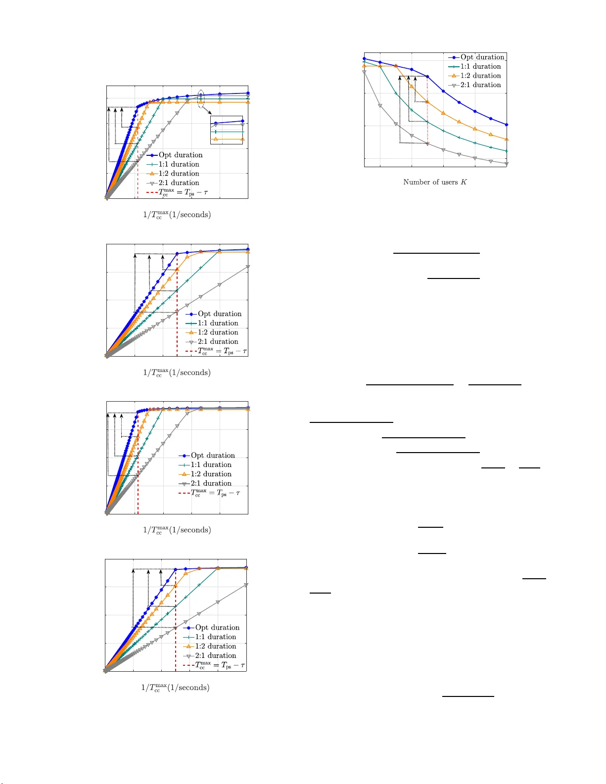
1 Prediction, Communication, and Computing Duration Optimization for VR V ideo Streaming Xing W ei, Chenyang Y ang, and Shengqian Han Abstract —Proacti ve tile-based video stream ing can av oid motion-to-photon latency of wireless virtual reality (VR) by computing and delivering the predicted tiles to be requested befor e playback. All existing works either f ocus on designing pre- dictors or allocating computing and communications resources. Y et to av oid the latency , the successively executed pre diction, communication, and computing tasks should be accomplished within a predetermined time. More ov er , th e quality of experi- ence (QoE) of proacti ve VR streaming depen ds on th e worst perfo rmance of the three tasks. In thi s paper , we jointly op t imize the duration of the o bserva tion wi ndow fo r predicting tiles and the durations for computing an d transmitti ng the predicted til es, aimed at b alancing the performa nce for three tasks to maximize the QoE giv en arbitrary predictor and configured resour ces. W e obtain the closed-f orm optimal solution by decomposing the fo rmulated problem equivalently into two sub p roblems. With the optimized durations, we find a resour ce-limited r egion where the QoE in creases rapidly with configured resour ces, and a prediction-limited region where the QoE can be i mp ro ved more efficiently with a better predictor . S imulation results using th ree existing predictors and a real dataset validate the analysis and demonstrate the gain from the joint optimization over non- optimized counterparts. Index T erms —Wireless VR, proacti ve tiled-based VR vid eo streaming, p rediction, computing, communication. I . I N T RO D U C T I O N W ireless v irtual reality (VR) ca n p rovide an immersive ex- perience to wireless users. As the main typ e of VR services [ 1], VR v ideo usually has 360 ◦ × 180 ◦ panora m ic view w ith ultra high resolution (e. g. 1 6 K [2]). Evidently , deli vering such video is cost-pro hibitiv e for wireless networks. However , the range of ang les that h umans can see a t the same time is only a limited area of the full panora m ic view (abou t 110 ◦ × 90 ◦ [3]), called field of view (FoV). This inspires tile-based strea m ing [4], [5], which di vides a full pano ramic view segment into small tiles in spatial do main, and only co m putes and tran smits the tiles overlapped with th e FoVs. T o avoid dizziness in watching VR video, the motion-to- photon ( MTP) latency should b e low , which usually sho uld be less than 20 m s [6]. With reactive tile-based streaming, the tiles within the FoVs sho u ld be computed an d delivered within the MTP latency after a user initiates a requ est, which demand s for very high transmission rate an d computing rate [6], [7]. Proacti ve tile-based streaming can a void the MTP This work was supported by National Natural Science Foundat ion of China (NSFC) under Grant 61671036, Grant 61871015, and Grant 61731002. Xing W ei, Chenyan g Y ang, and Shengqian H an are with the School of Electronics and Information Engineering, Beiha ng Uni versit y , Beijing 100191, China , Shengqian Han is also with the Hang zhou Innov ation Institute, Beihan g Unive rsity , Hangzhou 310000, China (e-mail: weixing@buaa .edu.cn, cyya ng@bua a.edu.cn, sqhan@buaa .edu.cn). latency [5], [6], [ 8 ], w h ich is anticipated to be th e mainstream in the ultimate stage of VR video streaming [6 ]. A. Motivation an d Major Con tributions Proactive tile-based VR video streaming contains three tasks: pr e diction, c o mmunica tio n, and co mputing . Before the playback of a segment, the tiles to be most likely reque sted in the segment are first p r edicted using the user b ehavior -related data in an ob servation win dow , wh ich are then comp uted and finally delivered to the user . T o avoid the MTP latency , these successively executed tasks should be acco mplished within a pr e-determin ed duration, which de p ends on the “ c oherence time” of th e u ser-behavior related data in watching a VR video , th e employed p redictor and th e playb a c k duration o f a segment. On the other h a n d, even without the MTP latency , the quality of exper ience (QoE) of a user may degrad e d ue to the b lack ho le s during VR video playback [5], [ 9]. This occurs when the following cases happen. (1) More tiles to be requested in a segment ca n be corr ectly predicted with longer observation window , but no enough time is left for computin g and d eli vering all the pred icted tiles before the playback of th e segment. (2 ) Mo re tiles can be compute d an d delivered with longer time for compu ting an d co mmunicatio n, but some of th e se tiles are not requ ested due to the poor prediction p erforma n ce. It sug gests that the Qo E de p ends on the worst perform ance of th e three tasks. I n this context, the perf ormance of p rediction indicates how many tiles to be requested can be pred icted corr ectly [ 8], [10], and the perfor mance of commun ication and computing refers to how many pred icted tiles can be computed and delivered befo re playback . The pr e diction p erform ance is restricted by the “coheren ce time” e ven with th e best predictor . Delivering an d computin g large a m ount of data within shor t time req u ires high transmission and co mputing rates. T o m a ximize th e QoE with a giv en pr e dictor and configu red resourc e s, the performan ce of the three tasks should be balanced. This can be achieved by judiciously allocating the d urations fo r the o bservation window and fo r pro cessing and d eli vering the p redicted tiles. In this paper , we striv e to in vestigate h ow to match the computin g ra te an d tra n smission rate to the prediction perfor- mance to m aximize the QoE o f proactive tile-based VR v id eo streaming. The main con tributions are summarized as follows. • T o balance the perfo r mance of the thre e tasks, we for- mulate a pr oblem to optim ize the duration assigned to the o bservation win dow for any given p redictor a nd the duration s for pro cessing and de li vering th e p redicted tiles with given computin g an d transmission rates. 2 • W e find the optimal dur ations with c lo sed-form ex- pressions, with a reasonable assumptio n on the re latio n between the p rediction per f ormance an d the o bservation time, which is v alidated using existing pr edictors and a real dataset. From the optimal solution, we figure ou t a single p arameter to reflect th e configure d c ommunic a tio n and co mputing resour ces, and find r esource-limited and prediction -limited r egions, which provides usef u l in sights into the system design . In the resource- lim ited region, the QoE can be impr oved by bo osting commu nication and computin g perfo rmance. In the p rediction- limited region, the QoE c a n be imp roved mo r e effectiv ely by enhan c in g the pre d iction perfo rmance. B. Related W orks As far as the autho rs k nown, there are no prior works to co-design th e pred iction, comm unication, and co mputing tasks for p roactive tile-based VR vid eo streaming. For tile pred iction, a linear regression (LR) method was propo sed in [8] to pred ict the central poin t of FoV , which was then tra n sformed into correspo n ding tiles [11]. A deep r ein- forcemen t lear n ing techniqu e was used in [12] to pred ict the FoV of the next fr ame. A deep lear ning meth od was propo sed in [ 10] that uses he ad mou nted display (HM D ) orientation s, image saliency maps, an d m otion maps to p redict the tiles to be requested. Con text bandits (CB) lear ning te c h nique was considered in [11] to predict the tile requ ests and in [13] to predict th e user orientation in lon gitude and latitude. A sequence-to -sequence pred iction method was prop osed in [14] to p redict the futur e FoV in secon ds ahead . For commu nication and comp uting resource allocatio n, the renderin g task in co mputing was offloaded in [15] fr o m HMD to multiple-acce ss ed ge com puting (MEC) server to reduce the bandwid th usage an d com p utational workload on HMD. T he co mputing an d cachin g resour ces were le veraged in [16] to r educe th e c o mmunicatio n reso u rce usag e. Multicast oppor tunity was exploited for mu ltip le users watching the same v ideo in [1 7] to minim ize the transmission energy . The uplink and downlink comm unication reso u rce allocation was optimized in [18] to maximize a utility fun ction that takes prediction accu racy , co m munication delay , and comp uting delay into consideratio n. In [ 19], [20], partial c o mputing task was offloaded fro m the MEC ser ver to the HMD, wh ich reveals the trad eoff b etween caching and computing without considerin g tile prediction. I n our pre vious work [1 1], the duration s for comm unication and co mputing wer e o ptimized, while the dur ation for prediction was simply g i ven. All pr io r works d o not inv estigate h ow to balanc e the perfor mance of the thr ee tasks in order to max imize the QoE of pr oactive tile-based VR streamin g . The r e st of th is pap er is o rganized as follows. Section II describes th e sy stem m odel. Sec tio n III form ulates the problem , and Section IV derives the optimal solution and provides th e prediction -limited and resource- limited region s. Simulation and nu merical results are pr ovided in Section V to validate the assum ption, show th e QoE in the two r egions, and evaluate the gain from o ptimizing the duration s f o r three tasks. Sectio n VI conclu des the pape r . I I . S Y S T E M M O D E L Consider a pro activ e tile-b ased VR video streamin g system with an MEC server co-located with a base statio n (BS). Each VR v id eo consists o f L segments in tem poral domain , and each segment co nsists of M tiles in spatial do main. Th e playb ack duration of e a ch tile equals to the p layback dur ation of a segment, deno te d by T seg [5], [8]. Each user is equipp ed with a HMD, which can measure data 1 of the user, send the recorde d data to the MEC server, and p re-buffer segments. While both the MEC server and th e HMD can be u sed for rende ring, we consider that the MEC server rend ers a video segmen t befo re delivering to the HMD. VR vide o playback Communica tion pipeline t l+ 1 l+ 1 obw t cpt t Computing pipeline l+ 1 com t Head movement trace cc t b t ps T e t pdw seg T T = Predicted tiles l l l l Fig. 1: Proactively stream in g the ( l +1 )th segment of a VR video. t b is the start tim e for streamin g th e ( l +1 )th segment, and t e is the start time of p layback of the ( l +1)th segment. During the VR video playbac k, su b sequent segments are predicted, co mputed, and delivered on e after another [ 5], [6], as shown in Fig. 1 . Each segment has its own dead line for the prediction , co mputing, and communic a tion, hence the three tasks fo r L segments can be dec o upled into L g roups of task s. In the sequel, we take the ( l + 1 )th segment as an examp le for elaboration . W ith proactive VR streaming , the MTP latency can be av o id ed by pro cessing and delivering the tiles in the ( l +1 )th segment to be requested b efore t e . Hence, the tiles to be p la y ed in a pre d iction win dow , whic h begins at t e and is with du ration T p dw = T seg , sho uld be predic te d . This can be acc o mplished by first pr edicting the hea d move- ment sequence in th e predictio n wind ow with the observations (say also a head movement sequence ) in a time win dow with duration t obw , then ma p ping the pr edicted sequence into the predicted tiles [1 1], [22]. Since the prediction perfo rmance fo r a time series depend s on its a uto-corr elation, there exists a time instant t b , bef ore wh ich th e observations have low correlation with th e sequ ence to be predicted and hence co ntribute little or ev en negativ ely for imp roving th e pr e diction accu racy [ 10], 1 The useful data for prediction include sensor-rel ated data (i.e., the head mov ement orienta tion tracking [8] and eye tracking data [12], [21] from the HMD sensors), and content -relate d data (i.e., the images in historical FoVs [12], [22] and temporal-spatia l salienc y [10], [23]). The audio data in a VR video are also under discussion [23 ]. While our framework is applicable for pre dicti on using one or multiple types of data , we take the head move ment trace as an example for easy exposi tion. 3 [24], [25]. W e can set t b as the start time o f th e ob servation window . At the end of the observation window , the MEC server first makes the prediction, then renders the p r edicted tiles with dura tion t cpt , and finally deliv ers the processed tiles with d uration t com . Th en, the duratio n b etween t b and t e , denoted as T ps , is the total proactive stre a ming time av ailab le for p rediction, co m puting, and communicatio n, i.e., t obw + t cpt + t com ≤ T ps . Th e value of T ps can be prede ter- mined for any giv en dataset and pre d ictor [10], [ 24], [25]. The duration T ps + T p dw can b e regarded as the “coheren ce time” for th e head movement tim e series. A. Computing Mod el For tile-ba sed VR v ideo stream ing, re n dering contain s two steps. (1) Th e tiles in a segment are unpacked and the tiled- frames at the same timestamp are co ncatenated to generate successiv e two-dimen sional (2D) FoVs [ 15]. (2 ) The 2 D planar FoVs are converted to th e three-dim e n sional (3D) sp herical FoVs, by m ultiplying th e image matr ix of 2D FoV with a projection matrix (this step is sometimes c a lled “pro jection” in the r endering op eration [5]). I n p ractice, GPU is n ecessary for real-time renderin g. When the GPU with T ur ing arch itecture [26] is used for MEC [27], [ 28], th e com puting resou rce for renderin g a VR video can be assigne d by allocating co m pute unified d evice architec tu re cores [2 9] and m ultiple GPUs can be used at the ser ver . T o gain useful insight, we assume that the comp uting resource, d enoted as C total (in floatin g-poin t op e r ations per second, FLOPS), is equally allocated among K users. Then, the n umber of b its th at can b e ren dered per second , refer red to a s the computin g rate for the k th user, is C cpt ,k , C r,k µ r ( in b its/s ) , (1) where C r,k = C total /K is the co mputing resour ce assigned to the k th user for renderin g, an d µ r = T r C r γ fov R w R h b is th e required floating -point o perations (FLOPs) of rend ering one bit of FoV in FLOPs/bit , T r is the time used for rend ering a FoV , γ fov is the ratio of FoV in a frame, R w and R h are respectively the pixels in wide an d high of a fr ame, and b is the number of bits p er p ixel relevant to color depth [30]. B. T ransmission Model The BS equipp ed with N t antennas serves K sing le-antenna users with zero -forcin g beamformin g. The instantaneo us trans- mission rate at the i th time slot for th e k th user is C i com ,k = B log 2 1 + p i k d − α k | ˜ h i k | 2 σ 2 ! , (2) where B is the b a n dwidth, ˜ h i k , ( h i k ) H w i k is th e eq uiv alen t channel gain , p i k and w i k are r espectively the tr ansmit power and beamf orming vector for the k th u ser , d k and h i k ∈ C N t are respectively the distance and the small scale ch annel vector from the BS to the k th u ser, α is the path- loss exponent, σ 2 is the no ise power , an d ( · ) H denotes conju gate transpose. W e con sider indo or users as in the literatur e of wireless VR video streaming, where th e d istan ces of users usually chan ge slightly [2 2], [31], [3 2] and are assumed fixed. W e consider time-varying small-scale channels, which ar e assumed as remaining constant in each time slot with dur ation ∆ T and changin g amo ng time slots indep endently with identical dis- tribution. W ith the pro activ e transmission, the pred icted tiles in a segment should be transmitted with duration t com . The number o f b its transmitted within t com is C com ,k t com , wh ere C com ,k is the time-average rate in t com . When t com ≫ ∆ T , C com ,k = 1 N s P N s i =1 C i com ,k , where N s is the n umber of time slots in t com . Since fu ture ch a nnel is unknown when makin g the optimization , we use ensemble-average rate E h { C com ,k } to approx imate time-average rate C com ,k , where E h {·} is th e expectation over h , which is very accurate when N s or N t /K is large as v alidated v ia extensiv e simulation s. T o ensure fairness am o ng u sers in term s of QoE, the transmit power is a llocated to co mpensate th e path loss, i.e., p i k = β d − α k , where β can be o btained f rom β ( P K k =1 1 d − α k ) = P and P is the maximal tran smit power of the BS. Th e n, th e ensemble - av erage transmission rate f o r each user is eq ual. In the sequel, we first consider o n e user f or analysis and then show the impact o f K . W e u se C com to r eplace E h { C i com ,k } and u se C cpt to r eplace C cpt ,k for n otational simplicity . I I I . P RO B L E M F O R M U L AT I O N F O R O P T I M I Z I N G T H E D U R A T IO N S F O R T H R E E T A S K S In this section, we first introdu ce the perf o rmance metric s for the tile prediction task, for th e co m puting and commun i- cation tasks, and for the QoE in watching a VR video. T o balance the perfor mance of th e three tasks for maximizing the Qo E, we then formulate a p roblem to jointly o ptimize th e duration of the ob servation window with any given p redictor, and the duration s for commu nication and com puting with giv en comp u ting r ate an d transmission rate. A. P erformance Metric of T ile Pr ediction Degree of overlap (DoO) has been used to measur e the overlap between th e p redicted and the requested fr ames o f a pan oramic video [1 2], [31]. A larger value of DoO indicates a better predictio n. T o re flec t the prediction perform ance for proactive tile-based streaming, we consider se gment DoO (se g- DoO) , wh ich m e asures the overlap of th e pred icted tiles and the r equested tiles in a segment. Fro m this perspective, the DoO used in [1 2], [31] c a n be co nsidered as a special c ase of seg-DoO wher e a segment contains only one f r ame [31]. The seg-DoO of the l th segmen t is d e fined as DoO seg l ( t obw ) , q T l · p l ( t obw ) k q l k 1 , where q l , [ q l, 1 , ..., q l,M ] T denotes th e gr ound- tr uth of the tile reque sts for th e segment with q l,m ∈ { 0 , 1 } , e l ( t obw ) , [ e l, 1 ( t obw ) , ..., e l,M ( t obw )] T denotes the predicte d tile requ ests for the segment with e l,m ( t obw ) ∈ { 0 , 1 } , ( · ) T denotes 4 transpose of a vector, and k · k 1 denotes the ℓ 1 norm of a vector . When the m th tile in the l th segment is truly requested, q l,m = 1 , o th erwise q l,m = 0 . When the tile is predicted to be requested, e l,m ( t obw ) = 1 , other wise it is zero. W e use average seg-DoO to measure the p rediction perfo r- mance f or a VR v ideo, which is D ( t obw ) , 1 L L X l =1 DoO seg l ( t obw ) = ∞ X n =0 a n t n obw , (3) where the secon d eq u ality is the power series expan sion, which holds for any infinitely d ifferentiable function. The value of a n depend s o n the pred ictor . For any pre-d etermined value of T ps , a predictor can be more accurate with a longer ob servation window , b ecause th e tiles to b e pred icted are closer to and hence are more co rrelated with the head movement seq uence having been observed, as shown in Fig. 1. This gives rise to a reason able assumption as follows. Assumption 1 : D ( t obw ) is a mo notonically increasing fu nc- tion of t obw . B. Completion Rate of Communicatio n an d Comp uting T asks T o reflec t the perfo rmance of the sy stem fo r renderin g an d delivering the pre dicted tiles in a segment, we define th e completion rate of com munication and co mputing (CC) tasks as S cc ( t com , t cpt ) , min { S ( t com , t cpt ) , N } N , (4) where N , k e l ( t obw ) k 1 is the number o f p redicted tiles in a segment, S ( t com , t cpt ) is the num b er o f tiles in the segment that can be deliv ered with t com and compu ted with t cpt , w h ich is S ( t com , t cpt ) , min  C com t com s com , C cpt t cpt s cpt  , (5) where s com = r w r h bN tf /γ c [30] is the numb er o f bits in each tile fo r transmission , s cpt = r w r h bN tf is the numb e r of bits in a tile for renderin g, r w and r h are th e p ixels in wid e and high o f a tiled-fram e, γ c is the compr e ssion ra tio , and N tf is the number of tiled-fram e in a tile. After substituting (5) into (4), the completion rate of CC tasks can be expressed as S cc ( t com , t cpt ) = min  C com t com s com N , C cpt t cpt s cpt N , 1  . (6) C. Metric of Qua lity of Exp erience For proactive tile-based stream ing, there will be no MTP latency if the constraint t obw + t com + t cpt ≤ T ps can be satisfied. Y et black holes will appear if either th e requested tiles cann ot be p redicted corr e ctly , or some pr edicted tiles cannot b e com p uted and deliv ered befor e playback . T o reflect the percentag e o f the co rrectly p redicted tiles for any gi ven predictor with observation window o f duration t tow that can b e computed an d delivered with in duratio ns t com and t cpt among all the reque sted tiles, we co nsider the following Qo E m etric QoE , 1 L L X l =1 q T l ·  e l ( t obw ) · S cc ( t com , t cpt )  k q l k 1 =  1 L L X l =1 q T l · e l ( t obw ) k q l k 1  · S cc ( t com , t cpt ) = D ( t obw ) · S cc ( t com , t cpt ) , (7) where e l ( t obw ) · S cc ( t com , t cpt ) is the predicted tiles that can be delivered and compu ted with durations t com and t cpt . When the value of the QoE is 10 0% , all the r equested tiles in a VR video a r e proac ti vely comp uted and delivered before p layback. The QoE can b e increased by improvin g th e prediction perf ormance or th e comp u ting and com munication perfor mance. T o reduce the impact of wron g pred iction, on e can proactively stream ing extra tiles in addition to the pr e- dicted tiles. For example, we can set N = ⌈ γ pt M ⌉ [30], wh ere γ pt = γ fov + γ extra ∈ [0 , 1] , γ fov and γ extra are respectively the percentag e o f the tiles in a FoV in a fr ame and the percen tage of the tiles addition ally co mputed and transmitted [30], and ⌈·⌉ is the ceil functio n. D. J oint Optimization o f the Durations for Pr ediction, Com- puting, and Communica tions The du ration optimiza tio n problem to maxim ize the QoE with giv en co m puting rate C cpt and transmission rate C com can be fo rmulated as P1 : max t obw ,t com ,t cpt D ( t obw ) · S cc ( t com , t cpt ) (8a) s.t. t obw + t com + t cpt = T ps , (8b) t obw ≥ τ , t com , t cpt ≥ 0 , (8c) where τ is the m inimal duratio n of the o bservation window , which depen d s on the specific predictio n meth o d [1 1], [3 1]. I n this problem, we replace the constraint imposed by ensuring zero MTP latency with (8b), because th e objec ti ve is a monoto nically increasing fun ction of t obw , t cc , and t cpt under Assumption 1 . I V . O P T I M A L D U R A T IO N S A N D P RE D I C T I O N - L I M IT E D A N D R E S O U R C E - L I M I T E D R E G I O N S In this section, we inv estigate how to balance the p e rfor- mance of the three tasks by solvin g the joint duration opti- mization p roblem. T o this end, we first decoup le problem P1 equiv alently into two subp r oblems, th anks to the separability of the objective functio n in (8a) with respect to t com , t cpt and t obw , and obtain the global o p timal solu tio n with closed-f o rm expression. Th en, we show that the system may operate in a prediction -limited or a reso u rce-limited region, d ependin g on the com p uting rate and tran smission rate. 5 A. Pr oblem Decompo sition First, we optimize t com and t cpt for arbitrarily given total time f or compu tin g a nd delivering the pred icted tiles t cc , t com + t cpt that satisfies (8 b) from the fo llowing pr o blem P2 : max t com ,t cpt S cc ( t com , t cpt ) (9a) s.t. t com + t cpt = t cc , (9b) t com , t cpt ≥ 0 . (9c) Then, we optimiz e t obw and t cc from the following problem P3 : max t obw ,t cc D ( t obw ) · S ∗ cc ( t cc ) (10a) s.t. t obw + t cc = T ps , (10b) t obw ≥ τ , (10c) where S ∗ cc ( t cc ) is the maximized objectiv e of problem P2 as a fu nction of t cc . Problem P 2 optimizes th e du rations for co mmunicatio n and computin g with given v alues of C cpt and C com , so as to maximize th e term of co mpletion rate o f CC tasks in (8a). The solution of p roblem P3 can match the max imal comple tio n rate of CC tasks to the pr e d iction perform ance of any given predictor, so as to max imize the QoE in (8 a). B. Solution o f Pr oblem P2 By eliminatin g t com = t cc − t cpt and co nsidering the expres- sion o f S cc ( t com , t cpt ) in (6), problem P2 can be equiv alently transform ed as max t cpt ,S cc ( t cc ) S cc ( t cc ) (11a) s.t. S cc ( t cc ) ≤ C com ( t cc − t cpt ) s com N , (11b) S cc ( t cc ) ≤ C cpt t cpt s cpt N , (11c) S cc ( t cc ) ≤ 1 . (11d) W e do no t express t cpt as a fu nction of t cc in th is pro b lem for notational simplicity . As d eriv ed in Appen d ix A, the solutio n of pr oblem (11) is, t ∗ cpt ( t cc ) = ( C com s cpt C com s cpt + C cpt s com t cc , t cc ≤ T max cc , α, α ∈ ( s cpt N C cpt , ∞ ) , t cc ≥ T max cc , (12a) S ∗ cc ( t cc ) =  t cc T max cc , t cc ≤ T max cc , 1 , t cc ≥ T max cc , (12b) where T max cc is the duration to d eliv er and co mpute the predicted tiles in a segment with expr ession T max cc , s com N C com + s cpt N C cpt . (13) The value of 1 / T max cc monoto nically in creases with tran smis- sion rate or comp uting r a te of a VR user , which reflects the tradeoff between comm unication and c o mputing . From (1 2a) and the definition of t cc , we have t ∗ com ( t cc ) = C cpt s com C com s cpt + C cpt s com t cc . (14) C. Solution of Pr o blem P3 W e can ob serve fr om (1 2b) th at S ∗ cc ( t cc ) first incr e a ses with t cc until t cc reaches T max cc , af ter wh ic h further in c reasing t cc does no t improve S ∗ cc ( t cc ) . On the other hand, increa sin g t cc decreases t obw as shown in (10b), which lea ds to the reductio n of D ( t obw ) accordin g to Assumption 1 . This sugg ests that th e optimal value of t cc must satisfy the constrain t t cc ≤ T max cc . By substituting S ∗ cc ( t cc ) under t cc ≤ T max cc case in (1 2b), problem P 3 can be re-written as max t obw ,t cc D ( t obw ) · t cc T max cc (15a) s.t. t obw + t cc = T ps , (15b) t obw ≥ τ , (15c) 0 ≤ t cc ≤ T max cc . (15d) As der i ved in Appe n dix B, th e solu tion of prob lem (1 5) is t ∗ obw =        H, φ ( H ) > 0 and Φ = ∅ , T ∗ Φ , φ ( H ) = 0 and Φ 6 = ∅ , H, φ ( H ) > 0 , Φ 6 = ∅ and f ( H ) ≥ f ( T ∗ Φ ) , T ∗ Φ , φ ( H ) > 0 , Φ 6 = ∅ and f ( H ) < f ( T ∗ Φ ) , (16a) t ∗ cc =        W , φ ( H ) > 0 and Φ = ∅ , T ps − T ∗ Φ , φ ( H ) = 0 and Φ 6 = ∅ , W , φ ( H ) > 0 , Φ 6 = ∅ an d f ( H ) ≥ f ( T ∗ Φ ) , T ps − T ∗ Φ , φ ( H ) > 0 , Φ 6 = ∅ and f ( H ) < f ( T ∗ Φ ) , (16b) where H , max { T ps − T max cc , τ } , W , min { T max cc , T ps − τ } , T ∗ Φ = argmax t obw f ( t obw ) , t obw ∈ Φ , f ( x ) , D ( x ) · ( T ps − x ) T max cc , ∅ denotes an empty set, and φ ( t obw ) , D ( t obw ) − d D ( t obw ) d t obw · ( T ps − t obw ) = ∞ X n =0 a n t n obw − ( ∞ X n =1 na n t n − 1 obw )( T ps − t obw ) , (17a) Φ ,  t obw | φ ( t obw ) = 0 , t obw ≥ max { T ps − T max cc , τ }  . (17b) D. Solution of Pr oblem P1 The optimal durations for communica tion and computin g can be ob tained by substituting (16b) into (1 4) and (12a). The optimal duration of the observation window is (1 6a). By substituting ( 16b) into (12 b), we obtain the m aximal achiev able completion rate of CC tasks with t ∗ cc as S ∗ cc ( t ∗ cc ) =            W T max cc , φ ( H ) > 0 and Φ = ∅ , T ps − T ∗ Φ T max cc , φ ( H ) = 0 and Φ 6 = ∅ , W T max cc , φ ( H ) > 0 , Φ 6 = ∅ and f ( H ) ≥ f ( T ∗ Φ ) , T ps − T ∗ Φ T max cc , φ ( H ) > 0 , Φ 6 = ∅ and f ( H ) < f ( T ∗ Φ ) . (18) 6 E. Resour ce-limited Region a nd Prediction-limited Re gion In th is sub section, w e show tha t the system m ay o perate in a resour c e-limited region o r a pr ediction-limited region. W e consider the op timal dura tio ns under the case where φ ( H ) > 0 and Φ = ∅ , wh ic h can be o b tained from (16 a) an d (16b) as t ∗ obw =  τ , T max cc > T ps − τ , T max cc − τ , T max cc < T ps − τ , (19a) t ∗ cc =  T ps − τ , T max cc > T ps − τ , T max cc , T max cc < T ps − τ , (19b) because o nly this case yields feasible so lu tion fo r th e three prediction metho ds and the r eal dataset to be co nsidered in the next section. Both th e relations t ∗ obw ∼ 1 T max cc in (19 a) and t ∗ cc ∼ 1 T max cc in (19 b) can be divided into two regions with a bound ary line T max cc = T ps − τ . When the v alue of 1 T max cc is small, i.e . , at least on e type of the comm unication and com p uting resources is limited, not all the predicted tiles can b e de livered or com puted. T o in c r ease the comp le tio n r a te of CC tasks, all remain ing time sho uld b e used fo r comp uting or delivering after satisfyin g the m inimal duration required by the observation window , i.e., t obw = τ . W e refer to this region as “Resour ce-limited r e g ion” , where T max cc > T ps − τ . When the value of 1 T max cc approa c h es T max cc = T ps − τ and fu rther increases, th e comp letion rate of CC tasks matches the prediction perfo rmance, i.e. , all the p redicted tiles can be deli vered and computed. Y et as the value o f 1 T max cc exceeds such a bound ary , the p rediction perfor mance beco m es th e bottleneck of improvin g QoE. Since the pred iction perfo r mance can be im proved by increasing t obw , the op timal solutio n alloc a te s all the rem aining time for the observation window , i.e. , t ∗ obw = T ps − T max cc . W e refer to th is region with T max cc < T ps − τ as “Pr ediction- limited r egion” . T o h elp und erstand the relation o f the parameter 1 T max cc with C com and C cpt , we provide th e values of 1 T max cc obtained fro m (13) gi ven d ifferent compu ting rate and tr ansmission rate in Fig. 2(a), where we set N = 8 , s com = 52 Mbits, and s cpt = 124 M bits (to be explain ed later). T o visualize the “Resource- limited region ” an d “Predictio n- limited region”, we provide the values o f t ∗ obw and t ∗ cc obtained from (1 9a) and (19b) given τ = 0 . 1 s, respectively con sidering T ps = 1 s and showing the im pact of different values of T ps in Fig s. 2( b ) and 3. V . S I M U L AT I O N A N D N U M E R I C A L R E S U L T S In this section, we first verify Assumption 1 with three predictor s, namely LR, CB, and Gated Recurrent U n it ( GR U) neural n etwork, by fitting their achieved prediction perfo r- mance, av erage DoO, as th e functio ns o f t obw over a real dataset. Then, w e verify the fe a sib le case of the solution with the three predictors and dataset via numerical resu lts. After that, we show the QoE in th e two regions achieved by the L R a n d CB metho ds, and demonstrate how th e Qo E is respectively imp roved b y boosting the pre d iction per forman c e and th e comp letion rate of CC tasks w ith the CB method. Finally , we show the gain fro m balan cing the three tasks in terms of improvin g QoE and the impact of the n umber o f (a) 1 T max cc ∼ C com and C cpt 0.02 1 2 3 4 5 0.1 0.2 0.4 0.6 0.8 Duration(seconds) Resource-limited region Prediction-limited region (b) t ∗ obw and t ∗ cc ∼ 1 T max cc Fig. 2: The relation of 1 T max cc with C com and C cpt , and the optimal d urations v .s. 1 T max cc . Fig. 3: Optimal duration s v .s. 1 T max cc and T ps . 7 users. Again, the solutions are all obtaine d from (16a), (16 b), and (1 8) unde r th e case that φ ( H ) > 0 an d Φ = ∅ . The codes for reprodu cing all the results can be foun d at [33]. A. D ( t obw ) Fu n ctions un der LR, CB and GRU Metho ds The LR metho d in [8] emp loys a head movemen t trace to train a lin ear mo del for p redicting hea d movement, which then is mapped in to the pred icted tiles [11]. T he CB m ethod in [11] predicts the tiles to be requested implicitly , by using th e tile requests in an observation window as contexts and setting th e tile reque sts in the n ext segmen t as ar ms. The GR U method in [ 31] employs a sequ ence of tile requests in an ob servation window to pred ict the tile requests in the future FoVs in a segment wh ere the segment contains o nly one frame, hence seg-DoO degrada tes to DoO. W e consider the real dataset in [22], which con ta in s 500 traces o f tile requests f rom K = 50 users watching 10 VR videos. For the LR an d CB m ethods, we ma ke the pre diction with the dataset and obtain the av erage seg-DoO. For the GRU method, we use the DoO obtained in [31] that is also with th e dataset in [22]. Specifically , f or the LR and CB method, τ = 0 . 1 s [11], an d we set T ps = 1 s. For each v ideo, J = 50 traces are used to compute the gro und-tru th of the average seg-DoO. By m aking the pred iction with each method using the j th trace as trainin g set, D j ( t obw ) can be obtained under different duratio n s of the ob servation window . Th en, for eac h video, the g round - truth of the average seg-DoO can b e obtained as D ( t obw ) = 1 J P J j =1 D j ( t obw ) , wh ic h is fitted in sequel. For the LR m ethod, the fitted f unction is D LR ( t obw ) = P 3 n =0 a n t n obw , wh ere { a n } a re th e fitted coefficients. For the CB m ethod, the fitted f unction is D CB ( t obw ) = a 1 t obw + a 0 . (20) For the GR U method, τ = 1 s and T ps = 2 s [3 1]. W e take the DoO in [3 1] as the g round - truth of D ( t obw ) , fo r which th e fit- ted function ca n be obtain ed as D GR U ( t obw ) = P 2 n =0 a n t n obw . T o ev aluate the fitting p erforma n ce, we use mean squar e error (MSE) as the m etric that is widely used in regression analysis, MSE , P D d =1  D ( t obw ,d ) − b D ( t obw ,d )  2 , where D is the numb er of values of t obw , t obw ,d is the d th value of t obw , and b D ( t obw ,d ) is the fitted value of D ( t obw ,d ) . For the LR and CB methods, t obw is set within [0 . 1 , 1] s, which is equally d ivided into D = 28 discrete values. For the GRU method, t obw is set within [1 , 2] s, which is equally di vided into D = 4 discrete values [31]. The correspond ing fitting parameters for each video and the fitting performan ce are p r ovided in T ables I, II, and III, respectively . In Fig. 4, we compa r e the fitting fu nction and th e predictio n perfor mance D ( t obw ) . For each method , two curves fo r the videos with the be st and worst fitting p erforman ce (highlighted in the T a bles) are p r esented. W e can see that both th e function s fit well, and th e fitted fu nctions for all m ethods on all video s are increasing fun ctions of t obw , which verifies Assumption 1 . Therefo re, we u se the fitted fu nctions to obtain the pre d iction perfor mance in the following. T ABLE I: L R fitt i ng parameters and fitting performance V ideo Fitting parameters MSE a 0 a 1 a 2 a 3 1 0.7101 0.1594 -0.1648 0.0717 9.6782 × 10 − 7 2 0.7274 0.1686 -0.2354 0.1215 7.7358 × 10 − 7 3 0.5773 0.1462 -0.1955 0.1015 7.2133 × 10 − 7 4 0.7305 0.0759 -0.0879 0.0392 2.9301 × 10 − 7 5 0.7276 0.2081 -0.2722 0.1392 9.6005 × 10 − 7 6 0.7155 0.05881 -0.0090 -0.0100 7.0082 × 10 − 7 7 0.7813 0.10309 -0.1231 0.0627 1.1473 × 10 − 6 8 0.6883 0.04294 -0.0484 0.0178 9.9769 × 10 − 7 9 0.7404 0.1499 -0.1802 0.0837 7.3371 × 10 − 7 10 0.7309 0. 1060 -0. 0816 0.0210 1.4887 × 10 − 6 T ABLE II: CB fi tting parameters and fitting performance V ideo Fitting parameters MSE a 0 a 1 1 0.7702 0.1242 4.7013 × 10 − 6 2 0.7665 0.1277 4.5542 × 10 − 6 3 0.6903 0.1669 6.6648 × 10 − 6 4 0.7211 0.1544 8.1762 × 10 − 6 5 0.6578 0.1833 7.5323 × 10 − 6 6 0.6680 0.1793 9.1398 × 10 − 6 7 0.7638 0.1343 5.2914 × 10 − 6 8 0.6565 0.1863 9.0814 × 10 − 6 9 0.7183 0.1562 7.1564 × 10 − 6 10 0.7008 0.1648 8.4279 × 10 − 6 B. V erify the F easible Case of the S olution Now we show that th e solution s in (16 a), (16b), a nd (18) are feasible in the case with φ ( H ) > 0 and Φ = ∅ for the c o nsidered three predictors an d the real d ataset. By substituting D LR ( t obw ) , D CB ( t obw ) , an d D GR U ( t obw ) into (17a), respectiv ely , we obtain φ ( t obw ) for the three predictor s as φ LR ( t obw ) = 4 a 3 t 3 obw + (3 a 2 − 3 a 3 T ps ) t 2 obw + (2 a 1 − 2 a 2 T ps ) t obw + a 0 − a 1 T ps , φ CB ( t obw ) = 2 a 1 t obw + a 0 − a 1 T ps , and φ GR U ( t obw ) = 3 a 2 t 2 obw + (2 a 1 − 2 a 2 T ps ) t obw + a 0 − a 1 T ps . Using the same values of T ps and τ as in subsectio n V -A, the numerical results with values o f T max cc ranging fr om 0 to 10 s show th at φ ( H ) > 0 always holds. Then, we can obtain th e values of t obw satisfying φ ( t obw ) = 0 f or the CB and GR U metho d s respectively as t obw , CB = T ps 2 − a 0 2 a 1 , t obw , GR U , 1 = 2 a 2 T ps − 2 a 1 + √ ∆ 6 a 2 , and t obw , GR U , 2 = 2 a 2 T ps − 2 a 1 − √ ∆ 6 a 2 , where ∆ , (2 a 1 − 2 a 2 T ps ) 2 − 1 2 a 2 ( a 0 − a 1 T ps ) . The values of t obw satisfying φ ( t obw ) = 0 for the LR method can be o b tained via Shengjing’ s form ula from a cu bic equation [ 34]. Numerical results show that a ll these values T ABLE III: GR U fit ting parameters and fi tting performance V ideo Fitting paramete rs MSE a 0 a 1 a 2 1 0.8525 -0.4180 0.1949 1.231 2 × 10 − 5 2 0.5764 0 .0139 0.0217 1.6985 × 10 − 4 3 0.1242 0.2638 -0.0253 3.2563 × 10 − 4 4 0.6032 -0.1540 0.1307 2.5126 × 10 − 7 5 0.1339 0.6118 -0.1732 2.7362 × 10 − 4 6 0.4739 0.1018 0.0068 2.7362 × 10 − 4 7 1.2081 -0.9462 0.4012 4.2236 × 10 − 4 8 0.6508 -0.2979 0.1755 1.216 1 × 10 − 4 9 0.4786 0.0.2221 -0.0516 3.6181 × 10 − 5 10 -0.2761 1.0700 -0.2935 6.2814 × 10 − 6 8 0.1 0.3 0.5 0.7 0.9 1 73% 74% 75% 76% 77% 78% Video 10 fitting curve Video 10 real data Video 4 fitting curve Video 4 real data (a) LR method, T ps = 1 s. 0.1 0.3 0.5 0.7 0.9 1 65% 70% 75% 80% 85% 90% Video 6 fitting curve Video 6 real data Video 2 fitting curve Vidoe 2 real data (b) CB method, T ps = 1 s. 1 1.3 1.6 1.9 2 50% 55% 60% 65% 70% 75% 80% 85% 90% Video 7 fitting curve Video 7 real data Video 4 fitting curve Video 4 real data (c) GR U method, T ps = 2 s. Fig. 4: Pred iction pe rforman ce of thre e existing pred ictors and correspo n ding fitting fu nctions. are either less than zer o or complex nu mbers, which violate the constraint t obw ≥ ma x { T ps − T max cc , τ } > 0 in (17b). Therefo re, Φ = ∅ h o lds. C. Relation of T max cc with Communic a tion and Computing Resour ces T max cc in (13) characterize s the tradeo ff between comp uting rate ( depend in g on the allocated co m puting resou rce, per for- mance of compu ting units, and th e v ideo contents) and trans- mission rate (d epending on the transmit po wer, b a ndwidth, the number of antennas, and propag ation en vironmen t). T o illustrate such a tr adeoff, we pr ovid e num e r ical re sults u nder different com puting and transmission setup s in the following. W e first sho w how to obtain th e parameter µ r in the computin g mo del in (1) u sing the measur ed values of T r and other parameter s in literature. W e c onsider o ne v ideo named “Roller Coaster” in the dataset [22] that h as be e n m easured by different GPUs. T he measured value of T r in [15] f or the v ideo is 4 7.13 m s, wher e the video are render ed by N v idia GT X970 GPU und er Ma x well architecture (com mercialized in 2015) with C r = 3 .92 × 1 0 12 FLOPS, R w = 4096 an d R h = 2160 [15]. The measured value of T r for th e same video is 4.5 ms in [35], which is r endered by Nvidia TI T AN X GPU u nder Pascal architecture (co mmercialized in 20 1 6) with C r = 6 . 69 1 × 10 12 FLOPS, R w = 2 160 and R h = 1 200 [35]. For both r esults, γ fov = 0 . 2 [22], b = 12 bits per p ixel [30]. Th en, we can obtain µ r as 1. 0 4 × 10 5 and 5 .81 × 10 4 , r e spectiv ely . Since there are no measured results fo r rend ering using the late st GPU with T uring architecture (commerc ialize d in 2018) as in the NVID A cloudXR solution [ 27], [2 8], we rough ly estimate µ r from publicized measur ement. Th e ga in in te r ms of reducing µ r achieved by a n ew ar chitecture can be obtained as G µ r , 1 . 04 × 10 5 5 . 81 × 10 4 = 21 . 5 . By c o nservati vely assuming that µ r can be improved in the same gain [36], we can calc u late the value of µ r for T u ring architectu re as µ T r = ( ¯ µ M r ) /G 2 µ r = 2 . 23 × 10 3 FLOPs/bit, wh ere ¯ µ M r represents value for the Ma x well arch itecture obtained by av eraging over the 10 v ideos in [15], considering that the values o f µ r differ fo r video s. W e c o nsider the VR video with 4K resolution in 3840 × 2160 pixels [37]. Th e play back duratio n of a segment is T seg = 1 s [37]. Each segmen t is di vided into M = 24 tiles in 4 rows and 6 columns, which c a n provide a g ood trade-off b etween encodin g efficiency an d ban dwidth saving [38]. W e set γ fov = 0 . 2 [2 2] and γ extra = 0 . 1 [30]. Then, th e nu mber of predicted tiles is N = ⌈ γ pt M ⌉ = 8 . Each tile has th e resolutio n o f r w = 3840 / 6 = 640 , and r h = 2160 / 4 = 540 pixels [3 7], the n umber of tiled -frame in a tile N tf = 30 [22], b = 12 bits per pixel [3 0]. T o ensure the QoE of VR user s, consider that th e tiles are co mpressed with lossless co ding, where the compression ratio γ c = 2 . 41 [39]. Hen ce, th e n umbers of bits in each tile fo r transmission and for ren dering are s com = r w r h bN tf /γ c = 52 Mb its and s cpt = r w r h bN tf = 124 Mbits, respectively . When the distance b etween BS and u sers are ide n tical to d k = 5 m or 201 m (considerin g the height o f the HMD) , the path loss models are 32 . 4 + 2 0 log 10 ( f c ) + 17 . 3 log 10 ( d k ) in dB [4 0] or 32 . 4 + 20 log 10 ( f c ) + 30 log 10 ( d k ) in d B [40], the maximal transm it power are P = 24 dBm [ 40] ( and 20 dBm) o r P = 53 dBm [4 1] (and 46 dBm), and con sider Rician channel with the ratio between the line - of-sight (L oS) and non- LoS ch annel power as 10 dB or Rayleigh chan n el. The ca rrier frequen cy is f c = 3 . 5 GHz, the n oise spectral density is - 174 dBm/Hz. The ensemb le - av erage r ate C com for each user is obtained b y averaging over 10 6 instantaneou s tra n smission rates. T he p roactive streamin g parameter s are T ps = 1 s and τ = 0 . 1 s, respectively . The n umerical r esults are provided in T ab le IV, where cases ( a), (b ), ( d), (e), (f) and (g) are in prediction -limited region, and cases (c) and (h) are in resour ce- limited region . As shown in cases (f) and (g), doubling the computin g resource is rough ly equivalent to redu c in g th e commun ication resource to one fourth. As shown in cases (g) and (h), the system enter s to th e resource- limited region as K in creases. By 9 T ABLE IV: Numerical examples of T max cc under different settings, a GPU wi th Tu ring architecture is used Index K d k (m) Communicat ion Paramet ers Computing Paramet ers T max cc (s) N t P (dBm) B (MHz) C com (Gbps) GPU C total (FLOPS) C cpt (Gbps) (a) 1 5 4 20 40 0.88 T4 8.1 × 10 12 4.3 0.70 (b) 2 5 4 20 40 0.81 P40 11 . 7 × 10 12 3.1 0.82 (c) 4 5 8 20 40 0.78 P40 11 . 7 × 10 12 1.6 1.16 (d) 4 5 8 24 150 2.85 P40 11 . 7 × 10 12 1.6 0.78 (e) 4 5 8 24 80 1.59 R TX 8000 16 . 3 × 10 12 2.2 0.71 (f) 1 201 16 46 40 0.62 R T X 8000 16 . 3 × 10 12 8.7 0.78 (g) 1 201 64 53 40 0.79 T4 8.1 × 10 12 4.3 0.75 (h) 10 201 64 53 40 0.65 T4 8.1 × 10 12 0.4 2.93 comparin g cases (a) and (g) , we can see that T max cc is smaller for small d istance when the av a ilab le compu ting resources a r e identical. W e have also co mputed T max cc using a GPU with Maxwell (i.e., Nvidia GTX970 ) or Pascal architectu re (i.e, Nvidia TIT AN X) at the MEC server u nder these settings. The results show that the system alw ays o perates in th e resour c e-limited region even for a single VR user . D. QoE in the T wo Regions T o u nderstand how the QoE is improved by increasing the resources and by impr ovin g the pre diction perform ance, we illustrate the average QoE in the resou r ce-limited and prediction -limited regions ach iev ed by the LR an d CB meth- ods. W e set τ = 0 . 1 s and T ps = 1 s, wh ile the results for other values o f T ps are similar . T h e av erage QoE is the av erage value of the Qo E obtained by substituting (16 a) and (1 6b) into (7), taken over the 10 videos. 0.02 1 2 3 4 5 0 20% 40% 60% 80% 90% Average QoE Resource-limited region Prediction-limited region P 0.5% 5% (a) QoE achie ved by two predictors. 0.02 1 2 3 4 5 0 20% 40% 60% 80% 100% Resource-limited region Prediction-limited region (b) QoE, D ( t ∗ obw ) , and S ∗ cc ( t ∗ cc ) v .s . T max cc , CB method. Fig. 5: I mpact of p redictors, prediction performa n ce and CC task co mpletion rate on Qo E. In Fig. 5( a), we show the a verage Qo E achieved by two predictor s versus the assign e d reso urces to a u ser . W e ob serve that the a verage QoE in creases rapidly in the r esource-limited region, sinc e the term S cc ( t com , t cpt ) in th e QoE metric gr ows with more resources. By co ntrast, the average QoE inc r eases slowly in the prediction -limited region, because the increase of resources only plays a r o le of improving D ( t obw ) with longer ob servation win dow by reducin g the total dur ation for commun ication an d co mputing . In this region, the CB meth od outperf orms the LR method in term s of the average QoE. This is b ecause the CB m ethod ca n achieve better pred ictio n perfor mance tha n th e LR method , as shown in Fig. 4(a) an d Fig. 4(b ). Specifically , consid e r the average Qo E achieved by the L R m ethod wh en 1 /T max cc = 2 . 5 , which is the p oint “P” in the figure. W e can see that in c r easing the resources fr om 1 /T max cc = 2 . 5 to 1 /T max cc = 5 on ly improves the average QoE by 0 .5%. By co ntrast, when using the CB meth od for prediction , the average Qo E is improved b y 5%. This indicates that using a better pred ic to r provid es much larger gain than using mo re resources in the pred iction-limited region. In Fig. 5(b), we show how the average Qo E is respectively enhanced by improving the pre d iction performa n ce and by increasing th e CC task c o mpletion rate. T he value of D ( t ∗ obw ) is obtain e d by first su bstituting (16a) into (20) and then bein g av eraged over the 10 videos. The value o f S ∗ cc ( t ∗ cc ) is o btained from ( 18). I n th e reso urce-limit region, the average QoE is improved b y incre a sing the com p letion rate of CC tasks, while the pr ediction per forman ce re m ains con stant. In the predictio n- limit region, the average QoE is improved by enh ancing the prediction perfo rmance, while the com pletion rate of CC tasks remains co nstant. In T able V, we pr ovide two groups o f transmission an d computin g rates to achieve iden tical value of 1 /T max cc , from which we illustrate how mu ch co mmunicatio n resource or computin g resource are r e quired fo r furthe r improving the Qo E after the boun dary line. E. QoE Gain fr om Optimizing t obw and t cc W e ev a lu ate the perform ance gain fro m o ptimizing t obw and t cc , which is with legend “ Opt durat ion ”, in ter m s of the average Q o E taken over the 10 vid eos, b y co mparing with the fo llowing three schemes without duration o ptimization. (1) T cc = T obw = T ps / 2 , which is with legend “ 1:1 dura tion ”. (2) T obw = T ps / 3 , T cc = 2 T ps / 3 , i.e . , more time is allocated for commu n ication and comp u ting, wh ich is with legend “ 1:2 duration ”. (3) T obw = 2 T ps / 3 , T cc = T ps / 3 , i.e. , 10 T ABLE V: Communication and computing r at es to achiev e three values of 1 /T max cc in Fig. 5 1 /T max cc (1/second s) Group 1 Group 2 C com (Gbps) C cpt (Gbps) C com (Gbps) C cpt (Gbps) 0.02 3.5 0.2 0.1 8.7 1.1 (Boundary line) 3.5 1.0 0.4 8.7 5 3.5 12.1 4.8 8.7 more tim e is alloca te d for p rediction, wh ic h is with legend “ 2:1 dura tion ”. The Qo E for each video is ob tained by substituting (16 a) and (16b) with the fitted function for each video into (8a). The av erage QoE achieved by the CB and LR methods are provided in Fig. 6. As expected, the optimal solutio n al ways yields the best performan c e. Spe cifically , we obser ve the fo llowing results. (1) As the co nfigured reso urces in crease in the resour ce- limited region, the g a in o f the optimal solution over the three baselines becomes larger and achieves the max imum o n th e bound ary line. As the r esources further increa se, the gain becomes smaller . This is because in this region, the scheme with more time for commu nication and co mputing yields better performan c e. T he optimal solution alloc a tes largest value of t cc , thus can compute and deliv er most predicted tiles among the four sche m es. When the configu red resou rces achieve the bo undary line , the op tim al solutio n can com pute and d eli ver all the predicted tiles and b egin s to enter into th e prediction -limited region , while th e three baselines a re still in the resou rce-limited region. The reason tha t the gain of the optimal solution b e comes smaller after the boun dary line is two-fold. On th e one hand, fo r the optim al solution, th e QoE increases slowly in the p rediction- limited region . On the other hand, the baselin es are still in th e resour ce-limited region, so that increasing th e con figured resour ces can increase the QoE rapidly . (2) As the configure d re so urces increase, the QoE achiev ed by the three non -optimized sche mes first increases th en r e- mains constant, while the Q o E achieved b y the op timal solution still increases. This is more clear in Fig. 6(a). The reason that th e QoE keep s con stant fo r th e b aselines is th at they are in the p r ediction-lim ited r egio n but still employ fixed duration for pr ediction. On the co ntrary , the optimal solution allocates more time to the observation window f or assisting the prediction , thu s the QoE can be furth er improved. (3) For the op timal solu tion, the c a se with smaller T ps shown in Fig. 6(b ) and Fig. 6(d) nee d s mo re resources to achieve the bound ary line, compared to the ca se with larger T ps in Fig. 6(a) and Fig. 6(c). This is beca use when T ps is smaller , T max cc = T ps − τ is smaller , and 1 /T max cc is larger, i.e., more re sources n eed to b e con figured to achieve th e bound ary line. (4) For the average Qo E, the gain of the CB method is higher than the gain o f th e LR method after th e b ounda r y line, because the CB m ethod y ields better pr ediction as sho wn in Fig. 5 (a). T o show the imp act of the number of the VR u ser s o n the QoE, we provide simulatio n with the same channel as in the 201 m cases of T able IV wher e the users ar e with identical distance. The transmit power is P = 53 dBm [41], N t = 64 , B = 10 0 MHz. A NVIDIA R TX 80 00 GPU is used for renderin g, where the co mputing re so urce C total = 16 . 3 × 10 12 FLOPS is equ ally a llocated among users. Th en, 1 T max cc for each user is iden tical. As sho wn in Fig. 7, the optimal solu tion always y ields the b est performance as expected. The achieved QoE first decreases slowly with K . This is because th e op timal solution falls in the p rediction- limited region when the numb er of u sers is small such th at the resource r eduction has little imp act on the QoE, meanwhile the optimal solution can still exploit resources to improve the QoE even in this region though not sign ificantly . As the resourc e s further dec r eases, “Opt duration ” enters the resourc e - limited region, and the QoE decreases rapid ly . Th e QoE of baseline “1:2 duration” first remains un c hanged and then d ecreases with K . This is be cause when the numb er of user s is small such that each user is allocated with sufficient resources, all the pr edicted tiles can be com p uted and transmitted with such durations, i.e., the baseline is in th e prediction -limited region. In this region, the baseline can not exploit the extra r e sources fo r pred iction, and hence the ach ie ved QoE is not affected by th e reduced resources. When K is larger , the b a selin e “ 1 :2 duratio n ” enter s the resource- limited region. T h e QoE of o ther two baselines (i.e., “1:1 dur ation” and “2:1 dura tion”) decrease rapidly with K , becau se they lie in the resou rce-limited region. V I . C O N C L U S I O N S In this p aper, we studied how to match the commu nication and computin g p erform a nce w ith the pre diction perfo rmance to maximize the QoE of proactive tile-based VR streaming. T o this e n d, we jo intly op timized the du rations for comm unication and co mputing with g i ven transmission a n d compu ting rates and the du ration of the o bservation window for predic tio n giv en any pred ictor . With a r e a sonable assump tion fo r watch- ing one VR video, we o btained the closed-form optimal solution, from which we found a resou rce-limited region where the QoE c a n be remark ably improved by co nfiguring more resources, and a p rediction-lim ited r egion where de sig n ing bet- ter pr edictor is more effecti ve in impr ovin g QoE. Simulations with th ree existing tile predictors and a real dataset validated the employed assumptio n, and demo nstrated the p erforman ce gain from jo intly optimizing durations f or communic a tion, computin g an d pred iction. A P P E N D I X A P R O O F O F T H E S O L U T I O N O F P RO B L E M ( 11) The Karush - Kuhn-T ucker (KKT) cond itions of pr o blem (11) can be expressed as C com s com N λ 1 − C cpt s cpt N λ 2 = 0 , (A.1 a) 11 0 1 2 3 4 5 0 20% 40% 60% 80% 90% Average QoE 3.5 4 80% 16% 29% 43% (a) T ps = 1 s, CB method. 0 1 2 3 4 5 0 20% 40% 60% 80% Average QoE 11% 26% 41% (b) T ps = 0 . 5 s, CB method. 0 1 2 3 4 5 0 20% 40% 60% 80% Average QoE 16% 29% 43% (c) T ps = 1 s, LR method. 0 1 2 3 4 5 0 20% 40% 60% 80% Average QoE 12% 26% 41% (d) T ps = 0 . 5 s, LR method. Fig. 6: Perfor mance comparison on average QoE. 1 2 4 6 8 10 20% 40% 60% 80% 85% Average QoE/user 16% 28% 41% Fig. 7: A verage QoE per u ser v .s. K , T ps = 1 s an d τ = 0 . 1 s, CB m ethod − 1 + λ 1 + λ 2 + λ 3 = 0 , (A.1b) λ 1  S cc ( t cc ) − C com ( t cc − t cpt ( t cc )) s com N  = 0 , (A.1 c) λ 2  S cc ( t cc ) − C cpt t cpt ( t cc ) s cpt N  = 0 , (A.1d) λ 3  S cc ( t cc ) − 1  = 0 , (A.1 e) (11b) − (1 1d) , λ 1 , λ 2 , λ 3 ≥ 0 . (A.1f) From (A. 1a), we obtain that both λ 1 and λ 2 are e ither positive or equal to zero , thus th ere are two cases. When λ 1 , λ 2 > 0 , from (A.1c) and (A.1d) we h av e S cc ( t cc ) = C com  t cc − t cpt ( t cc )  s com N = C cpt t cpt ( t cc ) s cpt N . (A.2) W e can obtain t cpt ( t cc ) fr om (A. 2) as t cpt ( t cc ) = C com s cpt N C com s cpt N + C cpt s com N t cc . Upon substituting into (A.2), we have S cc ( t cc ) = C com C cpt C com s cpt N + C cpt s com N t cc . Upon sub stituting into (1 1 d), we hav e C com C cpt C com s cpt N + C cpt s com N t cc ≤ 1 , and after some regular d eriv atio ns, we ob tain t cc ≤ s com N C com + s cpt N C cpt . When λ 1 , λ 2 = 0 from (A.1b), we have λ 3 = 1 > 0 . From (A.1e), we h av e S cc ( t cc ) = 1 . Up on substitutin g into (11 c) and (1 1b), we o btain t cpt ( t cc ) ≥ s cpt N C cpt , (A.3a) t cc ≥ s com N C com + t cpt ( t cc ) . (A.3b) By substituting (A. 3 a) into (A.3 b), we obtain t cc ≥ s com N C com + s cpt N C cpt . Fro m these two c a ses, the solu tion of problem (11) can be ob ta in ed. A P P E N D I X B P R O O F O F T H E S O L U T I O N O F P RO B L E M ( 15) By eliminating the variable t cc = T ps − t obw , problem (15) becomes min t obw −D ( t obw ) ( T ps − t obw ) T max cc (B.1a) s.t. T ps − t obw ≤ T max cc , (B.1b) − t obw ≤ − τ . (B.1c) 12 The KKT conditio n s of proble m (B.1) can be exp r essed as D ′ ( t obw )( T ps − t obw ) − D ( t obw ) + λ 1 + λ 2 = 0 , (B.2a) λ 1 ( T ps − t obw − T max cc ) = 0 , (B.2b) λ 2 ( τ − t obw ) = 0 , (B.2c) (B.1b) , (B.1c) , λ 1 , λ 2 ≥ 0 , (B.2d) where D ′ ( t obw ) is the deriv ativ e fu nction of D ( t obw ) . There are four ca ses in th e KKT co nditions. ( 1) When λ 1 > 0 , λ 2 = 0 , we h av e t obw = T ps − T max cc from (B.2b), T ps − T max cc ≥ τ from (B.1c), a n d we obtain φ ( t obw ) > 0 from ( B.2a) where φ ( t obw ) = P ∞ n =0 a n t n obw − ( P ∞ n =1 na n t n − 1 obw )( T ps − t obw ) . (2 ) When λ 1 = 0 , λ 2 > 0 , we have t obw = τ from ( B.2c), τ ≥ T ps − T max cc from (B.1b), and φ ( t obw ) > 0 from (B.2a). ( 3) When λ 1 > 0 , λ 2 > 0 , we h av e t obw = T ps − T max cc from (B.2b), T ps − T max cc = τ fro m (B.1c), and φ ( t obw ) > 0 from (B.2a). (4) When λ 1 = 0 , λ 2 = 0 , we obtain t obw ≥ max { T ps − T max cc , τ } from (B.1b) and (B.1c), and φ ( t obw ) = 0 from (B.2a). Sin c e the mon otonicity of φ ( t obw ) is unknown, there are three cases in th e solutions of φ ( t obw ) = 0 : i) multiple dif ferent values, ii) o nly on e value, iii) no real numbe r value. Besides, the solu tions of φ ( t obw ) = 0 shou ld satisfy t obw ≥ ma x { T ps − T max cc , τ } . In the ab ove feasible solutions, we find the op timal solutio n that maximizes the ob jectiv e fu nction in (B.1a). Thus we con sider the following pro blem max t obw f ( t obw ) , D ( t obw ) ( T ps − t obw ) T max cc (B.3a) s.t. φ ( t obw ) = 0 , (B.3b) t obw ≥ max { T ps − T max cc , τ } . (B.3c) The fea sib le set of problem ( B.3) can be expressed as Φ , { t obw | φ ( t obw ) = 0 , t obw ≥ max { T ps − T max cc , τ }} . (B.4) When Φ is not an empty set, i.e., at least on e value of t obw can satisfy φ ( t obw ) = 0 an d t obw ≥ max { T ps − T max cc , τ } , the optimal solu tion can be o btained as T ∗ Φ = argmax t obw f ( t obw ) , t obw ∈ Φ , (B.5) by exhaustive search ing. Since the number of feasible solution s (i.e., | Φ | ) is fin ite, the comp lexity of sear c h ing is acceptable. When Φ is an e mpty set, no feasible solu tion in this case. From the first three cases, we can obtain that t obw = H = max { T ps − T max cc , τ } , if φ ( H ) > 0 . (B.6) From th e f ourth case, we c a n obtain that t obw = T ∗ Φ , if Φ 6 = ∅ . When on ly one of th e two cases hold s, i.e. , φ ( H ) > 0 and Φ = ∅ , or φ ( H ) = 0 and Φ 6 = ∅ , the solution is t ∗ obw =  H, φ ( H ) > 0 and Φ = ∅ , T ∗ Φ , φ ( H ) = 0 and Φ 6 = ∅ . (B.7) When bo th ca ses hold , i.e., φ ( H ) > 0 and Φ 6 = ∅ , we can obtain the solutio n by com paring th e objective function in th e two cases. Then, th e solution is t ∗ obw =  H, φ ( H ) > 0 , Φ 6 = ∅ and f ( H ) ≥ f ( T ∗ Φ ) , T ∗ Φ , φ ( H ) > 0 , Φ 6 = ∅ and f ( H ) < f ( T ∗ Φ ) . (B.8) The case that φ ( H ) = 0 and Φ = ∅ d oes n ot exist. This is because by substituting φ ( H ) = 0 into (B.4), at least o ne value t obw = H can b e f ound in Φ . Thus, Φ 6 = ∅ , and this case can be o mitted. From (B.7) and (B.8), the solution of t ∗ obw can b e obtained as in (1 6a). By substituting t ∗ obw into t cc = T ps − t obw , the solution of t ∗ cc can be ob tained as ( 16b). R E F E R E N C E S [1] V irtual R eality (VR) Media Services Over 3GPP , 3GPP Std. document TR 26.918, Mar . 2018. [2] E. Bastug, M. Bennis, M. Medard, and M. Debbah, “T ow ard intercon - necte d virtual reality: Opportunities, challenge s, and enablers, ” IE EE Commun. Mag. , vol. 55, no. 6, pp. 110–117, June 2017. [3] VR Lens Lab, “Field of view for virtual realit y headsets e xplaine d, ” https:/ /vr- lens- lab .com/field- of- view- for- virtual- reality- headsets/ . [4] M. Hosseini and V . Swaminat han, “ Adapti ve 360 VR video streaming: Di vide and conquer , ” IEEE ISM , 2016. [5] C.-L. Fan, W . -C. Lo, Y .-T . Pai, and C.-H. Hsu, “ A survey on 360 ◦ video streaming: Acquisition, transmission, and display , ” ACM Comput. Surv . , vol. 52, no. 4, Aug. 2019. [6] Huawe i, “Whitepap er on the VR-oriented bearer netwo rk requirement, ” Huawe i T echnologie s CO., L TD., T ech. Rep., 2016. [Online]. A vaila ble: https:/ /www .huawei.com/e n/industry- insights/technology/white- pa pers/whitepaper- on- th e - [7] M. S. Elbamby, C. Perfect o, M. Bennis, and K. Doppler, “T oward low- laten cy and ultra-relia ble virtual reality , ” IEEE Netw . , vol. 32, no. 2, pp. 78–84, 2018. [8] F . Qian, L. Ji, B. Han, and V . Gopalakri shnan, “Optimizi ng 360 video deli very ove r cellular netwo rks, ” ACM SIGCOMM W orkshop , 2015. [9] M. Zink, R. Sitaraman, and K. Nahrstedt, “Scalable 360 ◦ video stream deli very: Challenges, solutions, and opportuni ties, ” Pr oceed ings of the IEEE , vol. 107, no. 4, pp. 639–650, 2019. [10] C. Fan, S. Y en, C. Huang, and C. Hsu, “Optimizi ng fixation prediction using recurrent neural networks for 360 ◦ video streaming in head- mounted virtual realit y , ” IEEE Tr ans. Multimed ia , vol . 22, no. 3, pp. 744–759, March 2020. [11] W . Xing and C. Y ang, “Tile- based proacti ve virtual reality streaming via online hierarc hial learning, ” APCC , 2019. [12] M. Xu, Y . Song, J. W ang, M. Qiao, L. Huo, and Z. W ang, “Predictin g head mov ement in panoramic video: A dee p reinforc ement learning approac h, ” IEEE T rans. P attern Anal. Mach ine Intell . , vol. 41, no. 11, pp. 2693–2708, Nov 2019. [13] J. He yse, M. T . V ega, F . de Back ere, and F . de T urck, “Cont ext ual bandit learni ng-based vie wport predict ion for 360 video, ” IEEE VR , 2019. [14] C. Li, W . Zhang, Y . L iu, and Y . W ang, “V ery long term field of view predict ion for 360-degre e video streaming, ” IEEE MIPR , 2019. [15] W . Lo, C. Huang, and C. Hsu, “Edge-assisted rendering of 360° videos streamed to head-mounted virtual realit y , ” IE EE ISM , 2018. [16] X. Y ang, Z. Chen, K. L i, Y . Sun, N. Liu, W . Xie, and Y . Z hao, “Communica tion-const rained mobile edge computing systems for wire- less virtual reali ty: Schedulin g and tradeof f, ” IEEE A ccess , vol. 6, pp. 16 665–16 677, 2018. [17] C. Guo, Y . Cui, and Z . Liu, “Optimal multicast of tiled 360 VR video in ofdma systems, ” IEE E Commun. Lett. , vol. 22, no. 12, pp. 2563–2566, Dec 2018. [18] M. Chen, W . Saad, and C. Y in, “V irtua l realit y over wireless networks: Quality -of-service model and learning- based resource management, ” IEEE T rans. Commun. , vol. 66, no. 11, pp. 5621–5635, Nov 2018. [19] Y . Sun, Z . Chen, M. T ao, and H. Liu, “Communicati ons, cachi ng, and computing for mobile virtual realit y: Modeli ng and tradeof f, ” IEEE T rans. Commun. , vol. 67, no. 11, pp. 7573–7586, Nov 2019. [20] T . Dang and M. Peng, “Joint radi o communic ation, caching, and computing design for m obile virtual reali ty deli ver y in fog radio access netw orks, ” IEEE J . Select. Areas Commun. , vol. 37, no. 7, pp. 1594– 1607, July 2019. 13 [21] HTC vi ve, “the introductio n of viv e pro eye, ” https:/ /enterpr ise.vi ve.com/us/product/vi ve- pro- eye/ . [22] W .-C. L o, C.-L. Fan, J. Lee, C.-Y . Huang, K. -T . Chen, and C.-H. Hsu, “360 ◦ video vie wing datase t in head- mounted virtual realit y , ” ACM MMSys , 2017. [23] Y . Xu, Y . Dong, J. Wu, Z. Sun, Z. Shi, J. Y u, and S. Gao, “Gaze predict ion in dynamic 360 ◦ immersi ve vide os, ” IE EE/CVF CVPR , 2018. [24] X. Hou, S. Dey, J . Zhang, and M. Budaga vi, “Pred icti ve adapti ve streaming to enable mobile 360-deg ree and VR exp erience s, ” IEEE T rans. Multimedi a, early access , 2020. [25] X. Hou, J. Z hang, M. Budagavi, and S. Dey, “Head and body motion predict ion to enable mobile VR experi ences with low latency , ” IEEE GLOBECOM , 2019. [26] NVIDIA, “NVIDIA Turin g GPU archit ecture whitepaper , ” NVIDIA Corporation., T ech. Rep., 2018. [Online]. A vaila ble: https:/ /www .nvi dia.com/co ntent/dam/en- zz/Solutions/design- visualization/technologies/turing- architecture/NVIDIA- T uring- Ar chitecture- W hitepaper .pdf [27] ——, “NVIDIA CloudXR cuts the cord for VR, raises the bar for AR, ” https:/ /blogs.n vidia.com/blog/2020/05/14/cloudxr- sdk . [28] ——, “NVIDIA R TX server , ” https:/ /www .n vidia.com/e n- us/design- visualization/quadro- servers/rtx . [29] ——, “CUD A F A Q, ” https://de velope r .nvidia.com/cuda- faq/ . [30] iLab, “Cloud VR networ k solution whitepaper , ” Huawei T echnolog ies CO., L T D., T ech. Rep., 2018. [Online]. A vai lable: https:/ /www .huawei.com/min isite/pdf/ilab/cloud vr networ k solutio n white paper en.pdf [31] C. Perfect o, M. S. Elbamby , J . Del Ser, and M. Bennis, “T aming the latenc y in multi-user VR 360°: A QoE-aware deep learning -aided multica st framew ork, ” IEE E T rans. Commun. , vol. 68, no. 4, pp. 2491– 2508, 2020. [32] M. S. Elbamby, C. Perfecto, C. Liu, J. Park, S. Samarakoon, X. Chen, and M. Bennis, “W ireless edge computing with latenc y and reliabi lity guarant ees, ” Pr oceedi ngs of the IEEE , vol. 107, no. 8, pp. 1717–1737, 2019. [33] X. W ei, “Source code, ” https:/ /github .com/xizhicher/Code 4VR- Prediction- Communication- a nd- Computing , accesse d, Dec. 20, 2020. [34] S. Fan, “ A new extracti ng formula and a ne w distinguishin g means on the one var iable cubic equation, ” Nat. Sci. J . Hainan T each. Coll , vol. 2, no. 2, pp. 91–98, 1989. [35] L. Liu, R. Zhong, W . Zhang, Y . Liu, J. Zhang, L. Zhang, and M. Gruteser , “Cuttin g the cord: Designing a high-quality untethere d VR system with low late ncy remote rendering , ” ACM MobiSys , 2018. [36] BoostClo ck, “GPU rendering ft T uring vs Pascal vs Maxwe ll - GTX 1660 Ti — R TX 2060-2070-2080(T i) — GTX 980(Ti)-1080 (Ti), ” http:/ /boostcl ock.com/sho w/000255/gpu- ren dering- nv- maxwell- pa scal- t uring.html/ . [37] A. Mahzari, A. T . Nasrabadi, A. Samiei, and R. Prakash, “FoV-aw are edge caching for adapti ve 360° video streaming, ” AC M MM , 2018. [38] M. Graf, C. Timmerer , and C. Mueller , “T ow ards bandwidth efficien t adapti ve streamin g of omnidirectiona l video over HTTP: Design, im- plementa tion, and ev aluation, ” ACM MMSys , 2017. [39] M. Zhou, W . Gao, M. Jiang, and H. Y u, “HEVC lossless coding and improv ements, ” IEEE T rans. Circ uits Syst. V ideo T echnol. , vol. 22, no. 12, pp. 1839–1843, 2012. [40] ETSI TR 138 901 V14.3.0: 5G; Study on channel m odel for fre quencie s fr om 0.5 to 100 GHz , 3GPP Std. 3GPP TR 38.901 version 14.3.0 release 14, 2018. [41] Electr omagnet ic field compliance assessments for 5G wire less networks , ITU Std. K. Sup16, May 2019.