Choice of training label matters: how to best use deep learning for quantitative MRI parameter estimation

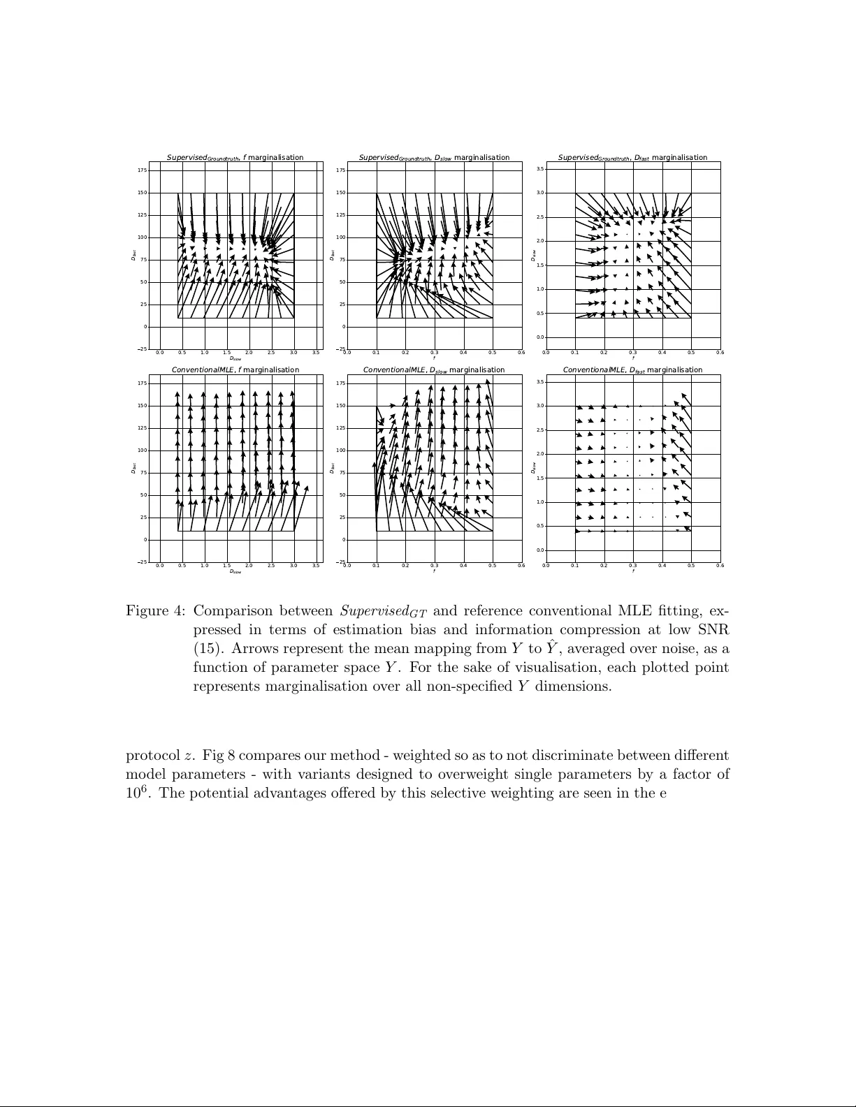
Journal of Machine Learning for Biomedical Imaging 2024:002 vol. 2, pp. 586–610 Submitted 06/2023 Published 02/2024 Choice of training lab el matters: ho w to b est use deep learning for quan titativ e MRI parameter estima tion Sean C. Epstein rmapcep@ucl.ac.uk Centre for Medical Image Computing, Univ ersit y College London, London, UK Timoth y J. P . Bra y t.bray@ucl.ac.uk Centre for Medical Imaging, Univ ersit y College London, London, UK Margaret Hall-Craggs m.hall-craggs@ucl.ac.uk Centre for Medical Imaging , Univ ersit y College London, London, UK Hui Zhang gary .zhang@ucl.ac.uk Centre for Medical Image Computing, Univ ersit y College London, London, UK Abstract Deep learning (DL) is gaining p opularity as a parameter estimation metho d for quantita- tiv e MRI. A range of comp eting implementations ha ve b een prop osed, relying on either sup ervised or self-supervised learning. Self-sup ervised approac hes, sometimes referred to as unsupervised, hav e b een lo osely based on auto-encoders, whereas sup ervised methods ha ve, to date, b een trained on groundtruth lab els. These tw o learning paradigms hav e b een shown to hav e distinct strengths. Notably , self-sup ervised approaches offer low er-bias parameter estimates than their sup ervised alternatives. This result is coun terintuitiv e – incorp orating prior kno wledge with sup ervised lab els should, in theory , lead to impro ved accuracy . In this w ork, we show that this apparent limitation of sup ervised approaches stems from the na ¨ ıv e c hoice of groundtruth training lab els. By using intentional ly-non- gr oundtruth tr aining lab els , pre-computed via indep endent maximum likelihoo d estima- tion, we show that the low-bias parameter estimation previously asso ciated with self- sup ervised methods can b e replicated – and improv ed on – within a sup ervised learning framew ork. This approach sets the stage for a single, unifying, deep learning parame- ter estimation framew ork, based on sup ervised learning, where trade-offs b etw een bias and v ariance are made by careful adjustment of training lab el. Our co de is av ailable at https://github.com/seancepstein/training_labels . Keyw ords: quan titative MRI, diffusion MRI, deep learning 1. In tro duction Magnetic resonance imaging (MRI) is widely regarded as the premier clinical imaging modal- it y , in large part due to the unparalleled range of contrast mec hanisms a v ailable to it. Con ven tional MRI exploits this contrast in a purely qualitative manner: images provide only r elative information, such that vo xel intensities are only meaningful in the con text of their neigh b ours. In contrast, quan titative MRI (qMRI) provides quan titative images, where vo xel intensities are directly , and meaningfully , related to underlying tissue prop- erties. Compared to con ven tional MRI, this approach promises increased repro ducibility , in terpretability , and tissue insigh t, at the cost of time-in tensive image acquisition and p ost- pro cessing (Cercignani et al., 2018). © 2024 Epstein et al.. License: CC-BY 4.0 https://doi.org/10.59275/j.melba.2024- geb5 Training labels f or qMRI p arameter estima tion One of the biggest time and resource b ottlenecks in p ost-pro cessing is parameter esti- mation, whereb y a signal mo del is fit to the intensit y v ariation across multiple MR images acquired at different exp erimental settings. Each vo xel requires its own indep endent mo del fit: solving for the signal m odel parameters that b est describ ed the single vo xel’s data. The computational cost of this curv e-fitting pro cess, whic h scales with b oth vo xel num b er and mo del complexit y , has b ecome a b ottleneck for mo dern qMRI exp eriments. Accelerating curv e fittings with deep learning (DL) was first proposed more than 30 y ears ago (Bishop and Roach, 1992), but has only recently gained p opularity within the qMRI comm unity (Golko v et al., 2016; Bertleff et al., 2017; Liu et al., 2020; Barbieri et al., 2020; P alombo et al., 2020). Just lik e traditional metho ds, DL relies on mo del fitting, but the mo del b eing fit is a fundamentally different one. Instead of fitting a qMRI signal mo del to a single v oxel of interest (i.e. curve fitting), DL metho ds fit (“train”) a de ep neur al network (DNN) mo del to an ensemble of training vo xels. This mo del maps a single vo xel’s signal to its corresp onding qMRI parameters; the unknowns in its fitting are netw ork weigh ts, rather than qMRI parameters. Once this DNN mo del has b een fit to (“trained on”) the training data, parameter estimation is reduced to simply applying it to new unseen data, one v oxel at a time. This approach offers tw o broad adv antages ov er traditional fitting: (1) computational cost is amortised: despite b eing more computationally exp ensiv e than one-v oxel signal model fitting, DL training only needs to be p erformed once, for any n umber of v oxels; once trained, netw orks provide near-instantaneous parameter estimates on new data, and (2) computational cost is front-loaded: model training can b e p erformed aw ay from the clinic, b efore patien t data is acquired. T o date, most DL qMRI fitting metho ds hav e b een implemented within a sup ervised learning framework (Golko v et al., 2016; Bertleff et al., 2017; Y o on et al., 2018; Liu et al., 2020; Palom b o et al., 2020; Aliotta et al., 2021; Y u et al., 2021; Gyori et al., 2022). This approac h trains DNNs to predict groundtruth qMRI mo del parameters from noisy qMRI signals. When compared to conv en tional fitting, this approach has b een found to pro duce high bias, lo w v ariance parameter estimates (Grussu et al., 2021; Gy ori et al., 2022). An alternativ e class of DL methods has also b een prop osed, sometimes referred to as un- sup ervised learning (Barbieri et al., 2020; Mpt et al., 2021), but more accurately describ ed as self-sup ervised (introduction). In this framework, training labels are not explicitly pro vided, but are instead extracted by the netw ork from its training input. This lab el generation is designed such that the net work learns to predict signal mo del parameters corresp onding to noise-free signals that most-closely appro ximate noisy inputs. This self-supervised approac h has been found to pro duce similar results to con v entional non-DL fitting, i.e. low er bias and higher v ariance than its groundtruth-lab elled sup ervised alternative (Barbieri et al., 2020; Grussu et al., 2021). F rom an information theoretic standp oint, the comparison b etw een sup ervised and self- sup ervised p erformance raises an obvious unanswered question. Ho w can it b e that su- p ervised metho ds, whic h provide strictly more information during training than their self- sup ervised coun terparts, pro duce more biased parameter estimates? In this work we answer this question by showing that this apparent limitation of sup er- vised approaches stems purely from the selection of groundtruth training lab els. By using intentional ly-non-gr oundtruth tr aining lab els , pre-computed via indep enden t maxim um lik e- liho o d estimation, we sho w that the low-bias parameter estimation previously asso ciated 587 Epstein et al. with self-sup ervised metho ds can b e replicated – and improv ed on – within a sup ervised learning framew ork. This approach sets the stage for a single, unifying, deep learning parameter estimation framew ork, based on sup ervised learning, where trade-offs b etw een bias and v ariance can b e made, on an application-sp ecific basis, b y careful adjustment of training lab el. The rest of the pap er is organized as follows: Section 2 describ es existing DL parameter estimation approaches, our prop osed metho d, and ho w they relate to each other; Section 3 describ es the ev aluation of our metho d and its comparison to the state of the art; Section 4 con tains our findings; and Section 5 summarizes the con tribution and discusses future w ork. 2. Theory Quan titative MRI extracts biomarkers y from MR data x , pro ducing quan titative spatial maps. W e here describ e existing vo xelwise approaches to this problem (conv entional fitting and DL alternativ es) as well as our prop osed nov el me thod. 2.1 Con ven tional iterative fitting This method, which relies on maxim um lik eliho o d estimation (MLE), extracts biomarkers b y p erforming a v oxelwise mo del fit every time new data is acquired. An appropriate signal mo del M is required, parameterised by n y parameters of interest; for each com bination of y , the probability of observing the acquired data x is kno wn as the lik eliho o d L of those parameters: L ( x, z | y , ϵ ) = n z Y i =1 P ( x i , z i | y , ϵ ) (1) for n z acquisitions from sampling scheme z and noise mo del ϵ . The mo del parameters ˆ y whic h maximise the lik eliho o d L are assumed to b est represent the tissue contained within the v oxel of interest: ˆ y = arg max y L ( x, z | y , ϵ ) (2) Under a Gaussian noise mo del, this likelihoo d maximization reduces to the commonly-used non-linear least squares (NLLS): ˆ y = arg min y n z X i =1 ∥ M ( z i | y ) − x i ∥ 2 (3) under the assumption of signal mo del M asso ciated with groundtruth biomarkers y g t , sam- pling sc heme z , and noise ϵ : x = M ( z | y g t ) + ϵ (4) Eac h of these optimisations has n y unkno wns, which are solved for indep endently across differen t vo xels; the computational cost scales linearly with the n umber of vo xels n v . 588 Training labels f or qMRI p arameter estima tion Dev elopments in qMRI acquisition and analysis hav e led to increased (i) image spatial resolution (i.e. greater n v ) and (ii) mo del complexit y (i.e. greater n y ), such that conv en- tional MLE fitting has b ecome increasingly computationally exp ensiv e. 2.2 Existing deep learning metho ds Deep learning approac hes address this by reframing n v indep enden t problems into a single global mo del fit: learning the function F that maps any x to its corresp onding y g t : y g t = F ( x ) (5) Deep neural netw orks aim to approximate this function by comp osing a large but finite n umber of building-blo c k functions, parametrised by n p net work parameters p (“weigh ts”): ˆ y = ˆ F ( x | ˆ p ) (6) In this context, mo del fitting (“training”), is p erformed o ver net work parameters p and in volv es maximising ˆ F ’s mean performance o ver a large set of training examples; the trained net w ork is defined b y the b est-fit parameters ˆ p . This fitting problem, whilst more computationally exp ensiv e to solve than an y individual vo xel ( n v = 1) MLE, is only tackled once; once ˆ F is learn t, it can b e applied at negligible cost to new, unseen, data. This promise of rapid, zero-cost parameter estimation has led to the dev elopment of t wo broad classes of DL-based parameter estimation metho ds. Sup ervise d GT metho ds approximate F by minimising the difference b etw een a large num- b er of noise-free training lab els (groundtruth parameter v alues) and corresp onding netw ork outputs (noise-free parameter estimates); training loss is calculated in the parameter space Y : Sup ervised GT training loss = n train X i =1 ∥ W · ( ˆ y i − y g t,i ) ∥ 2 (7) where n train is the n umber of training samples and W is a tunable weigh t matrix which accoun ts for magnitude differences in signal mo del parameters. W is generally a diagonal matrix, with each diagonal elemen t W ii corresp onding to the relative w eighting of qMRI parameter y i ; setting W as the iden tit y matrix equally w eights all parameters in the training loss. These metho ds pro duce higher bias, lo wer v ariance parameter estimation than con v en- tional MLE fitting (Grussu et al., 2021; Gyori et al., 2022) and, by adjusting W , can b e tailored to selectively b o ost estimation p erformance on a subset of the parameter space Y . In contrast, Self-sup ervise d metho ds compute training loss within the signal space X , b y minimising the difference b etw een netw ork inputs (noisy signals) and a filtered represen- tation of net work outputs (noise-free signal estimates): Self-sup ervised training loss = n train X i =1 ∥ M ( z | ˆ y i ) − x i ∥ 2 (8) These metho ds, which p erform similarly to conv en tional MLE fitting, pro duce low er bias, higher v ariance parameter estimation than Sup ervise d GT (Grussu et al., 2021; Barbieri et al., 589 Epstein et al. 2020). Unlike Sup ervise d GT , the relativ e loss weigh ting of different signal mo del parameters is dictated b y sampling scheme z . Under Gaussian noise conditions, single-vo xel Self-sup ervise d loss (i.e. minimising the sum of squared differences b etw een a noisy signal and its noise-free signal estimate) is indistinguishable from the corresp onding ob jectiv e function in conv en tional fitting. In contrast, under the Rician noise conditions encoun tered in MRI acquisition(Gudb jartsson and Patz, 1995), Self-sup ervise d training loss no longer matches conv en tional fitting. In- deed, the sum of squared errors b etw een noisy signals and noise-free estimates is not an accurate difference metric in the presence of Rician noise. T o summarise: existing sup ervised DL techniques are asso ciated by high estimation bias, lo w v ariance, and end-user flexibility; in contrast, self-sup ervised metho ds hav e lo wer bias, higher v ariance, but are limited by the fact their loss is calculated in the signal space X . 2.3 Prop osed deep learning metho d In light of this, we prop ose Sup ervise d MLE , a nov el parameter estimation metho d which com bines the adv an tages of Sup ervise d GT and Self-sup ervise d metho ds. This me thod is con trasted to existing techniques in Fig 1. This metho d mimics Self-sup ervise d ’s lo w-bias p erformance by learning a regularised form of conv en tional MLE, but do es so in the parameter space Y , within a sup ervised learning framew ork. This addresses the limitations of Self-sup ervise d : Rician noise mo d- elling is incorp orated, and parameter loss w eighting is not limited by sampling scheme z . Our metho d learns ˆ F b y training on noisy signals paired with conv entional MLE lab els. These lab els act as pro xies for the groundtruth parameters we wish to estimate: Sup ervised MLE training loss = n train X i =1 ∥ W · ( ˆ y i − y M LE ,i ) ∥ 2 (9) where y M LE ,i is the maxim um lik eliho o d estimate asso ciated with the i th training sam- ple. Our metho d offers one final adv an tage ov er Self-sup ervise d approac hes. In addition to the parameter estimation improv emen ts relating to noise mo del correction and parame- ter loss weigh ting, it naturally interfaces with Sup ervise d GT . In so doing, it presents the opp ortunit y to combine low-bias and lo w-v ariance metho ds in to a single, tunable hybrid approac h, by a simple weigh ted sum of eac h metho d’s loss function: Hybrid training loss = α · Sup ervised MLE loss + (1 − α ) · Sup ervised GT loss (10) 3. Exp erimen tal ev aluation Three classes of netw ork w ere inv estigated and compared: Sup ervise d GT , Self-sup ervise d , and Sup ervise d MLE , as describ ed in Fig 1. Additionally , to control for differences in loss 590 Training labels f or qMRI p arameter estima tion Supervised GT Supervised MLE !"#$"$%& '()&*+$', Self - super vised -$.%& ! " ! !"# " ! $%& /01 Labels:( groundtr uth) paramet ers Labels: ) MLE) estimat es No(labels -$.%& ! " ! !"# 2#3 . 4 . 45 ( 6 $ % % 2#3 . 4 . 45 ( 6 $ % % -$.%& " ! !"# 2#3 . 4 . 45 ( 6 $ % % $'()*+ $'()*+ $'()*+ $'() , * !"# + ! Figure 1: Comparison b et ween our prop osed metho d ( Sup ervise d MLE ) and existing sup er- vised and self-sup ervised approac hes. function weigh ting b etw een sup ervised and unsup ervised metho ds, Self-sup ervise d was con- v erted into sup ervised form b y training Sup ervise d MLE on Gaussian-mo del based MLE la- b els. All mo dels are summarised in T able 1. T able 1: Summary of ev aluated parameter estimation net works. Y denotes parameter space; X denotes signal space. Net w ork name Loss space Lab el Lab el noise mo del Sup ervise d GT Y Groundtruth N/A Self-sup ervise d X N/A N/A Sup ervise d MLE, Rician Y MLE Rician Sup ervise d MLE, Gaussian Y MLE Gaussian All net works w ere trained and tested on the same datasets; differences in performance can b e attributed solely to differences in loss function form ulation and training lab el selec- tion. 591 Epstein et al. 3.1 Signal mo del The in trav o xel incoherent motion (IVIM) mo del (Le Bihan et al., 1986) was inv estigated as an exemplar 4-parameter non-linear qMRI mo del which p oses a non-trivial mo del fitting problem and is w ell-represented in the DL qMRI literature (Bertleff et al., 2017; Barbieri et al., 2020; Mpt et al., 2021; Mastropietro et al., 2022; Rozo wski et al., 2022): S ( b | S 0 , f , D slow , D f ast ) = S 0 ( f e − b ( D f ast + D slow ) + (1 − f ) e − bD slow ) (11) where S corresp onds to the signal mo del M , b corresp onds to the sampling scheme z , and [ S 0 , f , D slow , D f ast ] corresp onds to the parameter-vector y . In physical terms, IVIM is a t wo-compartmen t diffusion mo del, wherein signal decay arises from b oth molecular self-diffusion (describ ed by D slow ) and p erfusion-induced ‘pseudo-diffusion’ (describ ed by D f ast ). In Equation 11, S 0 is an intensit y normalisation factor and f denotes the signal fraction corresp onding to the p erfusing compartmen t. 3.2 Net work arc hitecture Net work arc hitecture w as harmonised across all netw ork v ariants, and represents a common c hoice in the existing qMRI literature (Barbieri et al., 2020): 3 fully connected hidden lay ers, eac h with a n umber of nodes matc hing the num b er of signal samples z (i.e. b-v alues), and an output lay er with a num b er of no des matc hing the n umber of mo del parameters. Wider (150 no des per la yer) and deep er (10 hidden la yers) net works w ere in vestigated and found to ha v e equiv alen t p erformance, during b oth training and testing, at the cost of increased training time. All netw orks were implemen ted in Pytorch 1.9.0 with exp onen tial linear unit activ ation functions (Clev ert et al., 2015); ELU performance is similar to ReLU, but is more robust to p o or netw ork weigh t initialisation. 3.3 T raining data T raining datasets w ere generated at SNR = [15 , 30] to inv estigate parameter estimation p erformance at b oth high and low noise levels. At each SNR, 100,000 noise-free signals w ere generated from uniform IVIM parameter distributions ( S 0 ∈ [0 . 8 , 1 . 2], f ∈ [0 . 1 , 0 . 5], D slow ∈ [0 . 4 , 3 . 0]10 − 3 mm 2 /s , D f ast ∈ [10 , 150]10 − 3 mm 2 /s , representing realistic tissue v alues), sampling them with a real-w orld acquisition proto col (Zhao et al., 2015) ( b = [0 , 10 , 20 , 30 , 50 , 80 , 100 , 200 , 400 , 800] s/mm 2 ), and adding Rician noise. T raining data gen- erativ e parameters w ere dra wn from uniform, rather than in-vivo, parameter distributions to minimise bias in net work parameter estimation(Gyori et al., 2022). Data were split 80/20 b e- t ween training and v alidation. MLE lab els were calculated using a b ound-constrained non- linear fitting algorithm, implemented with scipy.optimize.minimize , using either Rician log- lik eliho o d (for Sup ervise d MLE, Rician ) or sum of squared errors (for Sup ervise d MLE, Gaussian ) as fitting ob jective function. This algorithm was initialised with groundtruth v alues (i.e. generativ e y ) to impro ve fitting robustness and av oid lo cal minima. T raining/v alidation samples asso ciated with ‘p o or’ MLE lab els (defined as lying on the b oundary of the b ound- constrained estimation space) were held out during training and ignored during v alidation. 592 Training labels f or qMRI p arameter estima tion 3.4 Net work training Net work training was p erformed using an Adam optimizer (learning rate = 0.001, b etas = (0.9, 0.999), weigh t decay=0) as follo ws: Sup ervise d GT (at SNR 30) was trained 16 times on the same data, each time initialising with differen t netw ork weigh ts, to improv e robustness to lo cal minima during training. F rom this set of trained net works, a single Sup ervise d GT net work was selected on the basis of v alidation loss. The trained weigh ts of this selected net work were subsequently used to initialise all other net works; in this wa y , an y differences in net work performance could b e solely attributed to differences in training lab el selection and training loss formulation. In the case of sup ervised loss form ulations, the in ter-parameter w eight v ector W w as chosen as the inv erse of each parameter’s mean v alue ov er the training set, to obtain equal loss w eighting across all four IVIM parameters. 3.5 T esting data Net works were tested on b oth synthetic and real qMRI data. The synthetic approach offers (i) known parameter groundtruths to assess estimation against, (ii) arbitrarily large datasets, and (iii) tunable data distributions, but is based on p ossibly simplified qMRI signals. This approac h w as used to assess parameter estimation p erformance in a c on trolled, rigorous manner; real data w as subsequently used to v alidate the trends observ ed in silico. Syn thetic data was generated with sampling, parameter distributions, and noise levels matc hing those used in netw ork training. The IVIM parameter space in which the net works w ere trained was uniformly sub-divided 10 times in each dimension, to analyse estimation p erformance as a function of parameter v alue. A t each p oint in the parameter space, 500 corresp onding noisy signals were generated and used to test net work p erformance, accoun ting for v ariation under noise rep etition. Real data was acquired from the p elvis of a health y volun teer, who gav e informed con- sen t, on a wide-b ore 3.0T clinical system (Ingenia, Philips, Amsterdam, Netherlands), 5 slices, 224 x 224 matrix, v oxel size = 1.56 x 1.56 x 7mm, TE = 76ms, TR = 516ms, scan time = 44s p er 10 b-v alues listed in subsection 3.3. F or the purp oses of assessing parameter estimation methods, we obtained gold standard v oxelwise IVIM parameter estimates from a sup ersampled dataset (16-fold rep etition of the ab ov e acquisition, within a single scanning session, generating 160 b-v alues, total scan time = 11m44s). Conv entional MLE w as p er- formed on this supersampled data to pro duce b est-guess “groundtruth” parameters. During testing, the sup ersampled dataset was split into 16 distinct 10 b-v alue acquisitions, eac h corresp onding to a single realistic clinical acquisition. All images w ere visually confirmed to b e free from motion artefacts. The mismatch in parameter distributions b etw een this in-viv o data (highly non-uniform) and the previously-describ ed syn thetic data (uniform by construction) limited the scop e for v alidating our in-silico results. T o address this, a fi- nal syn thetic testing dataset was generated from the in-viv o MLE-derived “groundtruth” parameters, and w as used for direct comparison b etw een real and sim ulated data. 3.6 Ev aluation metrics P arameter estimation p erformance was ev aluated using 3 key metrics: (i) mean bias with resp ect to groundtruth, (ii) mean standard deviation under noise rep etition, and (iii) ro ot 593 Epstein et al. mean squared error (RMSE) with resp ect to groundtruth. RMSE is the most commonly used metric to ev aluate estimation p erformance (Barbieri et al., 2020; Bertleff et al., 2017), but is limited in its abilit y to disentangle accuracy and precision; to this end, mean bias and standard deviation w ere used as more sp ecific measures of netw ork p erformance. It is imp ortant to note that al l metho ds were assessed with resp ect to groundtruth qMRI parameters, even those tr aine d on MLE lab els . F or these metho ds, the training and v alidation loss (MLE-based) differed from the rep orted testing loss (groundtruth-based). 4. Results & discussion This section summarises our main findings and discusses the adv an tages offered by the parameter estimation metho d w e prop ose. 4.1 Comparison of parameter estimation metho ds The relativ e p erformance of all previously-discussed parameter estimation metho ds is sum- marised in Figures 2 and 3. These figures show the bias, v ariance (represented b y its square ro ot: standard deviation), and RMSE of parameter estimates with respect to groundtruth v alues, rep orted for eac h mo del parameter as a function of its v alue ov er the synthetic test dataset; each plotted p oint represen ts an av erage ov er 500 noise instan tiations and a marginalisation o ver all non-visualised parameters. Marginalisation was required for visu- alisation of a 4-dimensional parameter space, but was confirmed to b e representativ e of the en tire, non-marginalised space, as discussed in § 4.5. In keeping with previously reported results, we sho w a bias/v ariance trade-off b etw een differen t parameter estimation metho ds. Con ven tional MLE fitting is provided as a reference (plotted in black). Approaches whic h, on a theoretical lev el, appro ximate con ven tional MLE ( Self-sup ervise d and Sup ervise d MLE , plotted in red), are generally asso ciated with low bias, high v ariance, and high RMSE, whereas groundtruth-lab elled sup ervised metho ds (plotted in blue) exhibit lo wer v ariance and RMSE at the cost of increased bias. Increases in bias, if consisten t across parameter space Y , do not necessarily reduce sen- sitivit y to differences in underlying tissue prop erties. Ho wev er, we sho w that S uper v ised GT is asso ciated with bias that varies signific antly as a function of groundtruth parameter v al- ues. This results in a reduction in information con ten t, visualised as the gr adient of the bias plots (top row) in Fig 2. The more negative the gradient, the more parameter estimates are concen trated in the centre of the parameter estimation space ˆ X , and the low er the ability of the method to distinguish differences in tissue prop erties. This information loss can be seen in Fig 4, whic h compares S uperv ised GT to conv entional MLE fitting, and sho ws the compression in ˆ X ov er the groundtruth parameter-space X . 4.2 V alidation against clinical data The ab ov e trends, found in sim ulation, were also observed in real-w orld data. Fig 5 sho ws the bias, v ariance, and RMSE of parameter estimates with resp ect to “groundtruth” v alues (obtained from the sup ersampled dataset describ ed in § 3.5). The x axes of these plots cor- resp ond to these reference v alues. T o aid visualisation, 10 uniform bins were constructed along each parameter dimension, in to whic h clinical vo xels w ere assigned based on their 594 Training labels f or qMRI p arameter estima tion 0.10 0.15 0.20 0.25 0.30 0.35 0.40 0.45 0.50 0.06 0.04 0.02 0.00 0.02 0.04 0.06 Bias f C o n v e n t i o n a l M L E S u p e r v i s e d M L E , R i c i a n S u p e r v i s e d M L E , G a u s s i a n S e l f s u p e r v i s e d S u p e r v i s e d G r o u n d t r u t h 0.5 1.0 1.5 2.0 2.5 3.0 0.4 0.3 0.2 0.1 0.0 0.1 0.2 0.3 0.4 Bias D s l o w 20 40 60 80 100 120 140 60 40 20 0 20 40 60 Bias D f a s t 0.10 0.15 0.20 0.25 0.30 0.35 0.40 0.45 0.50 0.00 0.02 0.04 0.06 0.08 0.10 0.12 0.14 Standar d deviation 0.5 1.0 1.5 2.0 2.5 3.0 0.0 0.1 0.2 0.3 0.4 0.5 0.6 0.7 0.8 Standar d deviation 20 40 60 80 100 120 140 0 20 40 60 80 100 120 Standar d deviation 0.10 0.15 0.20 0.25 0.30 0.35 0.40 0.45 0.50 P arameter value 0.00 0.02 0.04 0.06 0.08 0.10 0.12 0.14 RMSE 0.5 1.0 1.5 2.0 2.5 3.0 P arameter value 0.0 0.1 0.2 0.3 0.4 0.5 0.6 0.7 0.8 RMSE 20 40 60 80 100 120 140 P arameter value 0 20 40 60 80 100 120 RMSE Figure 2: P arameter estimation p erformance at low SNR (15) as a function of groundtruth parameter Y . P erformance summarised by bias & RMSE with resp ect to groundtruth and standard deviation with resp ect to noise rep etition. Con v en- tional MLE fitting is provided as a non-DNN reference standard. F or the sak e of visualisation, each plotted p oin t represen ts marginalisation o ver all non-sp ecified Y dimensions. “groundtruth” parameter v alues. Fig 5 plots the mean bias, standard deviation, and RMSE asso ciated with each bin as a function of the bin’s cent ral v alue, together with the distri- bution of v oxels across the 10 bins. By calculating the v ariance of the 16 b = 0 images, the SNR of this clinical dataset was found to b e ∼ 15; Fig 2 is therefore the relev ant p oint of comparison. It can b e readily seen that the trends observ ed in simulated data, describ ed in § 4.1, are replicated for f < 0 . 40, D slow < 1 . 5, and the en tire range of D f ast , namely the regions of parameter-space whic h are well-represen ted in the real-world data. Fig 6 confirms that div ergence outside of these ranges is due to under-representation in the in vivo test data; the apparent div ergences can b e replicated in-silico b y matching real-world parameter distributions. Fig 7 contains exemplar parameter maps from the clinical test data, and shows the real-w orld implications of the trends summarised in Figures 2 and 5: S uper v ised GT ’s low- 595 Epstein et al. 0.10 0.15 0.20 0.25 0.30 0.35 0.40 0.45 0.50 0.04 0.03 0.02 0.01 0.00 0.01 0.02 0.03 0.04 Bias f C o n v e n t i o n a l M L E S u p e r v i s e d M L E , R i c i a n S u p e r v i s e d M L E , G a u s s i a n S e l f s u p e r v i s e d S u p e r v i s e d G r o u n d t r u t h 0.5 1.0 1.5 2.0 2.5 3.0 0.2 0.1 0.0 0.1 0.2 Bias D s l o w 20 40 60 80 100 120 140 30 20 10 0 10 20 30 Bias D f a s t 0.10 0.15 0.20 0.25 0.30 0.35 0.40 0.45 0.50 0.00 0.01 0.02 0.03 0.04 0.05 0.06 0.07 0.08 Standar d deviation 0.5 1.0 1.5 2.0 2.5 3.0 0.0 0.1 0.2 0.3 0.4 Standar d deviation 20 40 60 80 100 120 140 0 10 20 30 40 50 60 70 Standar d deviation 0.10 0.15 0.20 0.25 0.30 0.35 0.40 0.45 0.50 P arameter value 0.00 0.01 0.02 0.03 0.04 0.05 0.06 0.07 0.08 RMSE 0.5 1.0 1.5 2.0 2.5 3.0 P arameter value 0.0 0.1 0.2 0.3 0.4 RMSE 20 40 60 80 100 120 140 P arameter value 0 10 20 30 40 50 60 70 RMSE Figure 3: P arameter estimation p erformance, visualised as in Figure 2, but for high SNR (30) data. v ariance, low-RMSE parameter estimation results in artificially smo oth IVIM maps biased to wards mean parameter v alues. 4.3 Adv antages offered by our metho d Our prop osed metho d o ccupies the low-bias side of the bias-v ariance trade-off discussed in § 3.5, and offers four broad adv antages ov er the comp eting metho d in this space ( Self- sup ervise d ): (i) flexibility in c ho osing inter-parameter loss w eigh ting W , (ii) incorp oration of non-Gaussian (e.g. Rician) noise mo dels, (iii) compatibility with complex, non-differentiable signal mo dels M , and (iv) ability to interface with low-v ariance metho ds, to pro duce a h ybrid approac h tunable to the needs of the task at hand. These adv antages are analysed in turn. 4.3.1 Choice of inter-p arameter loss weighting W By computing loss in parameter-space Y , our metho d has total flexibilit y in adjusting the relativ e contribution of different y in the training loss function. In contrast, since Self- sup ervise d calculates training loss in X , the relativ e weigh ting dep ends on the acquisition 596 Training labels f or qMRI p arameter estima tion 0.0 0.5 1.0 1.5 2.0 2.5 3.0 3.5 D s l o w 25 0 25 50 75 100 125 150 175 D f a s t S u p e r v i s e d G r o u n d t r u t h , f m a r g i n a l i s a t i o n 0.0 0.1 0.2 0.3 0.4 0.5 0.6 f 25 0 25 50 75 100 125 150 175 D f a s t S u p e r v i s e d G r o u n d t r u t h , D s l o w m a r g i n a l i s a t i o n 0.0 0.1 0.2 0.3 0.4 0.5 0.6 f 0.0 0.5 1.0 1.5 2.0 2.5 3.0 3.5 D s l o w S u p e r v i s e d G r o u n d t r u t h , D f a s t m a r g i n a l i s a t i o n 0.0 0.5 1.0 1.5 2.0 2.5 3.0 3.5 D s l o w 25 0 25 50 75 100 125 150 175 D f a s t C o n v e n t i o n a l M L E , f m a r g i n a l i s a t i o n 0.0 0.1 0.2 0.3 0.4 0.5 0.6 f 25 0 25 50 75 100 125 150 175 D f a s t C o n v e n t i o n a l M L E , D s l o w m a r g i n a l i s a t i o n 0.0 0.1 0.2 0.3 0.4 0.5 0.6 f 0.0 0.5 1.0 1.5 2.0 2.5 3.0 3.5 D s l o w C o n v e n t i o n a l M L E , D f a s t m a r g i n a l i s a t i o n Figure 4: Comparison b etw een Sup ervise d GT and reference conv en tional MLE fitting, ex- pressed in terms of estimation bias and information compression at lo w SNR (15). Arrows represen t the mean mapping from Y to ˆ Y , av eraged ov er noise, as a function of parameter space Y . F or the sake of visualisation, each plotted p oin t represen ts marginalisation ov er all non-sp ecified Y dimensions. proto col z . Fig 8 compares our metho d - weigh ted so as to not discriminate betw een different mo del parameters - with v arian ts designed to o verw eight single parameters b y a factor of 10 6 . The p otential adv antages offered by this se lectiv e weigh ting are seen in the estimation D f ast , where this approach leads to a small increase in b oth precision and accuracy . This parameter-sp ecific w eighting is not accessible within a Self-sup ervise d framework. In ligh t of the differences arising from inter-parameter loss weigh ting, for subsequen t analysis we use Sup ervise d MLE, Gaussian as a proxy for Self-sup ervise d ; b oth metho ds enco de the same regularised MLE fitting, but differ in their in ter-parameter weigh ting. 4.3.2 Incorpora tion of Rician noise modelling By pre-computing MLE lab els using conv entional parameter estimation metho ds, we are able to incorp orate accurate Rician noise mo delling. Comparison b etw een Sup ervise d MLE, Rician and Sup ervise d MLE, Gaussian sho ws the effect of the c hoice of noise mo del; these differences 597 Epstein et al. 0.10 0.15 0.20 0.25 0.30 0.35 0.40 0.45 0.50 0.08 0.06 0.04 0.02 0.00 0.02 0.04 0.06 0.08 Bias f 0.5 1.0 1.5 2.0 2.5 3.0 0.4 0.3 0.2 0.1 0.0 0.1 0.2 0.3 0.4 Bias D s l o w C o n v e n t i o n a l M L E S u p e r v i s e d M L E , R i c i a n S e l f s u p e r v i s e d S u p e r v i s e d M L E , G a u s s i a n S u p e r v i s e d G r o u n d t r u t h 20 40 60 80 100 120 140 60 40 20 0 20 40 60 Bias D f a s t 0.10 0.15 0.20 0.25 0.30 0.35 0.40 0.45 0.50 0.00 0.02 0.04 0.06 0.08 0.10 0.12 0.14 0.16 Standar d deviation 0.5 1.0 1.5 2.0 2.5 3.0 0.0 0.1 0.2 0.3 0.4 0.5 0.6 0.7 0.8 Standar d deviation 20 40 60 80 100 120 140 0 20 40 60 80 100 120 Standar d deviation 0.10 0.15 0.20 0.25 0.30 0.35 0.40 0.45 0.50 P arameter value 0.00 0.02 0.04 0.06 0.08 0.10 0.12 0.14 0.16 RMSE 0.5 1.0 1.5 2.0 2.5 3.0 P arameter value 0.0 0.1 0.2 0.3 0.4 0.5 0.6 0.7 0.8 RMSE 20 40 60 80 100 120 140 P arameter value 0 20 40 60 80 100 120 RMSE 0.10 0.15 0.20 0.25 0.30 0.35 0.40 0.45 0.50 0 500 1000 1500 2000 2500 3000 Bin count 0.5 1.0 1.5 2.0 2.5 3.0 0 500 1000 1500 2000 2500 Bin count 20 40 60 80 100 120 140 0 500 1000 1500 2000 2500 3000 Bin count Figure 5: In viv o parameter estimation p erformance of netw orks trained on low SNR (15) syn thetic data, as a function of supersampling-derived reference parameter v al- ues. The first three ro ws summarise p erformance by sho wing bias & RMSE with resp ect to reference v alue and standard deviation with resp ect to noise rep eti- tion, marginalised ov er all non-sp ecified Y dimensions. The b ottom row shows the distribution of reference parameter v alues across the parameter range b eing visualised. are most pronounced at lo w SNR (Fig 2) and high D slow , when the Gaussian appro ximation of Rician noise is known to break down. In this regime, our metho d gives less biased, more informativ e D slow estimates, replicating con ven tional MLE p erformance at a fraction of the 598 Training labels f or qMRI p arameter estima tion 0.10 0.15 0.20 0.25 0.30 0.35 0.40 0.45 0.50 0.08 0.06 0.04 0.02 0.00 0.02 0.04 0.06 0.08 Bias f 0.5 1.0 1.5 2.0 2.5 3.0 0.4 0.3 0.2 0.1 0.0 0.1 0.2 0.3 0.4 Bias D s l o w C o n v e n t i o n a l M L E S u p e r v i s e d M L E , R i c i a n S e l f s u p e r v i s e d S u p e r v i s e d M L E , G a u s s i a n S u p e r v i s e d G r o u n d t r u t h 20 40 60 80 100 120 140 60 40 20 0 20 40 60 Bias D f a s t 0.10 0.15 0.20 0.25 0.30 0.35 0.40 0.45 0.50 0.00 0.02 0.04 0.06 0.08 0.10 0.12 0.14 0.16 Standar d deviation 0.5 1.0 1.5 2.0 2.5 3.0 0.0 0.1 0.2 0.3 0.4 0.5 0.6 0.7 0.8 Standar d deviation 20 40 60 80 100 120 140 0 20 40 60 80 100 120 Standar d deviation 0.10 0.15 0.20 0.25 0.30 0.35 0.40 0.45 0.50 P arameter value 0.00 0.02 0.04 0.06 0.08 0.10 0.12 0.14 0.16 RMSE 0.5 1.0 1.5 2.0 2.5 3.0 P arameter value 0.0 0.1 0.2 0.3 0.4 0.5 0.6 0.7 0.8 RMSE 20 40 60 80 100 120 140 P arameter value 0 20 40 60 80 100 120 RMSE 0.10 0.15 0.20 0.25 0.30 0.35 0.40 0.45 0.50 0 500 1000 1500 2000 2500 3000 Bin count 0.5 1.0 1.5 2.0 2.5 3.0 0 500 1000 1500 2000 2500 Bin count 20 40 60 80 100 120 140 0 500 1000 1500 2000 2500 3000 Bin count Figure 6: P arameter estimation p erformance of net works trained on low SNR (15) syn thetic data, tested on a synthetic dataset matc hing the distribution of in vivo reference parameter v alues. The first three rows summarise p erformance by showing bias & RMSE with resp ect to groundtruth v alue and standard deviation with resp ect to noise rep etition, marginalised o ver all non-sp ecified Y dimensions. The b ottom ro w shows the distribution of groundtruth parameter v alues across the parameter range, whic h matches the in vivo dataset by construction. computational cost. At high D slow , our metho d has a flatter, more information-ric h, D slow bias curve than all other DL methods. This information loss is further visualised in Fig 9, whic h shows the compression in D slow estimates ˆ X ov er the groundtruth parameter-space 599 Epstein et al. f Super -sampled gr oundtruth f Conventional MLE f Supervised (MLE) f Self -supervised f Supervised (gr oundtruth) D s l o w D s l o w D s l o w D s l o w D s l o w D f a s t D f a s t D f a s t D f a s t D f a s t 0.0 0.1 0.2 0.3 0.4 0.5 0.0 0.5 1.0 1.5 2.0 2.5 3.0 3.5 4.0 0 50 100 150 200 250 300 0.0 0.1 0.2 0.3 0.4 0.5 0.0 0.5 1.0 1.5 2.0 2.5 3.0 3.5 4.0 0 50 100 150 200 250 300 0.0 0.1 0.2 0.3 0.4 0.5 0.0 0.5 1.0 1.5 2.0 2.5 3.0 3.5 4.0 0 50 100 150 200 250 300 0.0 0.1 0.2 0.3 0.4 0.5 0.0 0.5 1.0 1.5 2.0 2.5 3.0 3.5 4.0 0 50 100 150 200 250 300 0.0 0.1 0.2 0.3 0.4 0.5 0.0 0.5 1.0 1.5 2.0 2.5 3.0 3.5 4.0 0 50 100 150 200 250 300 Figure 7: P arameter estimation p erformance of netw orks on real-world test data, visualised as spatial maps. Groundtruth maps are taken as the maxim um likelihoo d param- eter estimates asso ciated with the complete 160 b-v alue dataset, whereas netw ork predictions are obtained from a single 10 b-v alue subsample. X . As exp ected, this compression is most apparent at high v alues of D slow , when the signal is more lik ely to approach the Rician noise flo or. 4.3.3 Comp a tibility with complex signal models An additional adv an tage of computing training loss in parameter-space Y is that DNN net works are signal mo del agnostic: net w ork training do es not require explicit calculation of M . This approac h is adv an tageous when working with complex signal mo dels, as made clear b y comparison with Self-sup ervise d metho ds. In contrast with our proposed approach, Self-sup ervise d metho ds em b ed M b etw een netw ork output and training loss (see Fig 1); this p oses t wo practical limitations. The first relates to efficient implementation of mini-batc h loss, which requires a v ec- torised representation (and calculation) of predicted signals. This may p ose a non-trivial c hallenge in the case of complex signal mo dels. The second limitation relates to ho w train- ing loss is minimised: netw ork parameters p are updated by computing partial deriv atives of the training loss. This pro cess requires the loss to be expressed in a differentiable form; em b edding M in the loss form ulation limits Self-sup ervise d metho ds to signal mo dels that can b e expressed in an explicitly differen tiable form. 600 Training labels f or qMRI p arameter estima tion 0.10 0.15 0.20 0.25 0.30 0.35 0.40 0.45 0.50 0.04 0.02 0.00 0.02 0.04 Bias f S u p e r v i s e d M L E , R i c i a n W e i g h t e d S u p e r v i s e d M L E , R i c i a n 0.5 1.0 1.5 2.0 2.5 3.0 0.3 0.2 0.1 0.0 0.1 0.2 0.3 Bias D s l o w 20 40 60 80 100 120 140 40 20 0 20 40 Bias D f a s t 0.10 0.15 0.20 0.25 0.30 0.35 0.40 0.45 0.50 0.00 0.02 0.04 0.06 0.08 0.10 Standar d deviation 0.5 1.0 1.5 2.0 2.5 3.0 0.0 0.1 0.2 0.3 0.4 0.5 0.6 0.7 Standar d deviation 20 40 60 80 100 120 140 0 20 40 60 80 100 Standar d deviation 0.10 0.15 0.20 0.25 0.30 0.35 0.40 0.45 0.50 P arameter value 0.00 0.02 0.04 0.06 0.08 0.10 RMSE 0.5 1.0 1.5 2.0 2.5 3.0 P arameter value 0.0 0.1 0.2 0.3 0.4 0.5 0.6 0.7 RMSE 20 40 60 80 100 120 140 P arameter value 0 20 40 60 80 100 RMSE Figure 8: Comparison b etw een Sup ervise d MLE, Rician , as describ ed ab o ve, and v ariants whic h differ in their in ter-parameter loss w eighting W , at lo w SNR (15). Each column compares Sup ervise d MLE, Rician to a different net work v ariant, uniquely trained to ov erw eight the single relev ant signal mo del parameter. F or the sake of visualisation, each plotted p oin t represen ts marginalisation o ver all non-sp ecified Y dimensions. Our metho d sidesteps b oth limitations by not requiring explicit calculation of M during training, and is therefore compatible with a wider range of complex qMRI signal mo dels. 4.3.4 Tunable netw ork appr oa ch As discussed ab ov e, w e show a clear bias/v ariance trade-off b etw een differen t parameter estimation metho ds. The optimal c hoice of metho d depends on the task at hand (Epstein et al., 2021), and may not lie at either extreme of this trade-off. Therefore, it w ould b e adv antageous to be able to combine lo w-bias and lo w-v ariance metho ds in to a single, hybrid approac h, with p erformance tunable by the relative contribution of each constituen t metho d. Our prop osed metho d, whic h interfaces naturally with S uper v ised GT , offers exactly that. An example of this approach is sho wn in Fig 10: training loss has b een weigh ted equally 601 Epstein et al. 0.0 0.1 0.2 0.3 0.4 0.5 0.6 f 0.0 0.5 1.0 1.5 2.0 2.5 3.0 3.5 D s l o w S u p e r v i s e d M L E , G a u s s i a n , D f a s t m a r g i n a l i s a t i o n 0.0 0.1 0.2 0.3 0.4 0.5 0.6 f 0.0 0.5 1.0 1.5 2.0 2.5 3.0 3.5 D s l o w S u p e r v i s e d M L E , R i c i a n , D f a s t m a r g i n a l i s a t i o n Figure 9: Comparison of the information conten t captured by Sup ervise d MLE metho ds , as a function of the noise mo del used in computing MLE lab els, at lo w SNR (15). Arro ws represen t the mean mapping from Y to ˆ Y , av eraged ov er noise, as a function of parameter space Y . F or the sake of visualisation, each plotted p oin t represen ts marginalisation ov er all non-sp ecified Y dimensions. ( α = 0 . 5) b etw een groundtruth and MLE lab els, and, as exp ected, the resulting net work p erformance lies in the middle ground b et ween these tw o extremes. 4.3.5 Comp arison with conventional fitting Comparison b etw een our prop osed metho d ( Sup ervise d MLE, Rician ) and conv en tional fitting ( MLE, R ician ) highligh ts additional adv antages offered b y our approac h. Firstly , Figs 2 and 3 demonstrate qualitativ ely similar p erformance b et ween these metho ds across the entire parameter space. The fact that our metho d, which offers near-instantaneous parameter estimation, produces similar parameter estimates to w ell-understo o d con ven tional MLE metho ds justifies its adoption in and of itself. Ho wev er, our metho d not only mimics but indeed in many cases outp erforms (low er bias, v ariance, and RMSE) the very same metho d used to compute those lab els. This result not only motiv ates its use, but also confirms that DL metho ds are able to exploit information shared b et ween training samples b eyond what w ould b e p ossible by considering each sample in isolation. 602 Training labels f or qMRI p arameter estima tion 0.10 0.15 0.20 0.25 0.30 0.35 0.40 0.45 0.50 0.06 0.04 0.02 0.00 0.02 0.04 0.06 Bias f S u p e r v i s e d M L E , R i c i a n S u p e r v i s e d G T H y b r i d 0.5 1.0 1.5 2.0 2.5 3.0 0.4 0.3 0.2 0.1 0.0 0.1 0.2 0.3 0.4 Bias D s l o w 20 40 60 80 100 120 140 40 20 0 20 40 Bias D f a s t 0.10 0.15 0.20 0.25 0.30 0.35 0.40 0.45 0.50 0.00 0.02 0.04 0.06 0.08 0.10 0.12 0.14 Standar d deviation 0.5 1.0 1.5 2.0 2.5 3.0 0.0 0.1 0.2 0.3 0.4 0.5 0.6 0.7 0.8 Standar d deviation 20 40 60 80 100 120 140 0 20 40 60 80 100 Standar d deviation 0.10 0.15 0.20 0.25 0.30 0.35 0.40 0.45 0.50 P arameter value 0.00 0.02 0.04 0.06 0.08 0.10 0.12 0.14 RMSE 0.5 1.0 1.5 2.0 2.5 3.0 P arameter value 0.0 0.1 0.2 0.3 0.4 0.5 0.6 0.7 0.8 RMSE 20 40 60 80 100 120 140 P arameter value 0 20 40 60 80 100 RMSE Figure 10: Pro of of concept of a hybrid parameter estimation metho d, formed by training a sup ervised netw ork with an equally-weigh ted sum of Sup ervise d MLE, Rician and Sup ervise d GT loss functions ( α = 0 . 5), at low SNR (15). F or the sake of visu- alisation, eac h plotted p oint represents marginalisation o ver all non-sp ecified Y dimensions. 4.4 A note on RMSE W e note that RMSE is a p o or summary measure of netw ork p erformance. RMSE is hea vily sk ewed b y outliers, and thus fav ours metho ds which giv e parameter estimates consistently close to mean parameter v alues. Such estimates, as in the case of D f ast , may contain v ery little information (Fig 4) despite b eing asso ciated with low RMSE. Accordingly , we strongly recommend that RMSE b e discontin ued as a single summary metric for parameter estimation p erformance: it must alw ays b e accompanied by bias, v ariance, and ideally an analysis of information con tent. RMSE’s limitations as a p erformance metric during testing may also call in to question its suitabilit y as a loss metric during tr aining . This work, muc h lik e the rest of the DL qMRI literature, employs a training loss (MSE, describ ed in Sections 2.2 and 2.3) which is monotonically related to RMSE. Whilst outside the scop e of this work, implemen ting 603 Epstein et al. a non-RMSE-derived training loss (suc h as mean absolute error) may b e w orth of future in vestigation. 4.5 Justification of parameter marginalisation The ab ov e analysis has b een largely based on Figs 2 and 3, which show parameter estimation p erformance marginalised ov er 3 dimensions of X . This choice, made to aid visualisation, w as v alidated against higher dimensional represen tations of the same data. Fig 11 compares Sup ervise d MLE, Rician and Sup ervise d Gr oundtruth p erformance across the en tire qMRI parameter space. It can b e seen that trends observed in Fig 2 are replicated here; we draw attention to t w o such examples. Firstly , Fig 2 suggests Sup ervise d Gr oundtruth pro duces lo wer f standard deviation than Sup ervise d MLE, Rician ; Fig 11 confirms this to b e the case across all test data. In contrast, Fig 2 suggests that Sup ervise d Gr oundtruth pro duces higher D slow bias at lo w D slow and lo w er bias at high D slow ; Fig 11 confirms a spread of bias differences across the test data: some fav ouring one metho d, and others the other. This effect is explored in Fig 12, which compares D slow estimation p erformance as a function of f and D f ast at t wo sp ecific (non-marginalised) groundtruth D slow v alues (0 . 69 , 2 . 71). As exp ected from the marginalised representation in Fig 2, at lo w D slow Sup ervise d Gr oundtruth pro duces higher bias acr oss the entir e f - D f ast p ar ameter sp ac e , whereas at high D slow the opp osite is true. Despite this, it is important to note the limitations of marginalisation. Fig 12 also sho ws that the relative performance of Sup ervise d MLE, Rician and Sup ervise d Gr oundtruth v aries across al l p ar ameter-sp ac e dimensions . Consider D slow = 0 . 69, where 2 shows similar marginalised RMSE for these methods. In fact, by visualising this difference as a function of f and D f ast , w e reveal t wo distinct regions: high f /low D f ast (where Sup ervise d MLE, Rician pro duces low er RMSE), and elsewhere (where it pro duces higher RMSE). This highlights (i) the p otential pitfalls of pro ducing summary results by marginalising across entire parameter spaces and (ii) the need to c ho ose parameter-estimation methods appropriate for the specific parameter com binations relev an t to the tissues b eing inv estigated (Epstein et al., 2021). 4.6 Non-v oxelwise approac hes This work has focused on vo xelwise DL parameter estimation metho ds: netw orks whic h map one signal curv e to its corresp onding parameter estimate. There are, how ever, alternativ es: con volutional neural netw ork metho ds whic h map spatially related clusters (“patches”) of qMRI signals to corresp onding clusters of parameter estimates (F ang et al., 2017; Ulas et al., 2019; Li et al., 2022). Our MLE training label approac h could b e incorporated in to suc h metho ds, and we lea ve it to future w ork to in vestigate the effect this would ha ve on parameter estimation p erformance. 5. Conclusions In this work we draw inspiration from state-of-the-art sup ervised and self-sup ervised qMRI parameter estimation metho ds to prop ose a no vel DNN approach which combines their resp ectiv e strengths. In keeping with previous work, w e demonstrate the presence of a 604 Training labels f or qMRI p arameter estima tion 0.20 0.15 0.10 0.05 0.00 0.05 B i a s : S u p e r v i s e d G r o u n d t r u t h 0.20 0.15 0.10 0.05 0.00 0.05 B i a s : S u p e r v i s e d M L E , R i c i a n f 0.4 0.2 0.0 0.2 0.4 0.6 0.8 B i a s : S u p e r v i s e d G r o u n d t r u t h 0.4 0.2 0.0 0.2 0.4 0.6 0.8 B i a s : S u p e r v i s e d M L E , R i c i a n D s l o w 60 40 20 0 20 40 60 B i a s : S u p e r v i s e d G r o u n d t r u t h 60 40 20 0 20 40 60 B i a s : S u p e r v i s e d M L E , R i c i a n D f a s t 0.02 0.04 0.06 0.08 0.10 0.12 0.14 S t a n d a r d d e v i a t i o n : S u p e r v i s e d G r o u n d t r u t h 0.02 0.04 0.06 0.08 0.10 0.12 0.14 S t a n d a r d d e v i a t i o n : S u p e r v i s e d M L E , R i c i a n 0.1 0.2 0.3 0.4 0.5 0.6 0.7 S t a n d a r d d e v i a t i o n : S u p e r v i s e d G r o u n d t r u t h 0.1 0.2 0.3 0.4 0.5 0.6 0.7 S t a n d a r d d e v i a t i o n : S u p e r v i s e d M L E , R i c i a n 20 40 60 80 100 S t a n d a r d d e v i a t i o n : S u p e r v i s e d G r o u n d t r u t h 20 40 60 80 100 S t a n d a r d d e v i a t i o n : S u p e r v i s e d M L E , R i c i a n 0.05 0.10 0.15 0.20 R M S E : S u p e r v i s e d G r o u n d t r u t h 0.025 0.050 0.075 0.100 0.125 0.150 0.175 0.200 0.225 R M S E : S u p e r v i s e d M L E , R i c i a n 0.2 0.4 0.6 0.8 1.0 R M S E : S u p e r v i s e d G r o u n d t r u t h 0.2 0.4 0.6 0.8 1.0 R M S E : S u p e r v i s e d M L E , R i c i a n 20 40 60 80 100 R M S E : S u p e r v i s e d G r o u n d t r u t h 20 40 60 80 100 R M S E : S u p e r v i s e d M L E , R i c i a n Figure 11: Non-marginalised comparison of parameter estimation p erformance b etw een Sup ervise d MLE, Rician and Sup ervise d Gr oundtruth at low SNR (15). Colour inten- sit y represents density of distribution across all X and all noise rep etitions. bias/v ariance trade-off b etw een existing metho ds; sup ervised training pro duces lo w v ariance under noise, whereas self-sup ervised leads to lo w bias with resp ect to groundtruth. The increased bias of supervised DNNs is coun ter-intuitiv e - when lab els are a v ailable, these metho ds hav e access to more information, and should therefore outp erform, non- lab elled alternatives. In light of this, w e infer that the high bias asso ciated with these sup ervised methods stems from the natur e of the additional information they receive: groundtruth training lab els. By substituting these lab els with indep endently-computed 605 Epstein et al. 0.10 0.15 0.20 0.25 0.30 0.35 0.40 0.45 0.50 f 20 40 60 80 100 120 140 D f a s t B i a s d i f f e r e n c e , D s l o w = 0 . 6 9 0.5 1.0 1.5 2.0 2.5 3.0 0.4 0.3 0.2 0.1 0.0 0.1 0.2 0.3 0.4 S u p e r v i s e d G r o u n d t r u t h S u p e r v i s e d M L E , R i c i a n 0.10 0.15 0.20 0.25 0.30 0.35 0.40 0.45 0.50 f 20 40 60 80 100 120 140 D f a s t B i a s d i f f e r e n c e , D s l o w = 2 . 7 1 0.10 0.15 0.20 0.25 0.30 0.35 0.40 0.45 0.50 f 20 40 60 80 100 120 140 D f a s t S t a n d a r d d e v i a t i o n d i f f e r e n c e , D s l o w = 0 . 6 9 0.5 1.0 1.5 2.0 2.5 3.0 0.0 0.1 0.2 0.3 0.4 0.5 0.6 0.7 0.8 0.10 0.15 0.20 0.25 0.30 0.35 0.40 0.45 0.50 f 20 40 60 80 100 120 140 D f a s t S t a n d a r d d e v i a t i o n d i f f e r e n c e , D s l o w = 2 . 7 1 0.10 0.15 0.20 0.25 0.30 0.35 0.40 0.45 0.50 f 20 40 60 80 100 120 140 D f a s t R M S E d i f f e r e n c e , D s l o w = 0 . 6 9 0.5 1.0 1.5 2.0 2.5 3.0 0.0 0.1 0.2 0.3 0.4 0.5 0.6 0.7 0.8 0.10 0.15 0.20 0.25 0.30 0.35 0.40 0.45 0.50 f 20 40 60 80 100 120 140 D f a s t R M S E d i f f e r e n c e , D s l o w = 2 . 7 1 0.4 0.2 0.0 0.2 0.4 0.15 0.10 0.05 0.00 0.05 0.10 0.15 0.3 0.2 0.1 0.0 0.1 0.2 0.3 0.6 0.4 0.2 0.0 0.2 0.4 0.6 0.4 0.2 0.0 0.2 0.4 0.6 0.4 0.2 0.0 0.2 0.4 0.6 S u p e r v i s e d G r o u n d t r u t h - S u p e r v i s e d M L E , R i c i a n , S N R = 1 5 Figure 12: Differences in p erformance (bias, standard deviation, RMSE) b etw een Sup ervise d MLE, Rician and Sup ervise d Gr oundtruth for tw o groundtruth v alues of D slow at low SNR (15). The outermost columns (left and righ t) corresp ond to D slow = 0 . 69 and D slow = 2 . 71 resp ectively , and show mean p erformance under noise rep etition, without marginalisation. The cen tral column repro duces the corresp onding marginalised represen tation from Fig 2. maxim um likelihoo d estimates, we sho w that the lo w-bias p erformance previously limited to self-sup ervised approac hes can b e achiev ed within a sup ervised learning framework. This framework forms the basis of a nov el lo w-bias sup ervised learning approac h to qMRI parameter estimation: training on conv en tionally-derived maximum likelihoo d parameter estimates. This metho d offers four clear adv antages to comp eting non-sup ervised lo w-bias DNN approaches: (i) flexibility in c ho osing inter-parameter loss w eighting, which enables net work performance to b e b o osted for qMRI parameters of interest; (ii) incorporation of Rician noise mo delling, whic h impro ves parameter estimation at lo w SNR; (iii) separation 606 Training labels f or qMRI p arameter estima tion b et ween signal mo del and training loss, which enables the estimation of non-differen tiable qMRI signal mo dels;and, crucially , (iv) ability to interface with existing sup ervised low- v ariance approaches, to pro duce a tunable hybrid parameter estimation metho d. This final p oint underpins the key contribution of this work: unifying low-bias and low- v ariance parameter estimation under a single sup ervised learning um brella. When faced with a parameter estimation problem, we no longer need to choose b etw een extremes of the bias/v ariance trade-off; we can now tune DNN parameter estimation p erformance to the sp ecific needs of the task at hand. This sets the stage for future work, where this tuning constan t is optimised as part of a computational, task-driven, exp erimen tal design framew ork (Epstein et al., 2021). Ac kno wledgments SCE is supp orted b y the EPSR C-funded UCL Cen tre for Do ctoral T raining in Medical Imaging (EP/L016478/1). TJPB is supp orted b y an NIHR Clinical Lectureship (CL- 2019- 18-001) and, together with MHC, is supported b y the National Institute for Health Research (NIHR) Biomedical Research Centre (BRC). This work was undertaken at UCLH/UCL, whic h receives funding from the UK Department of Health’s the NI HR BR C funding sc heme. Ethical Standards The work follows appropriate ethical standards in conducting research and writing the man uscript, following all applicable la ws and regulations regarding treatment of animals or h uman sub jects. Conflicts of In terest The authors confirm they ha ve no conflict of interest to disclose. Data av ailabilit y Data and co de are a v ailable at https://github.com/seancepstein/training_labels . References E. Aliotta, H. Nourzadeh, and Patel SH. Extracting diffusion tensor fractional anisotropy and mean diffusivity from 3-direction DWI scans using deep learning. Magnetic R esonanc e in Me dicine , 85(2):845–854, 2021. . S. Barbieri, O. J. Gurney-Champion, R. Klaassen, and Thoeny HC. Deep learning how to fit an in trav oxel incoherent motion mo del to diffusion-w eighted MRI. Magnetic R esonanc e in Me dicine , 83(1):312–321, 2020. . 607 Epstein et al. Marco Bertleff, Sebastian Domsch, Sebastian W eing¨ artner, Jasc ha Zapp, Kieran O’Brien, Markus Barth, and Lothar R. Sc had. Diffusion parameter mapping with the com bined in trav o xel incoheren t motion and kurtosis model using artificial neural netw orks at 3 T. NMR in biome dicine , 30(12), dec 2017. ISSN 1099-1492. . URL https://pubmed.ncbi. nlm.nih.gov/28960549/ . C. M. Bishop and C. M. Roac h. F ast curv e fitting using neural net works. R eview of Scientific Instruments , 63(10):4450–4456, oct 1992. ISSN 0034-6748. . URL http: //aip.scitation.org/doi/10.1063/1.1143696 . Mara Cercignani, Nic holas G. Do well, and Paul S. T ofts. Quantitative MRI of the Br ain . CR C Press, jan 2018. ISBN 9781315363578. . URL https://www.taylorfrancis.com/ books/9781315363578 . Djork Arn´ e Clevert, Thomas Un terthiner, and Sepp Ho chreiter. F ast and Accurate Deep Net work Learning by Exp onential Linear Units (ELUs). 4th International Confer enc e on L e arning R epr esentations, ICLR 2016 - Confer enc e T r ack Pr o c e e dings , nov 2015. . URL https://arxiv.org/abs/1511.07289v5 . Sean C. Epstein, Timothy J.P . Bra y , Margaret A. Hall-Craggs, and Hui Zhang. T ask-driv en assessmen t of exp erimental designs in diffusion MRI: A computational framew ork. PLOS ONE , 16(10):e0258442, oct 2021. ISSN 1932-6203. . URL https://journals.plos.org/ plosone/article?id=10.1371/journal.pone.0258442 . Zhenghan F ang, Y ong Chen, W eili Lin, and Dinggang Shen. Quan tification of relaxation times in MR Fingerprinting using deep learning. Pr o c e e dings of the International So ciety for Magnetic R esonanc e in Me dicine ... Scientific Me eting and Exhibition. International So ciety for Magnetic R esonanc e in Me dicine. Scientific Me eting and Exhibition , 25, apr 2017. ISSN 1524-6965. URL /pmc/articles/PMC5909960//pmc/articles/PMC5909960/ ?report=abstracthttps://www.ncbi.nlm.nih.gov/pmc/articles/PMC5909960/ . Vladimir Golko v, Alexey Dosovitskiy , Jonathan I. Sp erl, Marion I. Menzel, Michael Czisch, Philipp S¨ amann, Thomas Brox, and Daniel Cremers. q-Space Deep Learning: Twelv e- F old Shorter and Mo del-F ree Diffusion MRI Scans. IEEE tr ansactions on me dic al imag- ing , 35(5):1344–1351, may 2016. ISSN 1558-254X. . URL https://pubmed.ncbi.nlm. nih.gov/27071165/ . F. Grussu, M. Battiston, M. Palom b o, T. Sc hneider, Wheeler-Kingshott Camg, and Alexan- der DC. Deep Learning Mo del Fitting for Diffusion-Relaxometry: A Comparative Study. Mathematics and Visualization , pages 159–172, 2021. . H´ aKon Gudb jartsson and Samuel P atz. The rician distribution of noisy mri data. Magnetic R esonanc e in Me dicine , 34(6):910–914, 1995. . URL https://onlinelibrary.wiley. com/doi/abs/10.1002/mrm.1910340618 . N. G. Gyori, M. P alombo, C. A. Clark, H. Zhang, and Alexander DC. T raining data distribution significantly impacts the estimation of tissue microstructure with machine learning. Magnetic R esonanc e in Me dicine , 87(2):932–947, 2022. . 608 Training labels f or qMRI p arameter estima tion Murph y KP . Probabilistic Machine Learning: An introduction. MIT Pr ess; 2022 . probml. ai , Av ailable from. D. Le Bihan, E. Breton, D. Lallemand, P . Grenier, E. Cabanis, and Lav al-Jeantet M. Mr imaging of intra v oxel incoheren t motions: application to diffusion and p erfusion in neurologic disorders. R adiolo gy , 161(2):401–407, 1986. . Simin Li, Jian W u, Lingceng Ma, Sh uhui Cai, and Congb o Cai. A simultaneous multi-slice T 2 mapping framework based on o verlapping-ec ho detachmen t planar imaging and deep learning reconstruction. Magnetic R esonanc e in Me dicine , 87(5):2239–2253, may 2022. ISSN 0740-3194. . URL https://onlinelibrary.wiley.com/doi/10.1002/mrm.29128 . Han wen Liu, Qing San Xiang, Roger T am, Adam V. Dvorak, Alex L. MacKay , Shannon H. Kolind, Anthon y T rab oulsee, Irene M. V a v asour, David K.B. Li, John K. Kramer, and Cornelia Laule. Myelin w ater imaging data analysis in less than one min ute. Neur oImage , 210:116551, apr 2020. ISSN 1053-8119. . A. Mastropietro, D. Pro cissi, E. Scalco, G. Rizzo, and N. A Bertolino. sup ervised deep neu- ral netw ork approach with standardized targets for enhanced accuracy of ivim parameter estimation from m ulti-snr images. NMR in Biome dicine , 35:10, 2022. . Kaandorp Mpt, S. Barbieri, R. Klaassen, v an Laarhov en Hwm, H. Crezee, P . T. While, et al. Improv ed unsup ervised physics-informed deep learning for intra vo xel incoherent motion mo deling and ev aluation in pancreatic cancer patients. Magnetic R esonanc e in Me dicine , 86(4):2250–2265, 2021. . M. P alombo, A. Ianus, M. Guerreri, D. Nunes, D. C. Alexander, N. Shemesh, et al. SANDI: A compartment-based mo del for non-in v asiv e apparent soma and neurite imaging b y diffusion MRI. Neur oImage , 215(11683):5, 2020. . M. Rozowski, J. Palum b o, J. Bisen, C. Bi, M. Bouhrara, W. Cza ja, et al. Input layer r e gularization for magnetic r esonanc e r elaxometry biexp onential p ar ameter estimation . Magnetic Resonance in Chemistry , 2022. . Cagdas Ulas, Dhritiman Das, Michael J. Thrippleton, Maria del C. V ald´ es Hern´ andez, P aul A. Armitage, Stephen D. Makin, Joanna M. W ardla w, and Bjo ern H. Menze. Con- v olutional Neural Net w orks for Direct Inference of Pharmacokinetic Parameters: Appli- cation to Stroke Dynamic Con trast-Enhanced MRI. F r ontiers in Neur olo gy , 9(JAN):1147, jan 2019. ISSN 1664-2295. . URL https://www.frontiersin.org/article/10.3389/ fneur.2018.01147/full . J. Y o on, E. Gong, I. Chatn unta w ech, B. Bilgic, J. Lee, W. Jung, et al. Quan titative susceptibilit y mapping using deep neural netw ork: QSMnet. Neur oImage , 179:199–206, 2018. . T. Y u, E. J. Canales-Ro dr ´ ıguez, M. Pizzolato, G. F. Piredda, T. Hilb ert, E. Fischi-Gomez, et al. Mo del-informed machine learning for multi-component T2 relaxometry. Me dic al Image A nalysis , 69:10194, 2021. . 609 Epstein et al. Ying-h ua Zhao, Shao-lin Li, Zai-yi Liu, Xin Chen, Xiang-c heng Zhao, Shao-y ong Hu, Zhen- h ua Liu, Ying-jie Mei MS, Queenie Chan, and Chang-hong Liang. Detection of Activ e Sacroiliitis with Ankylosing Sp ondylitis through Intra v oxel Incoherent Motion Diffusion- W eighted MR Imaging. Eur op e an R adiolo gy , 25(9):2754–2763, sep 2015. ISSN 0938-7994. . 610