Massive Synchrony in Distributed Antenna Systems
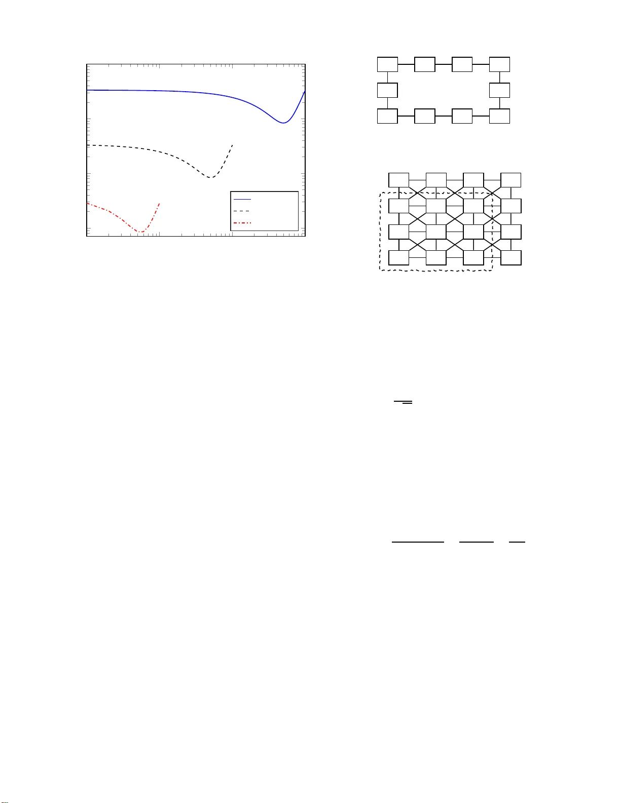
Distributed antennas must be phase-calibrated (phase-synchronized) for certain operations, such as reciprocity-based joint coherent downlink beamforming, to work. We use rigorous signal processing tools to analyze the accuracy of calibration protocol…
Authors: Erik G. Larsson
©2024 IEEE. Personal use of this material is permitted. Permission from IEEE mu st be obtain ed for all other uses, in any curr ent or future media, including reprinting/rep ublishing this m aterial for advertising or promotio nal purposes, creating new collective works, for resale o r redistribution to servers or lists, or reuse of any copyrig hted co mponent of this work in other works. This pape r will appear in the IEEE Transactions on Signal Processing, 202 4. TO APPEAR IN T HE IEEE TRANSACTIONS ON SIGN AL PROCESSING, 2024 1 Massi v e Synchrony in Distrib uted Antenna Systems Erik G. Larsson Abstract —Distributed a ntennas must be p hase-calibrated (phase-synchronized) fo r certain operations, such as reciproc ity- based joint coherent downlink beamforming, t o work. W e use rigoro us signal pro cessing too ls to a nalyze the accuracy of calibration protocols that are b ased on ov er -th e-air measur ements between antennas, with a focus on scalability aspects for lar ge systems. W e show that (i) for some who-measures-on-whom topologies, the errors in the calibration proce ss are unb ounded when the network gr ows; and (ii) despite that conclusion, it is optimal – irrespectiv e of the topology – to solve a single calibra- tion pr oblem fo r the en tire system and use t he result ev erywhere to sup port th e beamform ing. The analyses are exemplifi ed by in vestiga ting sp ecific topologies, in cluding li nes, rings, and two- dimensional surfaces. Index T er ms —phase calibration, synchronization, reciprocity , distributed antennas, MIMO, estimation, graph models, scalabil- ity I . I N T RO D U C T I O N A d istributed an tenna sy stem co nsists of access points that are spread out geogr aphically and cooper ate phase-coh erently on wireless co m municatio n or sensing tasks. This concep t is considered a main technology co mpon ent of the 6G physical layer, and variations of it appe a r und er the names distributed multiple-inp u t multiple-ou tput (MIMO) [1], network MIMO [2], u ser -centric MIMO [3], cell-fr e e massive MIMO [ 4], RadioW eaves [5], and radio stripes [6]. Each access point may have a single service antenn a, o r an array (pan el) of an tennas. At any point in time, each [ service] antenn a, n , is a ssoc ia ted with two comp lex-valued co efficients, T n and R n , that acco unt for hardware imperfectio ns and oscillator syn chroniza tio n er- rors, and which multiply the tran sm itted and received complex- baseband sign als. Herein , we will only be co ncerned w ith phase and set, fo r th e n th an tenna, T n = e − j t n and R n = e j r n for some p hase v alues t n and r n , defined mod 2 π . Th e conv ention with a minu s sign on t n facilitates an interpr etation of { t n , r n } in terms of time - delays [ 7]. T h e phase values { t n , r n } c o llectiv ely model two sep arate effects: E1. Geograph ically separ ated access points may have their own loca l oscillators th a t drive their r a dio-freq uency mixers. These oscillators ar e imperfect and noisy , and they differ from their nom in al spec ifications. This results in a time-varying shift between the oscillator phases at different access points. Unless all oscillators are locked to a c o mmon r eference u sin g a synch ronization cable – which is costly and even infeasible in so me deploy- ment scena r ios – this phase shift can fluctu a te and grow quickly . The author is with Link ¨ oping Uni versi ty , Dept. of Electrical Engineering (ISY), 581 83 Link ¨ oping, Sweden. E -mail: erik.g.la rsson@liu.se . This work was supported by ELLIIT , the KA W Foundati on, the Swedish Researc h Counc il (VR), and the REINDEER project of the European Union’ s Horizon 2020 research and innov ation program under grant agreement No. 101013425. E2. The transm it an d receive e lectronics branch at every antenna will ha ve a n unkn own phase lag that depen ds on manufactur ing variations and imperfectio ns in the circuits. This lag varies also varies with time, but slowly , once the equ ipment has warmed up. The exact time constant of the variation d epends o n the actual h ardware; in experim ental work repo rted in [8 ], the phase was substantially co nstant for hours. A. Calibration Over-the-Air Knowledge of c ertain relations between { t n , r n } is essential for the an tennas to coo perate phase-co herently . T h at calls for calibration in order to periodically estimate these values, or app ropriate fun ctions thereof. W e will be concern ed with calibration based on over -the-air measurements (in situ) be- tween pairs o f anten nas. W ithin an acc e ss point o ne relies on couplin g a mong the anten nas; between access points, one relies on radio-f requen cy pro pagation . Calibration within an access point may altern ativ ely be aid ed by dedicated internal calibration loops [9], [1 0], but that will be of no fur th er concern h ere. Our ana lysis herein will be agnostic to the a ctual origin of the variations in { t n , r n } , a n d to whether d ifferent antennas are co-located in a n array or geograp hically separated . But we em phasize that in p r actice, E1 p resents a much greater challenge than E2 , especially if the o scillators a re n ot locked to a co mmon refer e nce. Also, in practice, in a system with geogra p hically separated multiple- antenna access points it can be advantageo us to separ ate the p roblem s of calibratin g for E1 and E2: c alibrate the antennas within an ac cess point infrequ ently , and between the access poin ts mo re freque ntly . 1 B. Differ ent T ypes of Calib ration Distributed antenna system s can opera te with d ifferent pu r- poses, requiring different ty pes o f calibration [7]. Of particu lar interest are r eciprocity (R) calibr ation, and full (F) calibration. Here we give a con c ise exposition, to p rovide c o ntext. 1) Recipr ocity (R) calibration: T he system is R-calibrated if { t n + r n } are k nown, mo d 2 π , up to a commo n constan t for all n . R-calib ration enables recipr ocity-based , joint coheren t operation , relying on uplink pilots fo r downlink mu ltiuser MIMO beamfor ming. Over-the-air methods f or R-calibration use b idirectional measureme nts b etween antenna s, essentially measuring ( t n + r n ) − ( t n ′ + r n ′ ) for different pair s ( n, n ′ ) . This can be do ne for both co-lo cated arrays [ 8], [1 1]–[19] and for d istributed anten na systems [ 20]–[27]. Impor tan tly , over - the-air R-calibratio n works without know- ing a priori the pr opagatio n delay ( coupling ) between antenna s. 1 Alterna ti ve terms for [phase] calibrat ion between access points are phase synch r onizati on and phase alignment . Herein , we use the term calibr ation . ©2024 IEEE. Per sonal use of this material is permitted. Permission from IEEE mu st be obtain ed for all other uses, in any curr ent or future media, including reprinting/rep ublishing this m aterial for ad vertising or promotio n al purposes, creating new collective works, for resale o r redistribution to servers or lists, or reuse of any copyrig hted co mponent of this work in other works. This pape r will appear in the IEEE Transactions on Signal Processing, 202 4. TO APPEAR IN T HE IEEE TRANSACTIONS ON SIGN AL PROCESSING, 2024 2 Therefo re, there is n o difference in p rinciple betwe en R- calibrating the antennas in a single co -located array and [jointly] R-calibrating all anten n as in a distributed antenn a system – o ther tha n that in th e presen c e o f oscillator drifts, a distributed system would have to be re - calibrated mo re often. (The main effect in th is case is E1; f or more discussion of th e need for re- calibration in the p r esence of o scillator drifts, see [7], [ 28].) It is impor tant to appreciate the distinction between chan nel estimation and (R)- calibration . Both are req u ired f or joint coheren t, r eciprocity- based downlink beamf o rming to work. While chann el estimation in multiple-an tenna systems is we ll researched [3], the calibr ation problem has received less atten- tion. Y et, the latter is a difficult prob le m . I n time-d ivision d u - plexing (TDD) o p eration, chann e l estimates can be obtained, to any desired d egre e o f accu r acy , by sendin g uplink pilots with appr opriate len gth, power , and re use patterns. But over - the-air phase calibratio n requ ires th e tr ansmission of specially designed signals between ser vice antennas, wh ich breaks the TDD flow . 2) Full (F) calibration: The system is F-calibrated if { r n − r n ′ } , { t n − t n ′ } and { r n − t n } are k n own, mod 2 π , for all ( n, n ′ ) . V ariations exist, f or F-calibration only on rec e ive or transmit. F-calib r ation is stronger than R-calibr ation, and enables the use of geo metrically p arameterize d array mod els – facilitating fing erprintin g and directional ( in angle) b eamfor m - ing. F-ca lib ration implies R-c alibration, but n ot conversely . F-calibration ca n also be p erform ed over - the-air by per- forming m easurements between antennas [2 9], [30], but th is requires the prop agation delay between the antennas to be a priori known [7] – whic h can be ch allenging in a distributed antenna system. C. Specia lization to R-Ca libration In the r est of the paper we co nsider only R-calibr ation, although some o f the results also apply , mutatis mu tan dis, to other types of calibration. W e define, for each antenn a n , the p hase param eter φ n = t n + r n . Th e calib ration objective is then to obtain estimates, { ˆ φ n } , of { φ n } , fr om pairwise measuremen ts between an tennas. W e call { ˆ φ n − φ n } the [phase] estimation error s. In what follows, by system topo logy we refer to the gra ph that defines wh o measur es on whom – not to b e conf ounded with how antennas are in terconn e cted over backhau l, which is unimpo rtant h e re. D. Contributions and Pr eview of the Results The contribution o f th is paper is a rigorou s analysis of over- the-air ca lib ration, specifically addressing th ree qu estions: Q1. How accurately can { φ n } be estimated , fo r different system topo logies? Let N b e the total numb er of anten nas in th e system. What happ ens when N incr eases: do es the calibration pr oblem beco me easier or har der? W e show that for some topolo gies, V ar { ˆ φ n } can grow un- bound ed, f or all n . Th is hap pens, for examp le, f o r the line (radio stripe) to pology in Figure 1 , where a n tennas m ea- sure only on their immed iate n e ig hbors (Sectio n V -A). Ω 1 2 3 4 5 6 7 · · · N user A user B Fig. 1. L ine topology , where antennas perform calibrati on measurements on their immediate neighbors. T wo users A and B are also sho wn. Note that { φ n } , of course, are bo unded as they are o nly defined mod 2 π , so th is asympto tic statemen t means that errors aggr egate unfav orably . Q2. When perfo r ming recip r ocity-ba sed b eamfor m ing to a user , fro m a sub set – to be denoted Ω – o f th e antenn as, how sho uld calibration be perform ed? One may either (a) perfo rm R-calibration p roblem for th e whole system, or (b) perform R-calibration only in volving th e subset Ω . For example, co nsider Fig ure 1: user A is in th e field-of-v iew o f antennas 1 and 2; u ser B is in the field-of-v iew of anten n as 5 and 6. When calibrating for beamfor ming to A, will it be advantageous to (a) use calibration measureme n ts among all N antenn as, or (b) in volve on ly anten nas 1 and 2 in the calibration? From th e answer to Q1, o ne ma y intuit that option (b) is preferab le over (a). But we prove that (a ) is always better: irrespective of the top ology , it is o ptimal to solve a sing le calibration pr oblem for th e en tire system (Section IV) . Q3. For w h at topo logies is it p o ssible to achieve massive synchr ony , such th a t { Va r { ˆ φ n }} remain bounded , or e ven vanish, when N → ∞ ? While a complete characterization rem ains open , we hope that our analysis o ffers a starting point (Section VI). E. Related W ork The mo st c lo sely related work is th e ab ove-cited liter ature on R-calib ration [7], [8], [11]–[27]. No te th at d espite its title, [20] do es n o t conside r th e scalability a sp ects that we analyze herein. Our results a lso have som e conn ection to the writings on distributed synchro nization in comp lex and wire le ss net- works [3 1]–[36]. T hat liter ature, h owe ver, d eals with pr o tocols for synchron ization by b ilateral in teraction between d evices, whereas we co nsider calibration using centra lly pr o cessed measuremen ts. F . Notation Lowercase b old symbols a re colum n vectors, a n d up percase bold symbols are matrices. ( · ) ∗ represents the complex c o nju- gate. 0 is the all-ze r os vector/matrix. I is the iden tity matrix, and { e n } d enote the co lumns of I . For a set Ω , ¯ Ω den otes its complement. Gi ven a set of integers, Ω , E Ω denotes a matrix co mprising the columns { e n : n ∈ Ω } . ( · ) T denotes th e transpose of a vector or matrix, and ( · ) H denotes the Hermitian transpose. u is the vector of all on es: u = [1 , ..., 1] T . For a vector x , k x k is its nor m. F or a m atrix X , X − 1 is its inverse, det( X ) is its d eterminant, and [ X ] kl is its ( k , l ) elem ent. For ©2024 IEEE. Per sonal use of this material is permitted. Permission from IEEE mu st be obtain ed for all other uses, in any curr ent or future media, including reprinting/rep ublishing this m aterial for ad vertising or promotio n al purposes, creating new collective works, for resale o r redistribution to servers or lists, or reuse of any copyrig hted co mponent of this work in other works. This pape r will appear in the IEEE Transactions on Signal Processing, 202 4. TO APPEAR IN T HE IEEE TRANSACTIONS ON SIGN AL PROCESSING, 2024 3 a positive semidefinite matrix X , X 1 / 2 denotes its po siti ve semidefinite matrix squa r e r oot. For symmetric matrices X and Y of compatible d imensions, X < Y means th at X − Y is po sitive sem idefinite. I I . E S T I M A T I N G { φ n } F R O M M E A S U R E M E N T S A. Calibration Measur ement Mode l All ph ase values are defined mod 2 π . W e will assume that | φ n − φ n ′ | is small for all pairs ( n, n ′ ) , so that we can ig nore the mo d 2 π opera tio n w h en d ifferences between phase values are of concern . For R-calibration specifically , th is mean s tha t { t n + r n } differ only slightly for different n , suc h that the calibration only aims at corr ecting small residu al err o rs; for example, this is the c a se if a coarse calibr ation has b e e n undertaken previously . The N antenna s perf orm b idirectiona l over-the-air calibra - tion measurem e nts on one anoth er . Eac h pairwise interaction , say between anten nas n and n ′ , results in a measuremen t of φ n − φ n ′ , m od 2 π . If antenn as n m and n ′ m intercomm unicate in th e m th measurem ent, th is measur ement is, x m = φ n m − φ n ′ m + w m , (1) where w m is noise. All differences { φ n − φ n ′ } are small, and defined mod 2 π ; so are { x m } . The calibration objective is to estimate { φ 1 , ..., φ N } f r om { x 1 , ..., x M } , wher e M is the number of measu r ements. T his problem is ill-posed , irresp ectiv e of how large M is o r of the topolog y: by adding an a r bitrary constant to all { φ n } , none of { x m } changes. However , with e n ough measur ements, all { φ n } c a n be estimated up to a c o mmon , ad ditive constant. Throu g hout, the mea su rement n oise is the on ly source of random ness, and all expectation s are with respect to this n oise. W e assume that the measurem ent no ises { w m } are zero- m ean random variables with a k nown positive definite covariance matrix, Q = Cov { w } , (2) where w = [ w 1 , ..., w M ] T . In practice, one may explicitly per f orm p airwise measure- ments, as suggested by (1). Alternativ ely , one could have each antenn a bro adcast a synchron ization pilot that is re- ceiv ed by several n e ighbor ing anten nas simultaneou sly . In this case, ea ch bidir ectional measure m ent is co m pleted first when both inv olved node s h av e pe r formed th e ir bro adcast. For R- calibration of co -located a r rays, such b roadcasting strategies were developed in [18], [19]. Hereafter, the term “measure - ment” means an estimate of φ n − φ n ′ for an a ntenna pair ( n, n ′ ) , irrespective o f wh ether th is estimate is obtained by a single, direct b idirectional measu rement, averaging of multiple bidirection al measurem ents, or the use of a broad cast scheme. B. Graph Representation of the Mea sur ement Model W e repr esent the measuremen t topolog y by an undirec ted graph G , whose node s represen t the N antennas and whose edges represent th e M measuremen ts. Let B be the M × N in cidence matrix of G , wh ose m th row co rrespon ds to Ω ¯ Ω G G Ω Fig. 2. Example of G , G Ω , Ω , and ¯ Ω . Here N = 16 , N Ω = 6 , M = 25 and M Ω = 7 . the m th ed ge of G (the m th measu rement). For each m , [ B ] mn m = 1 and [ B ] mn ′ m = − 1 . All o ther elemen ts in the m th row of B are zero . Fur thermor e , let x = [ x 1 , ..., x M ] T and φ = [ φ 1 , ..., φ N ] T . Th en x = B φ + w . (3) W e d efine the pre- whitened measurem e n t vecto r x ′ = Q − 1 / 2 x = Q − 1 / 2 B φ + w ′ , (4) in which the effecti ve noise w ′ = Q − 1 / 2 w (5) has covariance m atrix Cov { w ′ } = I . The two cases of interest are: (a) All N antenn as are in volved in the calibration . In this case, we d enote the graph b y G and its incid ence matrix b y B , as alread y defin ed. The measure m ents are rep r esented by the vector x in (3), or equiv alently , the pre - whitened vector x ′ in ( 4). (b) Only a sub set, Ω , of the ante n nas are inv o lved in the calibration. The co rrespon d ing grap h is a subgraph of G , with N nod es and M Ω edges, where M Ω is the number of edges between nodes in Ω . W e d enote this subgrap h by G Ω , a n d its M Ω × N inc id ence matrix by B Ω . L et x Ω be the M Ω -vector com prising the measure ments amon g the antennas in Ω ; without loss of generality , we can assume that the M Ω last elements of x contain x Ω , such that x Ω = [ 0 I ] x . W e den ote the pr e-whitened me asurements by x ′ Ω = Q − 1 / 2 Ω x Ω , wh ere Q Ω = 0 I Q 0 I (6) is the M Ω × M Ω lower - right corner o f Q , that is, the p art of the noise covariance m atrix associated with the M Ω measuremen ts. W e assume that the n ominal graph G is connected . T he graph G Ω has N − N Ω isolated no des, corr espondin g to antennas that do no t participate. W e assume that the par t of G Ω correspo n ding to the N Ω antennas that actually par ticipate, is con nected. Figur e 2 shows an example. ©2024 IEEE. Per sonal use of this material is permitted. Permission from IEEE mu st be obtain ed for all other uses, in any curr ent or future media, including reprinting/rep ublishing this m aterial for ad vertising or promotio n al purposes, creating new collective works, for resale o r redistribution to servers or lists, or reuse of any copyrig hted co mponent of this work in other works. This pape r will appear in the IEEE Transactions on Signal Processing, 202 4. TO APPEAR IN T HE IEEE TRANSACTIONS ON SIGN AL PROCESSING, 2024 4 The Laplacian of the no minal gr aph, G , is B T B . T o accommo date a general n oise covariance matrix we d efine th e matrix L = B T Q − 1 B . (7) If Q = I , L red u ces to the standard graph L aplacian. If Q is diagona l, L becomes the Laplacian of a weig hted gr aph (with weights equ alling the recip rocal measurem ents variances). For general Q , th e matrix L is no t a conventional Laplacian matrix, but its n ullspace is the same as th at of the Laplacian B T B , and this is what is requ ir ed by the sub seq uent analysis. Since G is co nnected, the n ullspace of B T B , an d therefo re of L , is o ne-dimen sional and spanned by u [37]. Mo re specifically , b y a basis ch ange, L can be written as, L = [ u Z ] 0 0 0 Λ u T Z T , (8) where Λ is an ( N − 1) × ( N − 1) d iagonal matrix whose (positive) diagonal elements are th e no n-zero eigenvalues of L , and wher e Z is an N × ( N − 1) matrix wh ose column s are eigenv ectors of L and con stitute an or th onorm al basis f o r the o rthogo nal comp lement of u . Note th at (8) is similar to the eig en value decom p osition, but not iden tica l thereto as u does no t have u n it n o rm. The Laplacian of the weighted subg raph, G Ω , is given by B T Ω B Ω . Similar ly to a b ove, we define L Ω = B T Ω Q − 1 Ω B Ω , (9) which ag a in, is a (we ig hted) graph Lap lacian if Q is diago n al. The n u llspace of L Ω has dimension N ¯ Ω + 1 . Thro ugh a basis change, we can write, L Ω = [ u E ¯ Ω Z Ω ] 0 0 0 0 0 0 0 0 Λ Ω u T E T ¯ Ω Z T Ω , (10) for som e diago nal Λ Ω , wh ere Z Ω is an N × ( N Ω − 1) - dimensiona l matrix wh ose columns constitute an orthon o rmal basis of the orthog onal comp lement o f { u , E ¯ Ω } . Note that (10) is no t the eige nvalue de composition , since (amo n g oth ers) u a n d the column s of E ¯ Ω are not or thogon al. For future use, we note the fo llowing facts: • For Z , it h olds that Z T u = 0 , (11) Z T Z = I , (12) Z Z T = I − 1 N uu T (13) Z T LZ = Λ . (14) • For Z Ω , it h olds that Z T Ω u = 0 , (15) Z T Ω e n = 0 , n / ∈ Ω (16) Z T Ω Z Ω = I , (17) Z Ω Z T Ω = I − [ u E ¯ Ω ] u T E T ¯ Ω [ u E ¯ Ω ] − 1 u T E T ¯ Ω . (18) • Since G is co nnected, we must h av e M ≥ N − 1 . The nullspace of B is on e -dimension al and span ned by u : B u = 0 . The co lumn ran k of B is N − 1 . Th e c olumns of Z span the columns of B T and of ( Q − 1 / 2 B ) T . • Since the “ Ω -par t” of G Ω is connected, we must h av e M Ω ≥ N Ω − 1 . Further more, B Ω has column rank N Ω − 1 . Its nullspace is spanned by { u , E ¯ Ω } . The co lu mns of Z Ω span the column s of B T Ω and o f ( Q − 1 / 2 Ω B Ω ) T . C. Least-Squares Estimate of { φ n } in Case (a) In case (a), the least-squares estimate of φ , gi ven the pr e - whitened measurem ents in (4) o btained fr om the no minal graph G , is argmin φ k x ′ − Q − 1 / 2 B φ k 2 . (19) Since the co lumn space of ( Q − 1 / 2 B ) T is spanned by Z , φ can b e iden tified up to a vector prop o rtional to u . M ore precisely , (19) has th e solu tions ˆ φ = Z ˆ s + λ u , (20) where ˆ s = ( Z T B T Q − 1 B Z ) − 1 Z T B T Q − 1 x , (21) and λ is an ind eterminate scalar . While ˆ s is uniquely determined, λ is not. Fortunately , λ does not affect beamfo rming pe r forman ce ( Section II I). Hence, we can set λ = 0 . This yields th e uniqu e solution ˆ φ = Z ˆ s = Z ( Z T B T Q − 1 B Z ) − 1 Z T B T Q − 1 x . (22) Note, in passing, tha t among all solutions to (19), (2 2) is the one with the smallest k φ k . A d ir ect calculation y ields E { ˆ φ } = E { Z ( Z T B T Q − 1 B Z ) − 1 Z T B T Q − 1 ( B φ + w ) } = Z ( Z T B T Q − 1 B Z ) − 1 Z T B T Q − 1 · E B Z Z T + 1 N uu T φ + w = Z Z T φ , (23) Cov { ˆ φ } = Z ( Z T B T Q − 1 B Z ) − 1 Z T = Z ( Z T LZ ) − 1 Z T . (24) In the last step of (2 3), we used that B u = 0 and that E { w } = 0 . In ( 24), we addition ally used that Co v { w } = Q . Equation (23) implies that the par t o f ˆ φ that lies ou tside the un id entifiable (and uninter e stin g ) sub sp ace spann ed by u is unbiased . This mean s that (2 4) co mpletely quantifies the accur acy of ˆ φ . No te that Co v { ˆ φ } is r ank-de ficient – a consequen ce of the non- identifiability of λ . D. Monoton icity o f Cov { ˆ φ } in Case (a) For fixed N , b y adding m o re measureme n ts the accuracy of { ˆ φ } improves. T o see this, suppo se the nominal B is replaced by B ′′ = B ′ B , (25) ©2024 IEEE. Per sonal use of this material is permitted. Permission from IEEE mu st be obtain ed for all other uses, in any curr ent or future media, including reprinting/rep ublishing this m aterial for ad vertising or promotio n al purposes, creating new collective works, for resale o r redistribution to servers or lists, or reuse of any copyrig hted co mponent of this work in other works. This pape r will appear in the IEEE Transactions on Signal Processing, 202 4. TO APPEAR IN T HE IEEE TRANSACTIONS ON SIGN AL PROCESSING, 2024 5 for so m e B ′ that represents the additional m e asurements. Let Q ′′ be the no ise cov ariance o f the aug mented measureme nt set, such that Q is the lo wer-right N × N submatrix of Q ′′ . Explicitly , par tition Q ′′ accordin g to Q ′′ = " ¯ Q ˜ Q T ˜ Q Q # . (26) Let L ′′ = B ′′ T Q ′′− 1 B ′′ , (27) and let Z ′′ be the co unterpa r t of Z associated with L ′′ . By rewriting Q ′′− 1 using a Schur co mplement, we obtain (28), shown on top of the next page. Sin ce Q < Q − ˜ Q ¯ Q − 1 ˜ Q T , we h av e using Corollary 7.7 .4(a) of [38] th a t ( Q − ˜ Q ¯ Q − 1 ˜ Q T ) − 1 − Q − 1 < 0 . (29) Therefo re, the matrix in the middle o f the right han d side of (28) is positive sem idefinite, from which it follows th at the right hand side of ( 2 8) is positiv e sem idefinite (note its Gramian fo rm). W e con clude that L ′′ < L , w h erefro m it follows that Z ′′ T L ′′ Z ′′ < Z ′′ T LZ ′′ . By apply in g ag a in Corollary 7.7 .4(a) of [38], w e find that ( Z ′′ T LZ ′′ ) − 1 < ( Z ′′ T L ′′ Z ′′ ) − 1 . (30) The nu llspaces o f L and L ′′ are one-dimen sio nal and spanned by u . Therefor e, Z and Z ′′ have the same c olumn space. It fo llows tha t there exists an ( N − 1) × ( N − 1) m atrix Ψ such that Z ′′ Ψ = Z (31) Ψ T Ψ = ΨΨ T = I . (32) Therefo re, Z ( Z T LZ ) − 1 Z T − Z ′′ ( Z ′′ T L ′′ Z ′′ ) − 1 Z ′′ T = Z ′′ Ψ ( Ψ T Z ′′ T LZ ′′ Ψ ) − 1 Ψ T Z ′′ T − Z ′′ ( Z ′′ T L ′′ Z ′′ ) − 1 Z ′′ T = Z ′′ ( Z ′′ T LZ ′′ ) − 1 Z ′′ T − Z ′′ ( Z ′′ T L ′′ Z ′′ ) − 1 Z ′′ T = Z ′′ ( Z ′′ T LZ ′′ ) − 1 − ( Z ′′ T L ′′ Z ′′ ) − 1 Z ′′ T < 0 , (33 ) where in the last step w e used (30). That is, the difference between Co v { ˆ φ } with out the additional measur ements, and Cov { ˆ φ } with those m easuremen ts, is positive semidefin ite. E. Least-Squ ar es Estimate of { φ n } in Case (b) In case (b), the co rrespon d ing least-squar es prob lem is argmin φ k x ′ Ω − Q − 1 / 2 Ω B Ω φ k 2 . (34) Problem (34) has the so lu tions ˆ φ = Z Ω ˆ s Ω + λ u + X n / ∈ Ω λ n e n , (35) where ˆ s Ω = ( Z T Ω B T Ω Q − 1 Ω B Ω Z Ω ) − 1 Z T Ω B T Ω Q − 1 Ω x Ω , (36) and λ and { λ n } are ind eterminate scala r s that we will set to z e r o. Th e mean and covariance can be f ound v ia a similar calculation as in Section II-C, using the above-established facts about L Ω , Z Ω , an d B Ω : E { ˆ φ } = Z Ω Z T Ω φ , (37) Cov { ˆ φ } = Z Ω ( Z T Ω L Ω Z Ω ) − 1 Z T Ω . (38) Note th at Va r { ˆ φ n } f o r n ∈ Ω is not ne cessarily larger in case (b) than in case ( a), e ven thoug h in case (a) we have more measuremen ts, because in case (a) the r e are more identifiable parameters. I I I . B E A M F O R M I N G G A I N A N A LY S I S Next we examine the impact of estimation errors in { ˆ φ n } on joint coh erent downlink beamformin g per f ormanc e, when targeting a sp e cific point (fo cal spot) in sp ace with recipr o city- based bea mformin g. The b eamfor m ing is performed by the antennas in the set Ω . T o keep th e analy sis clean, we re stric t the discussion to the beamfo rming of a mon o chrom a tic (sinusoidal) signal with some given car rier frequency . The argument extend s directly to any signal whose ban d width is less tha n the channel coh erence bandwidth (reciproc a l excess d elay). 2 Also, nothin g prevents the app lication o f the analysis to multiple narrowband sig n als that are adjac ent in the f requen cy domain. Let h n be the channel fr equency response (co mplex-baseba n d channe l gain) at the carrier freq uency of concern, between the n th antenna and the fo cal spot, and let a n be the respective beamfor ming weight ap plied by th e n th antenn a. Suppose th at the above-described estimates { ˆ φ n } ar e used to p r e-comp ensate { a n } wh en perf orming the beamfor m ing. The effectiv e c h annel to the f ocal spot is then g = X n ∈ Ω h n a n e j ˆ φ n e − j φ n . (39) The co rrespon d ing beamf o rming (power) gain is | g | 2 . Addin g a co m mon co nstant to all { ˆ φ n } d oes n ot affect | g | , wh ich is why we can safely set λ = 0 and λ n = 0 in Sectio n II. A. Beamforming fo r Constructive Interfer ence If { φ n } are per fectly known, then | g | can b e made to scale with N , by tak ing the angle of a n to align with that of h ∗ n , causing co nstructive interference at the foca l spot. Th is gives the standar d coh erent array g a in . If { φ n } are only imperf ectly known, the ar r ay g ain dete- riorates. In prac tice , accur a te k nowledge is not critical. For example, suppose | h n | = 1 and that { φ n } for half of the antennas are perfec tly known, but that { φ n } for the other antennas are off by δ radians. The r elativ e loss in | g | 2 is then | 1 + 1 | 2 / | 1 + e j δ | 2 . Even if δ = π / 2 ( 9 0 ◦ ) th e loss is only 3 dB. But beyond 90 ◦ errors, the array g ain qu ickly ev ap o rates. W e omit a detailed analysis and in stead focus o n the mo r e interesting case of null-steerin g, n ext. 2 T echnica lly , a finite exc ess-dela y assumption is inconsistent with an array apertur e that grows to infinity . In pract ice, signals origina ting at antennas fart her and fart her awa y would be at tenua ted more and more strongly , e ven tuall y contribut ing neglig ibly to the channel response. ©2024 IEEE. Per sonal use of this material is permitted. Permission from IEEE mu st be obtain ed for all other uses, in any curr ent or future media, including reprinting/rep ublishing this m aterial for ad vertising or promotio n al purposes, creating new collective works, for resale o r redistribution to servers or lists, or reuse of any copyrig hted co mponent of this work in other works. This pape r will appear in the IEEE Transactions on Signal Processing, 202 4. TO APPEAR IN T HE IEEE TRANSACTIONS ON SIGN AL PROCESSING, 2024 6 L ′′ − L = B ′′ T Q ′′− 1 B ′′ − B T Q − 1 B = B ′′ T Q ′′− 1 B ′′ − B ′′ T 0 I Q − 1 0 I B ′′ = B ′′ T Q ′′− 1 − 0 I Q − 1 0 I B ′′ = B ′′ T " I − ¯ Q − 1 ˜ Q T 0 I # " ¯ Q − 1 0 0 ( Q − ˜ Q ¯ Q − 1 ˜ Q T ) − 1 # I 0 − ˜ Q ¯ Q − 1 I − 0 I Q − 1 0 I ! B ′′ = B ′′ T " I − ¯ Q − 1 ˜ Q T 0 I # " ¯ Q − 1 0 0 ( Q − ˜ Q ¯ Q − 1 ˜ Q T ) − 1 − Q − 1 # I 0 − ˜ Q ¯ Q − 1 I B ′′ (28) B. Beamforming fo r Destructive Interference W ith nu ll-steering, { a n } ar e selected such that the signals from different antennas interfer e destructively at the focal sp ot: X n ∈ Ω h n a n = 0 , (40) attempting to m ake g = 0 . T his is the opera tio nal principle of zero-fo rcing beam formin g fo r multiuser MI M O [3 9], [40]. T o analyze the beamfo rming gain in the presence of p h ase estimation errors, consider first case (a). Recall th at { ˆ φ n − φ n } have nonz e ro mean b ecause of the no n-identifiab ility of the estimation pr oblem; see (23). For a n alysis purp oses, it will prove u seful to intro duce the following in te r mediate quantities: ˜ φ n = ˆ φ n − φ n + ¯ φ, (41) where we defin ed the av erage of th e p hase values, ¯ φ = 1 N N X n =1 φ n = u T φ N . (42) One can think of { ˜ φ n } as the “zero -mean part” o f the estimation errors, because E { ˜ φ n } = 0 fo r all n . T o see why this is so, let ˜ φ = [ ˜ φ 1 , ..., ˜ φ N ] T and note that from ( 13), (23), (41) and (42) we have that E { ˜ φ } = Z Z T φ − φ + uu T N φ = 0 . (43) W e now re-expr e ss the effective ch annel in (39) in terms o f { ¯ φ n } a n d { ˜ φ n } : g = X n ∈ Ω h n a n e j ˆ φ n e − j φ n = e − j ¯ φ X n ∈ Ω h n a n e j ˜ φ n ≈ e − j ¯ φ X n ∈ Ω h n a n (1 + j ˜ φ n ) = e − j ( ¯ φ − π / 2) X n ∈ Ω h n a n ˜ φ n , (44) where in the third step we perform ed a first-ord e r T aylor expansion, e × ≈ 1 + × . This expansion is justified since { ˜ φ n } have zero mean, and in the limit of weak me a surement no ise they would fluctu ate only slightly . In the last step of (44) we used (4 0). Next, consider case (b). T he analysis is analogous to th e one for case (a) , but with ¯ φ re-d efined. Specifically , in co n trast to (42), now we set ¯ φ = 1 0 T u T E T ¯ Ω [ u E ¯ Ω ] − 1 u T E T ¯ Ω φ , (45) and no te tha t for n ∈ Ω , it ho lds tha t e T n [ u E ¯ Ω ] = [1 0 T ] ; therefor e, for n ∈ Ω , we have e T n [ u E ¯ Ω ] u T E T ¯ Ω [ u E ¯ Ω ] − 1 u T E T ¯ Ω φ = ¯ φ. (46) Using (18) and (37) we then find th at f or n ∈ Ω , E { ˆ φ n } = e T n Z Ω Z T Ω φ = φ n − ¯ φ. (47) Letting, as befo re, ˜ φ n = ˆ φ n − φ n + ¯ φ, we h ave tha t E { ˜ φ n } = φ n − ¯ φ − φ n + ¯ φ = 0 (48) for n ∈ Ω . This m eans that the f ormula for the effecti ve channel, (4 4), applies to ca se (b ), as well. Consequently , we have for b oth cases (a) and (b), that g ≈ e − j ( ¯ φ − π / 2) · v T ˜ φ , (49) where v is an N -vector whose compon ents are v n = ( h n a n , n ∈ Ω 0 , otherwise . (50) In eithe r case, ˜ φ h a s zero mean , and covariance Cov { ˜ φ } = Cov { ˆ φ } , given by (24) and (38), respectively . It follows th a t E { g } ≈ 0 , (51) V ar { g } ≈ v T Cov { ˆ φ } v ∗ = v H Cov { ˆ φ } v , (52) with the respective (real-valued) cov ariance matrices in ( 24) and (3 8) inserted for Co v { ˆ φ } . I V . B E A M F O R M I N G G A I N C O M PA R I S O N Hencefor th , we are only in te r ested in null-steering. The variance of g , Va r { g } , quantifies th e beamfor ming accura cy in terms of h ow m uch power inad vertently reaches the focal point, f o r an arbitrary ch oice o f beam f orming weights { a n } satisfying (40). (Th e smaller the variance, the better the ©2024 IEEE. Per sonal use of this material is permitted. Permission from IEEE mu st be obtain ed for all other uses, in any curr ent or future media, including reprinting/rep ublishing this m aterial for ad vertising or promotio n al purposes, creating new collective works, for resale o r redistribution to servers or lists, or reuse of any copyrig hted co mponent of this work in other works. This pape r will appear in the IEEE Transactions on Signal Processing, 202 4. TO APPEAR IN T HE IEEE TRANSACTIONS ON SIGN AL PROCESSING, 2024 7 accuracy .) W e will now com pare this v ariance, f or gi ven { a n } , between th e following two cases: (a) Beamforming is under taken b y the sub set Ω of th e anten- nas, a nd { ˆ φ n } are o btained fr o m calibration me a su rements among all N a n tennas, that is, from G . (b) Beamformin g is undertaken by the subset Ω o f the antennas, but { ˆ φ n } are obtained on ly from c alibration measuremen ts among a ntennas th at participate in th e beamfor ming, that is, from G Ω . First note f rom ( 5 0) that (40) can be eq uiv alently written as P n v n = 0 ; th at is, using vector notation , u T v = 0 . (53) Also, note th at the con straint th at v n = 0 for n / ∈ Ω in (50) can be expressed as e T n v = 0 , n / ∈ Ω . (54) T aken to g ether, this m eans that the set o f po ssible beamf orm- ing weights { a n } is defined by the set of N -vectors v th a t satisfy (53) and (54). Since the columns of Z Ω span the orthog onal complement of the sp a ce span ned by { u , E ¯ Ω } , we know that for an ar bitrary vector v that satisfies ( 5 3)–(54), there exists a un ique ( N Ω − 1) -vector p such that v = Z Ω p . (55) In case (a), the variance (5 2) is given by the qu adratic form V a = v H Z ( Z T LZ ) − 1 Z T v = p H Z T Ω Z ( Z T LZ ) − 1 Z T Z Ω p = p H K a p , (56) where we defin ed the kernel, K a = Z T Ω Z ( Z T LZ ) − 1 Z T Z Ω . (57) In case (b), the variance is V b = v H Z Ω ( Z T Ω L Ω Z Ω ) − 1 Z T Ω v = p H Z T Ω Z Ω ( Z T Ω L Ω Z Ω ) − 1 Z T Ω Z Ω p = p H ( Z T Ω L Ω Z Ω ) − 1 p = p H K b p , (58) where K b = ( Z T Ω L Ω Z Ω ) − 1 . (59) W e ar e now going to establish th a t V b ≥ V a for any p , from w h ich it then follows that V b ≥ V a for any v tha t satisfies (53)–(54), an d therefor e f or any { a n } that satisfy (40). Clearly , this is the case if w e can demonstrate that K b < K a . Fro m Corollary 7.7 .4(a) of [3 8], we know th at K b < K a if an d on ly if K − 1 a < K − 1 b . Th erefore, the sou ght-after resu lt follows if we can show that K − 1 a − K − 1 b < 0 . The co mplication in the analysis lies in the ran k-deficiency of L and L Ω . T o tackle this, note that Z and [ Z Ω E ¯ Ω ] have the same colu mn space; henc e, th ere exists an ( N − 1) × ( N − 1 ) matrix Ψ such that Z Ψ = [ Z Ω E ¯ Ω ] , (60) Ψ T Ψ = ΨΨ T = I . (61) By multiplying (60) from the lef t by Z T Ω and fr o m th e rig ht by Ψ T , we find that Z T Ω Z = [ I 0 ] Ψ T . (62) It f o llows that K a = Z T Ω Z ( Z T LZ ) − 1 Z T Z Ω = I 0 Ψ T Z T LZ − 1 Ψ I 0 = I 0 Z T Ω E T ¯ Ω L Z Ω E ¯ Ω − 1 I 0 = Z T Ω LZ Ω − Z T Ω LE ¯ Ω ( E T ¯ Ω LE ¯ Ω ) − 1 E T ¯ Ω LZ Ω − 1 , (63) where in the last step, we used the block matrix in version lemma. 3 W e have already assum ed that th e edg es of the grap h are ordered such that B = B ′′′ B Ω , ( 64) for som e B ′′′ . Define ∆ = L − L Ω = B T Q − 1 B − B T Ω Q − 1 Ω B Ω = B T Q − 1 B − B T 0 I Q − 1 Ω 0 I B = B T Q − 1 − 0 I Q − 1 Ω 0 I B . (65) By recalling that Q Ω is the lower-right N Ω × N Ω submatrix of Q , rewriting Q − 1 using a Schur complemen t, and perform ing a calculatio n similar to that in (28), we conclu de that ∆ < 0 . Also, becau se of ( 10), L Ω E ¯ Ω = 0 . (66) Using (59) and (63), the difference between the in verse kernels can then be written, K − 1 a − K − 1 b = Z T Ω LZ Ω − Z T Ω LE ¯ Ω ( E T ¯ Ω LE ¯ Ω ) − 1 E T ¯ Ω LZ Ω − Z T Ω L Ω Z Ω = Z T Ω L − L Ω − LE ¯ Ω ( E T ¯ Ω LE ¯ Ω ) − 1 E T ¯ Ω L Z Ω = Z T Ω ∆ − ( L Ω + ∆ ) E ¯ Ω ( E T ¯ Ω ( L Ω + ∆ ) E ¯ Ω ) − 1 · E T ¯ Ω ( L Ω + ∆ ) Z Ω = Z T Ω ∆ − ∆ E ¯ Ω ( E T ¯ Ω ∆ E ¯ Ω ) − 1 E T ¯ Ω ∆ Z Ω = Z T Ω ∆ 1 / 2 I − ∆ 1 / 2 E ¯ Ω ( E T ¯ Ω ∆ E ¯ Ω ) − 1 E T ¯ Ω ∆ 1 / 2 · ∆ 1 / 2 Z Ω . (67) 3 Whene ver the in ver ses exi st [38 , Sec. 0.7.3], A B C D − 1 = ( A − B D − 1 C ) − 1 A − 1 B ( C A − 1 B − D ) − 1 ( C A − 1 B − D ) − 1 C A − 1 ( D − C A − 1 B ) − 1 . ©2024 IEEE. Per sonal use of this material is permitted. Permission from IEEE mu st be obtain ed for all other uses, in any curr ent or future media, including reprinting/rep ublishing this m aterial for ad vertising or promotio n al purposes, creating new collective works, for resale o r redistribution to servers or lists, or reuse of any copyrig hted co mponent of this work in other works. This pape r will appear in the IEEE Transactions on Signal Processing, 202 4. TO APPEAR IN T HE IEEE TRANSACTIONS ON SIGN AL PROCESSING, 2024 8 The matr ix in side the paren thesis after the last eq uality in (67) is th e o r thogon al pro jection onto th e o rthogo nal com p lement of the c o lumn sp a ce of ∆ 1 / 2 E ¯ Ω . Therefor e , (67) is po siti ve semidefinite, and the desire d result f ollows: the beamfo rming accuracy in case (a) is always b etter than, or equ al to , that in case (b ). As a final remark, we comm e nt on the implicatio ns of monoto nicity (Section II-D) on the beamform ing gain, wh en adding mo re measuremen ts. Con sider case (a). Let V a be the nominal variance, and V ′′ a be th e variance after th e addition of supp lementary measurem ents. From (3 3) and (56) it is th en immediate that V ′′ a ≤ V a , for any perm issible { a n } . This effect must n ot, of course, b e co nflated with the co nclusion fro m the compariso n between cases (a) and (b ) derived above. V . E X A M P L E S The estimation errors in { ˆ φ n } ca n grow fast when scaling up the network. Y et, the beam formin g a c curacy , for any subset Ω , is alw ays better wh en all measurements ar e used. T his is best illustra te d thro u gh th e stud y of some spe c ia l cases. In all examples, we assume that the measuremen t noises are uncorr elated, and set the noise variance to one: Q = I . (In the nu merical illustrations, we scale Q .) In this case, L is th e standard L aplacian. Whe n readin g the examples, it is usefu l to keep in mind its eq uiv a len t definitio n: L = D − A , where A is the graph ad jac ency m atrix ( [ A ] nn ′ = 1 if n and n ′ are connected , an d zero othe r wise) and D is a diag onal matrix with Au on its d iagonal. A. Linear (Radio S tripe) T opology First we co nsider the line ( r adio stripe) topo logy in Figure 1, where me a surements ar e only conducted b etween neig hborin g antennas. The Laplacian is imm ediate fr o m its definition: L = 1 − 1 0 · · · · · · · · · · · · 0 − 1 2 − 1 0 . . . 0 − 1 2 − 1 . . . . . . . . . 0 . . . . . . . . . . . . . . . . . . . . . . . . . . . . . . 0 . . . . . . . . . − 1 2 − 1 0 . . . 0 − 1 2 − 1 0 · · · · · · · · · · · · 0 − 1 1 . (68) Let y n = cos 1 2 ( n − 1) π N cos 3 2 ( n − 1) π N . . . cos 2 N − 3 2 ( n − 1) π N cos 2 N − 1 2 ( n − 1) π N , (69) for n = 1 , ..., N . A direct but tedious calculation, or the use of results from [41], sh ows that { y n } ar e m u tually ortho gonal and tha t they are eigenvectors of L : Ly 1 = 0 (70) Ly n = [ Λ ] ( n − 1)( n − 1) y n , n = 2 , ..., N , (71) y T n y n ′ = 0 , n 6 = n ′ , (72) where th e corresp o nding e ig en values are [ Λ ] ( n − 1)( n − 1) = 4 sin 2 ( n − 1) π 2 N . (73) Note that the first eigenv alue is ze ro; actu ally , y 1 = u . T aken together, this means that Z can be written as Z = [ z 2 · · · z N ] where z n = y n k y n k . (74) In par ticular, (14) ho lds. It f o llows that, Cov { ˆ φ } = Z ( Z T LZ ) − 1 Z T = N X n =2 z n z T n [ Λ ] ( n − 1)( n − 1) = 1 4 N X n =2 y n y T n sin 2 ( n − 1) π 2 N k y n k 2 . (75) Now u se (6 9) to write th e n th diag onal element o f Cov { ˆ φ } as V ar { ˆ φ n } = 1 4 N X n ′ =2 cos 2 (2 n − 1) ( n ′ − 1) π 2 N sin 2 ( n ′ − 1) π 2 N k y n ′ k 2 . (76) The right hand side of (76) can be lower - b ound ed by reta in ing only the first two terms, for which n ′ = 2 and n ′ = 3 . (Keeping o nly the first ter m turn s ou t to be insufficient.) The sum of th e num e rators corre sponding to n ′ = 2 and n ′ = 3 is lower - bound ed, unif ormly over n , as follows: cos 2 (2 n − 1) π 2 N + cos 2 (2 n − 1) π N = 1 2 h 1 + cos (2 n − 1) π N + 2 co s 2 (2 n − 1) π N i = 1 2 1 + 1 2 cos (2 n − 1) π N 2 + 7 8 cos 2 (2 n − 1) π N ≥ 1 8 . (77) From (6 9) it is im mediate that k y n k 2 ≤ N , n = 1 , ..., N . (78) Since sin( x ) ≤ x fo r x ≥ 0 , the denomin ator of th e terms inside the su m of (76) for n ′ = 2 and n ′ = 3 is upper-boun d ed by , sin 2 ( n ′ − 1) π 2 N k y n ′ k 2 ≤ π N 2 N = π 2 N . (79) Putting the se boun ds to gether we find that u niform ly over n , V ar { ˆ φ n } ≥ N 32 π 2 . (80) ©2024 IEEE. Per sonal use of this material is permitted. Permission from IEEE mu st be obtain ed for all other uses, in any curr ent or future media, including reprinting/rep ublishing this m aterial for ad vertising or promotio n al purposes, creating new collective works, for resale o r redistribution to servers or lists, or reuse of any copyrig hted co mponent of this work in other works. This pape r will appear in the IEEE Transactions on Signal Processing, 202 4. TO APPEAR IN T HE IEEE TRANSACTIONS ON SIGN AL PROCESSING, 2024 9 10 0 10 1 10 2 10 3 10 − 4 10 − 3 10 − 2 10 − 1 antenna index ( n ) V ar { ˆ φ n } N = 1000 N = 100 N = 10 Fig. 3. Va r { ˆ φ n } as function of antenna index n , for dif ferent total numbers of antennas, N , for the line (radio stripe ) topology in Figure 1, for Q = 10 − 4 · I . Note the logari thmic scale; the minimum occurs when n = N/ 2 . This shows that the smallest v alue amon g Va r { ˆ φ n } → ∞ as N → ∞ (r ather q uickly). De sp ite th is, we know , fro m the analysis in Section IV, th at the beamf orming accuracy for any fixed subset Ω canno t decrease when inclu ding mor e anten n as in the calibration p rocess. In th is pa r ticular example with a line topolog y , it turn s o ut that K a = K b (see below), but we will see an example later (Sectio n V -C) where K b is strictly larger than K a . T o see why K a = K b in th e present example, consider first the case that Ω = { 1 , ..., N Ω } , and lo o k at the p enultimate line of (67). Let Ψ = ∆ − ∆ E ¯ Ω ( E T ¯ Ω ∆ E ¯ Ω ) − 1 E T ¯ Ω ∆ and note that Ψ E ¯ Ω = 0 ; likewis e, Ψ u = 0 . A lso note th at ∆ has zer os in its ( N Ω − 1 ) × ( N Ω − 1) uppe r-left cor ner; so has Ψ . Sinc e u is linearly independent of the column s of E ¯ Ω , the only possibility is Ψ = 0 , which, by (67), implies K a = K b . T he case wh en Ω con sists of a different set of co nsecutive indices can be han dled similarly . Figure 3 shows Va r { ˆ φ n } as function of n , for some different values of N . The largest variances occ ur at th e ends o f the stripe. When N → ∞ , th e smallest among { Var { ˆ φ n }} (wh ich, as seen in the figu re, is in the m iddle of the strip e) – and therefor e all of them – g row without boun d. W e remind the reader ab out th e point mad e earlier regarding arithmetic mod 2 π . Also, we stress that the inequa lity (80) is not tight at all; its on ly p urpose is to show the unboun dedness. B. Ring T op ology A variation on th e previous examp le is a r ing topology , obtained from the line topolo gy by co nnecting n o des 1 and N (Figure 4). The Laplacian b e comes a circulan t matr ix, which can be d iagonalized using the discrete Fourier transfo rm [42]. Because of the symme tr y , the eigen values of L appe a r in pairs and the eigenvectors appear in complex-conju gated p airs, such 1 2 3 4 5 6 7 8 · · · N Fig. 4. Ring topology , where ev ery antenna performs measurements on its two neighbo rs. Ω 1 2 3 · · · 4 5 6 · · · 7 8 · · · · · · · · · · · · · · · N Fig. 5. Large-inte llige nt-surf ace topology , where each anten na performs mea- surements on its north-south , east-west, southeast-northwe st and southwest- northea st closest neighbors. that a p prop r iate linear com binations there o f yield real-valued eigenv ectors. Am o ng these eig en vectors, on e is z = 1 √ N 1 cos(2 π / N ) cos(2 · 2 π / N ) . . . cos(( N − 1)2 π / N ) , ( 81) which has un it norm , k z k = 1 , and corre sponding eigenv alu e 4 sin 2 ( π / N ) . (One can alter natively find this eig e n vector from results in [41].) In this example all nodes are statistically iden tical and a calculation somewhat similar to, but simpler than, th e one in Section V -A (we leav e the details to the reader) shows that for any n , V ar { ˆ φ n } ≥ 1 / N 4 sin 2 ( π / N ) ≥ 1 / N 4 π 2 / N 2 = N 4 π 2 . (82 ) Thus as N → ∞ the rin g exhib its th e same behavior as the line topo logy: the variances grow withou t bou nd. C. Lar ge-In telligent-Surface T opo logy In the next example we consider a large intelligent surface, 4 en visioned by many as a main physical- lay er solu tion fo r 6G [5], [4 4]. Th e idea is to c over a large surface (f or example, a wall o r ceiling of a building) by antennas that may be, f or aesthetic reason s, phy sically in tegrated into the surface itself. W e assume, for the example, that eac h antenna can p erform calibration measurem e nts on its eigh t closest neighb o rs (except for the anten nas on the b order ) , as shown in Figur e 5. The 4 A large intellig ent surface is not to be confuse d with a reflec ting inte llige nt surfac e (RIS), also kno wn as an intelli gent reflect ing surface (IRS). The use of a RIS (IRS) entai ls its o wn calibrat ion challe nges [43], but they are of a total ly dif ferent kind and unrelat ed to the material presented herein. ©2024 IEEE. Per sonal use of this material is permitted. Permission from IEEE mu st be obtain ed for all other uses, in any curr ent or future media, including reprinting/rep ublishing this m aterial for ad vertising or promotio n al purposes, creating new collective works, for resale o r redistribution to servers or lists, or reuse of any copyrig hted co mponent of this work in other works. This pape r will appear in the IEEE Transactions on Signal Processing, 202 4. TO APPEAR IN T HE IEEE TRANSACTIONS ON SIGN AL PROCESSING, 2024 10 10 1 10 2 10 3 2 4 6 8 · 10 − 5 number of antennas ( N ) V ar ( ˆ φ 1 ) (i) using all N antennas (ii) using antennas in Ω Fig. 6. For the topology in Figure 5, and Q = 10 − 4 · I : (i) Va r { ˆ φ 1 } when using all av ailable calib ration m easurement s; (ii) Va r { ˆ φ 1 } when using only the calibra tion measurements among antennas in Ω , consisting of the nine antenna s in the 3 × 3 lower left corner of the surface. 10 1 10 2 10 3 0 0 . 2 0 . 4 number of antennas ( N ) eigen value ratio Fig. 7. For the topology in Figure 5: the large st eigen valu e of K b − K a relati ve to the largest eigen val ue of K b . Laplacian is easily written d own but analy sis in closed for m , beyond th e g eneral formulas already obtained, is cu mbersom e. Figure 6 shows the fo llowing: (i) the estimation er ror variance for the an tenna in the lower- left corner (numb er 1 in Figure 5), Va r { ˆ φ 1 } , for case (a), when using all M calibration measurem e nts, and (ii) Va r { ˆ φ 1 } for case (b) when using only the M Ω calibration measuremen ts among anten nas in a subset Ω , con sisting of the nine an tennas in the 3 × 3 lower left cor n er of the surface. W e make the following o bservations: • Va r { ˆ φ 1 } in case (a) in creases when using mo r e antennas, though not as fast as for the line top ology ( cf. (8 0)). W e conjecture that the variance is unb o unded wh en N → ∞ . • Va r { ˆ φ 1 } in case (b) is, of cou rse, indepen dent o f N . Next, Figure 7 shows th e largest possible imp rovement in beamfo rming accuracy when u sing all antennas for cal- ibration, comp ared to when using only the antenna s in Ω , quantified via the largest eigenv a lu e of K b − K a rela- ti ve to the la rgest e igenv alu e of K b . Th is is the largest value that V b − V a can attain relative to the largest pos- sible value that V b can attain, for any u nit-nor m v . ( Note that k v k 2 = v H v = p H Z T Ω Z Ω p = p H p = k p k 2 .) A sig n ifi- cant improvement in perfo rmance when beamformin g from antennas in Ω can be achieved b y using calibration measure- ments from an te n nas outside of Ω . But the ga in levels off quickly . Beyond N = 16 the curve is almo st flat so th ere is no po int in practice in going b eyond the 4 × 4 lower-left corner . D. Complete Graph T opology W e end with an exposition of the situation when a ll N antennas m easure on all others. In this case, G is a co mplete graph with M = N ( N − 1) / 2 ed ges. The Laplacian is L = N I − uu T . (83) Recalling that u T Z = 0 , we find th at Cov { ˆ φ } = Z ( Z T LZ ) − 1 Z T = 1 N Z Z T . (84) The variance of ˆ φ n , f o r an arbitrary n , fo llows as, V ar { ˆ φ n } = e T n Cov { ˆ φ } e n = 1 N e T n Z Z T e n = 1 N e T n I − 1 N uu T e n = 1 N 1 − 1 N = 1 N − 1 N 2 . (85) When add ing more an d mor e antenn as, this variance go es to zero: Va r { ˆ φ n } → 0 as N → ∞ , uniform ly over n . This is a consequen ce of the d e nse topo logy , and the conclu sion is the opposite of that for the o ther topolo gies discu ssed above. In the present example, the n u mber of u nknowns is prop o rtional to N , but th e num ber of mea su rements is pr oportio n al to N 2 , making the prob lem more and m ore well-con ditioned as N increases. V I . M A S S I V E S Y N C H RO N Y Returning to question Q3 asked in Section I-D, what top olo- gies enable massi ve synch rony in the sen se that { Va r { ˆ φ n }} remain boun ded, o r e ven v a n ish, when N → ∞ ? For the complete graph (Section V -D), all variances tend to zero. But for the line to polog y , in contrast (Section V -A) all variances tend to in finity . It ap pears plau sible that the comp le te gr aph could be “thinned o ut” quite substantially bef ore en counterin g this ph enomen on, but it is u nclear exactly h ow mu ch. One ob servation is that the average variance can be written in terms of the L aplacian eigenv alues: 1 N N X n =1 V ar { ˆ φ n } = 1 N T r n Cov { ˆ φ } o = 1 N T r n Z Λ − 1 Z T o = 1 N T r n Λ − 1 Z T Z o = 1 N T r Λ − 1 = 1 N N − 1 X n =1 1 [ Λ ] nn . (86) For a tree topolo gy , an d for unco rrelated, homoskedastic noise ( Q = I ) on e c an use [45, Theorem 4.3 ] (see also [46]) to write the rig ht hand side of (86) as a constant times th e av erage distan c e between pairs of no des in G . For an arbitra r y topolog y , mono tonicity (Sectio n II- D) then gives an up per bound o n the a verage variance in terms o f the average distance of a spann in g tree. ©2024 IEEE. Personal use of this material is permitted. Permission from IEE E must be obtained for all other uses, in any current or future media, including reprinting /republishing this material for advertising or promotional purposes, creating new collective works, for resale or redistribution to servers or lists, or reuse of any copyrighted component of this work in other works. This paper will appear in the IEEE Transactio ns on Signal Processing, 2024. TO APPEAR IN T HE IEEE TRANSACTIONS ON SIGN AL PROCESSING, 2024 11 Whether stronger results can be established rem ains o p en. These questions might h av e lim ited ( at b est) im pact on th e operation of distributed anten na sy stems in practice, but come across a s intere sting basic r esearch p roblems. V I I . C O N C L U D I N G R E M A R K S For R-calibration, it is enoug h to compu te a sin g le set of calibration coefficients for the en tir e network, based on appro - priate b id irectional measu rements between service antennas, and then u se these coefficients for all b eamform ing activities in the network . This is so d espite the fact that the phase estimation errors grow , in som e cases with out bo und, the more antennas are in v olved in the calibration process. An im portant consequen ce is that ther e is no need to comp ute c a libration coefficients associated with specific “local areas” or specific users. In fact, irrespective o f th e network size, solving a sing le global calibr a tio n p roblem, and u sing the so- o btained phase correction s everywhere in th e network, is op timal. Extensions of the analyses may be possible. For example, one co uld potentially work directly on { T n , R n } to circumvent the assumption o n “small” errors in duced by the m od 2 π arithmetic, altho ugh this ap pears very difficult d ue to the nonlinear nature of the ensuin g estima tio n p roblem. Also, a complete cha racterization o f top o logies for wh ich { Va r { ˆ φ n }} are bou nded, o r vanish, with increasing N , is an open prob lem. The beamfo rming gain analy sis her ein app lies to reciprocity -based beamforming . C orrespon ding analyses for o ther ap plications, such as sensing and position ing, and for F-calibration, could b e of interest too. A n add itional possible top ic for future work is to consid er the overhead incurred b y calibra tio n measuremen ts, and its effect on th e resulting spectral efficiency when the an tennas are used for multiuser b eamform ing. A C K N O W L E D G M E N T The auth or thanks th e co lleagues in the REINDEER project for extensive discussions on antenna c alibration, and Prof. Liesbet V an der Perre for her u sef ul com m ents o n an ear ly draft o f the manu script. R E F E R E N C E S [1] D. W ang, J. W ang, X. Y ou, Y . W ang, M. Chen, and X. Hou, “Spect ral ef ficienc y of distribu ted MIMO systems, ” IEE E Journal on Selected Area s in Communications , vol. 31, no. 10, pp. 2112–2127, 2013. [2] S. V enkatesan , A. Lozano, and R. V alenzu ela, “Network MIMO: Over - coming interce ll inte rferenc e in indoor wirele ss systems, ” in Pro c. IEEE Asilomar Conf. Signals, Systems, and Compute rs , 2007. [3] ¨ O. T . Demir, E. Bj ¨ ornson, and L. Sanguinetti , “Foundatio ns of user - centri c cell-free massi ve MIMO, ” F oundati ons and T r ends® in Signal Pr ocessing , vol. 14, no. 3-4, pp. 162–472, 2021. [4] H. Q. Ngo, A. Ashikhmin, H. Y ang, E. G. Larsson, and T . L. Marzetta, “Cell -free massiv e MIMO ve rsus small cell s, ” IEEE T ransact ions on W ire less Communications , vol. 16, no. 3, pp. 1834–1850, 2017. [5] L. V an der Perre, E. G. Larsson, F . Tufv esson, L. De Stryck er , E. Bj ¨ ornson, and O. Edfors, “RadioW eav es for efficie nt conne cti vity: analysi s and impact of constraints in actual deplo yments, ” in Asilomar Confer ence on Signals, Systems, and Computer s , 2019. [6] G. Interdona to, E . Bj ¨ ornson, H. Q. Ngo, P . Frenger , and E. G. L ars- son, “Ubiquito us cell-free m assi ve MIMO communicati ons, ” EUR ASIP J ournal on W ir eless Communicatio ns and Networking , 2019. [7] E. G. L arsson and J. V ieira , “Phase calibrat ion of distribute d antenna arrays, ” IEEE Communications Letter s , 2023. [8] C. Shepard, H. Y u, N. Anand, E. Li, T . Marz etta, R. Y ang, and L. Zhong, “ Argos: Practica l many-an tenna base stations, ” in Interna tional Confer - ence on Mobile Computing and Networki ng , 2012. [9] A. Bourdoux, B. Come, and N. Khaled, “Non-reciproca l transcei vers in OFDM/SDMA systems: Impact and mitigati on, ” in IEEE Radio and W ire less Confere nce , 2003, pp. 183–186. [10] A. Benzi n and G. Caire , “Internal self-calibrat ion methods for large scale array transcei ver software-d efined radios, ” in Internati onal ITG W orkshop on Smart Antennas (WSA) , 2017. [11] F . Kaltenberg er , J. Haiyong, M. Guillaud, and R. Knopp, “Rela ti ve channe l reciproc ity calibrat ion in MIMO/TDD systems, ” in Proc. Future Network and Mobile Summit , Florence , Italy , June 2010. [12] J. V ieira, F . Rusek, O. Edfors, S. Malko wsky , L. Liu, and F . Tufv esson, “Reci procity cal ibrati on for massiv e MIMO: Proposal, modeling, and v alida tion, ” IEEE T ransactions on W ir ele ss Communications , vo l. 16, no. 5, pp. 3042–3056 , 2017. [13] P . Z etter berg, “Experiment al in vesti gatio n of TDD reciproci ty-based zero-forc ing transmit precoding, ” EURASIP J. on Advances in Signal Pr ocessing , Jan. 2011. [14] L. Chen, R. Nie, Y . Chen, and W . W ang, “Hierarc hical -absolute reci- procity calibrati on for millimeter -wa ve hybrid beamforming systems, ” IEEE T ransactions on W ir eless Communication s , 2022. [15] B. M. Lee, “Cal ibrati on for channel reci procit y in industrial massi ve MIMO ante nna systems, ” IEEE T ransact ions on Industrial Informatic s , vol. 14, no. 1, pp. 221–230, 2017. [16] X. Jiang, M. ˇ Cirki ´ c, F . Kaltenbe rger , E. G. Larsson, L. Deneire , and R. Knopp, “MIMO-TDD reciproci ty under hardw are imbala nces: Exper- imental results, ” in IEEE International Confer ence on Communications (ICC) , 2015, pp. 4949–495 3. [17] X. Luo, F . Y ang, and H. Zhu, “Massi ve MIMO s elf-ca librat ion: Optimal interc onnect ion for full cali bration , ” IEE E Tr ansact ions on V ehicula r T echnolo gy , vol. 68, no. 11, pp. 10 357–10 371, 2019. [18] H. Papadopou los, O. Y . Bursali oglu, and G. Cair e, “ A vala nche: Fast RF calib ration of massiv e arrays, ” in IEEE GlobalSIP , 2014. [19] X. Jiang, A. Decurninge, K. Gopala, F . Kaltenber ger, M. Guillaud, D. Slock, and L. Deneire, “ A framew ork for ov er-t he-air reciproc ity calib ration for TDD massiv e MIMO systems, ” IE EE T ransactions on W ire less Communications , vol. 17, no. 9, pp. 5975–5990, 2018. [20] R. Rogalin, O. Y . Bursal ioglu, H. Pap adopoulo s, G. Caire, A. Molisch, A. Michaloli ako s, V . Balan, and K. Ps ounis, “Scalabl e synchronizati on and recipro city calib ration for distribut ed m ultiuser MIMO, ” IEEE T rans. W irele ss Commun. , vol. 13, no. 4, pp. 1815–1831, Apr . 2014. [21] J. V ieira and E . G. Larsson, “Reciprocit y cali bration of distribute d massi ve MIMO access points for coherent operatio n, ” in IEEE PIMRC , 2021. [22] C.-M. Chen , S. Blandi no, A. Gaber , C. Desset, A. Bourdo ux, L. V an der Perre, and S. Polli n, “Distribute d massi ve MIMO: A div ersity combining method for TDD reciprocity calibratio n, ” in Pr oc. of IE EE GL O B ECOM , 2017. [23] N.-I. Kim, C. W . Y u, S . -E. Hong, J.-H. Na, and B. C. Chung, “ A gradua l method for channel non-reci procit y calibra tion in cell-fre e massiv e MIMO, ” IEEE Communi catio ns Lette rs , vol. 26, no. 11, pp. 2779–2783, 2022. [24] Y . Cao, P . W ang, K. Zheng, X. Liang, D. Liu, M. Lou, J. Jin, Q. W ang, D. W ang, Y . Huang et al. , “Experiment al performance ev aluation of cell- free massiv e MIMO systems using CO TS RR U with O T A reciprocit y calib ration and phase synchronizati on, ” IEEE J ournal on Select ed A reas in Communicati ons , pp. 1620–1634, 2023. [25] H. V . Balan, R. Rogalin, A. Michalolia kos, K. Psounis, and G. Caire, “AirSync: E nabling distrib uted multiuser MIMO with full spatial mul- tiple xing, ” IEEE/ACM T ransactions on Networking , vol. 21, no. 6, pp. 1681–1695, 2013. [26] M. Rashid and J. A. Nanzer , “Frequen cy and phase synchroniz ation in distrib uted antenna arrays based on consensus avera ging and Kalman filterin g, ” IEEE T ransact ions on W irele ss Communicati ons , pp. 2789– 2803, 2023. [27] U. K. Ganesa n, R. Sarvendranat h, and E. G. Larsson, “BeamSync: Over- the-ai r synchronizati on for distributed massiv e MIMO systems, ” IEEE T ransactions on W ir ele ss Communicat ions , 2023. [28] R. Nissel, “Correct ly model ing TX and RX chain in (distribute d) massi ve MIMO – new fundamental insights on coherenc y , ” IE EE Communica- tions Letter s , pp. 2465–2469, Oct. 2022. [29] H. M. Aumann, A. J. Fenn, and F . G. W illwerth , “Phased array anten na calib ration and pattern predicti on using m utual coupling measurement s, ” IEEE T ransact ions on Antennas and Pr opagat ion , vol. 37, no. 7, pp. 844–850, 1989. ©2024 IEEE. Per sonal use of this material is permitted. Permission from IEEE mu st be obtain ed for all other uses, in any curr ent or future media, including reprinting/rep ublishing this m aterial for ad vertising or promotio n al purposes, creating new collective works, for resale o r redistribution to servers or lists, or reuse of any copyrig hted co mponent of this work in other works. This pape r will appear in the IEEE Transactions on Signal Processing, 202 4. TO APPEAR IN T HE IEEE TRANSACTIONS ON SIGN AL PROCESSING, 2024 12 [30] J. V ieira, F . Rusek, and F . Tufv esson, “ A recei ve/ transmit calibra tion techni que based on mutual coupling for massi ve MIMO base stations, ” in Proc . of IEEE P IMRC , 2016. [31] O. Simeone, U. Spagnolini, Y . Bar-Ness, and S. H. Strogatz, “Distrib uted synchroniz ation in wireless networks, ” IE EE Signal Proc essing Maga- zine , vol. 25, no. 5, pp. 81–97, 2008. [32] Y . -C. Wu, Q. Chaudhari, and E. Serpedin, “Clock synchroniz ation of wireless sensor netwo rks, ” IEE E Signal P r ocessing Mag azine , vol. 28, no. 1, pp. 124–138, 2010. [33] A. Arenas, A. D ´ ıaz-Gui lera, J. Kurths, Y . Moreno, and C. Zhou, “Synchroni zati on in comple x network s, ” Physic s Reports , vol. 469, no. 3, pp. 93–153, 2008. [34] D. Ghosh, M. Frasca, A. Rizzo, S. Majhi, S. Rakshit, K. Alf aro- Bittne r , and S. Boccal etti, “The synchroni zed dynamics of time-v arying netw orks, ” Physics Reports , vol. 949, pp. 1–63, 2022. [35] F . D ¨ orfler and F . Bullo, “Synchroni zati on in complex network s of phase oscilla tors: A surve y , ” Automati ca , vol. 50, no. 6, pp. 1539–1564, 2014. [36] M. Lucas, G. Cencetti, and F . Battiston , “Multiorder Laplacian for synchroniz ation in higher -order networks, ” Physical Revie w Researc h , vol. 2, no. 3, 2020. [37] C. Godsil and G. F . Royle , Algebr aic Graph Theory . Springer , 2001. [38] R. A. Horn and C. R. Johnson, Matrix Analysis . Cambridge Univ ersity Press, 1999. [39] D. Gesbert, M. Kount ouris, R. W . Heath, C.-B. Chae, and T . Salzer , “Shifti ng the MIMO paradig m, ” IEEE Signal Proce ssing Magazine , vol. 24, no. 5, pp. 36–46, 2007. [40] E. Bj ¨ ornson, M. Bengtsson, and B. Ottersten, “Opti mal multiuser trans- mit beamforming: A dif ficult problem with a simple soluti on s tructure , ” IEEE Signal Proce ssing Magazine , vol. 31, no. 4, pp. 142–148, 2014. [41] D. M. Cvetk ovi ´ c, M. D oob, and H. Sachs, Spectr a of Graphs: Theory and Application s . Academic Press, 1980. [42] R. M. Gray , “T oeplitz and circul ant matrice s: A rev ie w , ” F oundations and T rends® in Communi cations and Information Theory , v ol. 2, no. 3, pp. 155–239, 2006. [43] W . Zhang and Y . Jiang, “Over -the-ai r phase cali bratio n of reconfigurabl e intel ligent surface s, ” IEEE W ir eless Communic ations Letter s , 2023. [44] S. Hu, F . Rusek, and O. Edfors, “Be yond massiv e MIMO: The potential of dat a transmission with large intelli gent surfaces, ” IEEE T ransactions on Signal Processi ng , vol. 66, no. 10, pp. 2746–2758, 2018. [45] B. Mohar , “Eigen va lues, diamete r , and mean distance in graphs, ” Gra phs and Combinatoric s , vol. 7, no. 1, pp. 53–64, 1991. [46] N. M. M. De Abreu, “Old and ne w results on alg ebraic connect i vity of graphs, ” Linear Algebra and its Applica tions , vol . 423, no. 1, pp. 53–73, 2007.
Original Paper
Loading high-quality paper...
Comments & Academic Discussion
Loading comments...
Leave a Comment