DTC: Deep Tracking Control

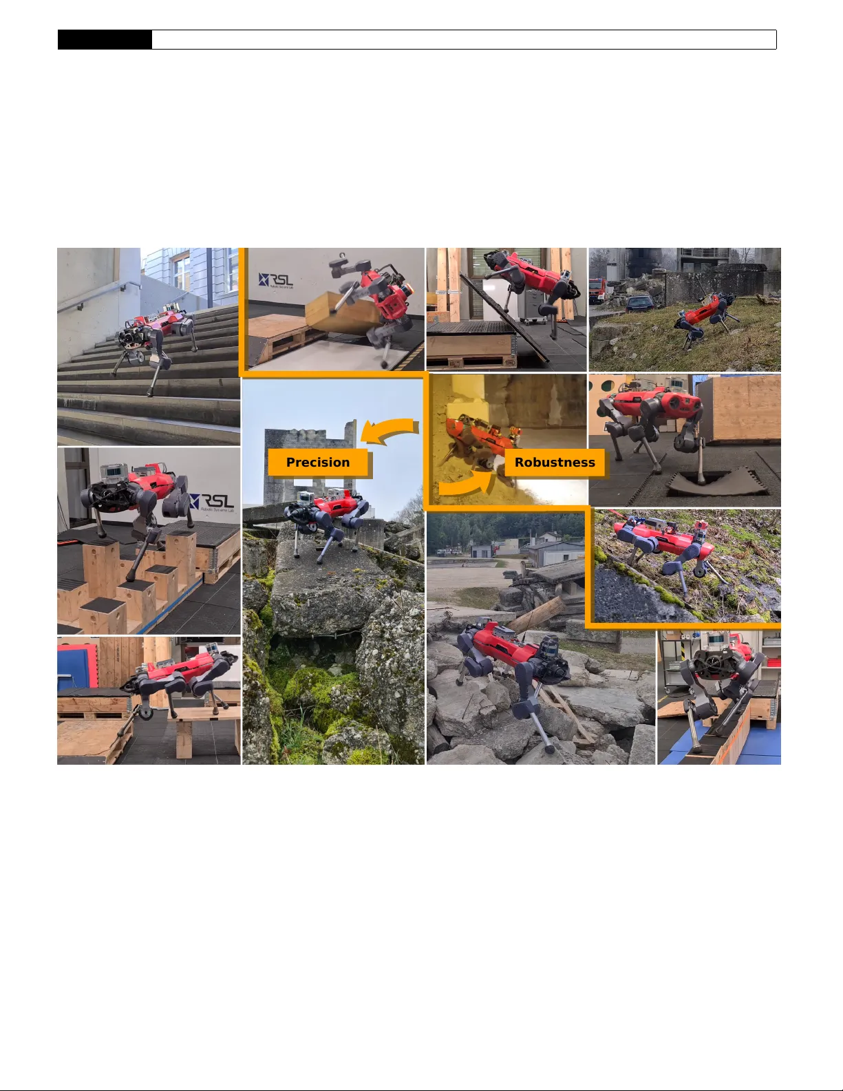
Research Ar ticle ETH Zurich 1 DTC: Deep T rac king Contr ol F A B I A N J E N E LT E N , 1 ∗ J U N Z H E H E , 1 F A R B O D F A R S H I D I A N , 2 A N D M A R C O H U T T E R 1 1 Robotic Systems Lab , ETH Zurich, 8092 Zur ich, Switzerland. 2 Currently at Boston Dynamics AI Institute, 145 Broadw ay , Cambridge MA, USA ∗ Corresponding author : f abian.jenelten@ethz.ch This is the accepted version of Science Robotics V ol. 9, Issue 86, eadh5401 (2024) DOI: 0.1126/scirobotics.adh5401 Legged locomotion is a complex contr ol pr oblem that requir es both accuracy and r obustness to cope with r eal- world challenges. Legged systems ha ve traditionally been contr olled using trajectory optimization with in verse dynamics. Such hierarchical model-based methods ar e appealing due to intuitiv e cost function tuning, accurate planning, generalization, and most importantly , the insightful understanding gained from mor e than one decade of extensive research. Howev er , model mismatch and violation of assumptions are common sources of faulty operation. Simulation-based r einfor cement learning, on the other hand, results in locomotion policies with unprecedented r obustness and r ecovery skills. Y et, all learning algorithms struggle with sparse rewards emerging from envir onments where valid footholds ar e rare, such as gaps or stepping stones. In this work, we propose a hybrid control architectur e that combines the advantages of both worlds to simultaneously achieve greater rob ustness, f oot-placement accuracy , and terrain generalization. Our approach utilizes a model-based planner to roll out a r eference motion during training . A deep neural network policy is trained in simulation, aiming to track the optimized footholds. W e ev aluate the accuracy of our locomotion pipeline on sparse terrains, where pure data-dri ven methods are pr one to fail. Furthermore, we demonstrate superior r obustness in the presence of slippery or deformable gr ound when compared to model-based counterparts. Finally , we show that our pr oposed tracking controller generalizes across different trajectory optimization methods not seen during training. In conclusion, our work unites the predicti ve capabilities and optimality guarantees of online planning with the inherent r obustness attrib uted to offline learning. INTRODUCTION Trajectory optimization ( TO ) is a commonly deployed instance of op- timal control for designing motions of legged systems and has a long history of successful applications in rough en vironments since the early 2010s [ 1 , 2 ]. These methods require a model of the robot’ s kinematics and dynamics during runtime, along with a parametrization of the ter - rain. Until recently , most approaches have used simple models such as single rigid body [ 3 ] or in verted pendulum dynamics [ 4 , 5 ], or hav e ignored the dynamic ef fects altogether [ 6 ]. Research has shifted to- wards more complex formulations, including centroidal [ 7 ] or full-body dynamics [ 8 ]. The resulting trajectories are tracked by a whole-body control ( WBC ) module, which operates at the control frequency and utilizes full-body dynamics [ 9 ]. Despite the div ersity and agility of the resulting motions, there remains a considerable g ap between simulation and reality due to unrealistic assumptions. Most problematic assump- tions include perfect state estimation, occlusion-free vision, kno wn contact states, zero foot-slip, and perfect realization of the planned motions. Sophisticated hand-engineered state machines are required to detect and respond to various special cases not accounted for in the modeling process. Ne vertheless, highly dynamic jumping maneuv ers performed by Boston Dynamics’ bipedal robot Atlas demonstrate the potential power of T O. Reinforcement learning ( RL ) has emerged as a powerful tool in recent years for synthesizing robust le gged locomotion. Unlike model- based control, RL does not rely on explicit models. Instead, beha viors are learned, most often in simulation, through random interactions of agents with the en vironment. The result is a closed-loop control policy , typically represented by a deep neural network, that maps ra w observations to actions. Handcrafted state-machines become obsolete because all relev ant corner cases are eventually visited during training. End-to-end policies, trained from user commands to joint tar get posi- tions, hav e been deployed successfully on quadrupedal robots such as ANYmal [ 10 , 11 ]. More advanced teacher -student structures have sub- stantially improv ed the rob ustness, enabling legged robots to overcome obstacles through touch [ 12 ] and perception [ 13 ]. Although locomotion across gaps and stepping stones is theoretically possible, good e xplo- ration strategies are required to learn from the emerging sparse reward signals. So far , these terrains could only be handled by specialized policies, which intentionally overfit to one particular scenario [ 14 ] or a selection of similar terrain types [ 15 – 18 ]. Despite promising results, distilling a unifying locomotion policy may be dif ficult and has only been shown with limited success [ 19 ]. Some of the shortcomings that appear in RL can be mitigated using optimization-based methods. While the problem of sparse gra- dients still exists, two important advantages can be exploited: First, cost-function and constraint gradients can be computed with a small Research Ar ticle ETH Zurich 2 Precision Robustness Fig. 1. Robust and precise locomotion in various indoor and outdoor envir onments. The marriage of model-free and model-based control allows legged robots to be deployed in en vironments where steppable contact surfaces are sparse (bottom left) and en vironmental uncertainties are high (top right). Research Ar ticle ETH Zurich 3 number of samples. Second, poor local optima can be avoided by pre- computing footholds [ 5 , 8 ], pre-segmenting the terrain into steppable areas [ 7 , 20 ], or by smoothing out the entire gradient landscape [ 21 ]. Another advantage of TO is its ability to plan actions ahead and pre- dict future interactions with the environment. If model assumptions are generic enough, this allows for great generalization across di verse terrain geometries [ 7 , 21 ]. The sparse gradient problem has been addressed extensiv ely in the learning community . A notable line of research has focused on learning a specific task while imitating expert behavior . The expert provides a direct demonstration for solving the task [ 22 , 23 ], or is used to impose a style while discov ering the task [ 24 – 26 ]. These approaches require collecting expert data, commonly done of fline, either through re-targeted motion capture data [ 24 – 26 ] or a TO technique [ 22 , 23 ]. The rew ard function can now be formulated to be dense, meaning that agents can collect non-trivial re wards e ven if they do not initially solve the task. Nonetheless, the goal is not to preserve the expert’ s accuracy but rather to lower the sample and reward complexity by leveraging existing kno wledge. T o further decrease the gap between the e xpert and the policy per - formance, we speculate that the latter should have insight into the expert’ s intentions. This requires online generation of expert data, which can be con veniently achie ved using any model-based controller . Unfortunately , rolling out trajectories is often orders of magnitude more expensi ve than a complete learning iteration. T o circumvent this problem, one possible alternati ve is to approximate the expert with a generativ e model, for instance, by sampling footholds from a uniform distribution [ 15 , 16 ], or from a neural network [ 17 , 27 , 28 ]. Howe ver , for the former group, it might be challenging to capture the distribution of an actual model-based controller, while the latter group still does not solve the e xploration problem itself. In this work, we propose to guide exploration through the solution of TO . As such data will be available both on- and offline, we refer to it as “reference” and not expert motion. W e utilize a hierarchical structure introduced in deep loco [ 28 ], where a high-le vel planner proposes footholds at a lo wer rate, and a lo w-lev el controller follows the footholds at a higher rate. Instead of using a neural network to generate the foothold plan, we leverage TO . Moreover , we do not only use the target footholds as an indicator for a rough high-lev el direction but as a demonstration of optimal foot placement. The idea of combining model-based and model-free approaches is not new in the literature. For instance, supervised [ 29 ] and unsuper- vised [ 30 , 31 ] learning has been used to warm-start nonlinear solv ers. RL has been used to imitate [ 22 , 23 ] or correct [ 32 ] motions obtained by solving TO problems. Conv ersely , model-based methods have been used to check the feasibility of learned high-lev el commands [ 27 ] or to track learned acceleration profiles [ 33 ]. Compared to [ 32 ], we do not learn correctiv e joint torques around an existing WBC , b ut in- stead, learn the mapping from reference signals to joint positions in an end-to-end fashion. T o generate the reference data, we rely on an effi cient TO method called terrain-aw are motion generation for legged systems ( T AMOLS ) [ 21 ]. It optimizes over footholds and base pose simultane- ously , thereby enabling the robot to operate at its kinematic limits. W e let the policy observe only a small subset of the solution, namely planar footholds, desired joint positions, and the contact schedule. W e found that these observ ations are more robust under the common pitfalls of model-based control, while still providing enough information to solve the locomotion task. In addition, we limit computational costs arising from solving the optimization problems by utilizing a v ariable update rate. During deployment, the optimizer runs at the fastest possible rate to account for model uncertainties and external disturbances. Our approach incorporates elements introduced in [ 14 ], such as time-based rew ards and position-based goal tracking. Howev er , we rew ard desired foothold positions at planned touch-down instead of rew arding a desired base pose at an arbitrarily chosen time. Finally , we use an asymmetric actor-critic structure similar to [ 22 ], where we provide pri vileged ground truth information to the v alue function and noisified measurements to the network policy . W e trained more than 4000 robots in parallel for two weeks on challenging ground covering a surface area of more than 76000 m 2 . Throughout the entire training process, we generated and learned from about 23 years of optimized trajectories. The combination of offline training and online re-planing results in accurate, agile, and robust locomotion. As showcased in Fig. 1 and movie 1, with our hybrid control pipeline, ANYmal [ 34 ] can skillfully traverse parkours with high precision, and confidently overcome uncertain en vironments with high robustness. Without the need for an y post-training, the tracking policy can be deployed zero-shot with different TO methods at dif ferent update rates. Moreover , movie 2 demonstrates successful deployment in search-and-rescue scenarios, which demand both accurate foot place- ment and robust recovery skills. The contributions of our work are therefore twofold: Firstly , we enable the deployment of model-based planners in rough and uncertain real-world environments. Secondly , we create a single unifying locomotion policy that generalizes beyond the limitations imposed by state-of-the-art RL methods. RESUL TS In order to ev aluate the effectiv eness of our proposed pipeline, hereby referred to as Deep Tracking Control ( DTC ), we compared it with four different approaches: two model-based controllers, T AMOLS [ 21 ] and a nonlinear model predicti ve control ( MPC ) method presented in [ 7 ], and two data-dri ven methods, as introduced in [ 13 ] and [ 11 ]. W e refer to those as baseline-to-1 ( T AMOLS ), baseline-to-2 ( MPC ), baseline-rl- 1 (teacher/student policy), and baseline-rl-2 ( RL policy), respecti vely . These baselines mark the state-of-the-art in MPC and RL prior to this work and they ha ve been tested and deployed under various conditions. If not noted differently , all experiments were conducted in the real world. Evaluation of Robustness W e conducted three experiments to e valuate the robustness of our hybrid control pipeline. The intent is to demonstrate surviv al skills on slippery ground, and recov ery reflexes when visual data is not consistent with proprioception or is absent altogether . W e rebuilt harsh en vironments that are likely to be encountered on sites of natural disasters, where debris might further break do wn when stepped onto, and construction sites, where oil patches create slippery surfaces. In the first experiment, we placed a rectangular cover plate with an area of 0.78 × 1.19 m 2 on top of a box with the same length and width, and height 0.37 m (Fig. 2 A). The cov er plate was shifted to the front, half of the box’ s length. ANYmal was then steered over the cov er plate, which pitched down as soon as its center of mass passed beyond the edge of the box. Facing only forward and backward, the plate’ s mov ement was not detected through the depth cameras, and could only be perceiv ed through proprioceptiv e sensors. Despite the error between map and odometry reaching up to 0.4 m , the robot managed to successfully balance itself. This experiment was repeated three times with consistent outcomes. In our second experiment (Fig. 2 B) we created an obstacle park- our with challenging physical properties. A large wooden box with a slopped front face was placed next to a wet and slippery whiteboard. W e increased the dif ficulty by placing a soft foam box in front, and a rolling transport cart on top of the wooden box. The robot was com- manded to walk o ver the objects with random reference v elocities for Research Ar ticle ETH Zurich 4 B slippery, r olling, and defor mable objects A moving plane C walking blind upstairs Fig. 2. Evaluation of rob ustness. (A) ANYmal walks along a loose co ver plate that e ventually pitches forward (left to right, top to bottom). The third ro w shows ANYmal’ s perception of the surroundings during the transition and reco very phase. (B) The snapshots are taken at critical time instances when walking on slippery ground, just before complete recov ery . (C) ANYmal climbs upstairs with disabled perception (top to bottom). The collision of the right-front end-effector with the stair tread triggers a swing reflex, visualized in orange. Research Ar ticle ETH Zurich 5 approximately 45 seconds, after which the objects were redistrib uted to their original locations to account for any potential displacement. This experiment was repeated fi ve times. Despite not being trained on mov able or deforming obstacles, the robot demonstrated its recov ery skills in all fiv e trials without any falls. The tracking policy was trained with perceptiv e feedback, mean- ing that the policy and the motion planner had partial or complete insight into the local geometrical landscape. Nevertheless, the loco- motion policy was still capable of overcoming many obstacles com- pletely blind. T o simulate a scenario with damaged depth sensors, we let ANYmal blindly walk over a stair with two treads, each 0.18 m high and 0.29 m wide (Fig. 2 C). The e xperiment was repeated three times up and down, with an increasing heading v elocity selected from {± 0.5, ± 0.75, ± 1.0 } m/ s . In some cases, a stair tread was higher than the swing motion of a foot. Thanks to a learned swing reflex, the stair set could be successfully cleared in all trials. W e note that the same stair set was passed by a blindfolded version of baseline-rl- 1 [ 13 ], which was trained in a complex teacher/student environment. In contrast, our method relies on an asymmetric actor/critics structure, achieving a similar le vel of robustness. Accompanying video clips can be found in the supplementary movie S1. Evaluation of Accuracy W e demonstrate the precision of foothold tracking by de vising a com- plex motion that requires the robot to perform a turn-in-place maneuver on a small surface area of 0.94 × 0.44 m 2 . The robot was commanded to walk up a slope onto a narrow table, then to execute a complete 360 deg turn, and finally to descend onto a pallet. Some snapshots of the experiment are provided in Fig. 3 A, whereas the full video is contained in movie S2. T o e valuate the quality of the foothold tracking, we collected data while ANYmal walked on flat ground. Each experiment lasted for approximately 20 s and was repeated with eight dif ferent heading ve- locities selected from {± 1.0, ± 0.8, ± 0.6, ± 0.4 } m/ s . W e measured the tracking error as the smallest horizontal distance between a foot and its associated foothold during a stance phase. As sho wn in Fig. 3 B, the footholds could be tracked with very high precision of 2.3 cm and standard deviation 0.48 cm when av eraged over the broad spectrum of heading velocity commands. Deployment with MPC The maximum height that DTC in combination with T AMOLS can reliably ov ercome is about 0.40 m . The policy might hesitate to climb up taller objects due to the risk of potential knee joint collisions with the en vironment. This limitation is inherent to the chosen TO method, which only considers simplified kinematic constraints. W e, therefore, deployed DTC with the planner of baseline-to-2, which takes into account the full kinematics of the system. T o allow for zero-shot generalization, we implemented the same trotting gait as e xperienced during training. With this enhanced setup, ANYMal could climb up a box of height of 0.48 m . This is 50 % higher than what baseline-rl-1 could climb up, and 380 % more than what w as reported for baseline-rl- 2. The box climbing experiment was successfully repeated fi ve times. The results are sho wn in movie S2, and for one selected trial in Fig. 3 D. Furthermore, we measured the tracking error on flat ground. Despite the wider stance configuration of baseline-to-2, the error was found to be only 0.03 m on a verage (Fig. 3 C). The abov e two results seem to be surprising at first glance but are easy to explain when considering the observation space and the training en vironment. Although the base-pose trajectory is considerably more detailed for baseline-to-2 due to frequency-loop shaping and increased system complexity , the foothold patterns are nev ertheless quite similar . Thus, good generalization is facilitated by the specific choice of observations, which hides the optimized base pose from the policy . Some terrains within the training environment can be seen as a combination of gaps and box es, where each box is surrounded by a gap. During training, T AMOLS placed the footholds suf ficiently far aw ay from the box to avoid stepping into the gap. This allowed the policy to learn climbing maneuvers without knee joint collisions. Baseline-to-2, being aware of the spatial coordinates of the knees, naturally produces a similar foothold pattern, ev en in the absence of the gap. Benchmark Against Model-Based Contr ol TO was proven to be effectiv e in solving complex locomotion tasks in simulation, such as the parkour shown in Fig. 4 A. This parkour has been successfully trav ersed by ANYmal using baseline-to-1 and baseline-to-2, while it w as found to be non-tra versable for baseline-rl-1 and baseline-rl-2 [ 7 ]. W ith our proposed approach, ANYmal could cross the same obstacle park our in simulation back and forth at a speed of 1 m/s , which was 20 % faster than baseline-to-1. The corresponding video clip can be found in movie S3. Model-based controllers react sensiti vely to violation of model as- sumptions, which hinders applications in real-world scenarios, where, for instance, uncertainties in friction coefficients, contact states, and visual perception may be lar ge. This issue is ex emplified in Fig. 4 B, where baseline-to-1 was used to guide ANYmal ov er a flat floor with an in visible gap. When the right front foot stepped onto the trap, the planned and e xecuted motions de viated from each other . This triggered a sequence of heuristic recov ery strategies. For large mismatches, ho w- ev er , such scripted reflex es were not ef fectiv e, and resulted in failure. DTC uses the same high-le vel planner but incorporates learned recov- ery and reflex skills. This allowed the robot to successfully navigate through the trap. The robustness is rooted in the ability to ignore both perception and reference motion while relying only on proprioception. Such behavior was learned in simulation by experiencing simulated map drift. The experiment was repeated fi ve times with baseline-to-1, fiv e times with baseline-to-2, and five times with our method, con- sistently leading to similar results. The video clips corresponding to the above experiments can be found in movie S3. The movie is fur- ther enriched with a comparison of baseline-to-2 against DTC on soft materials, which impose very similar challenges. Benchmark Against RL Contr ol Although RL policies are kno wn for their robustness, they may struggle in en vironments with limited interaction points. W e demonstrate typical failure cases in two experiments utilizing baseline-rl-1. In the first experiment (Fig. 5 A), ANYmal was tasked to cross a small gap of 0.1 m with a reference heading velocity of 0.2 m/s . The model-free controller did not a void the gap, and thus could not reach the other side of the platform. In the second experiment, we connected two elev ated boxes with a 1.0 m -long beam of height 0.2 m (Fig. 5 B). The robot was commanded to walk from the left to the right box but failed to make use of the beam. In comparison, our hybrid policy achieved a 100 % success rate for the same gap size o ver ten repetitions. T o further demonstrate the locomotion skills of DTC , we made the experiments more challenging. W e replaced the small gap with four larger gaps, each 0.6 m wide and ev enly distrib uted along the path (Fig. 5 C). Similarly , we increased the length of the beam to a total of 1.8 m (Fig. 5 D). Despite the increased difficulty , our approach maintained a 100 % success rate across four repetitions of each experiment. V ideo clips of those experiments can be found in movie S4. By using a specialized polic y , ANYmal crossed a 0.6 m wide gap within a pre-mapped en vironment [ 14 ]. Most notably , our locomotion controller , not being specialized nor fine-tuned for this terrain type, Research Ar ticle ETH Zurich 6 -1 -0.8 -0.6 -0.4 -0.2 0 0.2 0.4 0.6 0.8 1 0 0.02 0.04 0.06 0.08 0.1 LF RF LH RH -1 -0.8 -0.6 -0.4 -0.2 0 0.2 0.4 0.6 0.8 1 0 0.02 0.04 0.06 0.08 0.1 LF RF LH RH A artistic motion B foothold tracking er r or C foothold tracking er r or with baseline-to -2 D Deployment with baseline-to -2 Fig. 3. Evaluation of tracking performance. (A) ANYmal climbs up a narrow table, turns, and descends back down to a box. The second image in the second ro w shows the robot’ s perception of the en vironment. (B) Euclidean norm of the planar foothold error , averaged o ver 20 s of operation using a constant heading velocity . The solid/dashed curves represent the av erage/maximum tracking errors. (C) Same representation as in (B), but the data w as collected with baseline-to-2. (D) DTC deployed with baseline-to-2, enabling ANYMal to climb up a box of 0.48 m . Research Ar ticle ETH Zurich 7 A obstacle park our simulation (ours) B collapsing fl oor (baseline-to -1) C collapsing fl oor (ours) Fig. 4. Benchmarking against model-based control. (A) DTC successfully trav erses an obstacle parkour (left to right) in simulation with a heading velocity of 1 m/s . (B) Baseline-to-1 falls after stepping into a g ap hidden from the perception (left to right). (C) ANYmal successfully ov ercomes a trapped floor using our hybrid control architecture (left to right). crossed a sequence of four gaps with the same width, whilst, relying on online generated maps only . The limitations of baseline-rl-1 were pre viously demonstrated [ 7 ] on the obstacle parkour of Fig. 4 A, sho wing its inability to cross the stepping stones. W e sho wcase the generality of our proposed control framew ork by conducting three experiments on stepping stones in the real world, each with an increased level of difficulty . The first experiment (Fig. 6 A) required ANYmal tra versing a field of equally sized stepping stones, providing a contact surface of 0.2 × 0.2 m 2 each. The robot passed the 2.0 m long field 10 times. Despite the varying heading velocity commands, the robot accurately hit the correct stepping stones as indicated by the solution of the TO . For the second experiment (Fig. 6 B), we increased the height of two randomly selected stones. The parkour was successfully crossed four out of four times. In the final experiment (Fig. 6 C), we distributed three ele vated platforms a , b , and c , connected by loose wooden blocks of sizes 0.31 × 0.2 × 0.2 m 3 and 0.51 × 0.2 × 0.2 m 3 . This en vironment posed considerable challenges as the blocks may move and flip over when stepped on. Follo wing the path a → b → a → b → c → a , the robot missed only one stepping stone, which, ho we ver , did not lead to failure. V ideo clips of the stepping stones experiments are pro vided in movie S5. Simulation-Based Ablation Study During training, we computed a solution to the TO problem after vari- able time interv als, but mainly after each foot touch-do wn. Although such a throttled rate greatly reduced computational costs, it also leads to poor reactiv e behavior in the presence of quickly changing external disturbances, dynamic obstacles, or map occlusion. Moreover , the optimizer was updated using privile ged observations, whereas, in real- ity , the optimizer is subject to ele vation map drift, wrongly estimated friction coef ficients, and unpredicted external forces. T o compensate for such modeling errors, we deploy the optimizer in MPC -fashion. W e in vestigated the locomotion performance as a function of the optimizer update rate. Using the experimental setup outlined in the supplemen- tary methods (section “Experimental Setup for Evaluation of Optimizer Rate”), we collected a total of six days of data in simulation. A robot was deemed “successful” if it could walk from the center to the border of its assigned terrain patch, “failed” if its torso made contact with the en vironment within its patch, and “stuck” otherwise. W e report success and failure rates in Fig. 7 A. Accordingly , when increasing the update rate from 1 Hz to 50 Hz , the failure rate dropped by 7.11 % whereas the success rate increased by 4.25 % . In the second set of experiments, we compared our approach against baseline-rl-2 as well as against the same policy trained within our train- ing environment. W e refer to the emer ging policy as baseline-rl-3. More details regarding the experimental setup can be found in the supplementary methods (section “Experimental Setup for Performance Evaluation”). As depicted in Fig. 7 B i, our approach exhibited a substantially higher success rate than baseline-rl-2. By learning on the same terrains, baseline-rl-3 could catch up b ut still did not match our performance in terms of success rate. The difference mainly orig- inates from the fact that the retrained baseline still failed to solve sparse-structured terrains. T o highlight this observation, we e valuated the performance on four terrain types with sparse (“stepping stones”, “beams”, “gaps”, and “pallets”), and on four types with dense stepping locations (“stairs”, “pit”, “rough slope”, and “rings”). On all consid- ered terrain types, our approach outperformed baseline-rl-2 by a huge margin (Fig. 7 B ii), thereby demonstrating that learned locomotion generally does not extrapolate well to unseen scenarios. W e performed equally well as baseline-rl-3 on dense terrains, but scored notably higher on sparse-structured terrains. This result suggests that the pro- posed approach itself was effecti ve and that fav orable locomotion skills were not encouraged by the specific training en vironment. In an additional experiment, we in vestigated the effects of erroneous predictions of the high-lev el planner on locomotion performance. W e did so by adding a drift value to the ele vation map, sampled uniformly Research Ar ticle ETH Zurich 8 A small gap (baseline-rl-1) B short beam (baseline-rl-1) D long beam (ours) C sequence of lar ge gaps (ours) Fig. 5. Benchmarking against reinfor cement learning . (A) Baseline-rl-1 attempts to cross a small gap. ANYmal initially manages to recover from miss-stepping with its front le gs but subsequently gets stuck as its hind le gs fall inside the gap. (B) Using baseline-rl-1, the robot stumbles along a narro w beam. (C) With DTC , the robot can pass four consecuti ve large gaps (left to right) without getting stuck or f alling. (D) ANYmal is crossing a long beam using the proposed control framew ork. Research Ar ticle ETH Zurich 9 A stepping stones B stepping stones with height di ff er ence C loose stepping stones a b c Fig. 6. Evaluation of the locomotion perf ormance on stepping stones. (A) ANYmal reliably crosses a field of flat stepping stones (left to right). (B) The robot crosses stepping stones of varying heights (left to right). The two tall blocks are highlighted in blue. (C) ANYmal navigates through a field of loosely connected stepping stones, following the path a → b → a → b → c → a . Research Ar ticle ETH Zurich 10 ours baseline-rl-2 baseline-rl-3 0 20 40 60 80 100 success failed stuck A optimizer fr equency D training curves with/withoutout desir ed joint positions fr om IK B sim perfor mance (all ter rains) 0 20 40 60 80 1.5 2 2.5 3 with without 0 20 40 60 80 3.5 4 4.5 5 with without C tracking perfor mance and success rate as a function of map drif t (all ter rains) stairs pit rough rings stepping stones pallets beams gaps 0 20 40 60 80 100 ours baseline-rl-2 baseline-rl-3 10 0 10 1 0 20 40 60 success failed stuck ii ii 0 0.2 0.4 0 50 100 success failed stuck 0 0.2 0.4 0 50 100 success failed stuck 0 0.1 0.2 0.3 0.4 0.02 0.04 0.06 0.08 flat rough iii ii i i i Fig. 7. Simulation results and ablation studies . (A) Success and failure rates of DTC , recorded for dif ferent update rates of the optimizer . The upper limit of 50 Hz is imposed by the polic y frequency . (B) Comparison against baseline policies. (i) Evaluation on all 120 terrains. (ii) Evaluation on terrains where valid footholds are dense (white background) and sparse (gray background). (C) Influence of elev ation map drift on the locomotion performance, quantified by tracking error (i) , success rate on rough (ii) , and on flat ground (ii) . (D) A verage terrain le vel (i) and av erage foothold rew ard (ii) scored during training. Research Ar ticle ETH Zurich 11 from the interval ∈ ( 0, 0.5 ) m . Contrary to training, the motion was optimized over the perturbed height map. Other changes to the ex- perimental setup are described in the supplementary methods (section “Experimental Setup for Performance Evaluation under Drift”). As visualized in Fig. 7 C, we collected tracking error , success, and failure rates with simulated drift on flat and rough ground. The tracking error grew mostly linearly with the drift v alue (Fig. 7 C i). On rough terrains, the success rate remained constant for drift v alues smaller than 0.1 m , and decreased linearly for larger values (Fig. 7 C ii). On the other hand, success and failure rates were not af fected by drift on flat ground (Fig. 7 C iii). W e found that pro viding joint positions computed for the upcoming touch-down event greatly improv ed con vergence time and foothold tracking performance. This signal encodes the foothold location in joint space, thus, providing a useful hint for foothold tracking. It also simplifies the learning process, as the network is no longer required to implicitly learn the in verse kinematics ( IK ). Evidence for our claims is giv en in Fig. 7 D, showing two rele vant learning curves. Tracking accuracy is represented by the foothold rewards, whereas technical skills are quantified using the average terrain le vel [ 11 ]. Both scores are substantially higher if the footholds could be observed in both task and joint space. DISCUSSION This work demonstrates the potential of a h ybrid locomotion pipeline that combines accurate foot placement and dynamic agility of state-of- the-art TO with the inherent robustness and reflex beha viors of nov el RL control strate gies. Our approach enables legged robots to overcome complex en vironments that either method alone would struggle with. As such terrains are commonly found in construction sites, mines, and collapsed buildings, our work could help advance the deployment of autonomous legged machines in the fields of construction, maintenance, and search-and-rescue. W e hav e rigorously ev aluated the performance in extensiv e real- world experiments ov er the course of about half a year . W e included gaps, stepping stones, narrow beams, and tall boxes in our tests, and demonstrated that our method outperformed the RL baseline controller on ev ery single terrain. Next, we e valuated the rob ustness on slippery and soft ground, each time outperforming two model-based controllers. Furthermore, we have shown that the emerging policy can track the motion of two different planners utilizing the same trotting gait. This was possible because the observed footholds seem to be mostly in variant under the choice of the optimizer . Howe ver , certain obstacles may encourage the deployed planner to produce footprint patterns that otherwise do not emerge during training. In this case, we would expect a degraded tracking performance. In addition to our main contribution, we hav e demonstrated sev eral other notable results. First, our policy , which was trained e xclusiv ely with visual perception, is still able to generalize to blind locomotion. Second, A simple multilayer perceptron ( MLP ) trained with an asym- metric actor/critics setup achiev es similar robust behaviors as much more complex teacher/student trainings [ 12 , 13 ]. Third, Our locomo- tion policy can handle a lot of noise and drift in the visual data without relying on complicated gaited networks, which might be difficult to tune and train [ 13 ]. Contrary to our expectations, the proposed training environment was found to not be more sample efficient than similar unifying RL approaches [ 11 , 13 ]. The large number of epochs required for con- ver gence suggests that foothold accuracy is something intrinsically complicated to learn. In this work, we emphasized that TO and RL share complementary properties and that no single best method exists to address the open challenges in legged locomotion. The proposed control architecture lev erages this observation by combining the planning capabilities of the former and the robustness properties of the latter . It does, by no means, constitute a universal recipe to integrate the two approaches in an optimal way for a generic problem. Moreover , one could even extend the discussion with self- and unsupervised learning, indirect optimal control, dynamic programming, and stochastic optimal control. Nev ertheless, our results may moti vate future research to incorporate the aspect of planning into the concept RL. W e see sev eral promising avenues for future research. Many suc- cessful data-driv en controllers hav e the ability to alter the stride dura- tion of the trotting gait. W e expect a further increase in surviv al rate and technical skills if the network policy could suggest an arbitrary contact schedule to the motion optimizer . Moreov er , a truly hybrid method, in which the policy can directly modify the cost function of the planner, may be able to generate more diversified motions. Our results indicate that IK is difficult to learn. T o increase the sample efficienc y and improve generalization across different platforms, a more sophisticated network structure could exploit prior knowledge of analytical IK . Another potential research direction may focus on lev eraging the benefits of sampling trajectories from an of fline buffer . This could substantially reduce the training time and allo w for the substitution of T AMOLS with a more accurate TO method, or even expert data gathered from real animals. MA TERIALS AND METHODS Motivation T o motivate the specific architectural design, we first identify the strengths and weaknesses of the two most commonly used control paradigms in legged locomotion. TO amounts to open-loop control, which produces suboptimal so- lutions in the presence of stochasticity , modeling errors, and small prediction windo ws. Unfortunately , these methods also introduce many assumptions, mostly to reduce computation time or achiev e fa vorable numerical properties. F or instance, the feet are almost alw ays pre- selected interaction points to prevent complex collision constraints, contact and actuator dynamics are usually omitted or smoothed out to circumvent stif f optimization problems, and the contact schedule is often pre-specified to av oid the combinatorial problem imposed by the switched system dynamics. Despite a large set of strong assumptions, real-time capable planners are not always truly real-time. The reference trajectories are updated around 5 Hz [ 31 ] to 100 Hz [ 7 ] and realized between 400 Hz to 1000 Hz. In other words, these methods do not plan fast enough to catch up with the errors they are making. While struc- tural [ 2 ] or environmental [ 7 , 20 ] decomposition may further contribute to the ov erall suboptimality , the y were found useful for extracting good local solutions on sparse terrains. Because the concept of planning is not restricted to the tuning domain, model-based approaches tend to generalize well across dif ferent terrain geometries [ 7 , 21 ]. Moreover , since numerical solvers perform v ery cheap and sparse operations on the elev ation map, the map resolution can be arbitrarily small, facilitat- ing accurate foothold planning. RL , on the other hand, leads to policies that represent global closed- loop control strategies. Deep neural networks are large capacity models, and as such, can represent locomotion policies without introducing any assumption about the terrain or the system (except from being Marko- vian). They exhibit good interpolation in-between visited states but do not extrapolate well to unseen en vironments. Despite their large size, the inference time is usually relativ ely small. The integration of an actu- ator model has been demonstrated to improve sim-to-real-transfer [ 10 ], while the stochasticity in the system dynamics and training en viron- ment can effecti vely be utilized to synthesize robust beha viors [ 12 , 13 ]. Research Ar ticle ETH Zurich 12 Contrary to TO , the elev ation map is typically down-sampled [ 11 , 13 ] to av oid immense memory consumption during training. In summary , TO might be better suited if good generalization and high accuracy are required, whereas RL is the preferred method if robustness is of concern or onboard computational power is limited. As locomotion combines challenges from both of these fields, we formulate the goal of this work as follo ws: RL shall be used to train a low-le vel tracking controller that provides markedly more rob ustness than classical in verse dynamics. The accuracy and planning capabilities of model-based TO shall be leveraged on a low lev el to synthesize a unifying locomotion strategy that supports diverse and generalizing motions. Reference Motions Designing a TO problem for control always inv olves a compromise, that trades off ph ysical accuracy and generalization against good nu- merical conditioning, low computation time, conv exity , smoothness, av ailability of deriv ativ es, and the necessity of a high-quality initial guess. In our work, we generate the trajectories using T AMOLS [ 21 ]. Unlike other similar methods, it does not require terrain segmenta- tion nor pre-computation of footholds, and its solutions are robust under varying initial guesses. The system dynamics and kinematics are simplified, allowing for f ast updates. During deployment, we also compare against baseline-to-2, which builds up on more comple x kin- odynamics. Due to the increased computation time and in particular the computationally demanding map-processing pipeline, this method is not well-suited to be used directly within the learning process (the training time would be expected to be about eight times lar ger). W e added three crucial features to T AMOLS : First, we enable par- allelization on CPU, which allo ws multiple optimization problems to be solved simultaneously . Second, we created a python interface using pybind11 [ 35 ], enabling it to run in a python-based en vironment. Finally , we assume that the measured contact state always matches the desired contact state. This renders the TO independent of contact estimation, which typically is the most fragile module in a model-based controller . The optimizer requires a discretized 2.5 d representation of its en- vironment, a so-called elev ation map, as input. W e extract the map directly from the simulator by sampling the height across a fixed grid. For both training and deployment, we use a fixed trotting gait with a stride duration of 0.93 s and swing phase of 0.465 s , and set the resolution of the grid map to 0.04 × 0.04 m 2 . Overview of the T raining En vironment The locomotion policy π ( a | o ) is a stochastic distribution of actions a ∈ A that are conditioned on observations o ∈ O , parametrized by an MLP . The action space comprises target joint positions that are tracked using a PD controller , following the approach in [ 10 ] and related works [ 12 – 14 ]. Giv en the state s ∈ S , we extract the solution at the next time step x ′ ( s ) ∈ X ⊆ S from the optimizer , which includes four footholds p ∗ i = 0,. ..,3 , joint positions q ∗ at touch-do wn time, and the base trajectory ev aluated at the next time step. The base trajectory consists of of base pose b ∗ ( ∆ t ) , twist ˙ b ∗ ( ∆ t ) , and linear and angular acceleration ¨ b ∗ ( ∆ t ) . More details can be found in Fig. 8 A. W e then sample an action from the polic y . It is used to forward simulate the system dynamics, yielding a new state s ′ ∈ S , as illustrated in Fig. 8 B. T o define a scalar reward r ( s , s ′ , x ′ , a ) , we use a monotonically decreasing function of the error between the optimized and measured states, that is r ∝ x ′ ( s ) ⊖ x ( s ′ ) . The minus operator ⊖ is defined on the set X , the vector x ′ ( s ) is the optimized state, and x ( s ′ ) is the state of the simulator after extracting it on the corresponding subset. The policy network can also be understood as a learned model reference adaptiv e controller with the optimizer being the reference model. In this work, we use an asymmetrical actor/critic method for train- ing. The value function approximation V ( o , ˜ o ) uses privile ged ˜ o ∈ ˜ O as well as policy observ ations o . Observation Space The value function is trained on policy observ ations and privileged ob- servations, while the polic y network is trained on the former only [ 22 ]. All observations are gi ven in the robot-centric base frame. The defini- tion of the observ ation vector is gi ven below , whereas noise distrib u- tions and dimensionalities of the observ ation vectors can be found in the supplementary methods and T able 2 . P olicy Observations The policy observ ations comprise propriocepti ve measurements such as base twist, gra vity vector , joint positions, and joint velocities. The history only includes previous actions [ 11 ]. Additional observations are extracted from the model-based planner , including planar coordinates of foothold positions ( x y coordinates), desired joint positions at touch- down time, desired contact state, and time left in the current phase. The latter two are per-le g quantities that fully describe the gait pattern. Footholds only contain planner coordinates since the height can be extracted from the height scan. The height scan, which is an additional part of the observ ation space, enables the network to anticipate a collision-free swing le g trajectory . In contrast to similar works, we do not construct a sparse ele vation map around the base [ 11 , 27 ] or the feet [ 13 ]. Instead, we sample along a line connecting the current foot position with the desired foothold (Fig. 8 A). This approach has several adv antages: First, the samples can be denser by only scanning terrain patches that are most rele vant for the swing leg. Second, it pre vents the netw ork from e xtracting other information from the map, which is typically exposed to most uncertainty (for instance, occlusion, reflection, odometry drift, discretization error , etc.). Third, it allows us to con veniently model elevation map drift as a per-foot quantity , which means that each leg can ha ve its o wn drift value. W e use analytical IK to compute the desired joint positions. As the motion optimizer may not provide a swing trajectory , as is the case for T AMOLS , we completely skip the swing phase. This means that the IK is computed with the desired base pose and the measured foot position for a stance leg, and the tar get foothold for a swing leg. It is worth noting that we do not provide the base pose reference as observation. This was found to reduce sensitivity to mapping errors and to render the policy independent of the utilized planner . Finally , to allow the network to infer the desired walking direction, we add the reference twist (before optimization) to the observation space. Privileged Obser vations The privileged observations contain the optimized base pose, base twist, and base linear and angular acceleration, e xtracted one time step ahead. In addition, the critics can observe signals confined to the simulator, such as the external base wrench, external foot forces, the measured contact forces, friction coefficients, and ele vation map drift. Rewar d Functions The total reward is computed as a weighted combination of sev eral individual components, which can be categorized as follo ws: “tracking” of reference motions, encouraging “consistent” behavior , and other “regularization” terms necessary for successful sim-to-real transfer . The rew ard functions are explained below whereas weights and parameters are reported in T able 3 . Research Ar ticle ETH Zurich 13 A B C D a b f e i j c g k l d h Fig. 8. Overview of the training method and deployment strategy . (A) The optimized solution provides footholds p ∗ i , desired base pose b ∗ , twist ˙ b ∗ , and acceleration ¨ b ∗ (extracted one polic y step ∆ t ahead), as well as desired joint positions q ∗ . Additionally , a height scan h is sampled between the foot position p i and the corresponding foothold. (B) Training en vironment: The optimizer runs in parallel to the simulation. At each leg touch-do wn, a new solution x ′ is generated. The policy π driv es the system response s ′ tow ard the optimized solution x ′ ( s ) , which is encouraged using the re ward function r . Actor observations are perturbed with the noise vector n , while critics and the TO receiv e ground truth data. (C) Deployment: Giv en the optimized footholds, the network computes target joint positions that are track ed using a PD control la w . The state estimator (state) returns the estimated robot state, which is fed back into the policy and the optimizer . (D) The list of terrain types includes a) stairs, b) combinations of slopes and gaps, c) p yramids, d) slopped rough terrain, e) stepping stones, f) objects with randomized poses, g) boxes with tilted surfaces, h) rings, i) pits, j) beams, k) ho vering objects with randomized poses, and l) pallets. Research Ar ticle ETH Zurich 14 Base Pose T racking T o achie ve tracking of the reference base pose trajectory , we use r Bn = e − σ Bn ·| | b ∗ ( t + ∆ t ) ( n ) ⊖ b ( t ) ( n ) || 2 , (1) where n = { 0, 1, 2 } is the deriv ative order , b ( t ) is the measured base pose, b ∗ ( t + ∆ t ) is the desired base pose sampled from the reference trajectory one policy step ∆ t ahead, and ⊖ denotes the quaternion difference for base orientation and the vector dif ference otherwise. W e refer to the above reward function as a “soft” tracking task because large v alues can be scored ev en if the tracking error does not perfectly vanish. T o further analyze the reward function, we decompose the base trajectory into three segments. The “head” starts at time zero, the “tail” stops at the prediction horizon, and the “middle” connects these two segments with each other . A logarithmic rew ard function would prioritize the tracking of the trajectory head, while a linear penalty would focus on making progress along the whole trajectory at once. Contrary , the exponential shape of the reward function splits the track- ing task into several steps. During the initial epochs, the tracking error of the trajectory middle and tail will likely be relati vely large, and thus, do not contribute notably to the re ward gradient. As a result, the network will minimize the tracking error of the trajectory head. Once its effect on the gradient diminishes, the errors corresponding to the trajectory middle will dominate the gradient landscape. In the final training stages, tracking is mostly improv ed around the trajectory tail. Foothold T racking W e choose a logarithmic function r pi = − ln ( || p ∗ i − p i || 2 + ϵ ) , (2) to learn foothold tracking, where p i is the current foot position of leg i ∈ { 0, . . . , 3 } , p ∗ i is the corresponding desired foothold, and 0 < ϵ ≪ 1 is small number ensuring the function is well defined. The abov e reward function may be termed a “hard” tracking task, as the maximum value can only be scored if the error reaches zero. As the tracking improv es, the gradients will become larger , resulting in ev en tighter tracking tow ard the later training stages. A dense reward structure typically encourages a stance foot to be dragged along the ground to further minimize the tracking error . T o prevent such drag motions from emerging, the above reward is giv en for each foot at most once during one complete gait cycle: more specifically , if and only if the leg is intended to be in contact and the norm of the contact force indicates a contact, that is if || f i || > 1 , then the agent receiv es the rew ard. Consistency In RL for legged locomotion, hesitating to mo ve o ver challenging ter - rains is a commonly observed phenomenon that pre vents informati ve samples from being gathered and thus impedes the agent’ s performance. This behavior can be explained by insuf ficient exploration: The major- ity of agents f ail to solv e a task while a small number of agents achie ve higher av erage rewards by refusing to act. T o overcome this local opti- mum, we propose to encourage consistency by re warding actions that are intended by previous actions. In our case, we measure consistency as the similarity between two consecutive motion optimizations. If the solutions are similar, the agent is considered to be “consistent”. W e measure similarity as the Euclidean distance between two adjacent solutions and write r c = ∑ δ t j + t 0 ∈ ( T a ∩ T b ) − δ t | | b ∗ a ( δ t j + t 0, a ) ⊖ b ∗ b ( δ t j + t 0, b ) | | − w p || p ∗ a − p ∗ b || . (3) Here, p ∗ t with t = { a , b } is a vector of stacked footholds, w p > 0 is a relativ e weight, δ t = 0.01 s is the discretization time of the base trajectory , and t 0 is the time elapsed since the solution was retrie ved. The index a refers to the most recent solution, while b refers to the previous solution. It is important to note that the two solution vectors x a and x b , from which we extract the base and footholds, are only defined on their respective time intervals given by the optimization horizon τ h , i.e, t a ∈ T a = [ 0, τ h , a ] and t b ∈ T b = [ 0, τ h , b ] . Regularization T o ensure that the robot walks smoothly , we employ two different penalty terms enforcing complementary constraints. The first term, r r 1 = − ∑ i | v T i f i | , discourages foot-scuffing and end-eff ector col- lisions by penalizing power measured at the feet. The second term, r r 2 = − ∑ i ( ˙ q T i τ i ) 2 , penalizes joint power to prevent arbitrary mo- tions, especially during the swing phase. Other regularization terms are stated in the supplementary methods (section “Implementation Details”). T raining En vironment T o train the locomotion policy , we employ a custom version of Proximal Policy Optimization ( PPO )[ 36 ] and a training en vironment that is mostly identical to that introduced in[ 11 ]. It is explained in more detail in the supplementary methods (section “T raining Details”) and T able 1 . Simulation and back-propagation are performed on GPU, while the optimization problems are solved on CPU. T ermination W e use a simple termination condition where an episode is terminated if the base of the robot makes contact with the terrain. Domain Randomization W e inject noise into all observations except for those designated as privile ged. At each policy step, a noise vector n is sampled from a uniform distribution and added to the observation vector , with the only exceptions of the desired joint positions and the height scan. For the elevation map, we add noise before extracting the height scan. The noise is sampled from an approximate Laplace distribution where large values are less common than small ones. W e perturb the height scan with a constant offset, which is sampled from another approximate Laplace distribution for each foot separately . Both per- turbations discourage the network to rely extensi vely on perceptive feedback and help to generalize to various perceptiv e uncertainties caused by odometry drift, occlusion, and soft ground. All robots are artificially pushed by adding a twist of fset to the measured twist at regular time instances. Friction coefficients are ran- domized per leg once at initialization time. T o render the motion rob ust against disturbances, we perturb the base with an external wrench and the feet with external forces. The latter slightly stiff ens up the swing motion but impro ves tracking performance in the presence of unmod- eled joint frictions and link inertia. The reference twist is resampled in constant time intervals and then held constant. The solutions for the TO problems are obtained using ground truth data, which include the true friction coefficients, the true external base wrench, and noise-free height map. In the presence of simulated noise, drift, and external disturbances, the policy network is therefore trained to reconstruct a base trajectory that the optimizer would produce given the ground truth data. Howe ver , there is a risk that the network learns to remov e the drift from the height scan by analyzing the desired joint positions. During hardware deployment, such a reconstruction will fail because the optimizer is subject to the same height drift. T o mitigate this issue, we introduce noise to the desired joint position observations, sampled from a uniform distrib ution with boundaries proportional to the drift value. Research Ar ticle ETH Zurich 15 T errain Curriculum W e use a terrain curriculum as introduced in [ 11 ]. Before the training process, terrain patches of varying types and dif ficulties are generated, and each agent is assigned a terrain patch. As an agent acquires more skills and can navigate the current terrain, its le vel is upgraded, which means it will be re-spawned on the same terrain type, but with a harder difficulty . W e have observed that the variety of terrains encountered during training influences the sim-to-real transfer . W e thus hav e in- cluded a total of 12 different terrain types with configurable parameters (Fig. 8 D), leading to a total of 120 distinguishable terrain patches. The terrain types classify different locomotion behaviors, s.a. climbing (“stairs”, “pits”, “box es”, “pyramids”), reflexing (“rough”, “rings”, “flying objects”), and w alking with lar ge steps (“gaps”, “pallets”, “step- ping stones”, “beams”, “objects with randomized poses”). Our terrain curriculum consists of 10 lev els, where one of the configurable param- eters is modulated to increase or decrease its dif ficulty . This results in a total of 1200 terrain patches, each with a size of 8 × 8 m 2 , summing up to a total area of 76800 m 2 , which is approximately the size of 14 football fields or 10 soccer fields. T raining Solving the TO problems at the policy frequenc y during training was found to prov oke poor local optima. In such a case, the optimizer adapts the solution after each policy step: If the agent is not able to follow the reference trajectory , the optimizer will adapt to the ne w state s.t. the tracking problem becomes feasible again. This means that the agent can exhibit “lazy” behavior and still collect some rewards. W e prevent such a local optimum by updating the optimizer only at a leg touch-down (after 0.465 seconds). This also greatly reduces learning time because computational costs are reduced by a factor of 23 . After a robot fell (on average, once e very 18 seconds), was pushed (after 10 seconds) or its twist commands changed (three times per episode), the optimized trajectories are no longer v alid. T o guarantee that the locomotion polic y generalizes across different update rates, we additionally recompute the solution in all those scenarios. W e trained the policy with a massiv e parallelization of 64 2 = 4096 robots, for a total of 90000 epochs. Each epoch consisted of 45 learning iterations where each iteration covered a duration of 0.02 seconds. Considering the variable update rate explained pre viously , this resulted in a total of 8295 days (or 23 years) of optimized trajectories. The policy can be deplo yed after about one day of training ( 6000 epochs), reaches 90 % of its peak performance after three days ( 20000 epochs), and is fully con ver ged after two weeks ( 90000 epochs). In comparison, the baseline-rl-1 polic y was trained for 4000 epochs with 1000 parallelized robots over 5 consecutiv e days. Each epoch lasted for 5 seconds, resulting in a throughput of 46 simulated seconds per second. Our polic y was trained for 14 days, with each epoch lasting for 0.9 seconds, leading to a throughput of 27 simulated seconds per second. Thus, despite generating 1.6 years of desired motions per day , our approach has only a 1.7 times lower throughput than the baseline. Deployment W e deploy the polic y at a frequency of 50 Hz without any fine-tuning. The motion optimizer runs at the largest possible rate in a separate thread. For T AMOLS with a trotting gait, this is around 400 Hz and for baseline-to-2 around 100 Hz (both are faster than the policy frequenc y). At each step, the policy queries the most recent solution from the thread pool and extracts it ∆ t = 0.02 s ahead of the most recent time index. For our experiments, we used three different types of ANYmal robots [ 34 ], two version C and one version D, for which we trained different policies. ANYmal C is by default equipped with four Intel RealSense D435 depth cameras whereas ANYmal D has eight depth cameras of the same type. For the second V ersion C, the depth cameras were replaced with two identical Robosense Bpearl dome LiDAR sensors. For the outdoor experiments, we mostly used this robot, as the Bpearls tend to be more robust against lighting conditions. Motion optimization and the forward propagation of the network policy are done on a single Intel core-i7 8850H machine. Elev ation mapping [ 37 ] runs on a dedicated onboard Nvidia Jetson. REFERENCES 1. J. Z. Kolter, M. P . Rodgers, A. Y . Ng, A control architecture for quadruped locomotion over rough terrain, 2008 IEEE International Confer ence on Robotics and Automation , 811–818 (2008). 2. M. Kalakrishnan, J. Buchli, P . Pastor, M. Mistry, S. Schaal, F ast, robust quadruped locomotion over challenging terrain, 2010 IEEE International Confer ence on Robotics and Automation , 2665–2670 (2010). 3. A. W . Winkler, C. D . Bellicoso, M. Hutter, J . Buchli, Gait and trajector y optimization for legged systems through phase-based end-effector parameterization, IEEE Robotics and Automation Letters 1560–1567 (2018). 4. C. Mastalli, I. Havoutis , M. Focchi, D . G. Caldwell, C. Semini, Mo- tion planning for quadrupedal locomotion: Coupled planning, terrain mapping, and whole-body control, IEEE T ransactions on Robotics 1635– 1648 (2020). 5. F . Jenelten, T . Miki, A. E. Vijay an, M. Bjelonic, M. Hutter , P erceptive lo- comotion in rough terrain – online foothold optimization, IEEE Robotics and Automation Letters 5370–5376 (2020). 6. P . F ankhauser, M. Bjelonic, C. Dario Bellicoso, T . Miki, M. Hutter, Robust rough-terrain locomotion with a quadrupedal robot, 2018 IEEE International Conference on Robotics and Automation (ICRA) , 5761– 5768 (2018). 7. R. Grandia, F . Jenelten, S. Y ang, F . F arshidian, M. Hutter , Perceptiv e locomotion through nonlinear model-predictive control, IEEE T ransac- tions on Robotics 1–20 (2023). 8. C. Mastalli, W . Merkt, G. Xin, J . Shim, M. Mistr y , I. Havoutis , S. Vijay aku- mar , Agile maneuvers in legged robots: a predictive control approach (2022). 9. C. D . Bellicoso, F . Jenelten, C. Gehring, M. Hutter, Dynamic locomotion through online nonlinear motion optimization f or quadr upedal robots, IEEE Robotics and Automation Letters 2261–2268 (2018). 10. J. Hw angbo , J. Lee , A. Dosovitskiy , D . Bellicoso, V . Tsounis, V . Koltun, M. Hutter , Lear ning agile and dynamic motor skills f or legged robots, Science Robotics p. eaau5872 (2019). 11. N. Rudin, D . Hoeller, P . Reist, M. Hutter , Learning to walk in minutes using massively parallel deep reinf orcement lear ning, 5th Annual Con- fer ence on Robot Learning (2021). 12. J. Lee, J. Hwangbo , L. Wellhausen, V . Koltun, M. Hutter , Lear ning quadrupedal locomotion over challenging terrain, Science Robotics p . eabc5986 (2020). 13. T . Miki, J. Lee, J . Hwangbo , L. Wellhausen, V . K oltun, M. Hutter , Lear n- ing robust perceptive locomotion for quadr upedal robots in the wild, Science Robotics p. eabk2822 (2022). 14. N. Rudin, D . Hoeller , M. Bjelonic, M. Hutter , Advanced skills b y learning locomotion and local navigation end-to-end, 2022 IEEE/RSJ Interna- tional Confer ence on Intelligent Robots and Systems (IROS) , 2497–2503 (2022). 15. Z. Xie, H. Y . Ling, N. H. Kim, M. v an de P anne, Allsteps: Curr iculum- driven learning of stepping stone skills, Computer Graphics F orum 39 (2020). 16. H. Duan, A. Malik, J. Dao , A. Saxena, K. Green, J. Siekmann, A. F ern, J. Hurst, Sim-to-real learning of f ootstep-constrained bipedal dynamic walking, 2022 International Conference on Robotics and Automation (ICRA) , 10428–10434 (2022). 17. W . Y u, D . J ain, A. Escontrela, A. Iscen, P . Xu, E. Coumans, S. Ha, J. T an, T . Zhang, Visual-locomotion: Learning to walk on comple x terrains with vision, Pr oceedings of the 5th Conference on Robot Learning , A. F aust, D . Hsu, G. Neumann, eds., 1291–1302 (PMLR, 2022). 18. A. Agarwal, A. Kumar , J . Malik, D . Pathak, Legged locomotion in Research Ar ticle ETH Zurich 16 challenging terrains using egocentric vision, 6th Annual Confer ence on Robot Learning (2022). 19. K. Caluwaerts, A. Iscen, J. C. K ew , W . Y u, T . Zhang, D . F reeman, K.-H. Lee, L. Lee, S . Saliceti, V . Zhuang, N. Batchelor , S. Bohez, F . Casar ini, J. E. Chen, O . Cor tes, E. Coumans, A. Dostmohamed, G. Dulac- Arnold, A. Escontrela, E. Fre y , R. Hafner , D . Jain, B. Jy enis, Y . K uang, E. Lee, L. Luu, O . Nachum, K. Oslund, J. P owell, D . Reyes , F . Romano , F . Sadeghi, R. Sloat, B. T abanpour , D . Zheng, M. Neuner t, R. Hadsell, N. Heess, F . Nori, J. Seto , C. Par ada, V . Sindhwani, V . V anhouck e, J. T an, Barkour: Benchmarking animal-level agility with quadruped robots (2023). 20. R. J. Griffin, G. Wiedebach, S. McCrory , S. Ber trand, I. Lee, J. Pratt, Footstep planning for autonomous walking over rough terrain, 2019 IEEE-RAS 19th International Conference on Humanoid Robots (Hu- manoids) , 9–16 (2019). 21. F . Jenelten, R. Gr andia, F . F arshidian, M. Hutter , T amols: T errain-aware motion optimization for legged systems, IEEE T ransactions on Robotics 3395–3413 (2022). 22. P . Brakel, S . Bohez, L. Hasenclever , N. Heess, K. Bousmalis, Learning coordinated terrain-adaptive locomotion by imitating a centroidal dy- namics planner , 2022 IEEE/RSJ International Confer ence on Intelligent Robots and Systems (IR OS) , 10335–10342 (2022). 23. M. Bogdanovic, M. Khadiv , L. Righetti, Model-free reinforcement learn- ing for robust locomotion using demonstrations from trajectory opti- mization, F rontiers in Robotics and AI 9 (2022). 24. X. B. P eng, P . Abbeel, S. Levine, M. van de Panne , Deepmimic: Example-guided deep reinforcement learning of physics-based charac- ter skills, A CM T ransactions on Graphics 37 (2018). 25. X. B. Peng, Z. Ma, P . Abbeel, S. Levine , A. Kanazawa, Amp: Adver- sarial motion priors for styliz ed physics-based character control, A CM T ransactions on Graphics 40 (2021). 26. S. Bohez, S . T unyasuvunak ool, P . Brakel, F . Sadeghi, L. Hasenclever , Y . T assa, E. P ar isotto , J . Humplik, T . Haarnoja, R. Hafner , M. Wulfmeier , M. Neunert, B. Moran, N. Siegel, A. Huber, F . Romano , N. Batchelor , F . Casar ini, J. Merel, R. Hadsell, N. Heess, Imitate and repur pose: Learning reusable robot mov ement skills from human and animal be- haviors (2022). 27. V . Tsounis, M. Alge, J. Lee, F . F arshidian, M. Hutter , Deepgait: Planning and control of quadrupedal gaits using deep reinforcement lear ning, IEEE Robotics and Automation Letters 3699–3706 (2020). 28. X. B. P eng, G. Berseth, K. Yin, M. v an de Panne , Deeploco: Dynamic locomotion skills using hierarchical deep reinforcement learning, ACM T ransactions on Graphics (Proc. SIGGRAPH 2017) 36 (2017). 29. O . Melon, M. Geisert, D . Surovik, I. Hav outis, M. F allon, Reliable trajectories for dynamic quadrupeds using analytical costs and learned initializations (2020). 30. D . Surovik, O. Melon, M. Geisert, M. F allon, I. Havoutis , Learning an expert skill-space for replanning dynamic quadr uped locomotion ov er obstacles, Pr oceedings of the 2020 Conference on Robot Learning , J. K ober , F . Ramos, C . T omlin, eds., 1509–1518 (PMLR, 2021). 31. O . Melon, R. Orsolino , D . Surovik, M. Geiser t, I. Hav outis, M. F al- lon, Receding-horizon perceptiv e trajectory optimization for dynamic legged locomotion with learned initialization, 2021 IEEE International Confer ence on Robotics and Automation (ICRA) , 9805–9811 (2021). 32. S. Gangapurwala, M. Geisert, R. Orsolino, M. F allon, I. Havoutis , Rloc: T errain-aware legged locomotion using reinforcement learning and optimal control, IEEE T ransactions on Robotics 2908–2927 (2022). 33. Z. Xie, X. Da, B. Babich, A. Garg, M. v . de P anne, Glide: Generaliz- able quadrupedal locomotion in diverse environments with a centroidal model, Algorithmic F oundations of Robotics XV , S. M. LaV alle, J. M. O’Kane, M. Otte, D . Sadigh, P . T okekar , eds., 523–539 (Springer Inter- national Publishing, Cham, 2023). 34. M. Hutter , C. Gehring, D . Jud, A. Lauber, C . D . Bellicoso, V . Tsounis, J. Hwangbo , K. Bodie, P . F ankhauser , M. Bloesch, R. Diethelm, S . Bach- mann, A. Melzer , M. Hoepflinger, Hutter2016 - a highly mobile and dynamic quadrupedal robot, 2016 IEEE/RSJ International Confer ence on Intelligent Robots and Systems (IROS) , 38–44 (2016). 35. W . J akob , J . Rhinelander , D . Moldov an, p ybind11 – seamless operability between c++11 and p ython (2017). Https://github .com/pybind/p ybind11. 36. J. Schulman, F . Wolski, P . Dhariwal, A. Radford, O . Klimov , Proximal policy optimization algorithms, CoRR abs/1707.06347 (2017). 37. T . Miki, L. Wellhausen, R. Grandia, F . Jenelten, T . Homberger , M. Hutter , Elev ation mapping for locomotion and navigation using gpu (2022). 38. F . Jenelten, J. He, F . Farshidian, M. Hutter, Evaluation of tracking performance and robustness f or a hybrid locomotion controller , https: //doi.org/10.5061/dryad.b5mkkwhkq . A CKNO WLEDGMENTS Funding: This project has receiv ed funding from the European Re- search Council (ERC) under the European Union’ s Horizon 2020 re- search and innov ation programme grant agreement No 852044. This research was supported by the Swiss National Science F oundation (SNSF) as part of project No 188596, and by the Swiss National Science Foundation through the National Centre of Competence in Re- search Robotics (NCCR Robotics). A uthor Contribution: F .J. formu- lated the main ideas, trained and tested the policy using baseline-to-1, and conducted most of the experiments. J.H. interfaced baseline-to-2 with the tracking policy and conducted the box-climbing experiments. F .F . contributed to the Theory and improved some of the original ideas. All authors helped to write, improve, and refine the paper . Competing interests: The authors declare that they ha ve no competing interests. Data and materials a vailability: All (other) data needed to ev aluate the conclusions in the paper are present in the paper or the Supplemen- tary Materials. Data-sets and code to generate all our figures are made publicly av ailable [ 38 ]. Research Ar ticle ETH Zurich 17 SUPPLEMENT AR Y METHODS Nomenclature ( · ) i index for le g i ∈ { 0, . . . , 3 } τ h prediction horizon b ∗ ( t ) optimized base pose trajectory ˙ b ∗ ( t ) optimized base twist trajectory ¨ b ∗ ( t ) optimized base acceleration trajectory q ∗ optimized joint positions obtained from IK p ∗ i optimized foothold p t vector of stacked footholds, computed at time t p i measured foot position f i measured contact force v i measured foot velocity q i measured joint positions τ i measured joint torques s state of the robot x ′ ( s ) solution of optimization problem one time-step ahead, initialized with state s x ( s ′ ) state s ′ extracted on subset of the optimizer o policy observ ations ˜ o privileged observ ations a actions T raining Details W e use a simulation time step of 5 ms and a policy time step of 20 ms. The elev ation map noise is sampled from a Laplace distribution, which is approximated by two uniform distributions. W e first sam- ple the boundaries of the uniform distrib ution h n , m a x ∼ U ( 0, 0.2 ) m , and then sample the noise from h n ∼ U ( − h n , m a x , h n , m a x ) . Sim- ilar holds for the height drift: W e first sample the boundaries h d , m a x ∼ U ( 0, 0.2 ) m and then sample five drift values h d 0 , . . . , h d 4 ∼ U ( − h d , m a x , h d , m a x ) , where h d 0 is constant for the entire map and h d 1 . . . . , h d 4 is sampled for each foot individually . The total drift h d is obtained by summing up the map-drift and the per-foot drift. Elev ation map noise and drift are re-sampled after a constant time interval of 8 s . The noise vector added to the desired joint positions depends on the height drift, and is sampled from the uniform distribution q n ∼ 2 · U ( − h d , h d ) . W e push the robots after 10 s by adding a twist offset to the mea- sured twist sampled from ∆ ˙ b ∼ U ( − 1, 1 ) [ m / s ] . Friction coefficients are randomized per le g and sampled from µ ∼ U ( 0.1, 1.2 ) . For each episode, we sample an external base wrench τ B ∼ U ( − 15, 15 ) and a external foot force f ee ∼ U ( − 2, 2 ) N . The reference twist is re-sampled from a uniform distribution three times per episode. A third of the robots has zero lateral velocity whereas the heading velocity is sampled from v x ∼ U ( − 1, 1 ) m/s . Another third has zero heading velocity and its lateral velocity is sampled from v y ∼ U ( − 0.8, 0.8 ) m/s . The last third has mixed heading and lateral velocities sampled from their respectiv e distri- butions. F or all three cases, the yaw velocity is sampled from v ψ ∼ U ( − 0.8, 0.8 ) rad /s . The PPO hyperparameters used for the training are stated in T able 1 . All policies were trained with a seed of 1 . Implementation Details T o parameterize the policy (or actor) network, a Gaussian distrib ution is used, where the mean is generated by an MLP parametrized by θ . The standard de viation is added independently of the observ ations as an additional layer in the network. Specifically , the policy can be written as π ( a | o ) ∼ N ( µ θ ( o ) , σ θ ) , where µ θ ( o ) represents the mean and σ θ the standard deviation. The value function (or critics) is generated by another MLP as V ( o , ˜ o ) ∼ N ( µ ϕ ( o , ˜ o ) , 0 ) , which is parametrized parameter type number batch size 45 · 4096 = 184320 mini batch size 4 · 4096 = 16384 number of epochs 5 clip range 0.2 entropy coef ficient 0.0035 discount factor 0.99 GAE discount factor 0.95 desired KL-div ergence 0.01 learning rate adaptiv e T able 1. PPO hyperparameters . The value 4096 is the number of parallelized en vironments. All policies were trained with the same parameters. by ϕ . For both MLP’ s we use three hidden layers with each having 512 neurons. Observations are normalized using running means and running standard deviation. Policy and privileged observations can be found in T able 2 , and relativ e weights of the re ward functions are giv en in T able 3 . The implementation of most of the re ward functions are gi ven in the main text. In addition to those, we penalize the action rate r a = −| | a t − a t − 1 || 2 and joint acceleration r ¨ q = − || ¨ q || 2 , with a t , a t − 1 being the current and previous actions, and ¨ q the measured joint accelerations. Experimental Setup for Evaluation of Optimizer Rate The e xperimental setup mostly coincided with the training en vironment as detailed in the supplementary methods (section “Training Details”), with four minor diff erences: The terrain curriculum was disabled, and for each terrain type, we selected the most difficult one. A push or a velocity change did not trigger a new solution to be computed. The optimizer was not informed about the true values for friction coefficients and e xternal base wrenches. Instead, nominal values were used. All robots were walking in heading direction with a reference velocity sampled uniformly from the interval 0.8 . . . 0.95 m /s . The robots were pushed after 5 s with a disturbance twist sampled from the interval ∆ ˙ b ∼ U ( − 2, 2 ) m/s , which is twice as much as experienced during training. W e did not add external foot forces, noise, or map drift. For each optimizer rate in { 1, 2, 2.5, 3.3, 5, 10, 20, 50 } Hz , the success and failure rates were av eraged over 8 different e xperiments conducted with varying seeds selected from the interval { 2, . . . , 9 } . Each experiment w as conducted with 4096 robots, distributed across 120 terrains, lasting for one episode ( = 20 s ). Experimental Setup for Performance Evaluation Baseline-rl-3 used the same observations and policy structure as baseline-rl-2. But it was trained within the same en vironment as ours using a comparable number of epochs. For the e valuation on all terrains, we used the training en vironment as detailed in the supplementary methods (section “Training Details”), with the follo wing simplifications: The terrain curriculum w as disabled, and for each terrain type, we selected the most difficult one. All robots were walking in heading direction with a reference v elocity sampled uniformly from the interval 0.8 . . . 0.95 m /s . W e did not add external foot forces, noise, or map drift. The friction coefficients between feet and ground were set to 1 . In addition, for the ev aluation on specific terrains, we did not push the robots, and we did not re-sample Research Ar ticle ETH Zurich 18 type observations dim noise policy base twist 6 gravity v ector 3 ± 0.05 joint positions 12 ± 0.01 joint velocities 12 ± 1.5 previous actions 12 0 planar footholds 8 ± 0.05 desired joint positions 12 Laplace desired contact state 4 time left in phase 4 reference twist 3 height scan 40 Laplace privile ged desired base position 3 desired base quaternion 4 desired base twist 12 consistency re ward 1 external base wrench 6 external foot force 12 friction coefficients 4 height drift 4 T able 2. Policy and privileged obser vations . The column “noise” contains the upper and lo wer values of the uniform distrib ution, with units identical to that one of the observ ations. Entries marked with “Laplace” indicate the noise distrib ution is sampled from an approxi- mate Laplace distribution as e xplained in the supplementary methods (section “T raining Details”). A missing value indicates that the noise lev el is zero. rew ard type rew ard name weight parameter tracking base position 1 σ = 1200 base rotation 1 σ = 90 base linear velocity 1 σ = 10 base angular velocity 1 σ = 1 base linear acceleration 1 σ = 0.05 base angular acceleration 1 σ = 0.005 footholds 6 ϵ = 10 − 5 consistent behavior consistenc y 20 regularization foot power − 0.02 joint power − 0.025 action rate − 0.02 joint acceleration − 10 − 6 T able 3. Reward functions . the reference velocities. This setup relaxes the locomotion task on topologically hard terrains such as stepping stones, that otherwise might not be traversable. Results were averaged over eight different seeds. Experimental Setup for Performance Evaluation under Drift The e xperimental setup mostly coincided with the training en vironment as detailed in the supplementary methods (section “Training Details”), with the following differences: The terrain curriculum was disabled, and for each terrain type, we selected the most difficult one. All robots were walking in heading direction with a reference v elocity sampled uniformly from the interval 0.8 . . . 0.95 m /s . W e did not add external foot forces or noise. The friction coefficients between feet and ground were set to 1 . W e did not push the robots and we did not re-sample the reference velocities. In addition, for the flat ground experiment, we replaced all terrain types with a single horizontal plane. Each experiment was repeated 21 times with a linearly increasing drift value selected from { 0.0, 0.025, . . . , 0.5 } m . Results were averaged over eight different seeds.