2.75D: Boosting learning by representing 3D Medical imaging to 2D features for small data
In medical-data driven learning, 3D convolutional neural networks (CNNs) have started to show superior performance to 2D CNNs in numerous deep learning tasks, proving the added value of 3D spatial information in feature representation. However, the d…
Authors: Xin Wang, Ruisheng Su, Weiyi Xie
2.75D: Boosting Learning by R epresenting 3D Medical Imaging to 2D Features f or Small Data Xin W ang a ,1 , Ruisheng Su b ,1 , W eiyi Xie c , W enjin W ang d , Ritse Mann a , Jungong Han e and T ao T an a , ∗ a Department of Radiology, the Netherlands Cancer Institute, Plesmanlaan 121, Amsterdam, 1066 CX, The Net herlands b Erasmus Medical Center Rotter dam, Doctor Molewaterplein 40, Rotter dam, 3015 CD, The Nether lands c Radboud Univer sity Medical Center , Geert Gr ooteplein Zuid 10, Nijmeg en, 6525 GA, The Netherlands d Biomedical Engineer ing Depar tment of Souther n Univer sity of Science and T echnology, Xueyuan Blvd 1088, Shenzhen, 518055, China e Computer Science, F ellow of IAPR, Aber ystwyth Univer sity, UK A R T I C L E I N F O Keyw ords : Medical imaging Spiral sampling 2.75D Deep lear ning MRI CT Luna cancer Breast cancer Prostate Cancer A B S T R A C T In medical-data driven lear ning, 3D con volutional neural networks (CNNs) hav e star ted to show superior performance to 2D CNNs in numerous deep learning tasks, proving the added value of 3D spatial information in f eature representation. How ever , t he difficulty in collecting more training samples to conv erg e, more comput ational resources and longer ex ecution time make this approach less applied. Also, applying transf er learning on 3D CNN is challenging due to a lack of publicly av ailable pre-trained 3D models. To t ackle these issues, we proposed a novel 2D strategical representation of volume tric data, namely 2.75D. In this work, the spatial information of 3D images is captured in a single 2D view by a spiral-spinning technique. As a result, 2D CNN networks can also be used to learn volumetric information. Besides, we can fully leverag e pre-trained 2D CNNs for downstream vision problems. W e also explore a multi-view 2.75D strategy , 2.75D 3 channels (2.75D × 3), to boost the advantage of 2.75D. W e ev aluated the proposed methods on three public datasets with different modalities or organs (Lung CT, Breast MRI, and Prostate MRI), against their 2D, 2.5D, and 3D counterpar ts in classification tasks. Results show that the proposed methods significantly outper form other counterpar ts when all methods were trained from scratch on the lung dataset. Such per formance gain is more pronounced with transf er lear ning or in the case of limited training data. Our methods also achie ved comparable per formance on other datasets. In addition, our methods achieved a substantial reduction in time consumption of training and inference compared with the 2.5D or 3D method. 1. Introduction 1.1. Clinical Back gr ound Cancer is the second leading cause of death worldwide [ 1 ], including lung, breast, and pros tate cancers, which are the most widespread cancers in t he developed w orld. Earl y detection based on radiog raphic screening programs, such as X -ra y , Computed T omography (CT), and Magnetic Reso- nance Imaging (MRI), has t he potential to improv e the prog- nosis and reduce mor tality f or patients [ 1 ]. The effectiveness of cancer treatments heavil y depends on the phase at which the cancer is diagnosed. For example, the five-y ear survival rate f or a localized stage of non-small cell lung cancer is much higher t han t hat for the distant stage [ 2 ]. Howe ver , the implementation of widespread cancer screening programs in the w orld will likely lead to a substantial amount of medical images, while the wor kload and the shor t age of screening radiologists are severe. In addition, due to the large size of medical images, finding earl y subtle abnor malities is a time- consuming and thus error-prone t ask for radiologists. ∗ Corresponding author taotanjs@gmail.com (T. Tan) OR CI D (s): 1 X. W ang and R. Su hav e equal contributions 1.2. Relat ed Wor k Benefited from the recent advances in Con volutional Neural Netw orks (CNNs) in various computer vision chal- lenges [ 3 , 4 , 5 ], man y algor ithms for automatic cancer di- agnosis on medical images hav e been proposed to help to impro ve radiologists’ per formance and reduce t heir work - load. Logically , increasingly amount of studies hav e been dev oted on the adoption of CNN in t he medical imaging field, where data ha ve different high-dimension natures, such as 2D images (X -ray [ 6 ], 2D ultrasound [ 7 ]) and 3D volumes (CT [ 8 ], Computed Tomographic Angiography (CT A) [ 9 ], 3D ultrasound [ 10 ], MRI [ 11 ]), 2D images+Time sequence ([ 12 , 13 ]), 3D images+Time sequence ([ 14 ]). 2D CNN is one of the most import ant netw orks in the machine learning field, whic h made im pressive achie ve- ments in the past f ew years. Since AlexN et [ 15 ] was pro- posed, the re volution of deep CNN on large-scale dat asets ( e.g . ImageN et [ 15 ], which contains 1.4 million images with 1000 classes) was tr iggered. With emphasizing the import ance of depth [ 4 ], deeper network structures emerg ed, such as GoogleNet [ 16 ] and VGG [ 4 ], which significantly impro ved the per f or mance in classification tasks. Af terward, He et al. [ 5 ] introduced skip connections in ResN et to solv e the vanishing gradients problems. While 2D CNNs go deeper and deeper, these state-of-t he-art (SOT A) CNNs ha ve also been extensiv ely explored on medical images and different tasks, such as the malignancy classification of liv er Xin Wang, Ruisheng Su et al.: Preprint submitted to Elsevier Page 1 of 13 2.75D: Bo osting Learning by Representing 3D Imaging to 2D masses [ 17 ], cancer types discr imination [ 18 ], and intracra- nial aneurysm detection [ 19 ]. Moreov er, many well-kno wn 2D CNNs pre-trained on the large ImageNet dataset are open to the public and readily accessible, which suppor ts transf er learning. It is cr itical in the context of medical images wit h small datasets and a lack of annotations, due to the cost and necessary w orkload of radiologists. Regular 2D CNN approaches are well known f or han- dling 2D image classification tasks. Howe ver , 2D CNNs are not directly applicable to 3D medical images. Based on the model input representation of 3D data, existing CNN methods can be mainly divided into three categor ies: 2D, 2.5D, and 3D. Firstly , a straightf or w ard approach is to take a representative 2D slice from t he 3D v olume as model input [ 20 ], named t he 2D method. Such a representation generally f ails to capture sufficient volumetric stereo information. V ar - ious studies hav e shown the inferior per formance of 2D CNN versus other approaches which incor porate stereo informa- tion. For e xample, Setio et al. [ 8 ] utilized multiview 2D CNN f or pulmonary nodule classification, which outper f or med single-view 2D CNN. T o best lear n high dimensional features, many SOT A 3D CNN approaches hav e been inv estigated for 3D med- ical imaging [ 21 , 22 , 23 ], whic h can extr act v olumetric f eatures from entire volumes without losing inf ormation, demonstrating promising impro vements in many computer- aided diagnosis applications. For example, Y ang et al. [ 2 4 ] trained a 3D CNN for Alzheimer’ s Disease classification. The superior ity of 3D CNN was demonstrated in their wor k by compar ing to baseline 2D CNNs. More ex amples of 3D CNN approaches in medical imaging include pulmonary nodule classification [ 25 ], brain hemor rhage classification [ 26 ], Alzheimer diagnosis [ 24 ], and breast cancer classifi- cation [ 27 ]. Howe ver , due to the limited av ailability of dat a and high comput ational resources, practice of 3D CNNs on medical images is discouraged [ 28 ]. With the success of 2D CNNs and the limitations of 3D CNNs, various studies ha v e also attempted to repre- sent 3D volumes in multiple 2D views, which is t he 2.5D method. For ex ample, Lyksborg et al. [ 29 ] used 2D CNNs on three ort hogonal 2D patches to incor porate 3D contextual inf ormation. Su et al. [ 30 ] utilized trained multiple CNN streams, each using one 2D view of t he object for 3D shape classification. Similarl y , Setio et al. [ 8 ] extracted nine differently or iented v olume slices and f ed them into separate streams of 2D CNNs for pulmonar y nodule classification. 2.5D methods generally are betw een 2D and 3D approaches and better in training efficiency comparing to 3D methods [ 8 , 31 , 32 , 33 , 34 ]. As aforementioned, 2.5D CNN requires f ew er GPU resources than 3D CNN, and incorporates richer v olumetric information of neighbor ing vo xels t han the 2D method. On t he other hand, the biggest problem from 2.5D is that the v ox els from 3D are not strategically sampled in a single 2D image while the geometry relation between vo x els is lost, which means 2.5D cannot strategicall y represent t he inf ormation needed for diagnosis from 3D. Graph represent ation may also be able to represent the relations of different regions efficientl y . For example, Zhang et al. [ 13 ] use a multiplex visibility g raph to represent 2D+times ser ies recordings. Howe v er, this method also has limitations, such as t he need to correspond to a standard (brain) atlas to extract t he graph structure. Su et al. [ 35 ] defined t he anatomical region b y atlas-based registration and then extracted high-level features from CT A. This is hard for lung, breast, or prostate imaging due to t he huge personalized variations. Is there a better 2D representation of 3D volumes other than 2.5D? To answer this, we revisit the spiral scanning techniq ue in this w ork. Spiral scanning is an existing con- cept, which has been initially proposed in signal sampling in the phy sical space of imaging. For exam ple, W ang et al. [ 36 ] adopted spiral scanning for cone-beam recons tr uction in 2007. In the same year , spiral scanning was exploited f or the sake of dynamic programming segment ation in 2D [ 37 ]. In 2014, Rana et al. [ 38 ] utilized spiral scanning to impro ve the control of atomic f orce microscope. Despite various applications of spiral scanning, it has not been e xplored f or efficient 3D to 2D representation in CNNs. Recentl y , lots of effor ts hav e been paid on aspects such as designing architectures of deep-lear ning networks, improving lear ning scheme by optimizing hyperparameters, and increasing dat a diversity by augmenting limited data. Rarel y , research has been focused on the data representation domain. Dat a repre- sentation is more than image preprocessing. Preprocessing mainly ref ers to image nor malization, noise reduction and artifact remov al, which makes follo w-up processing f ocus on clinical-related image f eatures. Those transf or mations are pixel-le vel and intensity-le v el changes. Data representation furt her transf orms t he data into a new form which might make the follo w-up processing be more comfortable. In summar y , t he significant c hallenge in 3D medical imaging is t he requirement f or high-efficiency representation of volume tr ic information, bey ond resource limit ation and fully lev eraging pre-trained CNNs. This is a key factor in the dev elopment of 3D medical imaging-based CAD sys tems in clinic practice. Current SOT A 3D approaches generally out- perform 2D or 2.5D approac hes while requiring significantl y more dat a for training, consuming more GPU resources as well as limiting the ability to use transf er lear ning. 1.3. Contributions T o this end, we proposed our 2.75D method 2 , which boosts the computational efficiency and lear ning capability of deep learning netw orks on 3D image classification tasks using the spiral scanning techniq ue. W e ha ve extended our previous Open Arxiv v ersion [ 39 ], with e xplored robust multi-view 2.75D strategy and validated on more public datasets. Our approach serves as a generic framew ork for generating a sufficient 2D present ation of a 3D volume. When sample frequency is set to a small value, the approac h can be reduced to 2D or 2.5 approaches. Meanwhile, our 2 The T ensorFlow and PyTorc h implementations of our code av ailable at https://github.com/RuishengSu/2.75D Xin Wang, Ruisheng Su et al.: Preprint submitted to Elsevier P age 2 of 13 2.75D: Bo osting Learning by Representing 3D Imaging to 2D approach r uns faster than 2.5D approaches, similar to the 2D method, while can maint ain relativ ely good per f orma nce compared to 3D me thods. By con verting 3D v olume to a sufficient 2D representation, it is beneficial to perform transf er lear ning using models trained ov er a larg e number of natural images [ 15 ], whereas pre-trained models for 3D medical images are rare. The significant per formance gain of incor porating transf er lear ning on 2.75D is demonstrated in compar ison with 3D approaches. The main contr ibutions of this paper are as follo ws: • W e proposed a 2.75D s trategy to extr act efficient 2D representations of a 3D v olume as the input to a 2D classification CNN instead of a 3D CNN. • W e ev aluated t he proposed methods on t hree public datasets wit h different modalities and different organs and demonstrated its remarkable per formance in compar ison to 2D, 2.5D, and 3D approaches. • W e explor ed the capability and advantage of 2.75D using transf er lear ning via pre-trained models from large-scale 2D image data sets that are publicly av ailable. • W e systematically inv estigated the effect of dat a size on training yield from different approaches. 2. Method In t his section, the proposed 2.75D strategies are ex- plained in detail, especiall y ho w 3D volumes are trans- f ormed into cor responding 2D represent ations. Provided a 3D v olume classification task , CNNs can be utilized to lear n textural and volume tr ic information from t he sur rounding v olume of a given candidate v ox el. T o boost the efficiency of such CNN based methods, we propose to first transf or m these 3D volumes into 2D representations using the spiral scanning techniq ue, f ollow ed by a 2D CNN classifier which can lear n volume tric inf or mation as in 3D CNNs. By repr esenting 3D v olumes in a 2D fashion, man y exis ting 2D CNNs can be adopted for solving 3D image vi- sion problems (e.g. nodule classification in chest CT, breast MRI, and prostate MRI). W e hypothesize that such a 2D representation would contain volume tric inf or mation. For enhanced featur e extraction from 3D volumes, we further explore a multi-spiral-view strategy named 2.75D 3channels (2.75D × 3). The patc h extraction process is explained in detail below . 2.1. Spir al Scanning for 2D P atc h Extraction The wor kflow of 3D to 2D transf ormation is illustrated in Fig. 1a . Given a 3D cubic volume of size 𝑑 × 𝑑 × 𝑑 , a sphere with a radius of 𝑟 = 𝑑 ∕2 is defined at the v olume center . The spiral scanning process sample v ox els from 3D coordinate space to generate a 2D image via the mov ement of a scanning line (shown in gray dotted lines). During the scanning pro- cess, the star ting point of t he scanning line is alwa ys at the v olume center, but its end-point mo ves on the sphere surface (a) 2.75D (b) 2.75D 3 channels (2.75D × 3) Fig. 1: (a) T ransfo rmation of a 3D volume to 2D representation using spiral scanning. Each dotted line in light grey color rep resents a sampled radial line originated from the sphere center to a surface p oint. 32 intensity values are on each sampled radial line, which forms one column in the transfo rmed 2D image. 123 radial lines from top to b ottom of the sphere a re ordered from left to right in the transfo rmed 2D image. (b) Three different views for multi-view spiral scanning. from the topmost point to the lowes t point at the bottom, while circling around the central axis (default parallel to the Z-axis) counter-cloc kwise. According to t he patched 64 × 64 × 64 3D cubic, the heights of resampled images are alwa ys 32. Such a mov ement on a 3D space can be decomposed into tw o rotation angles: t he azimuth (longitude) angle 𝛼 ∈ [0 , 𝜋 ] defining the mo vement v er tically and elev ation (latitude) angle 𝛽 ∈ [0 , 2 𝜋 ] descr ibing the horizont al mov ement. To make t he transf orm discrete, the spiral scanning undergoes a sampling process. First, the mov ement is captured in steps by sampling two rotation angles at a fix ed inter val. W e show t he sampled steps using a sequence of surface points (dark solid dots) along the scanning trajectory on the sphere surface (dark solid lines). Second, at each step, a fix ed number of v ox els are sampled along the scanning line in the 3D volume. All sampled vo x els are rear ranged in a 2D image sequentiall y as t he sampling process goes, where row s indicate mov ement steps, and each column is filled with vo x els sampled on the scanning line. Suppose that t he spiral line is densely distributed around the sphere, t he lengt h of t he spiral scanning orbit would be approximatel y equal to t he sum of circumf erences of a number of separate hor izontal circles. For simplicity , the number of sur f ace points is calculated based on this appro x- imation. Suppose the angle step is 𝜋 ∕ 𝑁 , t he azimut h and elev ation angles are evenl y divided into 𝑁 ( 𝛼 𝑘 = 𝑘𝜋 ∕ 𝑁 , 𝑘 = Xin Wang, Ruisheng Su et al.: Preprint submitted to Elsevier P age 3 of 13 2.75D: Bo osting Learning by Representing 3D Imaging to 2D Fig. 2: Patch examples from 2.5D and the proposed 2.75D in the LIDC-IDRI dataset. Left: nine differently oriented views of V OIs concatenated (size: 64 × (64 × 9) = 64 × 576 px); right: extracted spiral view patches of V OIs (size: 32 × 123 px); a: non-no dule examples; b: no dule examples. 0 , 1 , 2 , ..., 𝑁 ) and 2 𝑁 ( 𝛽 𝑘 = 𝑘𝜋 ∕ 𝑁 , 𝑘 = 0 , 1 , 2 , ..., 2 𝑁 ) sections, respectiv ely . The number of sample points on a hor- izontal circle at 𝛼 can be e xpressed as 2 𝜋 | sin( 𝛼 ) | ∕( 𝜋 ∕ 𝑁 ) , i.e., 2 𝑁 sin( 𝛼 ) , regardless of the sphere radius. Theref ore, the total number of sample points on the sphere sur face is appro ximately 4 𝑁 2 ∕ 𝜋 when N is large, as expressed in Eq. 1 . In t his work, we choose 𝑁 = 9 for a v olume of 64 × 64 × 64 to produce 123 sample points that equal to t he width of the resampled image (as shown in Fig. 1a ). More import antly , a 32 × 123 image is smaller than a 2D image ( 64 × 64 ). When 𝑁 = 10 , the number of sample points is 147, which will be larger than the 2D image. For a fair comparison with the 2D method and to pro ve that the superior ity of our method is due to a higher efficient informative sampling strategy rather than more sample pixels, we set t he image size to be 32 × 123 . 𝑁 ∑ 𝑘 =0 2 𝑁 | sin( 𝑘𝜋 ∕ 𝑁 ) | ≈ 2 𝑁 ∫ 𝑁 0 | sin( 𝑘𝜋 ∕ 𝑁 ) | 𝑑 𝑘 = 2 𝑁 ∫ 𝑁 0 ( 𝑁 ∕ 𝜋 ) | sin( 𝑘𝜋 ∕ 𝑁 ) | 𝑑 ( 𝑘𝜋 ∕ 𝑁 ) = 2 𝑁 2 ∕ 𝜋 ∫ 𝜋 0 | sin 𝑥 | 𝑑 𝑥 = 4 𝑁 2 ∕ 𝜋 (1) As sho wn in Fig. 1b , the spiral scanning is around the center axis, which is parallel to the Z-axis by default. Similar to the 2.5D approach, when we use the x-axis and t he y-axis, and the z-axis as t he def ault axes, respectivel y , we can extract three 2D representations. After spiral scanning, the 2D representations of the 3D v olumes are obtained, which agg regate 3D information in all directions via the spiral scanning process. Some examples of the resulted spiral view images are sho wn in Fig. 2 . These 2D patches can then be fed into neural netw orks for training and inf erence instead of 3D volumetric data. 3. Materials T o ev aluate the per formance of the proposed strategy , we compare t he per formance of four strategies (2D, 2.5D, 3D, 2.75D, and 2.75D 3 channels) on the classification task on three official dat a sets. They are from the LUNA16 nodule detection g rand challenge 3 , the PR OST A TEx challeng e 4 and Duke-Breast-Cancer -MRI 5 [ 40 ]. W e also demonstrate the effect of transfer lear ning on 2.75D. More, we ev aluate the performance of different approaches with the adjustment of training data sizes. 3.1. Datasets and Pr eprocessing 3.1.1. LUN A16 - Nodule or non-nodule classification: The LUN A16 challenge consists of two sub-tasks based on a tw o-stage nodule detection pipeline. The first is to detect nodule candidates on given CT scans, which may include f alse positives; The second task is to classify each nodule candidate into nodule or non-nodule given its sur rounding 3D volume on the CT scan. W e participated in the f alse pos- itive reduction in the nodule detection pipeline. In total, 888 CT scans are included in t he challenge data set. CT scans all 3 https://luna16.grand- challenge.org/ 4 https://prostatex.grand- challenge.org/ 5 https://doi.org/10.7937/TCIA.e3sv- re93 Xin Wang, Ruisheng Su et al.: Preprint submitted to Elsevier P age 4 of 13 2.75D: Bo osting Learning by Representing 3D Imaging to 2D (a) 2D: single view 2D CNN architecture (b) 2.5D: multi-view 2D CNN arc hitecture (c) 3D: v olume based 3D CNN architecture (d) 2.75D: spiral view based CNN architecture (e) 2.75D 3channels: multi-spiral-view based CNN architecture Fig. 3: Architectures of 2D, 2.5D, 3D, 2.75D and 2.75D 3channels (2.75D × 3) app roaches ha ve slice thickness and are less than 2.5 millimeters. In the ref erence standard, nodules were annotated by the consensus of f our radiologists in two phases. For t he false positive reduction trac k, nodule candidates wer e generated using a set of existing automated nodule detection algorithms [ 41 , 42 , 43 ]. In total, 1120 out of 1186 nodules are detected with 551,065 candidates. More information regarding t he annotation protocol and the procedure for nodule candidate generation can be found in [ 44 ]. W e f ollowed the preprocessing procedure descr ibed by Setio et al. [ 8 ]. A 50 × 50 × 50 mm volume of interest (V OI) w as extracted from each of the candidate nodule location. The size of V OI was chosen to ensure full visibility of all nodules ( < = 30 𝑚𝑚 ) and sufficient context information. Each VOI was then resized into a 64 × 64 × 64 pix el 3D cube, resulting a resolution of 0.78 mm. Next, we rescaled the pixel intensity range from (-1000, 400 Houndsfield Unit (HU)) to (0,1) and clipped the intensity bey ond this range. Then, we performed ev aluation in 10-fold cross-validation across the selected 888 LIDC-IDRI [ 44 ] cases, which was split into ten subsets with the similar number of candidates in the Luna Challenge [ 45 ]. For each fold, we used seven subsets f or training, two subsets f or validation, and one subset f or testing. The dat a size of each f old is sho wn in table 1 . Specif- ically , t he nodule sample size is 1555, whereas t he non- nodule sample size is 750386, which is 482.5 times higher . Xin Wang, Ruisheng Su et al.: Preprint submitted to Elsevier P age 5 of 13 2.75D: Bo osting Learning by Representing 3D Imaging to 2D T able 1 Dataset distribution of p ositive and negative samples (includ- ing augmented) in 10/5-fold cross-validation. Lung CT(10-Fold) Breast MRI(10-Fold) Prostate MRI(5-Fold) Subset Nodule (Augm.) Non- nodule Cancer (Augm.) Normal Malignant (Augm.) Benign (Augm.) 0 138 (78859) 78997 49 (4900) 4949 13 (5239) 52 (5200) 1 170 (70672) 70842 49 (4900) 4949 19 (5030) 50 (4999) 2 181 (74096) 74277 49 (4900) 4949 15 (5034) 50 (4999) 3 158 (75634) 75792 48 (4800) 4848 7 (5850) 58 (5799) 4 170 (76243) 76413 49 (4900) 4949 22 (4422) 44 (4400) 5 127 (75437) 75564 49 (4899) 4948 6 154 (76363) 76517 48 (4800) 4848 7 120 (74823) 74943 48 (4800) 4848 8 195 (74098) 74293 48 (4800) 4848 9 142 (72606) 72748 48 (4800) 4848 T otal 1555 (748831) 750386 485 (48499) 48984 76(25575) 254(25397) T o ensure a balanced dataset, we increased the number of nodules by randomly applying one or more of augment ation methods, which are explained in det ail in Section 3.2 . 3.1.2. Duke Breas t Cancer MRI - Simulating cancer -normal classification: The Duke Breast Cancer MRI dataset is a single insti- tutional, retrospectiv e collection of 922 biopsy-confirmed in vasiv e breast cancer patients [ 46 ] which contains a lot of clinical inf or mation ( e.g . demographic, clinical, pat hology and treatment). Radiologists also provided the annotations of the biggest lesion of ev er y patient. W e performed a cancer- normal classification t ask on this dataset. Specifically , t he tu- mours in the MRI images were cropped, representing c ancer samples. As for normal samples, 101 3D patches were ran- domly cropped from the bilateral breast regions a wa y from the tumour region. Theref ore bilateral breast cancer patients were ex cluded. For preprocessing, we resampled dynamic contrast-enhanced (DCE) MRI images to 1mm × 1mm × 1mm and rescaled the pixel intensity range to (0,1). Same as in the LUN A16, a 50 × 50 × 50 mm volume of interest (VOI) w as extracted from each of the candidates, ex cluding the tumours larger than a patch. Each V OI was t hen resized into a 64 × 64 × 64 pixel 3D cube. Then 485 cases were randomly split into ten subsets with a similar number of candidates f or the 10-fold cross-validation (T able 1 ). For each f old, we used sev en subsets for training, two subsets for validation, and one subset for testing. W e also employ ed random augment ation to balance the nor mal and cancer samples. 3.1.3. PROST ATEx - Lesion diagnostic classification: The details of PROS T A TEx Challenge are described in [ 47 ]. The t ask is a diagnostic classification of clinicall y significant prostate lesions in prostate MRI images. In this study , a total of 330 lesions from DCE T1-weighted images of 204 patients were selected, as these images were provided with the ground trut h of malignancy . W e crop t he lesions by providing the coordinate positions and also resize each V OI into a 64 × 64 × 64 pix el 3D cube. In order to ensure that the test set has enough samples f or testing, we use five- f old cross-validation (Table 1 ). For each f old, we used three subsets for training, one subset for validation, and one subset f or testing. The dataset was also ov ersampled and balanced by random augment ation in order to reduce the impact of t he small and imbalanced dat aset on the model. 3.2. Data Augmentation Pipeline Data augmentation is a widely used techniq ue to increase the number of training and validation data samples to av oid imbalanced training and validation data sample sizes. A balanced and sufficiently large dat aset is import ant f or model robustness and overfitting prev ention. In this experiment, we increased the number of samples by randomly applying the f ollowing augmentation steps bef ore resampling: 1) rotation from 0 𝑜 to 360 𝑜 along one or tw o axes (randomly c hosen) of t he 64 × 64 × 64 pixel 3D volume; 2) flipping the volume along one random axis (X, Y , or Z); 3) zooming in along a random axis or axes to maximum 125%; 4) translating the v olume by maximum 25% along a random axis, with zero padding. The volume size was kept the same dur ing aug- mentation; 5) random Gaussian Noise; 6) random Gaussian Sharpen; 7) random Gaussian Smooth; 8) random Histogram Shift. The ex amples of results using different augmentation methods are shown in Fig. 4 . These random augmentations were implemented using MON AI ( https://monai.io/ ) ran- domized data augment ation transforms. 4. Experiments After preprocessing and 3D data augmentation, three datasets with sample volumes of size 64 × 64 × 64 are ob- tained. These datasets are used to evaluate t he proposed 2.75D and 2.75D × 3 against other exis ting strategies. De- pending on the strategy , either the entire 3D volume or a portion of it is f ed into CNNs f or nodule classification. In this experiment, 2.75D and 2.75D × 3 were assessed against their 2D, 2.5D, and 3D counter par ts. 4.1. Evaluation of CNN Strat egies 4.1.1. Bac kbone CNN For a f air compar ison, we kept the backbone CNN struc- ture identical, only toggling between the 2D functions and their cor responding 3D functions ( e.g . con v olution, pooling, Fig. 3c ). The backbone CNN str ucture we used is similar to proposed in [ 8 ] but deeper, to adequately extract discrimina- tive features in different strategies, especially 3D. It consists of 3 consecutiv e double con v olutional lay - ers and max-pooling lay ers (see Fig. 3a ). The first dou- ble conv olutional lay ers consist of two sets of 24 kernels (size is 3 × 3 × 1 and 3 × 3 × 24 each). Then Max-pooling is used in the pooling lay er, which down-samples t he patch size by half ( e.g . from 24@64 × 64 to 24@32 × 32 after the first max-pooling lay er) by t aking maximum values in non- ov erlapping window s of size 2 × 2 (str ide of 2). The sec- ond two con volutional la yers consist of 48 kernels of size 3 × 3 × 24 and 3 × 3 × 48, respectivel y . The t hird double con vo- lutional la yer consists of two sets of 96 kernels with sizes of 3 × 3 × 48 and 3 × 3 × 96. Each kernel outputs a 2D f eature Xin Wang, Ruisheng Su et al.: Preprint submitted to Elsevier P age 6 of 13 2.75D: Bo osting Learning by Representing 3D Imaging to 2D Fig. 4: Sapmles of different data augmentation. map ( e.g . 24 of 64 × 64 images after the first con volutional la yer , which is denoted as 24@64 × 64 in Fig. 3a ). The last la yer is a fully connected la yer wit h 512 output units. The Rectified linear units (ReLU) activation function is applied in each con v olutional la yer and fully connected lay er, where the activation for a given input is obt ained as 𝑎 = 𝑚𝑎𝑥 (0 , 𝑥 ) . 4.1.2. 2D As shown in Fig. 3a , a single 2D slice of size 64 × 64 pixels is extracted on the X - Y plane at t he center of the Z axis from each VOI. A single 2D CNN stream is applied. the backbone networ k architecture was described in Section 4.1.1 , f ollow ed by a full y connected lay er pr ior to the final binary classification lay er . 4.1.3. 2.5D In this experiment, the multi-view CNN architecture we used is similar to the proposed in [ 8 ] with a deeper backbone (see Fig. 3b ). W e adopted their optimized hyperparameters as well (i.e., learning rate, number of view s, fusion method). The input of the networ k is a 64 × 64 × 9 patch, which consists of nine 2D view s of the 3D volume as shown in Fig. 3b . All nine 2D view s are fed into 2D CNNs in parallel streams, t he outputs of which are then fused for a final binary decision. Additionall y , multiple 2D CNNs need to be fused to generate the final classification result. In this experiment, late fusion [ 8 ] was implemented f or comparison with other strategies. The late-fusion method [ 48 , 49 ] concatenates each of the 512 output units from all 2D CNNs and fully connects t he concatenated outputs directly to t he classification lay er (see Fig. 3b ). By combining t he inf or mation from multiple view s, this strategy has the potential to lear n 3D characteristics. 4.1.4. 3D Besides the 2D and 2.5D strategies, it is a frequentl y adopted strategy to directly use t he full 3D volume as input to CNNs for nodule classification ( e.g . 3D-CNN [ 50 ]). In this experiment, the input is a 64 × 64 × 64 pix el patch. The used 3D CNN architecture for comparison (See Fig. 3c ) is the same la yer str ucture of t he 2D CNN descr ibed in Section Xin Wang, Ruisheng Su et al.: Preprint submitted to Elsevier P age 7 of 13 2.75D: Bo osting Learning by Representing 3D Imaging to 2D T able 2 Compa rison of mo del size and computational cost expressed in terms of Pa rameters (Mb), FLOPs (Gbps), and Inference Sp eed (images/s), resp ectively . Note that, in order to p erfo rm a fair compa rison, the inference time includes resampling a 64 × 64 × 64 cub e to a 2D, 2.5D, 2.75D, or 2.75D × 3 images. Input patches are resized to fit pre-trained mo dels in case of transfer learning. Strategy Patch Size Pa rams (Mb) Ratio- to-2D FLOPs (Gbps) Ratio- to-2D Infer. Speed (imgs/s) 2D 64 × 64 3.3 1.0 × 0.179 1.0 × 419.2 2D+TL 64 × 64 15.8 4.8 × 2.51 14.0 × 322.4 2.5D 64 × 64 × 9 29.8 9.0 × 1.61 9.0 × 103.2 2.5D+TL 64 × 64 × 9 141.9 43.0 × 22.6 126.3 × 55.5 3D 64 × 64 × 64 25.7 7.8 × 17.8 99.4 × 207.9 2.75D 32 × 123 3.1 0.9 × 0.17 0.95 × 378.7 2.75D+TL 32 × 123 15.5 4.7 × 2.35 13.1 × 341.8 2.75D × 3 32 × 123 × 3 9.3 2.8 × 0.51 2.85 × 224.7 2.75D × 3+TL 32 × 123 × 3 46.5 14.1 × 7.06 39.4 × 168.9 4.1.2 , e xcept that 2D conv olution lay er (Conv2D) and 2D Max-Pooling lay er are replaced wit h 3D con v olution la yer (Con v3D) and 3D Max-Pooling lay er respectivel y and filters are chang ed from 2D to 3D cor respondingly . 4.1.5. Our proposed 2.75D and 2.75D × 3 The proposed 2.75D strategy differs from 2.5D and 3D strategies essentially in the wa y of representing 3D inf or - mation. As sho wn in Fig. 3d , a 2D image of size 32 × 123 pixel was extracted from each 3D V OI of size 64 × 64 × 64 pixel by applying the spiral scanning techniq ue as descr ibed in Section 2 . Such 2D patches w ere fed into the 2D CNN model, which shares t he same la yer architecture as descr ibed in Section 4.1.2 . W e also explore a multi-view 2.75D strategy to boost t he advantage of 2.75D. A t hree-view image of size 32 × 123 × 3 pixels was extracted from each 3D V OI by applying t he spi- ral scanning technique from three different axes. Similar to the 2.5D CNN model, multi-view 2.75D also used multiple 2D CNNs with the late fusion (see Fig. 3e ) 4.2. Impact of T r ansfer Learning on 2.75D and 2.75D × 3 A major advantage of 2.75D is that it allows broader access to the pow er of transf er lear ning (TL). There are numerous e xisting pre-trained models based on large 2D datasets, e.g . ImageNet, whereas t he amount of existing pre- trained 3D models are scarce. Owing to the fact that medi- cal data acquisition requires pr ivacy consent and expensiv e hospital resources, data are often the bottlenec k f or model robustness and generalizability . To address the limitations of clinical dat a, transf er lear ning has been increasingl y ex- ploited in t he medical field [ 51 , 52 , 53 ] to attain state-of-the- art performance. In this work, we assessed t he performance impact of transf er lear ning on the proposed 2.75D strategy . 3D vol- umes were first transformed into 2D images (by 2D, 2.5D, 2.75D, or 2.75D × 3 methods, respectivel y), which were f ed into the pre-trained VGG networ k on ImageN et f or fine- tuning. The first t hree blocks were frozen during fine-tuning. As f or 2.5D and 2.75D × 3, we use the same late fusion method as the abov e CNN architecture. For fairness, W e not only compare t he per formance of our proposed methods in the fine-tuned model with the af orementioned three strate- gies (2D, 2.5D, and 3D) but also compare wit h 2D and 2.5D with transfer lear ning. 4.3. Evaluation of Efficiency Another clear advantage of our strategies is efficiency . T o evaluate the efficiency , we computed t he model size and computational cost expressed in terms of Parameters (Mb), and floating point operations (FLOPs (Gbps)), respectivel y (see T able 2 ). W e also counted the inf erence time to calculate the inference speed (images/s). Note that, in order to perform a f air compar ison, the infer ence time includes resampling a 64 × 64 × 64 cube to a 2D, 2.5D, 2.75D, or 2.75D × 3 image. 4.4. Impact of Limited Data In comparison to 3D CNN, a comparable 2D CNN architecture possesses several times smaller trainable pa- rameters. As 2.75D compressed 3D information into 2D, we hypo thesize that the advantage of 2.75D would be more prominent in case of limited training dat a. Note that, due to the limited amount of images in the Breast MRI and Prostate MRI dataset, this experiment was only conducted using the LIDC-IDRI dataset. In this e xper iment, we ev aluated the performance of f our strategies with various training data sizes, while keeping the test se t intact. The training set w as downscaled by a factor of 2, 4, 8, 16, and 32, while keeping the positiv e-to-negative sample ratio unchanged. Using such downscaled training sets, four aforementioned CNN strategies and three transf er lear ning strategies were ev aluated. 4.5. Implementation Details One of the challeng es of using CNNs is to efficiently optimize the model parameters given t he training dat aset. T o limit the differences betw een all t he CNNs in this study , the same batch size of 64, loss function measured by cross- entropy error, 1 × 10 −5 of the initial lear ning rates, and Adam optimizer [ 54 ] with 0 weight decay were shared among all learning strategies. W e monitored the training through the metric of accuracy on the validated set and sa ved t he best model. Early stopping with maximum of 50 epochs was also applied to all CNN architectures when the validation accuracy does not increase f or ten consecutiv e epochs. W e adopted normalized initialization f or the model weights as proposed by Glorot et al. [ 55 ]. The biases were set initially to zero. For transf er learning, w e also applied the same hyperparameter and training strategies. T en/five-f old cross- validation was used to train and evaluate models. In the ten- f old cross-validation, f or each f old, we used sev en subsets f or training, two subsets f or validation, and one subset f or testing. In the five-f old cross-validation, f or each f old, we used three subsets for training, one subset f or validation, and one subset for testing. All the experiments were per f ormed using a single NVIDIA RTX A6000 with 48GB VRAM. Xin Wang, Ruisheng Su et al.: Preprint submitted to Elsevier P age 8 of 13 2.75D: Bo osting Learning by Representing 3D Imaging to 2D T able 3 Result comparison among all five strategies based on 10-fold (lung CT and Breast MRI) and 5-fold (Prostate MRI) cross-validation. W e also calculated the significance of the difference b etw een our p rop osed strategies and other metho ds. Sup erscript 1 means there is a significant imp rovement (p < 0.05) betw een our methods and 2D (o r b etw een our methods in transfer lea rning and 2D TL), 2 sho ws comparing with 2.5D or 2.5D TL our metho ds have a significant advantage ( e.g . 2.75D/2.75D × 3 v.s. 2.5D or 2.75D TL/2.75D × 3 TL v.s.2.5D TL) and 3 indicate that the results of our metho d are significantly higher than 3D. Lung CT Breast MRI Prostate MRI Strategy CPM AUC CPM AUC CPM AUC 2D 0.473 [0.444-0.504] 0.910 [0.899-0.921] 0.815 [0.778-0.852] 0.967 [0.956-0.977] 0.357 [0.244-0.472] 0.540 [0.452-0.625] 2.5D 0.636 [0.605-0.669] 0.940 [0.932-0.949] 0.875 [0.844-0.903] 0.971 [0.960-0.981] 0.453 [0.317-0.596] 0.635 [0.563-0.710] 3D 0.714 [0.684-0.745] 0.958 [0.950-0.966] 0.869 [0.835-0.900] 0.971 [0.960-0.981] 0.467 [0.348-0.590] 0.660 [0.587-0.736] 2.75D 0.692 [0.660-0.723] 1 , 2 0.955 [0.947-0.964] 1 , 2 0.868 [0.838-0.898] 1 0.975 [0.965-0.983] 1 0.502 [0.378-0.622] 1 0.663 [0.590-0.733] 1 2.75D × 3 0.732 [0.702-0.761] 1 , 2 0.964 [0.956-0.971] 1 , 2 0.879 [0.849-0.907] 1 0.974 [0.964-0.982] 1 0.545 [0.420-0.668] 1 0.669 [0.588-0.746] 1 2D+TL 0.598 [0.568-0.629] 0.940 [0.929-0.950] 0.839 [0.804-0.872] 0.964 [0.951-0.975] 0.378 [0.271-0.493] 0.562 [0.488-0.633] 2.5D+TL 0.740 [0.712-0.769] 0.963 [0.956-0.970] 0.883 [0.852-0.912] 0.972 [0.961-0.981] 0.495 [0.363-0.624] 0.644 [0.564-0.724] 2.75D+TL 0.767 [0.736-0.796] 1 , 2 , 3 0.975 [0.969-0.981] 1 , 3 0.889 [0.860-0.915] 1 0.980 [0.971-0.987] 1 , 2 , 3 0.531 [0.410-0.657] 1 0.681 [0.608-0.754] 1 2.75D × 3+TL 0.795 [0.768-0.822] 1 , 2 , 3 0.982 [0.977-0.987] 1 , 2 , 3 0.896 [0.867-0.923] 1 , 3 0.981 [0.972-0.988] 1 , 2 , 3 0.522 [0.407-0.641] 1 0.692 [0.621-0.759] 1 Fig. 5: FROC and ROC curves of va rious strategies on reduced datasets. Xin Wang, Ruisheng Su et al.: Preprint submitted to Elsevier P age 9 of 13 2.75D: Bo osting Learning by Representing 3D Imaging to 2D 4.6. Evaluation Metrics and Statistical Analy sis The per f or mances of the four strategies were compared based on tw o metrics: Area Under the Receiver Operating Characteristic Cur ve (AUC) and Competition Perf or mance Metric (CPM) [ 56 ]. AUC is a commonly used evaluation metric for machine learning tasks, which represents the classification per f ormance by t he area under t he Receiv er Operating Character istic cur ve (ROC). W e used the paired DeLong’ s test [ 57 ] to assess the significance between the proposed strategy and others. CPM is defined as t he av erage sensitivity at seven operating points of t he Free-response R OC curve (FR OC): 1/8, 1/4, 1/2, 1, 2, 4, and 8 f alse positives per scan. W e also calculated the significance of the difference between two FROC curves, as detailed in [ 58 ]. In t he lesion diagnostic classification task f or t he prostate dataset, the FROC is defined as the av erage sensitivity at four operating points: 1/8, 1/4, 1/2, and 1 false positive per scan. A larger false positive rate is meaningless due to a different proportion of positive and negative samples. 5. Results 5.1. Comparison of Efficiency As shown in T able 2 , Notably , t he patch size (number of pixels) of 2.75D is ev en smaller than that in 2D. Therefore, the parameters and FLOPs of t he 2.75D is the smallest. The 3-channel 2.75D is also smaller t han the 2.5D and 3D approach by multiple f actors of magnitude in model size and computational cost. In terms of inference speed, the proposed strategy is still faster than 2.5D and 3D, even including the time of spirally representing 3D patches to 2D images. Moreov er, this advantage in efficiency still holds true in the case of transf er lear ning. 5.2. Comparison of Classification P er formance T able 3 shows the CPM and A UC scores of classification results on three different dat asets using f our different strate- gies. Fig. 5 show s the FR OC curve of pulmonary nodule classification on the LIDC-IDRI dataset. The CPM and A UC scores of 2.75D × 3 are ev en higher than the scores of the 3D (A UC: 0.958, CPM: 0.714). In breast cancer classification and prostate lesion classification tasks, 2.75D strategies demonstrate significant outperform 2D. Notably , 2D and 2.75D share almost the same patch size in the number of pixels, whereas 2.75D achiev es a CPM of 0.73, which is 55% higher t han that of 2D. The proposed 2.75D strategy demonstrates its capability and efficiency in captur ing spa- tial 3D information. 5.3. Impact of T r ansfer Learning As shown in T able 3 and Fig. 5 , the best performance is achie ved using t he 2.75D strategy on the top of fine-tuned V GG16 models, with a significant gain in both CPM and A UC versus the 3D strategy on both lung CT and Breast MRI datasets. More import antly , our methods maint ained or ev en expanded their significant advantages compared with 2D and 2.5D strategies in the case of transf er learning. This experiment show s t he potential of 2.75D for fur ther performance boost with its compatibility to transfer lear ning techniq ues. In contrast, cur rently , it is challenging to find any publicly av ailable pre-trained 3D model trained from a dataset with a comparable data-size to ImageNet. 5.4. Evaluation under Limited Data Fig. 5 show s the comparison between different strategies when trained on the reduced dataset by a factor of 2, 4, 8, 16, and 32, respectiv ely . As data size reduces, the advantag es of 2.75D and fine-tuned 2.75D strategy become more promi- nent. That is to say , 2.75D and 2.75D × 3 represent t he 3D v olume in an effective wa y , which enables the utilization of 2D CNNs wit h relativel y less trainable parameters than 3D CNNs. This is especiall y beneficial when the training data size is limited, which is a typical situation in t he m edical imaging field. Interestingl y , when training sample hav e been reduced by a f actor of 16, both 2.5D and 2D approaches started to outperform t he 3D approach, which again show s that a proper 3D approach requires sufficient data. With less training data, t he 2.75D strategy can be t he first choice. 6. Discussion and Conclusion In this study , w e hav e presented 2.75D, as a strategy to efficiently and effectivel y represent 3D f eatures in 2D f or 2D CNN analytical t asks, especially in medical imag- ing. In terms of per formance, our approaches substantially outperform the traditional 2D me thod in different medi- cal imaging tasks on three dat asets. Although the 2.75D methods may not alw ay s significantl y outperform 2.5D or 3D in all circumstances, 2.75D has shown its advantag e when training data is relativ ely small. In ter ms of compu- tational efficiency , the 2.75D approach is equiv alent to the 2D approach and ev en the 2.75D × 3 approach is one-third of 2.5D. The inf erence times are also sev eral times shor ter than t he 2.5D and 3D approaches. Fur thermore, the 2.75D strategy not only eases the adoption of the vast amount of pre-trained 2D deep lear ning models f or transf er lear ning f or medical imaging but also significantly reduces required model parameters. Remarkabl y boosted performance has been shown wit h transf er lear ning, as well as in t he case of limited training data. This is t he opening researc h on representing 3D volumet- ric data in 2D to boost classification efficiency while preserv- ing 3D inf ormation. To e xplore a better 2D representation of 3D volumes, we revisited t he spiral scanning techniq ue in this work. The spiral sampling can be utilized to map v ox els in the 3D space onto a 2D plane while retaining the contextual correlation betw een t he target v ox els, par ticularly the spatial cor relation betw een texture features. Thus, the basic 2D classification method with spiral sampled im ages as input can per f or m well in 3D nodal classification in a more efficient wa y . Compared with the 2.5D method, our 2.75D methods could globall y incor porate richer v olumetric inf or mation Xin Wang, Ruisheng Su et al.: Preprint submitted to Elsevier P age 10 of 13 2.75D: Bo osting Learning by Representing 3D Imaging to 2D of neighboring vo xels with geome tr y relation preserved, which is more efficient than t he 2.5D method. Howe ver , the 2.5D method locally represents 3D volumes by extracting multiple 2D patches that are only sparsely sampled in sev eral limited predefined or ientations. The vo x els from 3D are not strategicall y sampled in a single 2D image and geometry relations between vo xels in 3D are lost. Theref ore, when reducing the dat a size, the advantages of 2.75D and fine- tuned 2.75D strategy become more prominent. As for the 3D method, given sufficientl y larg e data, a t ailored 3D CNN may theoretically outperform 2.75D. How ev er , a r ich annotated 3D dataset is often not easy to obt ain in the medical domain. This is where 2.75D can contribute. For future work, there are multiple directions. From our experiments, we show ed the effectiveness of spiral sampling f or the lung cancer detection task. The benign tumours, in general, are more ball-like or ov al, while malignant tumours can hav e very irregular shapes. Our 2.75D could more densely retain information about the inside and boundar y of t he tumours than the 2.5D and 2D methods. One of t he remaining questions is how robust our methods are wit h respect to different sizes or shapes of 3D objects e.g . organs, tumours, tissues, cells, and vessels in medical imaging. W e will also inv estigate how the different ar rangements of the sampling trajectory affect the per formance in future wor k. As par t of future wor k, we will furt her verify t he effective- ness of t he proposed 2.75D strategy in various deep lear ning tasks in medical imaging. In conclusion, we hav e presented a nov el CNN strategy by representing 3D images into 2D features. With extensiv e experiments on t hree public dat a sets, the potential of 2.75D in achieving super ior and fas ter performance has been re- vealed. W e belie ve t hat our work adds ne w perspectives to the CV community . From a green AI perspectiv e, our gener- alizable approach show s great potential in 3D medical image analy sis, consider ing the scarcity of annotated medical data. 7. A cknow ledgment Xin W ang is funded by Chinese Scholarship Council scholarship (CSC). Refer ences [1] Mark H Ebell, Thuy Nhu Thai, and K yle J Roy alty . Cancer screening recommendations: an international compar ison of high income coun- tries. Public health review s , 39(1):1–19, 2018. [2] Sean Blandin Knight, Phil A Crosbie, Hav al Balata, Jakub Chudziak, Tracy Hussell, and Caroline Dive. Progress and prospects of early detection in lung cancer . Open biology , 7(9):170070, 2017. [3] Olga R ussako vsky , Jia Deng, Hao Su, Jonathan Krause, Sanjee v Satheesh, Sean Ma, Zhiheng Huang, Andrej Kar pathy , Adity a Khosla, Michael Ber nstein, et al. Imagenet larg e scale visual recognition challenge. International journal of computer vision , 115(3):211–252, 2015. [4] Karen Simony an and Andrew Zisserman. V ery deep conv olu- tional netw orks f or larg e-scale image recognition. arXiv preprint arXiv:1409.1556 , 2014. [5] Kaiming He, Xiangyu Zhang, Shaoqing Ren, and Jian Sun. Deep residual lear ning for image recognition. In Proceedings of the IEEE confer ence on computer vision and patter n recognition , pages 770– 778, 2016. [6] T ao Tan, Bipul Das, Ravi Soni, Mate Fejes, Hongxu Y ang, Sohan Ranjan, Daniel Attila Szabo, Vikram Melapudi, KS Shriram, Utkarsh Agra wal, et al. Multi-modal trained ar tificial intelligence solution to tr iage chest x-ray for covid-19 using pristine ground-trut h, versus radiologists. Neur ocomputing , 485:36–46, 2022. [7] Jie Xing, Zheren Li, Biyuan W ang, Y uji Qi, Bingbin Y u, Farhad G Zanjani, Aiwen Zheng, Remco Duits, and T ao Tan. Lesion segment a- tion in ultrasound using semi-pixel-wise cycle generative adversarial nets. IEEE/ACM transactions on computational biology and bioin- formatics , 2020. [8] Arnaud Arindra Adiyoso Setio, Francesco Ciompi, Geert Litjens, Paul Gerke, Colin Jacobs, Sarah J V an Riel, Mathilde Mar ie Winkler Wille, Matiullah Naqibullah, Clara I Sánchez, and Bram van Ginneken. Pulmonary nodule detection in ct images: false positive reduction using multi-vie w con volutional ne tworks. IEEE transactions on medical imaging , 35(5):1160–1169, 2016. [9] Jiahang Su, Lennard W olff, Adriaan CG M van Es, Wim van Zw am, Charles Majoie, Dieder ik WJ Dippel, Aad van der Lugt, W iro J Niessen, and Theo V an W alsum. Automatic collateral scor ing from 3d cta images. IEEE T ransactions on Medical Imaging , 39(6):2190– 2200, 2020. [10] Hongxu Y ang, Caif eng Shan, Tao Tan, Alexander F Kolen, et al. Transf er ring from ex-vivo to in-vivo: Instrument localization in 3d cardiac ultrasound using pyramid-unet with hybrid loss. In Inter - national Confer ence on Medical Image Computing and Computer- Assisted Intervention , pages 263–271. Springer, 2019. [11] Anne Nielsen, Mikkel Bo Hansen, Anna Tietze, and Kim Mour idsen. Prediction of tissue outcome and assessment of treatment effect in acute ischemic stroke using deep learning. Stroke , 49(6):1394–1401, 2018. [12] Ruisheng Su, Matthijs van der Sluijs, Sandra AP Cor nelissen, Geer t L ycklama, Jeannette Hofmeijer , Charles BLM Majoie, Pieter Jan van Doormaal, Adriaan CGM van Es, Danny Rui jters, Wiro J Niessen, et al. Spatio-temporal deep lear ning for automatic detection of in- tracranial vessel per foration in digital subtraction angiography during endov ascular thrombectomy . Medical Image Analysis , 77:102377, 2022. [13] Xiaohui Zhang, Eric C Landsness, W ei Chen, Hany ang Miao, Michelle Tang, Lindsey M Br ier, Joseph P Culv er, Jin-Moo Lee, and Mark A Anastasio. A utomated sleep state classification of wide- field calcium imaging data via multiplex visibility graphs and deep learning. Journal of neuroscience methods , 366:109421, 2022. [14] Da vid Robben, Anna MM Boers, Henk A Marquering, Lu- cianne LCM Langezaal, Y vo B WEM Roos, Robert J van Oosten- brugge, Wim H van Z wam, Diederik WJ Dippel, Charles BLM Ma- joie, Aad van der Lugt, et al. Prediction of final infarct volume from native ct per fusion and treatment parameters using deep lear ning. Medical image analysis , 59:101589, 2020. [15] J. Deng, W . Dong, R. Socher , L.-J. Li, K. Li, and L. Fei-Fei. ImageNe t: A Large-Scale Hierarchical Image Database. In CVPR09 , 2009. [16] Christian Szegedy , W ei Liu, Y angqing Jia, Pier re Sermanet, Scott Reed, Dragomir Anguelov , Dumitru Erhan, Vincent V anhoucke, and Andrew Rabinovich. Going deeper wit h con volutions. In Proceedings of the IEEE confer ence on com puter vision and patter n recognition , pages 1–9, 2015. [17] Koichir o Y asaka, Hiroyuki Akai, Osamu Abe, and Shigeru Kir yu. Deep lear ning with conv olutional neural network for differentiation of liver masses at dynamic contrast-enhanced ct: a preliminary study . Radiology , 286(3):887–896, 2018. [18] Abhishek Midya, Jayasree Chakraborty, Linda M Pak, Jian Zheng, William R Jarnagin, Richard KG Do, and Amber L Simpson. Deep conv olutional neural network for the classification of hepatocellular carcinoma and intrahepatic cholangiocarcinoma. In Medical Imaging 2018: Computer -Aided Diagnosis , v olume 10575, page 1057528. Xin Wang, Ruisheng Su et al.: Preprint submitted to Elsevier P age 11 of 13 2.75D: Bo osting Learning by Representing 3D Imaging to 2D International Society for Optics and Photonics, 2018. [19] Haihan Duan, Y unzhi Huang, Lunxin Liu, Huming Dai, Liangyin Chen, and Liangxue Zhou. Automatic detection on intracranial aneurysm from digital subtraction angiography with cascade conv o- lutional neural networks. Biomedical engineering online , 18(1):110, 2019. [20] Colin Jacobs, Eva M van Rikxoort, Keelin Mur phy , Mathias Prokop, Cornelia M Schaefer -Prokop, and Bram van Ginneken. Computer- aided detection of pulmonary nodules: a comparative study using the public lidc/idri database. European radiology , 26(7):2139–2147, 2016. [21] Qi Dou, Hao Chen, Lequan Y u, Jing Qin, and Pheng-Ann Heng. Mul- tilev el contextual 3-d cnns f or false positive reduction in pulmonary nodule detection. IEEE T ransactions on Biomedical Engineering , 64 (7):1558–1567, 2016. [22] Xiaojie Huang, Junjie Shan, and Vivek V aidya. Lung nodule detection in ct using 3d conv olutional neural networ ks. In 2017 IEEE 14th International Symposium on Biomedical Imaging (ISBI 2017) , pages 379–383. IEEE, 2017. [23] Jia Ding, Aoxue Li, Zhiqiang Hu, and Liwei W ang. Accurate pulmonary nodule detection in computed tomography images using deep conv olutional neural networks. In Inter national Confer ence on Medical Image Com puting and Computer -Assisted Inter vention , pages 559–567. Springer, 2017. [24] Chengliang Y ang, Anand Rangarajan, and Sanja y Ranka. Vi- sual explanations from deep 3d convolutional neural netw orks f or alzheimer’ s disease classification. In AMIA annual symposium pro- ceedings , volume 2018, page 1571. Amer ican Medical Informatics Association, 2018. [25] Guixia Kang, Kui Liu, Beibei Hou, and Ningbo Zhang. 3d multi-view conv olutional neural networks for lung nodule classification. PloS one , 12(11):e0188290, 2017. [26] Kamal Jnaw ali, Mohammad R Arbabshirani, Na valgund Rao, and Alpen A Patel. Deep 3d conv olution neural network for ct brain hemorrhage classification. In Medical Imaging 2018: Computer - Aided Diagnosis , volume 10575, page 105751C. Inter national Society f or Optics and Photonics, 2018. [27] Juan Zhou, Lu- Y ang Luo, Qi Dou, Hao Chen, Cheng Chen, Gong-Jie Li, Ze-Fei Jiang, and Pheng- Ann Heng. W eakly supervised 3d deep learning for breast cancer classification and localization of the lesions in mr images. Jour nal of Magnetic Resonance Imaging , 50(4):1144– 1151, 2019. [28] Satya P Singh, Lipo W ang, Sukr it Gupta, Ha veesh Goli, Parasuraman Padmanabhan, and Balázs Guly ás. 3d deep learning on medical images: a revie w . Sensors , 20(18):5097, 2020. [29] Mark Lyksborg, Oula Puonti, Mikael Agn, and Rasmus Larsen. An ensemble of 2d conv olutional neural networks for tumor segmenta- tion. In Scandinavian confer ence on image analysis , pages 201–211. Springer, 2015. [30] Hang Su, Subhransu Maji, Evangelos Kalogerakis, and Erik Learned- Miller . Multi-view conv olutional neural netw orks for 3d shape recognition. In Proceedings of the IEEE international confer ence on computer vision , pages 945–953, 2015. [31] Aiden Nibali, Zhen He, and Dennis W ollersheim. Pulmonary nodule classification with deep residual networks. International journal of computer assisted r adiology and surgery , 12(10):1799–1808, 2017. [32] Kui Liu and Guixia Kang. Multiview conv olutional neural networks f or lung nodule classification. International Journal of Imaging Systems and T echnology , 27(1):12–22, 2017. [33] Xinglong Liu, Fei Hou, Hong Qin, and Aimin Hao. Multi-view multi- scale cnns for lung nodule type classification from ct images. P atter n Recognition , 77:262–275, 2018. [34] Hongtao Xie, Dongbao Y ang, Nannan Sun, Zhineng Chen, and Y ong- dong Zhang. Automated pulmonary nodule detection in ct images using deep convolutional neural netw orks. P atter n Recognition , 85: 109–119, 2019. [35] Ruisheng Su, Sandra AP Cornelissen, Matt hi js van der Sluijs, Adri- aan CGM van Es, Wim H van Zw am, Diederik WJ Dippel, Geert L ycklama, Pieter Jan van Door maal, Wiro J Niessen, Aad van der Lugt, et al. autotici: Automatic brain tissue reper fusion scoring on 2d dsa images of acute ischemic stroke patients. arXiv preprint arXiv: 2010.01432 , 2020. [36] Ge W ang, Y angbo Y e, and Hengyong Y u. Approximate and exact cone-beam reconstruction with standard and non-standard spiral scan- ning. Physics in Medicine & Biology , 52(6):R1, 2007. [37] Jiahui W ang, Roger Engelmann, and Qiang Li. Segmentation of pulmonary nodules in three-dimensional ct images by use of a spiral- scanning technique. Medical Physics , 34(12):4678–4689, 2007. [38] MS Rana, HR Pota, and IR Petersen. Spiral scanning wit h improv ed control f or faster imaging of afm. IEEE T ransactions on Nanotec h- nology , 13(3):541–550, 2014. [39] Ruisheng Su, W eiyi Xie, and T ao Tan. 2.75 d: Boosting learning efficiency and capability by representing 3d features in 2d. arXiv preprint arXiv:2002.04251 , 2020. [40] A Saha, MR Harowicz, LJ Grimm, et al. Dynamic contrast-enhanced magnetic resonance images of breast cancer patients with tumor locations. data set]. Cancer Imag Arc hiv , 2021. [41] Keelin Mur phy , Bram van Ginneken, Ar nold MR Schilham, BJ De Hoop, HA Gietema, and Mathias Prok op. A large-scale ev aluation of automatic pulmonar y nodule detection in chest ct using local image features and k-nearest-neighbour classification. Medical imag e analysis , 13(5):757–770, 2009. [42] Colin Jacobs, Eva M van Rikxoort, Thorsten Tw ellmann, Er nst Th Scholten, Pim A de Jong, Jan-Martin Kuhnigk, Matthijs Oudkerk, Harr y J de Koning, Mathias Prokop, Cornelia Schaef er-Prokop, et al. Automatic detection of subsolid pulmonar y nodules in thoracic com- puted tomography images. Medical imag e analysis , 18(2):374–384, 2014. [43] Arnaud AA Setio, Colin Jacobs, Jaap Gelderblom, and Bram van Ginneken. Automatic detection of larg e pulmonary solid nodules in thoracic ct images. Medical physics , 42(10):5642–5653, 2015. [44] Samuel G Armato III, Geoffrey McLennan, Luc Bidaut, Michael F McNitt-Gray , Charles R Meyer , Anthony P Ree ves, Binsheng Zhao, Denise R Aberle, Claudia I Henschke, Eric A Hoffman, et al. The lung image dat abase consortium (lidc) and image database resource initiative (idri): a completed reference database of lung nodules on ct scans. Medical physics , 38(2):915–931, 2011. [45] Arnaud Arindra Adiyoso Setio, Alberto Tra verso, Thomas De Bel, Moira SN Berens, Cas van den Bogaard, Piergiorgio Cerello, Hao Chen, Qi Dou, Maria Evelina Fantacci, Bram Geur ts, et al. V alidation, comparison, and combination of algorit hms for automatic detection of pulmonar y nodules in computed tomography images: t he luna16 challenge. Medical image analysis , 42:1–13, 2017. [46] Ashirbani Saha, Michael R Harowicz, Lars J Gr imm, Connie E Kim, Sujata V Ghate, Ruth W alsh, and Maciej A Mazurowski. A machine learning approach to radiogenomics of breast cancer: a study of 922 subjects and 529 dce-mr i f eatures. British jour nal of cancer , 119(4): 508–516, 2018. [47] Samuel G Ar mato, Henkjan Huisman, Karen Drukker, Lubomir Had- jiiski, Justin S Kirby , Nicholas Petrick, George Redmond, Mar yellen L Giger , Kenn y Cha, Artem Mamonov , et al. Prostatex challenges for computerized classification of prostate lesions from multiparametric magnetic r esonance images. Journal of Medical Imaging , 5(4): 044501, 2018. [48] Adhish Prasoon, Kersten Petersen, Christian Igel, François Lauze, Erik Dam, and Mads Nielsen. Deep feature lear ning for knee car tilage segmentation using a triplanar con volutional neural netw ork. In International confer ence on medical image computing and computer - assisted intervention , pages 246–253. Springer, 2013. [49] Andrej Kar pathy , George T oderici, Sanketh Shetty , Thomas Leung, Rahul Sukthankar, and Li Fei-Fei. Large-scale video classification with conv olutional neural networks. In Proceedings of the IEEE confer ence on Computer Vision and P attern Recognition , pages 1725– 1732, 2014. Xin Wang, Ruisheng Su et al.: Preprint submitted to Elsevier P age 12 of 13 2.75D: Bo osting Learning by Representing 3D Imaging to 2D [50] W afaa Alakwaa, Mohammad Nassef, and Amr Badr . Lung cancer detection and classification wit h 3d conv olutional neural network (3d- cnn). L ung Cancer , 8(8):409, 2017. [51] Sinno Jialin Pan and Qiang Y ang. A sur ve y on transfer learning. Know ledge and Data Engineering, IEEE T ransactions on , 22(10): 1345–1359, 2010. [52] X Wang, Y Peng, L Lu, Z Lu, M Bagheri, and RM Summers. Hospital- scale chest x-ray database and benchmarks on weakly-supervised classification and localization of common thorax diseases. In IEEE CVPR , 2017. [53] Prana v Rajpurkar, Jeremy Ir vin, Kaylie Zhu, Brandon Y ang, Hershel Mehta, Ton y Duan, Daisy Ding, Aar ti Bagul, Curtis Langlotz, Katie Shpanskay a, et al. Chexne t: Radiologist-lev el pneumonia detection on chest x-ra ys with deep learning. arXiv pr eprint arXiv:1711.05225 , 2017. [54] Diederik P Kingma and Jimmy Ba. Adam: A method for stochastic optimization. arXiv preprint , 2014. [55] Xa vier Glor ot and Y oshua Bengio. Understanding the difficulty of training deep feedf orward neural netw orks. In Proceedings of the thirteenth international confer ence on ar tificial intelligence and statistics , pages 249–256, 2010. [56] Meindert Niemeijer , Marco Loog, Michael David Abramoff, Max A Vier gev er, Mathias Prok op, and Bram van Ginneken. On combining computer -aided detection systems. IEEE T ransactions on Medical Imaging , 30(2):215–223, 2010. [57] Xu Sun and W eichao Xu. Fast implementation of delong’s algorithm f or comparing the areas under cor related receiver operating charac- teristic curves. IEEE Signal Processing Letter s , 21(11):1389–1393, 2014. [58] Mehmet Ufuk Dalmış, Suzan V reemann, Thi js Kooi, Ritse M Mann, Nico Karssemeijer , and Albert Guber n-Mérida. Full y automated detection of breast cancer in screening mr i using con volutional neural netw orks. Jour nal of Medical Imaging , 5(1):014502, 2018. Xin Wang, Ruisheng Su et al.: Preprint submitted to Elsevier P age 13 of 13
Original Paper
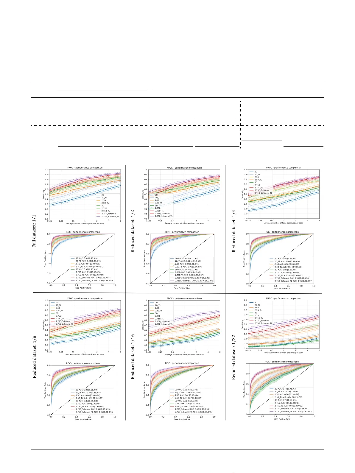
Loading high-quality paper...
Comments & Academic Discussion
Loading comments...
Leave a Comment